Classical Dynamics of Harmonically Trapped Interacting Particles

Abstract

Motivated by current interest in the dynamics of trapped quantum gases, we study the microcanonical dynamics of a trapped one-dimensional gas of classical particles interacting via a finite-range repulsive force of tunable strength. We examine two questions which have been of interest in quantum dynamics: (1) the breathing mode (size oscillation) dynamics of the trapped gas and the dependence of the breathing frequency on the interaction strength, and (2) the long-time relaxation and possible thermalization of the finite isolated gas. We show that the breathing mode frequency has non-monotonic dependence on the magnitude of the mutual repulsion, decreasing for small interactions and increasing for larger interactions. We explain these dependences in terms of slowing-down or speeding-up effects of two-body collision processes. We find that the gas thermalizes within a reasonable finite timescale in the sense of single-particle energies acquiring a Boltzmann distribution, only when the interaction strength is large compared to the energy per particle.

I Introduction

The non-equilibrium dynamics of isolated systems has been the subject of a large volume of work in recent years. In particular, in the quantum context, the study of unitary quantum evolution of many-body and few-body systems has undergone an explosive growth. This interest was partly fueled by the availability of experimental systems, e.g., trapped ultracold atomic and ionic systems, where non-dissipative dynamics can be studied explicitly due to excellent isolation from the environment. There are also foundational reasons for studying quantum dynamics in isolation: recent activity has led to advances in the understanding of basic principles connecting quantum dynamics, quantum chaos and the emergence of statistical mechanics and thermalization PolkovnikovRigol_AdvPhys2016 ; BorgonoviIzrailevSantos_PhysRep2016 . For classical many-body systems, explorations of the connections between microscopic dynamical rules, chaos, ergodicity and statistical mechanics have a much longer history, dating back to the time of Boltzmann and Poincaré Gaspard_book_1998 ; Dorfman_book_1999 ; Dumas_book_KAMstory ; Boltzmann_legacy_book ; EckmannRuelle_RMP85 ; Gaspard_PhysicaA06 .

Motivated by questions and issues arising in the field of quantum many-body and few-body dynamics, in this work we will study the classical dynamics of a collection of interacting particles confined in a one-dimensional harmonic trap. The analogs of two questions, studied intensively in the quantum literature, will be investigated for this classical system: (1) the influence of interactions on the breathing mode frequency of the trapped gas, and (2) the relaxation and possible thermalization of the finite system under its own evolution, in the absence of any external baths or dissipation mechanisms.

Experiments with cold atoms, which have an essential motivational role for the current interest in many-body quantum dynamics, are generally performed in a trapping potential, either optical or magnetic. As a result, in the last two decades many questions of many-body quantum physics have been reformulated in the presence of a harmonic trap. The presence of a harmonic trap often results in new dynamical phenomena. For example, the motion of vortices in a trapped condensate vortices_trappedBEC has new features, such as precession, compared to vortex motion in uniform condensates vortices_uniformBEC . Trapping also results in new collective phenomena which have no analog in uniform situations: for example, collective modes like dipole, breathing and quadrupole modes are specific to trapped many-body systems. Dipole modes (center of mass oscillations) and breathing modes (size oscillations) appear even for one-dimensional trapped systems; higher-dimensional systems display additional, more complicated modes like quadrupole and scissors modes. Because of the omnipresence of trapping potentials in cold-atom experiments, dipole and breathing mode dynamics are pervasive across the field: These modes have been intensively studied and used for diagnostic purposes since the early days of research with trapped quantum-degenerate gases, and continue to generate interest today collective_modes_early_papers ; PitaevskiiRosch_PRA97 ; Esslinger_exp_PRL2003 ; STG_Astrakharchik_PRL2005 ; GrimmSmith_unitaryfermions_PRA08 ; OrignacCitro_PRA08 ; Naegerl_Science09 ; Wetterich_JPB2011 ; Mazets_1Dbreathing_EPJD11 ; fermion2Dbreathing ; Tschischik_BHbreathing_PRA_2013 ; KroenkeSchmelcher_BM ; Bouchoule_PRL2014 ; br_mode_long_range_interactions ; Bonitz_Review ; QuinnHaque_PRA14 ; Tschischik_BH_2papers ; 1D_breathing_mode_recent ; Minguzzi_dipole_PRA2015 ; Stringari_lowDcollective_PRA15 ; MistakidisSchmelcher_PRA17 . In one of the best-known experiments on quantum many-body dynamics, Ref. NewtonsCradle_Nature06 , the dynamics of an integrable system (Lieb-Liniger bosons) was seen to have ultraslow relaxation in a trap, supposedly due to integrability. This experiment has led to continuing efforts to understand how a trap breaks integrability CauxKonik_glimmers_PRX15 ; CauxDoyonDubailKonik_1711 ; DoyonSpohn_JSTAT17 ; Moore_arXiv17.10 .

The presence of harmonic trapping is thus a paradigmatic aspect in the field of quantum non-equilibrium physics. This motivates our study of classical dynamics of trapped interacting particles. Similarly motivated by quantum dynamics, classical trapped dynamics of hard rods has recently been studied in Refs. DoyonSpohn_JSTAT17 ; Moore_arXiv17.10 , focusing on integrability-breaking effects of the trap. In this work, we consider trapped classical particles which interact via a simple finite-range potential between any pair of particles: a constant repulsive force acts whenever the particles are less than a certain distance apart. The interaction strength can be tuned, leading to different regimes of behavior.

Our first theme will be the breathing mode of the classical interacting gas, and the effect of interactions on the frequency of the breathing mode. In the quantum case, this has long been a topic of interest for both bosons and fermions. For bosons with short-range (contact) interactions, the situation has been studied in one, two and three dimensions. At zero interaction, the breathing mode is twice the trapping frequency $\omega_{0}$ in each case, assuming isotropic trapping. A mean field (Gross-Pitaevskii) calculation gives the frequency to be $\sqrt{D+2}$ times the trapping frequency, where $D$ is the spatial dimension. For three-dimensional (3D) traps, the mean-field description is expected to be qualitatively correct, thus the breathing mode frequency is expected to change monotonically from $2\omega_{0}$ at zero interactions to $\sqrt{5}\omega_{0}$ at large interactions. Remarkably, for 2D traps, the breathing frequency is exactly $2\omega_{0}$ for any interaction strength PitaevskiiRosch_PRA97 , due to a symmetry. Classical trapped particles with scale-invariant interaction potentials also have breathing frequency $2\omega_{0}$ independent of interaction strength PitaevskiiRosch_PRA97 . The interaction dependence in 1D (trapped Lieb-Liniger gas) is also remarkable: as the interaction is increased, the breathing frequency first decreases from $2\omega_{0}$ to the mean-field prediction $\sqrt{3}\omega_{0}$, and then at larger interactions increases again, returning to $2\omega_{0}$ in the infinite interaction (Tonks-Girardeau) limit Naegerl_Science09 ; Tschischik_BHbreathing_PRA_2013 ; 1D_breathing_mode_recent ; Bouchoule_PRL2014 ; KroenkeSchmelcher_BM . The breathing mode has also been investigated extensively for fermionic systems with contact interactions GrimmSmith_unitaryfermions_PRA08 ; fermion2Dbreathing ; Stringari_lowDcollective_PRA15 , and also for fermionic and bosonic systems with long-range interactions OrignacCitro_PRA08 ; br_mode_long_range_interactions ; Bonitz_Review . The breathing mode has also been studied for a high-temperature trapped gas where a Boltzmann-equation description is valid, both theoretically Guery-Odelin1999 and experimentally Cornell_classsical_3Dexpt_NatPhys15 .

In this work, we use an explicit microscopic model treated microcanonically, rather than a Boltzmann equation approach. Unlike the quantum case, the harmonic potential does not impose a length scale or an energy scale. The interaction range can thus be scaled away by a redefinition of length, i.e., by measuring lengths in units of the interaction range. There are thus only two important parameters determining the system behavior, namely the interaction strength and the energy per particle. We find that the breathing mode frequency has a non-monotonic dependence on the interaction parameter. At small interactions, when the particles pass through each other, the effect of collisions is to slow down the dynamics, so that the breathing frequency drops below the non-interacting value $2\omega_{0}$. At very large interactions, the particles bounce off each other, a process which speeds up the size oscillations, resulting in the breathing frequency being larger than $2\omega_{0}$.

Our second theme is the process of relaxation at longer timescales, and possible thermalization. This topic is also motivated by intense recent research in the quantum context. In quantum isolated systems, thermalization is now understood in terms of the so-called eigenstate thermalization hypothesis (ETH), which postulates that in ergodic systems the expectation values of observables in individual eigenstates depend ony on the eigenenergy, and hence represent the thermal value PolkovnikovRigol_AdvPhys2016 ; BorgonoviIzrailevSantos_PhysRep2016 ; ETH_Deutsch_Srednicki_Rigol . The connection to statistical mechanics is particularly difficult for explicitly finite systems, in which case ETH is to be understood in terms of finite size scaling Beugeling_ETHscaling_PRE14 . In classical systems, the connection between microscopic dynamics and statistical mechanics has been continually studied since the 19th century Gaspard_book_1998 ; Dorfman_book_1999 ; Dumas_book_KAMstory ; Boltzmann_legacy_book ; EckmannRuelle_RMP85 ; Gaspard_PhysicaA06 . It is generally understood that systems with nonzero Lyapunov exponents, i.e., chaotic or ergodic systems, thermalize in the long-time limit, provided there are enough degrees of freedom. As in the quantum case, finite systems are particularly intricate. In finite systems, defining thermalization is trickier as most observables will fluctuate or oscillate substantially. In addition, the influence of Kolmogorov-Arnold-Moser (KAM) orbits may play a role in preventing thermalization; it is generally believed that the fraction of phase space where KAM physics might be relevant decreases rapidly with particle number Dumas_book_KAMstory .

In our work, we examine the relaxation of our trapped interacting classical system, explicity for finite numbers of particles. We look for thermalization within finite timescales, by sampling single-particle energies periodically until such timescales and comparing the distribution of single-particle energies with the Boltzmann distribution. We show that whether or not the system thermalizes in this sense depends on the ratio of interaction strength and energy per particle. We also show that this result is reflected in the finite-time Lyapunov exponents of the system. We also examine another notion of thermalization, according to which a system is thermalized when it loses memory of initial state, by following the dynamics of the particle distribution in phase space. Remarkably, we find that one can observe energy thermaliztion even at timescales when the shape of the phase space distribution continues to perform seemingly coherent oscillations.

There is a significant literature on calculating Lyapunov exponents in model statistical-mechanics systems and thus exploring ergodicity Dorfman_book_1999 ; deWijn_fine ; Lyapunov_numerical_calculations ; Lyapunov_analytical_calculations ; FiniteTimeLyapunov . This provides intuition of what types of microscopic interactions are likely to produce thermalizability, and is an important step in the program of understanding statistical mechanics “from the bottom up”. However, we are not aware of a significant literature on following explicitly the microcanonical dynamics of statistical-mechanical or few-body systems. Several such studies have appeared recently DoyonSpohn_JSTAT17 ; Moore_arXiv17.10 ; JinKatsnelson_NJP13 , motivated by the quantum dynamics literature, like the present work. Another line of work has examined thermalization dynamics in one dimensional gravitational systems 1Dgravitational . Investigating such real-time dynamics can be expected to provide insights on the timescales and microscopic mechanisms involved in the emergence of statistical mechanics from collections of particles.

This paper is organized as follows: In Section II, we introduce the Hamiltonian, identify and introduce the essential scales, and describe some aspects of the model and our simulations. The breathing frequency is treated in Section III. We explain the main features using both real-space and phase space pictures of the interaction process, obtain estimates for the interaction- and energy-dependence of the frequency shift, and compare these predictions with numerics. Section IV treats relaxation and thermalization. We propose a condition for relaxation in reasonable timescales from considerations of few-body dynamics, compare the energy distribution with the Boltzmann distribution, show how the largest finite-time Lyapunov exponent distribution reflects the relaxation condition, and examine shape dynamics of the particle distribution in phase space. Concluding remarks appear in Section V.

II The model and its equilibrium properties

II.1 Model and Scaling

Our model for the interacting classical gas involves particles with a simple finite-range repulsive interaction. Two particles repel each other whenever they are within a distance $\sigma$ from each other. The force of repulsion is a constant, $F_{0}$, within this distance and zero when the distance is larger.

$$\Big{|}F(x)\Big{|}~{}=~{}\begin{cases}F_{0}&\quad|x|<\sigma\\ 0&\quad|x|>\sigma\end{cases}$$ (1)

where $|x|$ is the distance between two particles. This equation describes the magnitude of the interparticle force; the direction is always repulsive.

The gas contains $N$ such identical particles, each of mass $m$, in a harmonic trap. The Hamiltonian describing the gas is

$$H~{}=~{}\frac{1}{2}m\omega_{0}^{2}\sum_{i}x_{i}^{2}~{}+~{}\frac{1}{2}m\sum_{i}v_{i}^{2}~{}+~{}\sum_{\left|x_{i}-x_{j}\right|\textless\sigma}F_{0}\left(\sigma-\left|x_{i}-x_{j}\right|\right)$$ (2)

Here $F_{0}\left(\sigma-\left|r\right|\right)\theta(\sigma-|r|)$, with $r=x_{i}-x_{j}$ and $\theta()$ the Heaviside theta function, is the potential corresponding to the force introduced in Eq. (1). It is useful to rescale the quantities. We will measure distance, time, energy and force in units of $\sigma$, $1/\omega_{0}$, $m\omega_{0}^{2}\sigma^{2}$ and $m\omega_{0}^{2}\sigma$ respectively:

$$\tilde{x_{i}}=\frac{x_{i}}{\sigma}\ ,\quad\tilde{H}=\frac{H}{m\omega_{0}^{2}\sigma^{2}}\ ,\quad\tilde{t}=\omega_{0}t\ ,\quad\tilde{F_{0}}=\frac{F_{0}}{m\omega_{0}^{2}\sigma}\ .$$ (3)

Eq. 2 is then rewritten as

$$\tilde{H}=\frac{1}{2}\sum_{i}\tilde{x_{i}}^{2}+\frac{1}{2}\sum_{i}\left(\frac{d\tilde{x}_{i}}{d\tilde{t}}\right)^{2}+\sum_{\left|\tilde{x_{i}}-\tilde{x_{j}}\right|\textless 1}\tilde{F}_{0}\left(1-\left|\tilde{x_{i}}-\tilde{x_{j}}\right|\right)$$ (4)

Through this rescaling, we have reduced the number of the parameters in our model to three: the energy $\tilde{H}$, the interaction strength $\tilde{F_{0}}$, and the number of particles $N$. The rescaling is equivalent to setting $\sigma$, $\omega_{0}$ and $m$ to $1$; this is what we do in our numerical simulation. In the rest of this paper, we will use “$E$” and “$F_{0}$” to denote the reduced versions $\tilde{H}$ and $\tilde{F_{0}}$, and omit the tilde when writing rescaled quantities.

In the limit of infinite $F_{0}$, the particles maintain distance larger than $\sigma$ from each other. In this limit each particle can then be thought of as a ‘hard rod’ of length $2\sigma$. In the absence of a trap, this would be the one-dimensional classical system shown by Tonks to be classically integrable Tonks_1936 .

II.2 Cloud size or ‘radius’

We will be concerned with the size of the cloud. We quantify the size through the root-mean-square of particle positions $\left\{x_{i}\right\}$,

$$R~{}=~{}\left(\overline{x^{2}}\right)^{\frac{1}{2}}~{}=~{}\left(\frac{1}{N}\sum_{i}{x_{i}^{2}}\right)^{\frac{1}{2}}\,,$$ (5)

and refer to this quantity as the ‘radius’ or ‘cloud radius’. In the dilute gas limit, there are few or no interactions occuring at most times. Thus the energy $E$ is dominated by the trap energy, i.e., $E\approx m\omega_{0}^{2}\sum_{i}x_{i}^{2}=Nm\omega_{0}^{2}R^{2}$, or, in our units,

$$E~{}\approx~{}NR^{2}\,.$$ (6)

This approximation is good when the average distance betwen particles is much larger than the interaction range $\sigma=1$, i.e., whenever $R\gg 1$, which is the regime we consider dynamics in. Another way of describing this dilute-gas regime is that the gas is far from the ground state (described in the next subsection). Neglecting the interaction energy to estimate $E$ is reasonable even at very large interactions ($F_{0}\gg E/N$), because for very large interactions, the particles behave as hard rods which bounce off each other very rapidly, so that at most instants one can expect no collisions to be taking place, provided the gas is dilute. It is also expected to be a good approximation at very small $F_{0}$ since we can then simply neglect the interaction energy. Thus, we will use this as a common estimate for $R$ in terms of the energy.

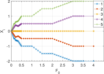
Figure 1: The ground state of a system with $N=5$ particles, shown via the positions of each particle, labeled 1 through 5. At large interactions, the particles position themselves just outside the range of interactions of the neighboring particles.

II.3 Ground states

The lowest-energy state of the system has zero kinetic energy; in this state the particles find stationary positions which minimize the trap (potential) and interaction energies. The trap potential tries to squeeze the particles towards the trap center, while the interaction tries to push them apart.

Because of the discontinuous ‘Heaviside theta’ form of our interaction, at large enough interactions (large $F_{0}$) the particles are spaced exactly at distance equal to the range $\sigma$, which is distance $1$ in our rescaled units. The interaction is then effectively a ‘hard-core’ interaction, or alternatively, the particles can be thought of as hard rods of length $2\sigma$.

At very small $F_{0}$, the particles in the ground state are close enough to the trap center that each particle interacts with every other particle. Equating the interaction force due to all the other particles with the trapping force, one finds that the position of the $i$-th particle is

$$x_{i}~{}=~{}\frac{2F_{0}}{m\omega_{0}^{2}}\left(i-\frac{N+1}{2}\right)~{}=~{}2F_{0}\left(i-\frac{N+1}{2}\right)$$ (7)

where the particles are labeled $i=1$ to $i=N$ from left to right. Thus the particles are equidistant in this regime. In this ‘solid’-like state, the low-lying excitation involves independent oscillation of the particles around their equilibrium position. In this regime, the distance between the leftmost and rightmost particles is at most $\sigma=1$. Thus, this situation extends up to $F_{0}=\frac{1}{2(N-1)}$. For the $N=5$ case shown in Figure 1, this behavior is seen up to $F_{0}<1/8$.

In Figure 1, we can see this crossover from the “solid-like” limit (left) to the “hardcore gas” limit (right). In between, there is a rich staircase-like structure, as the particles attempt to minimize the interaction by being at distance $>1$ from as many other particles as is compatible with the trap energy.

II.4 Phase space distribution

Figure 2: Upper (lower) panels are snapshots of the cloud configuration in phase space in the stationary (rotating) frame, at instants within the first trap period. Here $N=50$, $F_{0}=100$, and $E=50000$.

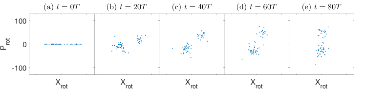
Figure 3: Phase space snapshots of the cloud dynamics viewed in the rotating frame, at longer timescales. The broadening and rotation observed here are interaction effects: in the non-interacting gas the particles are stationary in this frame.

A useful way to visualize the state and evolution of the gas is to plot the position and momentum of each particle, i.e., to plot the locations of the particles in the single-particle phase space. This will be useful for visualizing both the breathing mode and relaxation.

Figures 2 and 3 show such phase space snapshots. We generally start with particles distributed at random positions around the trap center, initially with no velocity (zero momentum). The initial state thus has the points lined up along the $X$ axis. In the absence of interactions, each particle would undergo simple harmonic oscillation with period $T=2\pi/\omega_{0}=2\pi$. The point corresponding to each particle executes clockwise elliptical motion around the $X$-$P$ plane. (In our units, the elliptical trajectory is actually circular.) This results in the distribution retaining its linear shape and rotating clockwise with exact period $T$. The effect of the interaction is to smear out the line and spread the points out toward a rotationally invariant distribution in the $X$-$P$ plane. The top panel of Figure 2 shows this during the first period and Figure 3 shows this process over a much longer timescale.

Since the rotation of the initial line of points is simple to understand as a single-particle (non-interacting) effect, we can focus on interaction effects by viewing the phase space in a ‘rotating’ frame. The rotating frame is used in the lower panel of Figure 2 and in Figure 3. In this picture, the ‘real’ $X$ and $P$ axes are rotating counter-clockwise. This rotating frame picture may be regarded as a classical version of the “interaction picture” of quantum dynamics. This picture highlights effects of interactions because the other effects are already encoded in the frame rotation.

In the absence of interactions, each point (each particle) is stationary in the rotating-frame phase space picture. As seen in the lower row of Figure 2 and in Figure 3, interactions cause a gradual distortion of the line as well as some degree of rotation. The rotation that is visible in the already rotating $X_{\rm rot}$-$P_{\rm rot}$ frame is the interaction-induced shift of the breathing frequency $\omega_{B}$ from the noninteracting value, $2\omega_{0}$. The distortion of the line toward an eventually rotationally invariant distribution may be regarded as thermalization or ergodicity. In the next sections we explore these two interaction-induced effects.

II.5 Numerical calculations

We use the Verlet algorithm (molecular dynamics) to numerically simulate the cloud, using particle numbers between 5 and 50. Our force is simple, so that calculating the force at each step is inexpensive, however, the theta function dependence of the force on particle positions requires the use of fine timesteps at the beginning and end of each collision process. The simulation is purely microcanonical: No external bath or thermalizing mechanisms are introduced.

The initial state is taken to have particles with zero velocity and random positions; hence the line distribution in the phase space picture. This has the advantage that the breathing motion is prominently visible. In addition, the question of long-time relaxation has the simple interpretation of evolving from the line distribution to a circularly symmetric distribution in phase space.

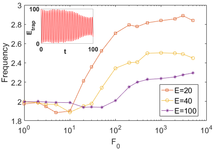
Figure 4: Breathing mode frequency measured at different $E$ and $F_{0}$, for $N=5$ particles. Inset: a demonstration of the oscillation of $E_{trap}$, the total potential energy of particles in the trap, Since $E_{trap}\propto\sum_{is}{x_{i}^{2}}$, it manifests the oscillation behavior of the radius $R(t)$ as defined in Eq. 5. The breathing frequency is obtained from the Fourier transform of $R(t)$.

III Breathing Frequency

We are interested in the oscillations of the size $R(t)$ of the cloud. It is convenient that our finite-size simulations start with a line distribution in phase space. If we started with a state whose configuration deviates only slightly from circular symmetry in $X$-$P$ space, the oscillating amplitude would be too small to be distinguished from noise.

Without interaction, the breathing mode frequency $\omega_{B}$ is exactly 2. This is visualized readily from the top panel of Figure 2, where $R(t)$ is the extent of the distribution in the horizontal ($X$) direction. As the line rotates clockwise with frequency $\omega_{0}=1$, within each period the line is twice horizontally aligned (maximum $R$) and twice vertically aligned (minimum $R$), so that the frequency of $R(t)$ is $\omega_{B}=2$. When there is interaction, the frequency will get shifted: $\omega_{B}=2+\delta$. Numerically, we measure the radius of the cloud $R(t)$ and get the frequency spectrum of its oscillation behavior by Fourier transform. Then we take the peak frequency near 2 as the breathing mode frequency.

III.1 Interaction-dependence

The frequency measured numerically for different $E$ and $F_{0}$ is shown in Figure 4 for a system with five particles, plotted as a function of $F_{0}$. The points each correspond to breathing-mode dynamics following from a single initial state; there is no averaging. The curves therefore show some noise. However, two prominent features are clear from these curves. At large interactions, $F_{0}\gg E$, the breathing frequency is larger than $2$, and saturates around a value which decreases with the system energy $E$. At small interactions, the breathing frequency is smaller than the non-interacting value $2$.

Below, we will provide a detailed phase space argument for these behaviors. However, a simple real-space picture explains both effects qualitatively as well. For very large $F_{0}$, when the interaction is ‘hard-core’-like, two particles exchange momentum instantaneously during a collision. By exchanging the labels of the particles during the collision, this can be interpreted as follows: particle $A$ carrying momentum $P_{A}$ jumps by distance $\sigma$ to the right, while particle $B$ carries its momentum $P_{B}$ and jumps by distance $\sigma$ to the left. In this manner, every collision will save a particle some time, $\frac{\sigma}{v}$. This translates into an increase of the breathing frequency. The speed $v$ per particle is on average $\sim\sqrt{E/N}$, and the number of collision each particle experiences in one period of harmonic oscillation is $\sim N$; hence we obtain $\delta\sim N^{\frac{3}{2}}E^{-\frac{1}{2}}$. When $F_{0}$ is smaller, we can no longer think of the particles as hard rods; the collisions now take finite time during which the speeds of the particles are slowed down and then sped up again, as they either cross paths or bounce from each other. When $F_{0}$ is small enough, this approaching time will at some critical value of $F_{0}$ consume the time saved by the finite range of the interaction. This explains why there is a small-$F_{0}$ regime for which the shift $\delta$ is negative. Figure 4 shows that this critical value of $F_{0}$, where $\delta$ changes sign and $\omega_{B}$ crosses $2$, increases with energy.

Figure 5: Schematic diagrams of two-particle collision process in the $X_{\rm rot}$-$P_{\rm rot}$ plane. The black filled dots shown locations of the two particles in $X_{\rm rot}$-$P_{\rm rot}$ space before the collision; the empty dots show locations after the collision. The dashed lines show the trajectories during the collision process. Collistions for different $F_{0}$ values are shown with different color. (a) When $F_{0}$ is large, particles cannot pass each other: during the collision the momentum changes sign. Being subject to a constant repulsive force, their trajectories during collision are curved arcs. The weaker $F_{0}$ is, the longer the collision lasts, and hence the more curved is the corresponding arc. For very strong interactions (red dashed line), particles exchange momenta instantaneously; hence the red dashed line is straight. The locations of the particles after this collision are on the gray line; the angle $\alpha$ made by this gray line is estimated in the text. The yellow, green, and blue dashed curves are for successively weaker interactions. (b) When $F_{0}$ is small, particles pass each other, so that the force they feel is discontinuous (changes sign) at the moment when they cross each other. Their trajectory in $X_{\rm rot}$-$P_{\rm rot}$ space has a corresponding turning point. The dashed bright blue trajectory is identical with the one in (a), which is the critical situation between passing and bouncing. In that case, particles have zero relative velocity when they collide.

III.2 Estimates using the rotating phase space

Since we are interested in the deviation $\delta=\omega_{B}-2$ from the non-interacting breathing frequency, it is useful to work in the rotating frame, in which a non-interacting cloud would be stationary (non-rotating). The rotation frequency of the cloud in this frame is then $\delta$.

To analyze the rotation relative to the $X_{\rm rot}$-$P_{\rm rot}$ frame, we consider two-particle collisions. In Figure 5(a), we show schematics of such collisions near the trap center at strong interactions. During the collision, the particle momentum is changing at a constant rate (the force is a constant repulsion), so the particle trajectory has a component of motion in the direction of the $P$ axis. However, the $P$ axis itself is rotating in the $X_{\rm rot}$-$P_{\rm rot}$ frame, at frequency $\omega_{0}$. Thus, the trajectories of the particles during the collision in the $X_{\rm rot}$-$P_{\rm rot}$ plane are curved arcs. As long as $F_{0}$ is large enough that the particles bounce off each other, the particle momentum will change sign, so a trajectory starting at negative $P$ will end at positive $P$. For very large $F_{0}$, the particles simply exchange momentum when they are at distance $\sigma$ from each other; this process is shown in red as two straight lines. (The particles are initially at $X=\pm\frac{1}{2}\sigma$ and remain at these $X$ values, but exchange their momenta.) For smaller $F_{0}$, there is change of both position and momentum, as shown in yellow, green and blue for successively weaker interactions.

The blue dashed line in Figure 5(a) shows a case where $F_{0}$ is small enough such that the particles can just cross each other. In Figure 5(b) we show collisions for even smaller $F_{0}$, so that the particles pass each other. The force changes direction discontinuously when the particles cross. In the $X_{\rm rot}$-$P_{\rm rot}$ plane, this is seen as a sharp turning point in the trajectory — if the momentum is initially positive, it first decreases and then increases again.

The boundary case between bouncing and passing behaviors is shown as the blue dashed curve in both 5(a) and 5(b). In this case, the momentum decreases to just about zero when the relative distance reaches zero, so that the particles just manage to cross.

We now estimate $\delta$ at large $F_{0}$. The relevant collision process is that shown by the red lines in Figure 5(a). The two particles, which are initially on the $X_{\rm rot}$ axis, are moved to two other points, on the thick gray line, which deviates a small angle $\alpha$ away from original configuration. In every period of the harmonic oscillation, each particle meets each of the other particles twice. Half of these collisions (about $N$ collisions) are between particles with large difference in momentum, which is the process shown in Fig.5. (As for the remaining half of the collisions, colliding particles have smaller difference in their momenta. In this estimate we ignore the effects of these collisions, as they clearly contribute far less to the rotation of the particle distribution.)

The precession angle is $\alpha\sim\sigma/P$, where $P$ is the momentum of the colliding particles. In our rescaled units, the typical momenta of interacting particles are of the order $R$. (In phase space $R$ can be interpreted either as the extent in real space when the velocities are small, or as the extent in momentum space when the particles approach $x=0$, i.e. when the distribution is along the $P$ direction.) Thus, we can estimate $\alpha\sim\sigma/R$, i.e., $\alpha\sim 1/R$, since our unit of length is $\sigma$. This is the rotation per unit collision. Since there are $\sim N$ collistions per period $T=2\pi$, we have the estimate for the interaction-induced rotation per unit time as

$$\delta~{}=~{}2\frac{N}{2\pi}\frac{1}{R}~{}=~{}\frac{1}{\pi}N^{3/2}E^{-1/2}$$ (8)

The factor $2$ accounts for the fact that each rotation of the elongated cloud in phase space corresponds to two breathing mode periods. In the last step we have used the estimate $E\sim NR^{2}$, Eq. (6).

The effect of interactions on the breathing frequency is more complicated at smaller $F_{0}$. As we have seen in Figure 4, a small $F_{0}$ can decrease the breathing frequency from its non-interacting value $\omega_{B}=2$. This can also be understood using phase space pictures of collision processes. For $F_{0}$ not very big, the finite interaction time needs to be taken into consideration. During this time, the point describing a particle in phase space moves along the direction of the $P$ axis at the rate $F_{0}/m$. Since the $P$ axis is itself rotating counter-clockwise in the $X_{\rm rot}$-$P_{\rm rot}$ frame, the particle will follow a curved trajectory in $X_{\rm rot}$-$P_{\rm rot}$ space, e.g., the yellow or green dashed lines in Fig. 5(a). The angle $\alpha$ that we used above to estimate $\delta$ thus decreases with the increase of interaction time; it is smaller for the yellow line and even opposite for the green line. This explains the negative contribution of interaction to $\delta$, for small enough values of $F_{0}$. At even smaller values of $F_{0}$, shown in Fig. 5)(b), the particles cross each other. The resulting final values are such that the line joining the post-interaction locations of the two particles has negative $\alpha$, i.e., is tilted clockwise with respect to the $X_{\rm rot}$ axis, meaning a negative contribution to the breathing frequency.

We can also estimate the critical value of $F_{0}$ for a given energy (or alternatively the critical value of $E$ for a given $F_{0}$) between positive and negative contributions to the breathing frequency. Since the $P$ axis rotates with frequency $\omega_{0}=1$ in the $X_{\rm rot}$-$P_{\rm rot}$ plane, the post-collision position of the particle in the $X_{\rm rot}$-$P_{\rm rot}$ plane makes angle $\omega_{0}\tau$ with the red line in Figure 5(a). Here $\tau$ is the time over which the interaction acts. The crossover between positive and negative $\delta$ is found by comparing this angle to $\alpha$:

$$\omega_{0}\tau=\alpha$$ (9)

The time $\tau$ is approximately the time it takes for the momentum to change sign due to a constant force $F_{0}$. Since the momentum is $\sim R$, this means $\tau\sim R/F_{0}$. Using our previous estimate $\alpha\sim\sigma/R$, together with $E\sim NR^{2}$, gives us the condition

$$\frac{E}{N}\sim F_{0}$$ (10)

for the breathing frequency to cross the non-interacting value $\omega_{B}=2$. This is roughly the same criterion for whether two particles will bounce or cross each other in a typical collision. (Note that this is only a rough correspondence: from the green arc in Figure 5(a), we see that the contribution to $\delta$ can be negative even when $F_{0}$ is strong enough for two particles to bounce off rather than pass each other.)

The condition (10) is consistent with Figure 4, where we noted that the critical $F_{0}$ grows with increasing energy.

III.3 Comparisons with numerical data

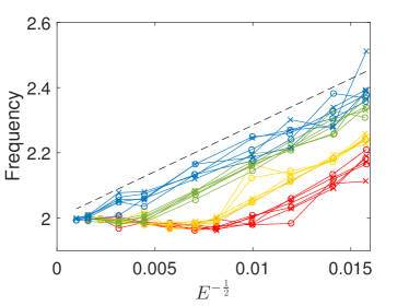
Figure 6: Dependence of breathing frequency, calculated for $N=20$ particles, on energy. Different colors represent different $F_{0}$ — red for $F_{0}=2\times 10^{3}$, yellow for $F_{0}=3\times 10^{3}$, green for $F_{0}=1\times 10^{4}$, and blue for $F_{0}=1\times 10^{5}$. Runs with three different initial states are shown in each case. In each run, the frequency is measured both in the time window 0-100 (labeled as crosses) and in the time window 900-1000 (labeled as circles). The black dashed line is the prediction of Eq. (8).

In Figure 6 we show a quantitative test of the main prediction, Eq. (8), of our analysis of the collision process. For large $F_{0}$, the frequency indeed scales as $E^{-1/2}$ and for $F_{0}=10^{5}$ is quite close to the actual numerical values prediction (8). Even for smaller $F_{0}$, at small enough energies (larger $E^{-1/2}$ values) the breathing mode becomes proportional to $E^{-1/2}$.

One might ask whether the breathing frequency predictions are also valid at late times, after the system has ‘relaxed’ from the initial line distribution in phase space to a more spread-out cloud, as we have seen in Figure 3. In Figure 6 we show the breathing frequency calculated from $R(t)$ oscillations in the first 100 time units, and also the frequency from data in a later time window. The frequencies appear to be overall stable and dependent primarily on $F_{0}$ and $E$.

IV Relaxation and Thermalization

For any nonzero interaction, the system is expected to be ergodic for $N>2$. Once there are many particles, one expects thermalization in the long-time limit. From the few-particle perspective, several interesting questions pose themselves. First, although we expect ergodicity, the question of how long it takes to thermalize is an open question for small $N$. We treat below a coarse-grained version of this question: namely, we ask whether particles show ergodic behavior within reasonable timescales chosen to be (somewhat arbitrarily) in the timestep range of $10^{3}$–$10^{4}$. Another question is the connection between energy thermalization as defined by the appearance of a Boltzmann distribution, and other intuitive characteristics of ergodic behavior such as whether the single-particle phase space is isotropically occupied. We find cases where one aspect is seen while the other is not.

IV.1 Few-particle considerations

Since we are interested in thermalization within finite timescales, it is useful to first consider mechanisms which hinder relaxation or thermalization. We begin with few-particle motion. Since ergodicity and relaxation are generally expected to be more robust and efficient with larger particle numbers, consideration of small particle numbers will highlight effects which slow down relaxation.

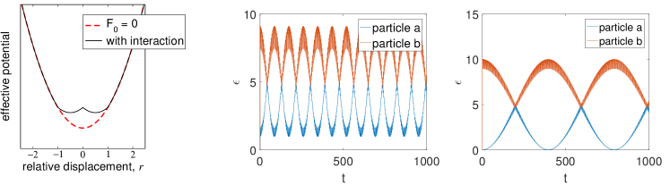
Figure 7: Two-particle dynamics. Left: Effective potential for relative motion. Center and right: evolution of the individual energies of the two particles. The two panels correspond to internal energy $E_{i}=2$ and $E_{i}=5$; the interaction is $F_{0}=1$. The beat frequency is lower for larger $E_{i}$.

IV.1.1 Two particles

We consider the two-particle motion in their center of mass frame. The center of mass itself executes simple harmonic oscillation. In the absence of interactions ($F_{0}=0$), the effective potential within the center of mass frame is itself parabolic, with the same frequency. So their relative motion is also a harmonic oscillation, with the same frequency $\omega_{0}$.

With interactions, a term $F_{0}(1-|r|)\theta(1-|r|)$ is added, where $r$ is the relative displacement; as shown in Figure 7. Now, the relative motion is no longer harmonic. When the internal energy is much larger than $F_{0}$, one could regard the resulting motion as having a slightly different frequency, or a collection of frequencies whose center is shifted slightly from $\omega_{0}$. Since the center-of-mass motion is still of frequency $\omega_{0}$, we have a superposition of slightly different frequencies, resulting in beating dynamics. This is clearly seen in the time evolution of individual energies shown in Figure 7. The two panels correspond to different internal energy $E_{i}$ (defined as the total energy minus the center-of-mass energy). For larger $E_{i}$, the distortion of the effective potential (at constant $F_{0}$) plays a smaller role in shifting the effective frequency of relative motion; hence the beat frequency is smaller.

This illustrates a simple mechanism hindering the redistribution of energy between particles, which is necessary for thermalization or relaxation. As seen in the example dynamics shown in Figure 7, the difference in energy between the two particles is sustained over time. Of course thermalization is not expected anyway in a two-particle system, but we will see below how this basic effect continues to play a role for larger $N$.

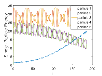
Figure 8: Time evolution of single-particle energies in a system of five particles, showing a case of inefficient energy redistribution. The energies of the two particles with highest energy (2 & 3) show a clear beating similar to the two-particle case, as does the pair 4 & 5, although less visible. The ‘unpaired’ particle 1 performs slow beating dynamics with the center of mass of the 4 & 5 pair — the energy of the particle 1 and of the center of mass of the 4 & 5 pair undergo long-period out-of-phase oscillations, of which approximately the first one-third of one period is visible in the time window shown.

IV.1.2 More particles

Once we have more than two particles, we expect chaotic or ergodic behavior. However, it is easy to imagine mechanisms which drastically slow down redistribution of energy.

Generally, whenever we have some particles with energy very different from others, the dynamics occurs mostly independently within groups of particles with similar energies. For example, with three particles, consider the situation where two of them, say A and B, have small internal energy, which means their mutual distance and relative velocity are both small, whereas the third particle (C) has some energy quite different from A and B. Then, A and B will often be interacting, and if their internal energy is smaller than $F_{0}$, significant energy exchange can occur between them. C will generally exchange little energy with the pair during interactions, in which (due to larger internal energy between C and either A or B), the interaction is not effective in energy exchange.

An example is shown in Figure 8, following the dynamics of $N=5$ particles. Two pairs of particles persist in performing ‘internal’ dynamics. The lone particle participates only in some slow beating motion with the center of mass of one of the pairs. Clearly, the energy mismatch acts as a hurdle to the relaxation process.

IV.2 Relaxation condition and the Boltzmann distribution

Our consideration of few-particle motion has shown that relaxation is slow when the internal energy of pairs is large compared to $F_{0}$. This allows us to conjecture a condition for relaxation in reasonable time. Although it is impossible to express the internal energy of every pair in terms of the total energy $E$, we can estimate the typical internal energy by the average energy, $E/N$. At least they are of the same order. Thus we have the condition

$$F_{0}\gtrsim\frac{E}{N}$$ (11)

for relaxation. This is the same condition we obtained in the previous section for the breathing frequency to be increased (rather than decreased) by the interaction.

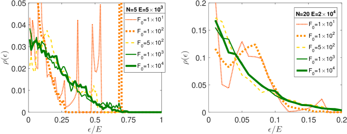
Figure 9: The distribution of single-particle energies. Snapshots of the single-particle energies are taken at unit time steps during the simulation, up to $\sim 10000$ time units. Green curves obey the relaxation condition (11), and yellow/orange corresponds to smaller $F_{0}$. The two panels correspond to different particle numbers $N$, but we choose total energies such that $E/N$ is identical ($=1000$) in all cases. Thus the threshold (11) corresponds to the interaction $F_{0}\sim 1000$.

Because the model is expected to be ergodic for $N>2$ particles, we expect the same condition to lead to thermalization. In fact, the proposed condition works even quantitatively, as we show in Figure 9. Here, the distribution of energies among the different particles is presented. Given our small particle number, a single snapshot of the energies will not yield enough statistics to investigate the distribution of single-particle energies. Therefore, single-particle energies are recorded once every time unit (i.e., at time intervals of $1/\omega_{0}$) as the simulation evolves, up to around $t\sim 10^{4}$. The distribution of these observed values then shows whether or not the system has thermalized to a Boltzmann distribution. In the two panels of Figure 9, we show the distributions obtained for a $N=5$ system and a $N=20$ system. In both cases, we choose the total energy to be $E=1000N$. In accordance with our conjectured condition, we find that the observed single-particle distributions are qualitatively different for $F_{0}\gtrsim 1000$ and for smaller interactions. When the “thermalization condition” $F_{0}\gtrsim E/N$ is satisfied, the distribution is roughly exponential ($\sim e^{-\beta\epsilon})$. For smaller $F_{0}$, thermalization in this sense is not seen in the single-particle energy distribution. Since the systems are expected to be ergodic, the smaller-$F_{0}$ systems presumably will also eventually show a Boltzmann distribution of energy, but only at (much) longer timescales.

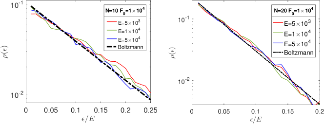
Figure 10: Complaring the single-particle energy distribution $\rho(\epsilon)$ with the Boltzmann distribution. The energy values all satisfy the relaxation condition (11). The Boltzmann distribution $\propto e^{-\beta\epsilon}$, with the temperature defined as $\beta^{-1}=E/N$, is the thick dashed line.

In Figure 10, we display the agreement with the Boltzmann distribution in several ‘thermalizing’ situations, $F_{0}\gtrsim E/N$. In each panel, the calculated distributions from simulations is plotted against the Boltzmann distribution. The overall agreement shows that the energy is well-thermalized among the particles on average within the timescales under consideration.

There are some small deviations from the Boltzmann distribution visible in Figure 10. Most of the deviation is probably due to numerical noise, and unsurprising given our small system sizes. However, some deviation is also expected due to the contribution of the density of states (DOS), as the probability of finding an energy is proportional to the Boltzmann exponential factor multiplied by the DOS. For the simple harmonic oscillator, the DOS is constant. The interaction deforms the energy shell in the small region $|x_{i}-x_{j}|<\sigma$; so that the DOS is no longer a constant. The measured distribution seems systematically slightly smaller than the Boltzmann curve at very small $\epsilon$. For larger interactions, small energies are expected to be penalized, as the interaction opposes particles clustering at small velocities near the bottom of the trap. This may be the reason for the counts in Fig.10 being slightly lower than the Boltzmann prediction at small $\epsilon$. However, since we are in the regime of a dilute gas ($\sigma\ll R$), the effect is quite small.

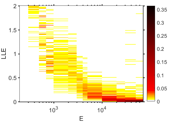
Figure 11: The distribution of largest Lyapunov exponents, for $N=5$, $F_{0}=1000$, at different energies. The color indicates the observed probability of a measured LLE value being found in a bin; the bins are of size 0.01. The average of the distribution decreases monotonically with energy.

IV.3 Lyapunov Exponents

The general idea that thermalization is faster for larger $F_{0}/E$ can be quantified through the Lyapunov exponents. For high-dimensional systems, there is a spectrum of exponents which manifests the instability of the trajectory along each direction. The largest Lyapunov exponent (LLE) reflects the shortest time scale for the system to lose memory of the initial state. To calculate the LLE, we follow the method described, e.g., in Ref. EckmannRuelle_RMP85 . If the calculation is carried out up to sufficiently late times, the LLE for an ergodic system is uniquely defined and independent of the starting state. We would like to deal with parameter regimes both within and outside our relaxation condition, $E<F_{0}N$ and $E>F_{0}N$, and in the latter case we have seen that ergodicity does not become apparent at reasonable timescales. Therefore, we carry out the computation of the LLE up to $t\sim 10^{3}$, i.e, we consider finite-time Lyapunov exponents FiniteTimeLyapunov . The LLE estimates obtained in this way depend on the initial configuration. The collection of these estimates forms a distribution. We show the distributions in Figure 11 for fixed $F_{0}$ and different values of the total energy $E$. The distributions are obtained using 100 initial states in each case.

The average LLE decreases with the increase of energy. The critical part is near $E=F_{0}N=5000$. Around this value, the most probable value of LLE decreases well below $\sim 1$, which indicates that the shortest time scale becomes much longer than an oscillation period when $E\gtrsim 5000$. This is consistent with our predicted thermalization threshold. As $E$ increases far beyond the thermalization threshold value, the LLE distribution is close to zero, suggesting a divergence of relaxation time. We have thus shown an explicit correspondence between energy thermalization in real time and the (finite-time) LLE.

For the largest $E$ values (smallest $F_{0}/E$) in Figure 11, we note large relative fluctuations. This presumably reflects the fact that the relaxation time in these cases is much larger than the time used to calculate the finite-time LLE’s.

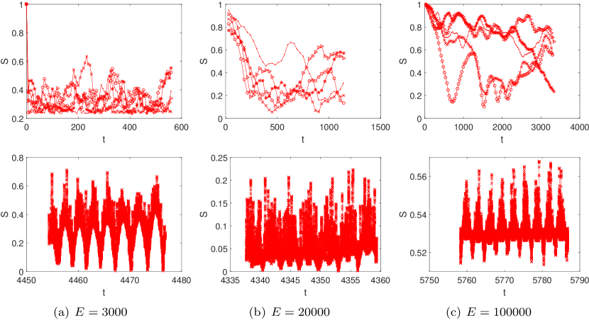
Figure 12: $N=20,F_{0}=1000$. Time evolution of the shape parameter, $S(t)$, for $N=20$ particles, $F_{0}=1000$. The three columns correspond to $E<F_{0}N$ (low-energy or thermalizing regime), $E=F_{0}N$ (intermediate regime), and $E>F_{0}N$ (high-energy or non-thermalizing regime). In the top row, coarse-grained values (averaged over 10 periods) are shown, for several initial states with the same energy in each case. The lower row shows original data (not averaged) in a window after several thousand time steps.

IV.4 Shape of distribution in single-particle phase space

Until now, we have formulated the thermalization question in terms of energy distributions. More generally, thermalization may be taken to mean that a many-body system loses memory of its initial state. In the single-particle phase space picture, Figures 2 and 3, our initial state is very special: The particles are lined up along the $X$ axis. The effect of interaction is to distort this line toward a circularly symmetric distribution. Thus, we would consider that the memory of the initial state is lost when the distribution of points in the $X$-$P$ plane are not elongated in any one direction.

To quantify the shape of distribution in phase space, we define a shape parameter $S$ measuring the degree of ellipticity:

$$S=\frac{a-b}{a+b}$$ (12)

where $a$ and $b$ are the long axis and the short axis of the inertia ellipse in phase space respectively. These are calculated by diagonalizing the inertia tensor I: $I_{xx}=\sum{p^{2}},I_{xp}=I_{px}=-\sum{xp},I_{pp}=\sum{x^{2}}$. The shape parameter is $S=1$ for line-shaped distributions and $S=0$ for circularly symmertic distributions.

In a thermalizing system with very large $N$, one might expect that $S(t)$ will decrease rapidly to zero, and a reasonable conjecture is that the timescale for the decrease (relaxation) of $S(t)$ should be related to the timescale for achieving energy thermalization. However, in our finite systems, we will find that $S(t)$ can continue to perform coherent oscillations long after single-particle thermalization has been observed.

The time evolution of the shape parameter $S$ is shown in Fig.12. The top three panels show averaged values of $S$ in order to highlight the overall behavior. Every data point is the average of the original data over $10T=20\pi$. (The dynamics for several initial states are shown to give an impression of typical $S(t)$ dynamics.) The bottom-row panels show the original data measured in a time window starting after several thousand time units.

The coarse-grained (averaged) dynamics in the top row reflects our intuition that there is slower relaxation at larger $E/F_{0}$. We see a much faster decay for small $E/F_{0}$, i.e., in the thermalizing regime. The behavior of $S(t)$ at longer times shows (bottom row) that there are coherent oscillations of the phase space cloud shape on rather long timescales. Strikingly, this is even true for the thermalizing regime (bottom left panel), for which the time-averaged single-particle energies already are Boltzmann-distributed. Thus, energy thermalization can occur at timescales much faster than it takes for other features of the gas to relax.

V Discussion and Conclusions

Considering classical interacting particles in a harmonic trap, we have addressed two non-equilibirum problems motivated by analogous questions in recent research on quantum many-body dynamics. We have chosen to work with a simple finite-range interaction with variable interaction strength, in the ‘dilute gas’ regime where the particles are at an average distance significantly larger than the interaction range.

The first question concerned the breathing mode of the classical trapped gas, and the influence of interaction on the breathing mode frequency. We have shown nontrivial dependence of the breathing frequency on the interaction strength $F_{0}$: the breathing frequency first decreases as a function of $F_{0}$, and around the critical value $F_{0}\sim E/N$, increases above the non-interacting value. Eventually at large $F_{0}$ the frequency shift reaches a plateau at a value $\propto\sqrt{N^{3}/E}$. We have explained this behavior physically, using both real-space and phase space pictures.

The second question concerned the relaxation and thermalization behavior of the gas. This is particularly interesting for a moderate number of particles, far from the thermodynamic limit. We have examined thermalization in the sense of single-particle energy distribution; this has to be carefully defined when the number of particles is in the ‘mesoscopic’ regime. Sampling the single-particle energies from temporal snapshots of the system over a period of time, we find that the system ‘thermalizes’ in reasonable time for $F_{0}\gtrsim E/N$. We have explained this condition in terms of relaxation-hindering mechanisms for few-particle systems. We have also shown that this threshold corresponds to the largest finite-time Lyapunov exponent exceeding $\approx 1$. Finally, we have found that (for $F_{0}>E/N$) thermalization occurs at timescales much faster than the timescale for the breathing mode oscillations to damp out. This is remarkable if one expects thermalization to correspond to the loss of memory of initial conditions: the initial shape ellipticity of the phase space cloud provides very-long-lived oscillations of the shape of the phase space distribution, even after energy thermalization has already occurred. Of course, it is known quite generally that different observables can have different equilibration times.

The present work opens up various questions. Our chosen form of interaction is simple and sensible as a model interaction; and we expect that the $F_{0}$-dependence of the breathing mode frequency represents the interaction-dependence for a wide class of interactions. However, it would be interesting to ask how collective modes in general depend on the form of interactions. For example, if the force were partially or totally attractive, e.g., if $F_{0}$ is negative, or with a Lennard-Jones type potential which is attractive for some separations, the effect on the breathing frequency is not obvious. While the connection between ergodicity and thermalization is expected to be simpler in large systems, for few-body systems like the present case the connection is less clear and raises questions of the parametric dependence of timescales on model parameters. Our study of a special case exemplifies the need for better general understanding of the connections between relaxation timescales, interaction strengths, thermalization, and finite-time Lyapunov exponents.

References

- (1) L. D’Alessio, Y. Kafri, A. Polkovnikov, and M. Rigol, “From quantum chaos and eigenstate thermalization to statistical mechanics and thermodynamics”, Adv. Phys., 65, 239 (2016).
- (2) F. Borgonovi, F. M. Izrailev, L. F. Santos, and V. G. Zelevinsky, “Quantum chaos and thermalization in isolated systems of interacting particles”, Phys. Rep. 626, 1 (2016).
- (3) P. Gaspard, “Chaos, Scattering, and Statistical Mechanics”, Cambridge University Press, 1998.
- (4) J. P. Dorfman, “An Introduction to Chaos in Non-equilibrium Statistical Mechanics”, Cambridge University Press, 1999.
- (5) H. S. Dumas: “The KAM Story: A Friendly Introduction to the Content, History, and Significance of Classical Kolmogorov-Arnold-Moser Theory”, World Scientific, 2014.
- (6) “Boltzmann’s Legacy”, edited by G. Gallavotti, W. L. Reiter, and J. Yngvason; European Mathematical Society, 2007.
- (7) J.-P. Eckmann and D. Ruelle, “Ergodic theory of chaos and strange attractors”, Rev. Mod. Phys., 57, 617 (1985).
- (8) P. Gaspard, “Hamiltonian dynamics, nanosystems, and nonequilibrium statistical mechanics”, Physica A, 369, 201 (2006).
-
(9)
D. S. Rokhsar,
“Vortex Stability and Persistent Currents in Trapped Bose Gases”,
Phys. Rev. Lett., 79, 2164 (1997).
A. A. Svidzinsky and A. L. Fetter, “Stability of a Vortex in a Trapped Bose-Einstein Condensate”, Phys. Rev. Lett., 84, 5919 (2000).
B. P. Anderson, P. C. Haljan, C. E. Wieman, and E. A. Cornell, “Vortex Precession in Bose-Einstein Condensates: Observations with Filled and Empty Cores”, Phys. Rev. Lett. 85, 2857 (2000).
A. L. Fetter and A. A. Svidzinsky, “Vortices in a trapped dilute Bose-Einstein condensate”, J. Phys.: Condens. Matter, 13, R135 (2001).
W. Li, M. Haque, and S. Komineas, “Vortex dipole in a trapped two-dimensional Bose-Einstein condensate”, Phys. Rev. A, 77, 053610 (2008).
A. L. Fetter, “Rotating trapped Bose-Einstein condensates”, Rev. Mod. Phys., 81, 647 (2009).
D. V. Freilich, D. M. Bianchi, A. M. Kaufman, T. K. Langin, and D. S. Hall, “Real-Time Dynamics of Single Vortex Lines and Vortex Dipoles in a Bose-Einstein Condensate”, Science, 329, 1182 (2010).
T. W. Neely, E. C. Samson, A. S. Bradley, M. J. Davis, and B. P. Anderson “Observation of Vortex Dipoles in an Oblate Bose-Einstein Condensate”, Phys. Rev. Lett., 104, 160401 (2010).
R. Navarro, R. Carretero-González, P. J. Torres, P. G. Kevrekidis, D. J. Frantzeskakis, M. W. Ray, E. Altuntaş, and D. S. Hall, “Dynamics of a Few Corotating Vortices in Bose-Einstein Condensates”, Phys. Rev. Lett., 110, 225301 (2013). -
(10)
A. L. Fetter,
“Vortices in an Imperfect Bose Gas. I. The Condensate”,
Phys. Rev., 138, A429 (1965).
A. L. Fetter, “Vortices in an Imperfect Bose Gas. IV. Translational Velocity”, Phys. Rev., 151, 100 (1966).
R. J. Donnelly, “Quantized vortices in Helium II”, Cambridge University Press, 1991. -
(11)
S. Stringari, “Collective Excitations of a Trapped
Bose-Condensed Gas”, Phys. Rev. Lett. 77, 2360 (1996).
M.-O. Mewes, M. R. Andrews, N. J. van Druten, D. M. Kurn, D. S. Durfee, C. G. Townsend, and W. Ketterle, “Collective Excitations of a Bose-Einstein Condensate in a Magnetic Trap”, Phys. Rev. Lett., 77, 988 (1996).
D. S. Jin, J. R. Ensher, M. R. Matthews, C. E. Wieman, and E. A. Cornell, “Collective excitations of a bose-einstein condensate in a dilute gas,” Phys. Rev. Lett., 77, 420 (1996).
F. Dalfovo, S. Giorgini, M. Guilleumas, L. Pitaevskii, and S. Stringari, “Collective and single-particle excitations of a trapped bose gas,” Phys. Rev. A, 56, 3840 (1997).
M. Amoruso, I. Meccoli, A. Minguzzi, and M. P. Tosi, “Density profiles and collective excitations of a trapped two component Fermi vapour”, Eur. Phys. J. D 8, 361 (2000).
R. Combescot and X. Leyronas, “Hydrodynamic Modes in Dense Trapped Ultracold Gases”, Phys. Rev. Lett., 89, 190405 (2002).
F. Chevy, V. Bretin, P. Rosenbusch, K. W. Madison, and J. Dalibard, “Transverse Breathing Mode of an Elongated Bose-Einstein Condensate”, Phys. Rev. Lett., 88, 250402 (2002).
C. Menotti and S. Stringari, “Collective oscillations of a one-dimensional trapped Bose-Einstein gas”, Phys. Rev. A 66, 043610 (2002).
J. Fuchs, X. Leyronas, and R. Combescot, “Hydrodynamic modes of a one-dimensional trapped Bose gas”, Phys. Rev. A, 68, 043610 (2003). - (12) L. P. Pitaevskii and A. Rosch, “Breathing modes and hidden symmetry of trapped atoms in two dimensions”, Phys. Rev. A 55, R853 (1997);
- (13) H. Moritz, T. Stöferle, M. Köhl, and T. Esslinger, “Transition from a Strongly Interacting 1D Superfluid to a Mott Insulator”, Phys. Rev. Lett., 91, 250402 (2003).
- (14) G. E. Astrakharchik, J. Boronat, J. Casulleras, and S. Giorgini, “Beyond the Tonks-Girardeau Gas: Strongly Correlated Regime in Quasi-One-Dimensional Bose Gases”, Phys. Rev. Lett., 95, 190407 (2005).
- (15) S. Riedl, E. R. Sánchez Guajardo, C. Kohstall, A. Altmeyer, M. J. Wright, J. Hecker Denschlag, R. Grimm, G. M. Bruun, and H. Smith, “Collective oscillations of a Fermi gas in the unitarity limit: Temperature effects and the role of pair correlations”, Phys. Rev. A 78, 053609 (2008).
- (16) Pedri, S. De Palo, E. Orignac, R. Citro, and M. L. Chiofalo, “Collective excitations of trapped one-dimensional dipolar quantum gases”, Phys. Rev. A, 77, 015601 (2008).
- (17) E. Haller, M. Gustavsson, M. J. Mark, J. G. Danzl, R. Hart, G. Pupillo, H.-C. Nägerl, “Realization of an excited, strongly correlated quantum gas phase,” Science, 325, 1224 (2009).
- (18) I. Boettcher, S. Floerchinger, and C. Wetterich, “Hydrodynamic collective modes for cold trapped gases”, J. Phys. B, 44, 235301 (2011).
- (19) I. E. Mazets, “Integrability breakdown in longitudinaly trapped, one-dimensional bosonic gases”, Eur. Phys. J. D 65, 43 (2011).
-
(20)
E. Vogt, M. Feld, B. Fröhlich, D. Pertot, M. Koschorreck, and M. Köhl, “Scale Invariance and
Viscosity of a Two-Dimensional Fermi Gas”, Phys. Rev. Lett. 108, 070404 (2012).
Chao Gao and Zhenhua Yu, “Breathing mode of two-dimensional atomic Fermi gases in harmonic traps”, Phys. Rev. A 86, 043609 (2012).
J. Hofmann, “Quantum Anomaly, Universal Relations, and Breathing Mode of a Two-Dimensional Fermi Gas”, Phys. Rev. Lett. 108, 185303 (2012).
S. K. Baur, E. Vogt, M. Köhl, and G. M. Bruun, “Collective modes of a two-dimensional spin-1/2 Fermi gas in a harmonic trap”, Phys. Rev. A 87, 043612 (2013).
B. P. van Zyl, E. Zaremba, and J. Towers, “Collective excitations of a harmonically trapped, two-dimensional, spin-polarized dipolar Fermi gas in the hydrodynamic regime”, Phys. Rev. A 90, 043621 (2014).
Y.-C. Zhang and S.Zhang, “Strongly interacting p -wave Fermi gas in two dimensions: Universal relations and breathing mode”, Phys. Rev. A 95, 023603 (2017). - (21) W. Tschischik, R. Moessner, M. Haque, “Breathing mode in the Bose-Hubbard chain with a harmonic trapping potential”, Phys. Rev. A, 88, 063636 (2013).
- (22) R. Schmitz, S. Krönke, L. Cao, and P. Schmelcher, “Quantum breathing dynamics of ultracold bosons in one-dimensional harmonic traps: Unraveling the pathway from few- to many-body systems”, Phys. Rev. A, 88, 043601 (2013).
- (23) B. Fang, G. Carleo, A. Johnson, and I. Bouchoule, “Quench-Induced Breathing Mode of One-Dimensional Bose Gases”, Phys. Rev. Lett. 113, 035301 (2014).
-
(24)
S. Bauch, K. Balzer, C. Henning, and M. Bonitz,
“Quantum breathing mode of trapped bosons and fermions at arbitrary coupling”,
Phys. Rev. B, 80, 054515 (2009).
J. W. Abraham, K. Balzer, D. Hochstuhl, and M. Bonitz, “Quantum breathing mode of interacting particles in a one-dimensional harmonic trap”, Phys. Rev. B, 86, 125112 (2012).
C. R. McDonald, G. Orlando, J. W. Abraham, D. Hochstuhl, M. Bonitz, and T. Brabec, “Theory of the Quantum Breathing Mode in Harmonic Traps and its Use as a Diagnostic Tool”, Phys. Rev. Lett., 111, 256801 (2013).
J. W. Abraham, M. Bonitz, C. McDonald, G. Orlando, and T. Brabec, “Quantum breathing mode of trapped systems in one and two dimensions”, New J. Phys, 16, 013001 (2014). - (25) J. W. Abraham, and M. Bonitz, “Quantum Breathing Mode of Trapped Particles: from nanoplasmas to ultracold gases”, Contrib. Plasma Physics, 54, 27 (2014).
- (26) E. Quinn and M. Haque, “Modulated trapping of interacting bosons in one dimension”, Phys. Rev. A, 90, 053609 (2014).
-
(27)
W. Tschischik and M. Haque, “Repulsive-to-attractive interaction
quenches of a one-dimensional Bose gas in a harmonic trap”, Phys. Rev. A, 91,
053607 (2015).
W. Tschischik, R. Moessner, and M. Haque, “Bose-Hubbard ladder subject to effective magnetic field: Quench dynamics in a harmonic trap”, Phys. Rev. A, 92, 023845 (2015). - (28) G. De Rosi and S. Stringari, “Collective oscillations of a trapped quantum gas in low dimensions”, Phys. Rev. A 92, 053617 (2015).
- (29) M. Cominotti, F. Hekking, and A. Minguzzi, “Dipole mode of a strongly correlated one-dimensional Bose gas in a split trap: Parity effect and barrier renormalization”, Phys. Rev. A, 92, 033628 (2015).
-
(30)
A. Iu. Gudyma, G. E. Astrakharchik, and M. B. Zvonarev, “Reentrant behavior of the
breathing-mode-oscillation frequency in a one-dimensional Bose gas”,
Phys. Rev. A, 92, 021601(R) (2015).
S. Choi, V. Dunjko, Z. D. Zhang, and M. Olshanii, “Monopole Excitations of a Harmonically Trapped One-Dimensional Bose Gas from the Ideal Gas to the Tonks-Girardeau Regime”, Phys. Rev. Lett. 115, 115302 (2015)
X.-L. Chen, Y. Li, and H. Hu, “Collective modes of a harmonically trapped one-dimensional Bose gas: The effects of finite particle number and nonzero temperature”, Phys. Rev. A 91, 063631 (2015). - (31) S. I. Mistakidis and P. Schmelcher, “Mode coupling of interaction quenched ultracold few-boson ensembles in periodically driven lattices”, Phys. Rev. A, 95, 013625 (2017).
- (32) T. Kinoshita, T. Wenger, and D. S. Weiss, “A quantum Newton’s cradle”, Nature, 440, 900 (2006).
- (33) G. P. Brandino, J.-S. Caux, R. M. Konik, “Glimmers of a Quantum KAM Theorem: Insights from Quantum Quenches in One Dimensional Bose Gases”, Phys. Rev. X, 5, 041043 (2015).
- (34) J.-S. Caux, B. Doyon, J. Dubail, R. Konik, and T. Yoshimura, “Hydrodynamics of the interacting Bose gas in the Quantum Newton Cradle setup”, arXiv:1711.00873.
- (35) B. Doyon and H. Spohn, “Dynamics of hard rods with initial domain wall state”, J. Stat. Mech., 2017, 073210 (2017).
- (36) X. Cao, V. B. Bulchandani, J. E. Moore, “Incomplete thermalization from trap-induced integrability breaking: lessons from classical hard rods”, arXiv:1710.09330.
- (37) D. Guéry-Odelin, F. Zambelli, J. Dalibard, and S. Stringari, “Collective oscillations of a classical gas confined in harmonic traps,” Phys. Rev. A, 60, 4851 (1999).
- (38) D. S. Lobser, A. E. S. Barentine, E. A. Cornell, and H. J. Lewandowski, “Observation of a persistent non-equilibrium state in cold atoms”, Nat Phys 11, 1009 (2015).
-
(39)
J. M. Deutsch, “Quantum statistical mechanics in a closed system”, Phys. Rev. A, 43, 2046 (1991).
M. Srednicki, “Chaos and quantum thermalization”, Phys. Rev. E, 50, 888 (1994).
M. Rigol, V. Dunjko, and M. Olshanii, “Thermalization and its mechanism for generic isolated quantum systems”, Nature, 452, 854 (2008). - (40) W. Beugeling, R. Moessner, and M. Haque, “Finite-size scaling of eigenstate thermalization”, Phys. Rev. E, 89, 042112 (2014).
-
(41)
A. S. de Wijn, B. Hess, and B. V. Fine,
“Largest Lyapunov Exponents for Lattices of Interacting Classical Spins”,
Phys. Rev. Lett. 109, 034101 (2012).
A. S. de Wijn, B. Hess, and B. V. Fine, “Chaotic properties of spin lattices near second-order phase transitions”, Phys. Rev. E, 92, 062929 (2015).
A. S. de Wijn, B. Hess, and B. V. Fine, “Lyapunov instabilities in lattices of interacting classical spins at infinite temperature”, J. Phys. A: Math. Theor., 46, 254012 (2013). -
(42)
C. Dellago and H. A. Posch,
“Kolmogorov-Sinai entropy and Lyapunov spectra of a hard-sphere gas”
Physica A, 240, 68 (1997).
V, Latora, A. Rapisarda, and S. Ruffo, “Lyapunov Instability and Finite Size Effects in a System with Long-Range Forces”, Phys. Rev. Lett., 80, 692 (1998).
W. G. Hoover, H. A. Posch, C. Forster, C. Dellago, and M. Zhou, “Lyapunov Modes of Two-Dimensional Many-Body Systems; Soft Disks, Hard Disks, and Rotors”, J. Stat. Phys. , 109, 765 (2002). -
(43)
D. M. Barnett, T. Tajima, K. Nishihara, Y. Ueshima, and H. Furukawa,
“Lyapunov Exponent of a Many Body System and Its Transport Coefficients”,
Phys. Rev. Lett., 76, 1812 (1996).
H. van Beijeren, J. R. Dorfman, H. A. Posch, and Ch. Dellago, “Kolmogorov-Sinai entropy for dilute gases in equilibrium”, Phys. Rev. E, 56, 5272 (1997).
R. van Zon, H. van Beijeren, and Ch. Dellago, “Largest Lyapunov Exponent for Many Particle Systems at Low Densities”, Phys. Rev. Lett., 80, 2035 (1998).
S. McNamara and M. Mareschal, “Origin of the hydrodynamic Lyapunov modes”, Phys. Rev. E, 64, 051103 (2001).
A. S. de Wijn and H. van Beijeren, “Goldstone modes in Lyapunov spectra of hard sphere systems”, Phys. Rev. E, 70, 016207 (2004).
A. S. de Wijn, “Lyapunov spectra of billiards with cylindrical scatterers: Comparison with many-particle systems”, Phys. Rev. E, 72, 026216 (2005). -
(44)
E. Ott, “Chaos in Dynamical Systems”, Cambridge University Press, 1993.
M. A. Sepúlveda, R Badii, and E. Pollak, “Spectral analysis of conservative dynamical systems”, Phys. Rev. Lett., 63, 1226 (1989).
C. Amitrano and R. S. Berry. “Probability distributions of local Lyapunov exponents for Hamiltonian systems”, Phys. Rev. E, 47, 3158 (1993).
F. K. Diakonos, D. Pingel, and P. Schmelcher “Analyzing Lyapunov spectra of chaotic dynamical systems”, Phys. Rev. E, 62, 4413 (2000).
H. Schomerus and M. Titov, “Statistics of finite-time Lyapunov exponents in a random time-dependent potential”, Phys. Rev. E, 66, 066207 (2002).
M. W. Beims, C. Manchein, and J. M. Rost, “Origin of chaos in soft interactions and signatures of nonergodicity”, Phys. Rev. E, 76, 056203 (2007).
C. Manchein, M. W. Beims, and J. M. Rost, “Characterizing the dynamics of higher dimensional nonintegrable conservative systems”, Chaos, 22, 033137 (2012).
S. Sawada and T. Taniguchi, “Chaos and ergodicity of two hard disks within a circular billiard”, Phys. Rev. E, 88, 022907 (2013).
K. Kanno and A. Uchida, “Finite-time Lyapunov exponents in time-delayed nonlinear dynamical systems”, Phys. Rev. E, 89, 032918 (2014).
D, Pazó, J. M. López, and A. Politi, “Diverging Fluctuations of the Lyapunov Exponents” Phys. Rev. Lett., 117, 034101 (2016). - (45) F. Jin, T. Neuhaus, K. Michielsen, S. Miyashita, M. A. Novotny, M. I. Katsnelson, and H. D. Raedt, “Equilibration and thermalization of classical systems,” New Journal of Physics, 15, 033009 (2013).
-
(46)
K. R. Yawn and B. N. Miller, “Ergodic properties and equilibrium of
one-dimensional self-gravitating systems,” Phys. Rev. E, 56, 2429 (1997).
Lj. Milanović, H. A. Posch, and W. Thirring, “Statistical mechanics and computer simulation of systems with attractive positive power-law potentials”, Phys. Rev. E, 57, 2763 (1998).
T. Tsuchiya and N. Gouda, “Relaxation and Lyapunov time scales in a one-dimensional gravitating sheet system,” Phys. Rev. E, 61, 948 (2000).
K. R. Yawn and B. N. Miller, “Incomplete relaxation in a two-mass one-dimensional self-gravitating system”, Phys. Rev. E 68, 056120 (2003).
Lj. Milanović, H. A. Posch, and W. Thirring, “Gravitational Collapse and Ergodicity in Confined Gravitational Systems”, J. Stat. Phys, 124 843 (2006).
M. Joyce and T. Worrakitpoonpon, “Relaxation to thermal equilibrium in the self-gravitating sheet model”, JSTAT, P10012 (2010). - (47) M. Anderlini and D. Guéry-Odelin, “Thermalization in mixtures of ultracold gases”, Phys. Rev. A 73, 032706 (2006).
- (48) L. Tonks, “The Complete Equation of State of One, Two and Three-Dimensional Gases of Hard Elastic Spheres”, Phys. Rev. 50, 955 (1936).