Molecular junctions and molecular motors: Including Coulomb repulsion in electronic friction using nonequilibrium Green’s functions

Abstract

We present a theory of molecular motors based on the Ehrenfest dynamics for the nuclear coordinates and the adiabatic limit of the Kadanoff-Baym equations for the current-induced forces. Electron-electron interactions can be systematically included through many-body perturbation theory, making the nonequilibrium Green’s functions formulation suitable for first-principles treatments of realistic junctions. The method is benchmarked against simulations via real-time Kadanoff-Baym equations, finding an excellent agreement. Results on a paradigmatic model of molecular motor show that correlations can change dramatically the physical scenario by, e.g., introducing a sizable damping in the self-sustained van der Pol oscillations.

I Introduction

Ions in a conducting interconnect can drift away from their equilibrium position due to current-induced forces Landauer1 ; Friedel ; Black . This fact degrades technological performance via, e.g., heating and electromigration in semiconductor integrated circuits Blech and nanowires nanomigration . However, as first envisioned by Sorbello [Sorbello, ], current-induced forces can also be turned to one’s advantage, with the electrons-to-nuclei energy transfer used to move atoms in orbits (molecular motors) and with prospects of high payoffs for nanotechnology.

The envision of nanoscale devices converting electrical current into mechanical work is attracting a growing interest. After the proposal in Ref. Sorbello , a number of theoretical investigations emerged in steady-state Todorov2001 ; Emberly2001 ; DiVentra2002 ; Brandbyge2003 ; Cizek2004 ; Cornaglia2004 ; Frederiksen2004 ; Paulsson2005 ; Frederiksen2007 ; Galperin2007 ; Galperin2008 ; Hartle2009 ; Zhang2011 and real-time Horsfield2004a ; Horsfield2004b ; Verdozzi2006 ; Sanchez2006 ; Todorovic2011 ; Albrecht2012 transport to understand and possibly manipulate current-induced forces. Their nonconservative character was pointed out in several studies DiVentra2004 ; Dundas2009 ; Todorov2010 . It was also pointed out that these forces are of two types, i.e., friction-like Hussein2010 ; Lu2011 ; Lu2012 and Lorentz-like Lu2012 ; Lu2010 . Under general nonequilibrium conditions the friction force can be negative and responsible for van der Pol oscillations of the nuclear coordinates Bennett2006 ; Bode2011 ; Bode2012 ; Hussein2010 , runaway modes Verdozzi2006 ; Lu2010 or heating Lu2015 .

Interestingly enough, electronic correlations in these situations (and thus in concept-protocols of molecular motors) have not been addressed until very recently. A first step was taken by Dou et al. Dou2017a , with a general formulation in terms of $N$-particle Green’s functions, $N$ being the number of electrons in the system (see also Dou2018 ; Chen2018 for subsequent discussions). Afterwards, an expression for the friction force was derived via a generalized master equation in the Coulomb blockade regime Calvo2017 .

A fundamental merit of these two pioneering works is to bring the issue of electronic correlations in molecular motors into the spotlight. However, it is also the case that, at present, a general approach suitable for calculations of nuclear motion in realistic junctions is still lacking. Also, an assessment of the importance of second- and higher-order corrections in the nuclear velocities of the current-induced forces Verdozzi2006 ; Metelmann2011 ; Nocera2011 ; Kartsev2014 has not yet been made.

Motivated by these considerations, we derive here a formula of current-induced forces in terms of the one-particle steady-state nonequilibrium Green’s function (ssGF). The main advantage of the ssGF formulation is that electronic correlations can be systematically and self-consistently included through diagrammatic approximations to the many-body self-energy, particularly suitable in first-principle approaches. Like previous non-interacting formulations, we account only for the lowest order correction in the nuclear velocities. The impact of higher-order corrections is assessed through benchmarks against mixed quantum-classical studies based on Ehrenfest dynamics (ED) for the nuclei and either the two-times Kadanoff-Baym equations KBE ; Keldysh ; StefLeeu ; BalzBon ; Hopjan14 ; commentKBE ; Bostrom2016 ; Balzer2016 (KBE) or the one-time Generalized Kadanoff-Baym Ansatz Lipavsky1986 (GKBA) for the electronic part. We find that the ssGF scheme is quantitatively accurate and numerically highly efficient. The main physical result of our investigations is that electronic correlations hinder the emergence of negative friction.

II Nonadiabatic Ehrenfest Dynamics

We consider a metal-device-metal junction and a set of classical nuclear coordinates ${\bf x}=\{x_{1},x_{2},\ldots\}$ coupled to electrons in the device. The junction is exposed to time-dependent gate voltages and biases. For heavy nuclear masses ${\bf M}=\{M_{1},M_{2},\dots\}$ an expansion of the nuclear wave functions around the classical trajectories yields Hussein2010 ; Metelmann2011 ($T$ labels time)

$$M_{\nu}d^{2}x_{\nu}/dT^{2}=-\partial_{x_{\nu}}\mathcal{U}_{\rm cl.}({\bf x}(T))+F^{\rm el.}_{\nu}[{\bf x},T]-\xi_{\nu},$$ (1)

where $\mathcal{U}_{\rm cl.}({\bf x})$ is the classical potential of the nuclei, $F^{\rm el.}_{\nu}[{\bf x},T]$ is the force exerted by the electrons and $\xi_{\nu}$ is a stochastic contribution Hussein2010 ; Metelmann2011 ; Bode2011 ; Bode2012 ; Lu2012 . For $\xi_{\nu}=0$ the Langevin-type Eq. (1) reduces to the ED equation. In the following the stochastic field will be neglected.

The most general device Hamiltonian can be written as

$$H_{\rm C}({\bf x},T)=\sum_{ij,\sigma}h_{ij}({\bf x},T)c^{\dagger}_{i\sigma}c_{j\sigma}+H_{\rm int.},$$ (2)

where $c^{\dagger}_{i\sigma}$ creates an electron with spin projection $\sigma$ on the $i$-th localized orbital of the device region. The term $H_{\rm int.}$ is independent of ${\bf x}$ and accounts for electron-electron interactions. The electronic force then reads

$$F^{\rm el.}_{\nu}[{\bf x}(T),T] = -\left.\langle\partial_{x_{\nu}}H_{\rm C}({\bf x},T)\rangle\right|_{{\bf x}={\bf x}(T)}$$ (3)

$$= -\sum_{ij,\sigma}\rho_{ji}(T)\partial_{x_{\nu}}h_{ij}({\bf x}(T),T).$$

where $\rho_{ji}(T)$ is the electronic one-particle density matrix. In general, $\rho$ depends on the history of the system, and so does the electronic force via $\rho$, as evident from Eq. (3). This is generally referred to as ”non-Markovian dynamics”. Below we discuss two ways how to perform the time evolution of the electronic density matrix which includes the memory effects, both formulated in the nonequilibrium Green’s functions (NEGF) framework.

II.1 Kadanoff-Baym equations

In the NEGF formalism BalzBon ; StefLeeu ; Hopjan14 , the density matrix $\rho$ can be calculated from the equal-time lesser Green’s function according to $\rho(T)=-iG^{<}(T,T^{+})$. The double-time lesser Green’s function $G^{<}(t,t^{\prime})$ is obtained from the contour Green’s function $G(z,z^{\prime})$ by setting $z=t$ on the forward branch and $z^{\prime}=t^{\prime}$ on the backward branch of the Keldysh contour $\gamma$ KBE ; Keldysh ; BalzBon ; StefLeeu ; Hopjan14 ; commentKBE . The contour time evolution is governed by the equation of motion StefLeeu ; BalzBon ; Hopjan14

$$[~{}{\rm i}\partial_{z}-h_{\rm HF}({\bf x}(z),z)]~{}G(z,z^{\prime})=$$

$$~{}~{}~{}~{}~{}~{}=\delta(z,z^{\prime})\mathbb{1}+\int_{\gamma}({\Sigma}_{\rm corr.}+{\Sigma}_{\rm emb.})(z,\bar{z})G(\bar{z},z^{\prime})d\bar{z}$$ (4)

where $h_{\rm HF}=h+{\Sigma}_{\rm HF}$ is the sum of the single-particle Hamiltonian and Hartree-Fock (HF) self-energy. The self-energy ${\Sigma}_{\rm corr.}$ accounts for electronic correlations beyond Hartree-Fock whereas ${\Sigma}_{\rm emb.}$ is the standard embedding self-energy. A similar equation holds for $z^{\prime}$. Choosing $z$ and $z^{\prime}$ on different branches and breaking the contour integral into real-time integrals one obtains the KBE, see Supplemental Material (SM) SM . They are coupled to the nuclear ED through Eq. (1) resulting in a scheme that in the following we refer to as ED+KBE. In this work we solve the ED+KBE using the Second Born approximation (2BA) to ${\Sigma}_{\rm corr.}$ conserv , whose performance has been tested previously (see, e.g., Ref. Puig2009 ; commentKBE ). The physical picture behind the 2BA is that two electrons, in addition to feel a mean-field generated by all other electrons, can also scatter directly once (see also the SM).

II.2 Generalized Kadanoff-Baym Ansatz

The KBE scale as $N_{T}^{3}$, $N_{T}$ being the time grid size Bonitzpaper . To reduce memory costs, the time propagation can be directly performed for $\rho$. Formally, the general exact equation for $\rho$ can be derived from the KBE at equal times, i.e. on the time diagonal $t=t^{\prime}$:

$$\frac{d\rho(t)}{dt}+{\rm i}[h_{\rm HF}({\bf x}(t),t),\rho(t)]=-(I(t)+{\rm H.c.}),$$ (5)

where the collision integral $I$ involves lesser (denoted by ”$<$”) and greater (denoted by ”$>$”) components of the two-times functions $G$, ${\Sigma}_{\rm corr.}$ and ${\Sigma}_{\rm emb.}$ To close the equation for $\rho$ we make the Generalized Kadanoff-Baym Ansatz Lipavsky1986

$$G^{<}(t,t^{\prime})=-G^{R}(t,t^{\prime})\rho(t^{\prime})+\rho(t)G^{A}(t,t^{\prime}),$$ (6)

where a specification for $G^{R/A}$ is needed which, in this paper, is made in terms of the so called static-correlation approximation  Latini2014 (see also SM for details). When combining the GKBA with the ED (henceforth referred to as ED+GKBA), we use the 2BA for ${\Sigma}_{\rm corr.}$, consistently with the ED+KBE scheme discussed above. For purely electronic dynamics, the two schemes were shown to be in good mutual agreement  Latini2014 , especially for not too strong interactions. Finally, one-time ED+GKBA evolution allows for much longer propagations than the two-time ED+KBE scheme.

III Adiabatic Ehrenfest Dynamics

As discussed above, in general electrons and nuclei obey coupled equations of motion (Eqs. (1) and (II.1), or Eqs. (1) and (5)), and memory effects should be taken into account in the electron dynamics. In this section we show that, under specific assumptions, a simplification occurs, namely for slow nuclear dynamics the equations can be decoupled and one can propagate only Eq. (1).

If the nuclear velocities $\dot{\bf x}$ are small, the electronic force can be expanded up to linear order in nuclear velocities $\dot{\bf x}$. Additionally, in the adiabatic limit where the memory effect are negligible, the coefficients of the expansion can be determined by the electronic steady state corresponding to the fixed nuclear position $\bf x$ (also known as Markovian or nonequilibrium Born-Oppenheimer assumption). Under these conditions the electronic force can be divided into two contributions $F^{\rm el.}\approx F^{\rm ss}[{\bf x}]+F^{\rm fric}[{\bf x},{\dot{\bf x}}]$ where the first term is the steady-state force and the second one is the friction+Lorentz like force. These forces, known as current-induced forces, are introduced below in terms of the one-particle steady-state nonequilibrium Green’s function (ssGF).

III.1 Current induced forces

At the steady state, where ${\bf x}$ is time-independent, one can find the corresponding steady-state Green’s functions ${G}_{\rm ss}$ containing information about densities and currents in the system. The Green’s functions depend only on the frequency $\omega$ and satisfy the steady-state KBE (in matrix form and omitting the parametric dependence on ${\bf x}$):

$${G}^{R}_{\rm ss}(\omega) =\frac{1}{\omega-{h}_{\rm HF}-{\rm\Sigma}^{R}_{\rm ss}(\omega)}$$

$${G}^{<}_{\rm ss}(\omega) =\frac{1}{\omega-{h}_{\rm HF}-{\rm\Sigma}^{R}_{\rm ss}(\omega)}{\rm{\rm\Sigma}^{<}_{\rm ss}(\omega)\frac{1}{\omega-{h}_{\rm HF}-{\rm\Sigma}^{A}_{\rm ss}(\omega)}},$$ (7)

where $\Sigma_{\rm ss}$ is the steady-state value of ${\Sigma}={\Sigma}_{\rm corr.}+{\Sigma}_{\rm emb.}$. The lesser steady-state Green’s function ${G}^{<}_{\rm ss}$ gives direct access to the steady-state force,

$$F^{\rm ss}_{\nu}[{\bf x}]={+}2{\rm i}\int\frac{d\omega}{2\pi}{\rm Tr}\left[G^{<}_{\rm ss}[{\bf x}](\omega)\partial_{x_{\nu}}h({\bf x})\right],$$ (8)

while the friction$+$Lorentz-like is obtained as

$$F^{\rm fric}_{\nu}[{\bf x},\dot{\bf x}] = {-}\sum_{\mu}\dot{x}_{\mu}\gamma_{\nu\mu}{[{\bf x}]}.$$ (9)

Here the friction coefficients $\gamma_{\nu\mu}$ are dependent on the parameter ${\bf x}$ through ${G}_{\rm ss}$. Explicitly,

$$\gamma_{\nu\mu}[{\bf x}]=\int\frac{d\omega}{2\pi}{\rm Tr}\Bigl{[}\Bigl{(} {\mathcal{Q}}_{\mu}({G^{R}_{\rm ss}},h_{\rm HF}+\Sigma^{R}_{\rm ss,corr.},{G^{\rm<}_{\rm ss}})$$

$$+ {\mathcal{Q}}_{\mu}({G^{\rm<}_{\rm ss}},h_{\rm HF}+\Sigma^{A}_{\rm ss,corr.},{G^{A}_{\rm ss}})$$

$$+ {\mathcal{Q}}_{\mu}({G^{R}_{\rm ss}},{\rm\Sigma^{<}_{\rm ss,corr.}},{G^{A}_{\rm ss}})\Bigr{)}(\partial_{x_{\nu}}{h})\Bigr{]},$$ (10)

where ${\mathcal{Q}}_{\mu}(a,b,c)=[(\partial_{\omega}a)(\partial_{x_{\mu}}b)c-a(\partial_{x_{\mu}}b)(\partial_{\omega}c)]$.

The result in Eq. (III.1) applies to systems with electron-electron interactions and provides an alternative to the friction formula in terms of $N$-particle Green’s functions Dou2017a ; Proof . Furthermore, Eq. (III.1) directly reduces to previously published results in the noninteracting case Bode2011 ; Bode2012 ; Equiv . More important, the advantage of the presented expression for the friction force is that electronic correlations can be systematically and self-consistently included through diagrammatic approximations Remark .

III.2 Derivation of current induced forces from KBE

The current induced forces presented above can be derived from the nonadiabatic KBE dynamics in the adiabatic limit. In the following we briefly discuss the main steps of the derivation (for the full derivation see the SM):

i) We start with the nonadiabatic KBE dynamics where the electronic evolution is characterized by the two-times Green’s functions $G(t,t^{\prime})$ and we move to the Wigner representation $G(t,t^{\prime})\rightarrow{G}(\omega,T)$ Wigner , where $T=\frac{t+t^{\prime}}{2}$ is the center-of-mass time and $\omega$ is the Fourier conjugate of the relative time $\tau=t-t^{\prime}$.

ii) Under the assumption that the nuclear velocities are small we can expand $G^{<}$ and $G^{R}$ in powers of the nuclear velocities $\dot{\bf x}$ Moyal . To first order one finds $G^{<}(\omega,T)={G}^{<}_{\rm ss}(\omega)+{\rm i}\sum_{\mu}\dot{x}_{\mu}(T)\Delta_{\mu}(\omega,T)$ where $\Delta_{\mu}$ is a complicated function of $G^{<}$, $G^{R}$ and their derivatives with respect to $\omega$ and $x_{\mu}$. This expansion consistently preserves the general relation $G^{>}-G^{<}=G^{R}-G^{A}$ for any finite bias botermans .

iii) Subsequently, we invoke the assumption of adiabatic (Markovian) limit. We evaluate $\Delta_{\mu}$ at the steady-state Green’s functions, thus obtaining $\Delta_{\mu}(\omega,T)\rightarrow\Delta_{\mu,\rm ss}(\omega)$. Then, we take into account that $\rho(T)=-{\rm i}\int\frac{d\omega}{2\pi}{G}^{<}(\omega,T)$ in Eq. (3). The integral gives access to the steady state force and the friction$+$Lorentz-like force.

As the nonadiabatic dynamics (ED+KBE or ED+GKBA) is the starting point to derive the adiabatic dynamics (ED+ssGF), the former can be used to benchmark the latter in the adiabatic limit.

The advantage of the ED+ssGF scheme is in its computational efficiency. Once the values of the steady state and friction force are computed and tabulated (for each $\bf x$), one can evolve the nuclear coordinates for any initial condition using only Eq. (1).

IV Dynamics of Model System

We demonstrate the impact of electronic correlations in the model system originally introduced in Ref. Hussein2010 , namely a dimer that can rigidly oscillate with frequency $\Omega$ between two leads, see inset in Fig. 1-a). As in Ref. Hussein2010 , we express all energies in units of $\hbar\Omega$, times in units of $1/\Omega$ and distances in units of the characteristic harmonic oscillator length ${l_{0}}=\sqrt{\hbar/(M\Omega)}$. The dimensionless dimer Hamiltonian reads

$$H_{\rm C}(x,T) = \sum_{\sigma}{J}_{c}(c_{1\sigma}^{\dagger}c_{2\sigma}+{\rm H.c.})+{v}_{c}(T)\sum_{i\sigma}n_{i\sigma}$$ (11)

$$+ gx\sum_{\sigma}(n_{1\sigma}-n_{2\sigma})+U\sum_{i}n_{i\uparrow}n_{i\downarrow},$$

where we added a Hubbard-like interaction (last term) to the original model. The electron-nuclear coupling has strength $g$ and describes a dipole-dipole interaction. The dimer is further connected to a left (L) lead through site 1 and to a right (R) lead through site 2 with hopping amplitude $J_{\rm tun.}$. The L/R lead is a semi-infinite tight-binding chain with nearest neighbor hopping integral $J$ and time-dependent onsite energy (bias) $V_{\rm L/R}(T)$.

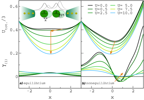
Figure 1: Total potential $\mathcal{U}_{\rm tot.}$ and friction $\gamma$ in 2BA as function of $x$ for different interaction strengths $U$ in (a) equilibrium with $v_{c}=0$ and (b) at finite bias $V_{L}=-V_{R}=5$ with $v_{c}=1$. The system parameters are: $g=1.58$, ${J}_{c}=-3.5$, $J=50$ and ${J}_{\rm tun.}=-8.66$. The inset shows a dimer (green circles) coupled to leads, the effective energy of sites 1 and 2 (horizontal tracts) and the charge density (lines over the dimer) for $x=0$ (solid lines) and for $x>0$ (dashed lines).

In Fig. 1 we plot the total potential $\mathcal{U}_{\rm tot.}=\mathcal{U}_{\rm cl.}+\mathcal{U}_{\rm ss}$ where $\mathcal{U}_{\rm ss}=-\int^{x}_{-\infty}F^{\rm ss}dx$ and friction coefficient $\gamma=\gamma_{11}$, both calculated within the 2BA conserv . In equilibrium, hence $V_{\rm L/R}=0$, the system is symmetric under the inversion of $x$ and so are potential and friction, see panel a). For $U=0$ we have a double minimum in $\mathcal{U}_{\rm tot.}$ corresponding to the two degenerate Peierls-distorted ground states. With increasing $U$ the repulsive-energy cost of the charge-unbalanced Peierls states becomes larger than the distortion-energy gain. Consequently, $\mathcal{U}_{\rm tot.}$ develops a single minimum in $x=0$ and the charge-balanced ground state becomes favored. Independently of $U$, the friction remains positive, an exact equilibrium property correctly captured by our diagrammatic 2BA.

Turning on a gate voltage $v_{c}=1$ and a bias $V_{\rm L}=-V_{\rm R}=5$, see panel b), electrons start flowing through the dimer. The noninteracting formulation predicts self-sustained van der Pol oscillations Bode2011 ; Bode2012 ; Kartsev2014 since the minimum in $\mathcal{U}_{\rm tot.}$ occurs for values of $x$ where $\gamma$ is negative. Thus, the electrical current activates an ever lasting sloshing motion of the dimer. Electron correlations shift the position of the potential minimum away from the region $\gamma<0$, thus hindering the van der Pol oscillations. This effect is even enhanced by the flattening of $\gamma$ that causes a shrinking of the region of negative friction. We point out that the HF approximation, i.e., $\Sigma_{\rm corr.}=0$, predicts the opposite behavior. To validate the correctness of the 2BA treatment we have evaluated $\gamma$ also within the T-matrix approximation conserv (TMA), which accounts for multiple scattering of electrons, and found similar results (see SM).

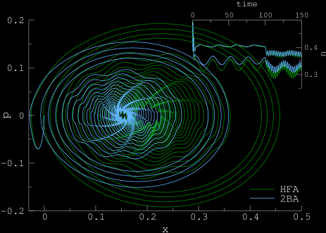
Figure 2: Phase space $(p,x)$ trajectories in ED+GKBA with gate $v_{c}(T)=\theta(T)[1+{\sin}^{2}(\frac{2\pi}{5}2gT)]$ and $U=2.5$ in the HF and 2B approximations (time rescaled by $1/(2g)$). The inset (top right) shows the density of the two sites of the dimer.

The differences between the HF and 2BA results are illustrated in time domain in Fig. 2 using the ED+GKBA approach. We start from an equilibrium situation and then switch on a bias $V_{\rm L}=-V_{\rm R}=5$ and a gate $v_{c}=1$. Then, after time $t=100$, we add a high-frequency time-dependent gate whose only effect is to modulate the nuclear trajectory; ultrafast field have only a minor influence in steering molecular motors. Notice that, although $U/J_{c}\approx 0.7$ (weakly correlated regime), the HF and 2BA trajectories are quantitatively very different.

The effects of Coulomb interactions on the electromechanical energy conversion is investigated in Fig. 3. In the left panels we consider a steady-state system with a bias at time $t=0$ and then suddenly change the position of the nuclear coordinate to $x=0.3$. No external fields other than the bias are switched on, so all quantities depend on time only through $x$. Simulations are performed with ED+ssGF and ED+GKBA (the maximum propagation time is too long for ED+KBE). The nuclear coordinate and site densities show an excellent agreement between the two schemes up to $U=5$. The real-time simulations confirm the conclusions drawn by inspection of Fig. 1. van der Pol oscillations are ever lasting only for $U=0$ [panel a)]; for $U>0$ the dynamics is damped [panels c)-e)]. We can estimate the size of the effect for a normal mode with period $T=2\pi/\Omega\simeq 10^{1}$ fs (hence $V_{L}-V_{R}=10\hbar\Omega\simeq 1\div 10$ eV). In this case the average current through the dimer is in the $\mu$A range (which is congruous for molecular transport) and the amplitude of the sloshing motion is, from Fig. 3, of the order $l_{0}\simeq 10^{-1}\div 10^{-2}~{}{\rm\AA}$ (we assumed a dimer of mass $M\sim 25M_{\rm proton}$ which is appropriate for molecules like, e.g., ethylen). Then for $U=5\hbar\Omega\simeq(0.1\div 1)$ eV the Coulomb-induced damping occurs on the picosecond timescale (see also SM for details).

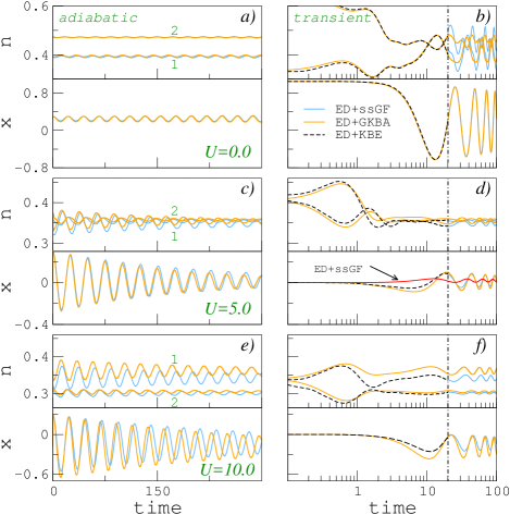
Figure 3: Comparison between ED+GKBA and ED+ssGF for nuclear coordinate and dimer densities in the 2B approximation (time rescaled by $1/(2g)$).

In the right panels of Fig. 3 we explore the performance of the ED+ssGF scheme for a situation when the system has not yet attained a steady state. At time $t=0$ we switch-on a constant (in time) gate $v_{c}=1$ and bias $V_{\rm L}=-V_{\rm R}=5$ and propagate the system using both ED+KBE and ED+GKBA. After a transient phase [time window $(0,20)$] we continue the ED+KBE propagation using the ssGF scheme with initial condition given by the ED+KBE value of the nuclear coordinate at time $t=20$. The duration of the transient phase was chosen longer than the tunneling time in order to wash out the effects of the sudden switch-on of the external fields.

In the noninteracting case, panel b), the system is in a strong nonadiabatic regime, and the ssGF densities are largely deviating from the GKBA densities, especially close to the maxima of $|\dot{x}|$. Nevertheless, the ssGF and GKBA nuclear coordinates are almost identical. This is a consequence of the fact that also the density deviations on the two sites are almost identical, and hence the electronic force (which depends on the densities difference) is not affected by these deviations.

For $U=5$, panel d), the system is in the adiabatic regime after the transient, and we observe a good agreement between the ED+GKBA and the ED+ssGF dynamics. To appreciate the importance of nonadiabatic effects we also plot the result of the pure ED+ssGF dynamics (red line). During the transient ED+ssGF is not expected to work since we are not close to the KBE steady state. Interestingly, however, the impact of the sudden switch-on is strong also at long times; the ED+ssGF nuclear coordinate disagrees considerably from that of ED+GKBA. Increasing the interaction further, panel f), the ED+GKBA dynamics starts to deviate from the ED+KBE dynamics, with a sizable overestimation of the amplitude of the oscillations. This is again a consequence of the failure of the GKBA for too strong $U$’s.

V Conclusions

We introduced a theoretical description of molecular motors in molecular junctions, based on a coupled quantum-classical approach, with nuclei treated within the Ehrenfest dynamics (ED), and electrons within the two-times Kadanoff-Baym Equations (KBE) or the one-time Generalized Kadanoff-Baym Ansatz (GKBA).

In the adiabatic limit of these descriptions, we used the steady-state nonequilibrium Green’s function (ssGF) to derive an expression for the electronic friction coefficient which includes correlation effects due to Coulomb repulsions among the electrons. The adiabatic assumption allows for integrating out the electronic degrees of freedom thus providing a description of the nuclear dynamics in terms of forces that can be calculated and stored in advance. We demonstrated that the proposed ED+ssGF approach is accurate and computationally more efficient than ED+KBE and even ED+GKBA.

We considered the paradigmatic Hubbard dimer to investigate the role of correlations and performed calculations in the mean-field HF approximation as well as in the correlated 2BA and TMA to treat the Coulomb interaction. Numerical evidence indicates that the HF approximation is not accurate enough and that correlation effects can change dramatically the physical picture. In fact, in a broad range of model parameters we found that correlations hinder the emergence of regions of negative friction and strongly damp the nuclear motion. Our results also suggest that fast driving fields play a minor role in designing molecular motors.

Of course, the investigation of electronic correlations in molecular motors is still at its infancy. The proposed ED+ssGF approach allows for standard diagrammatic approximations and therefore well suited for first-principle treatments of realistic setups. We envisage its use to gain insight into molecular devices, and hopefully to put technological applications at a closer reach.

- (1) R. Landauer, J. El. Mat., 4, 813 (1975), and IBM memorandum (1954), unpublished.
- (2) C. Bosvieux and J. Friedel, J. Phys. Chem. Solids 23, 123 (1962).
- (3) J.R. Black, IEEE Trans. Elec. Dev. 16, 338 (1969).
- (4) I. Blech: J. Appl. Phys., 47, 1203 (1976).
- (5) C. Durkan, M. A. Schneider, M. E. Welland, J. Appl. Phys., 86, 1280(1999).
- (6) R. S. Sorbello, Solid State Physics 51, 159 (1997).
- (7) T. N. Todorov, J. Hoekstra, and A. P. Sutton, Phys. Rev. Lett. 86, 3606 (2001).
- (8) E. G. Emberly and G. Kirczenow, Phys. Rev. B 64, 125318 (2001).
- (9) M. Di Ventra, S. T. Pantelides and N. D. Lang, Phys. Rev. Lett. 88, 046801 (2002).
- (10) M. Brandbyge, K. Stokbro, J. Taylor, J. L. Mozos, and P. Ordejon, Phys. Rev. B 67, 193104 (2003).
- (11) M. Cizek, M. Thoss and W. Domcke, Phys. Rev. B 70, 125406 (2004).
- (12) P. S. Cornaglia, H. Ness, and D. R. Grempel, Phys. Rev. Lett. 93, 147201 (2004).
- (13) T. Frederiksen, M. Brandbyge, N. Lorente and A.-P. Jauho, Phys. Rev. Lett. 93, 256601 (2004).
- (14) M. Paulsson, T. Frederiksen, and M. Brandbyge, Phys. Rev. B 72, 201101(R) (2005).
- (15) T. Frederiksen, M. Paulsson, M. Brandbyge and A. P. Jauho, Phys. Rev. B 75, 205413 (2007).
- (16) M. Galperin, A. Nitzan and M. A Ratner, J. Phys. Condens. Matter 19, 103201 (2007).
- (17) M. Galperin, A. Nitzan and M. A Ratner, J. Phys. Condens. Matter 20, 374107 (2008).
- (18) R. Hartle, C. Benesch, and M. Thoss, Phys. Rev. Lett. 102, 146801 (2009).
- (19) R. Zhang, I. Rungger, S. Sanvito and S. Hou, Phys. Rev. B 84, 085445 (2011).
- (20) A. P. Horsfield, D. R. Bowler, and A. J. Fisher, J. Phys. Condens. Matter 16, L65 (2004).
- (21) A. P. Horsfield, D. R. Bowler, A. J. Fisher, T. N. Todorov and C. G. Sánchez, J. Phys. Condens. Matter 16, 8251 (2004).
- (22) C. Verdozzi, G. Stefanucci and C. O. Almbladh, Phys. Rev. Lett. 97, 046603 (2006).
- (23) C. Sanchez, M. Stamenova, S. Sanvito, D.R. Bowler, A.P. Horsfield, and T. Todorov, J. Chem. Phys. 124, 214708, (2006).
- (24) M. Todorovic and D. R. Bowler, J. Phys. Condens. Matter 23, 345301 (2011).
- (25) K. F. Albrecht, H. Wang, L. Muhlbacher, M. Thoss and A. Komnik, Phys. Rev. B 86, 081412 (2012).
- (26) M. Di Ventra, Y.-C. Chen, and T. N. Todorov, Phys. Rev. Lett. 92, 176803 (2004)
- (27) D. Dundas, E. J. McEniry and T. N. Todorov, Nat. Nanotech. 4, 99 (2009).
- (28) T. N. Todorov, D. Dundas and E. J. McEniry, Phys Rev. B 81, 075416 (2010).
- (29) R. Hussein, A. Metelmann, P. Zedler and T. Brandes, Phys. Rev. B 82, 165406 (2010).
- (30) J. T. Lu, P. Hedegard and M. Brandbyge, Phys. Rev. Lett. 107, 046801 (2011).
- (31) J. T. Lu, M. Brandbyge, P. Hedegard, T. N. Todorov and D. Dundas, Phys. Rev. B 85, 245444 (2012).
- (32) J. T. Lu, M. Brandbyge and P. Hedegard, NanoLett. 10, 1657 (2010).
- (33) N. Bode, S. V. Kusminskiy, R. Egger and F. von Oppen, Phys. Rev. Lett. 107, 036804 (2011).
- (34) N. Bode, S. V. Kusminskiy, R. Egger and F. von Oppen, Beilstein J Nanotechnol. 3, 144-162 (2012).
- (35) S. D. Bennett and A. A. Clerk, Phys. Rev. B 74, 201301 (2006).
- (36) J. T. Lu, R. B. Christensen, J.-S. Wang, P. Hedegard and M. Brandbyge, Phys. Rev. Lett. 114, 096801 (2015).
- (37) W. Dou, G. Miao and J.E. Subotnik, Phys. Rev. Lett. 119, 046001 (2017).
- (38) W.Dou and J.E. Subotnik, Phys. Rev. B 97, 064303 (2018).
- (39) F. Chen, K. Miwa and M. Galperin, arXiv:1803.05440 (2018).
- (40) H. L. Calvo, F. D. Ribetto and R. A. Bustos-Marún, Phys. Rev. B 96, 165309 (2017).
- (41) A. Metelmann and T. Brandes, Phys Rev. B 84, 155455 (2011).
- (42) A. Nocera, C. A. Perroni, V. Marigliano Ramaglia and V. Cataudella, Phys. Rev. B 83, 115420 (2011).
- (43) A. Kartsev, C. Verdozzi, G. Stefanucci, EPJ B 87, 14 (2014).
- (44) L.P. Kadanoff and G. Baym, Quantum Statistical Mechanics (Benjamin, New York, 1962).
- (45) L.V. Keldysh, Sov. Phys. JETP 20, 1018 (1965).
- (46) G. Stefanucci and R. van Leeuwen, Nonequilibrium Many-Body Theory of Quantum Systems: A Modern Introduction (Cambridge University Press, Cambridge, 2013).
- (47) K. Balzer and M. Bonitz, Nonequilibrium Green’s Functions Approach to Inhomogeneous Systems, Lecture Notes in Physics Vol. 867 (Springer, Berlin, Heidelberg, 2013).
- (48) M. Hopjan and C. Verdozzi, First Principles Approaches to Spectroscopic Properties of Complex Materials (Springer, Berlin, Heidelberg, 2014); pp.347-384.
- (49) N Schlünzen, J.P. Joost, M. Bonitz, Phys. Rev. B 96, 117101 (2017).
- (50) K. Balzer, N. Schlünzen and M. Bonitz, Phys. Rev. B 94, 245118 (2016).
- (51) E. Boström, M. Hopjan, A. Kartsev, C. Verdozzi and C.-O. Almbladh, J. Phys.: Conf. Ser. 696, 012007 (2016)
- (52) P. Lipavsky, V. Spicka, and B. Velicky, Phys. Rev. B 34, 6933 (1986).
- (53) See Supplemental Material at [URL will be inserted by publisher] for details.
- (54) G. Baym and L. P. Kadanoff, Phys. Rev. 124, 287 (1961).
- (55) M. Puig von Friesen, C. Verdozzi, and C.-O. Almbladh, Phys. Rev. Lett. 103, 176404 (2009); Phys. Rev. B 82, 155108 (2010).
- (56) S. Hermanns, K. Balzer, and M. Bonitz, Phys. Scr. T151, 014036 (2012).
- (57) S. Latini, E. Perfetto, A.-M. Uimonen, R. van Leeuwen, G. Stefanucci, Phys. Rev. B 89, 075306 (2014).
- (58) For , the formulations are equivalent Dou2018 . For , the equivalence could be proven using an exact many-body solution. This is beyond the scope of this work.
- (59) The present treatment correctly reduces to the non-interacting case for and .
- (60) In the spirit of a steady-state density-functional theory (DFT) Stefanucci2015 ; Karlsson2016 ; Kurth2017 ; Karlsson2017 , correlation effects can in principle also be described in terms of exchange-correlation (XC) potential and bias (,). In practice, this can be very challenging, due the difficulty to determine the dynamical exchange-correlations correction to the bias in the leads, due to the evolution of . It thus seems preferable to rely on approximate self-energy schemes as done here rather than make use of DFT.
- (61) G. Stefanucci and S. Kurth, Nano Lett. 15, 8020-8025 (2015).
- (62) D. Karlsson and C. Verdozzi, J. Phys. conf. Ser. 696, 012018 (2016).
- (63) S. Kurth and G. Stefanucci, J. Phys: Cond. Matter, 29 (2017).
- (64) D. Karlsson, M. Hopjan, and C. Verdozzi, Phys. Rev. B 97, 125151 (2018).
- (65) E. Wigner, Phys. Rev. 40, 749 (1932).
- (66) J. Moyal, Proc. Cambridge Philos. Soc. 45, 99 (1949).
- (67) W. Botermans and R. Malfliet, Phys. Rep. 198, 115 (1990).