The SDSS-IV extended Baryon Oscillation Spectroscopic Survey: Baryon Acoustic Oscillations at redshift of 0.72 with the DR14 Luminous Red Galaxy Sample

Abstract

The extended Baryon Oscillation Spectroscopic Survey (eBOSS) Data Release 14 sample includes 80,118 Luminous Red Galaxies. By combining these galaxies with the high-redshift tail of the BOSS galaxy sample, we form a sample of LRGs at an effective redshift $z=0.72$, covering an effective volume of 0.9 Gpc³. We introduce new techniques to account for spurious fluctuations caused by targeting and by redshift failures which were validated on a set of mock catalogs. This analysis is sufficient to provide a $2.6$% measurement of spherically averaged BAO, $D_{V}(z=0.72)=2353^{+63}_{-61}(r_{d}/r_{d,\rm{fid}})$$h^{-1}$ Mpc, at 2.8$\sigma$ of significance. Together with the recent quasar-based BAO measurement at $z=1.5$, and forthcoming Emission Line Galaxy-based measurements, this measurement demonstrates that eBOSS is fulfilling its remit of extending the range of redshifts covered by such measurements, laying the ground work for forthcoming surveys such as the Dark Energy Spectroscopic Survey and Euclid.

=1

1 Introduction

Over the last decade, the expansion history of the Universe has been measured to percent-level precision using observations of the baryon acoustic oscillations (BAO, Peebles & Yu 1970; Sunyaev & Zeldovich 1970; Bond & Efstathiou 1987) in the distribution of galaxies. Multiple measurements from an increasing number of surveys have provided robust support for the standard $\Lambda$CDM cosmological model. Key early surveys such as the Sloan Digital Sky Survey (SDSS; York et al. 2000) and the 2-degree Field Galaxy Redshift Survey (2dFGRS; Colless et al. 2003) generated spectroscopic samples for the BAO measurements given in Eisenstein et al. (2005); Percival et al. (2007) and Percival et al. (2001); Cole et al. (2005), respectively. These spectroscopic programs were followed by the WiggleZ survey at higher redshift (Drinkwater et al., 2010) and the 6-degree Field Galaxy Survey (6dFGS; Jones et al. 2009) at lower redshift, also measuring BAO (Blake et al. 2011a; Beutler et al. 2011, respectively). The Baryon Oscillation Spectroscopic Survey (BOSS; Dawson et al. 2013), conducted as part of the Sloan Digital Sky Survey III (SDSS-III; Eisenstein et al. 2011), provided the first BAO measurements with precision better than 1% (Anderson et al., 2012, 2014a, 2014b; Tojeiro et al., 2014). Results from the final sample of BOSS galaxies were presented in Alam et al. (2017), while results using the final sample of BOSS Lyman-$\alpha$ forests are presented in Bautista et al. (2017) and du Mas des Bourboux et al. (2017).

These BAO measurements are all broadly consistent with a $\Lambda$CDM cosmological model as inferred from Planck satellite measurements (Planck Collaboration I, 2016; Planck Collaboration XIII, 2016). Even so, the low value of the cosmological constant constrained by these data has yet no compelling theoretical explanation (see Weinberg et al. 2013 for a review). The increasing precision of cosmological measurements has renewed the interest in alternative models that predict similar behavior with a different mechanism causing cosmological acceleration (see Clifton et al. 2012 for a review). The combination of BAO measurements with measurements from Redshift-Space Distortions, supernovae, weak-lensing and other low-redshift cosmological probes has therefore recently seen renewed focus, with many planned upcoming experiments. The Taipan survey will observe approximately 2 million galaxies over half the sky at $z<0.4$ (Cunha et al., 2017). At higher redshifts, the Dark Energy Spectroscopic Instrument (DESI; DESI collaboration 2016a, b) and European Space Agency Euclid mission (Laureijs et al., 2011) will observe an order of magnitude more galaxies. The extended BOSS (eBOSS; Dawson et al. 2016), part of the SDSS-IV experiment (Blanton et al., 2017) is the largest spectroscopic galaxy survey running at this time. eBOSS extends the redshift range beyond the BOSS galaxy sample, to redshifts that will be covered by DESI and Euclid.

In this paper we present a BAO measurement at an effective redshift $z=0.72$ using Luminous Red Galaxies (LRGs) observed by eBOSS. This sample, described in Section 2, is designed to extend the CMASS sample from BOSS (Reid et al., 2016) to higher redshift. This sample of galaxies is supplemented by the final BOSS galaxy sample. In addition to the new data, the analysis methods in this work were improved from previous BOSS studies:

• spurious fluctuations caused by non-cosmological variations in target density are modeled from multiple linear regression;

• enhanced characterization of “redshift failures”, i.e., spectra where the redshift is not measured with sufficient statistical significance;

• corrections for targeting inhomogeneity and spectroscopic incompleteness are applied on the random catalog instead of up-weighting galaxies, thus reducing shot-noise and systematic errors in the two dimensional correlation function.

The structure of the paper is as follows. Section 2 describes our data and mock catalogs. Our new treatment of photometric systematic errors and redshift failures is presented in section 3.1 and 3.2, and tested using mock catalogs. The model for BAO in the correlation function and the technique for reconstructing integrated bulk flows that degrade the BAO feature are presented in section 4. Section 5 shows results on data and the main BAO measurement. Table 1 presents the cosmological models employed in our work.

Table 1: Cosmological parameters used in this work.

	Fiducial	Mocks
$\Omega_{M}h^{2}$	0.1417	0.1421
$=\Omega_{c}h^{2}$	0.1190	0.1196
$+\Omega_{b}h^{2}$	0.0220	0.0225
$+\Omega_{\nu}h^{2}$	0.0006	0
$h$	0.676	0.7
$N_{\nu}$	3	3
$\sigma_{8}$	0.8	0.816
$n_{s}$	0.97	0.97
$r_{d}$ [Mpc]	147.78	147.13
$D_{H}(z=0.71)/r_{d}$	20.06	19.82
$D_{M}(z=0.71)/r_{d}$	17.68	17.31
$D_{V}(z=0.71)/r_{d}$	16.45	16.15

2 Data

The sample of galaxies used in this work is mainly composed of Luminous Red Galaxies (LRGs) observed spectroscopically during the first two years of the Extended Baryon Oscillation Spectroscopic Survey (eBOSS, Dawson et al. 2016) — the cosmological component of the fourth generation of the Sloan Digital Sky Survey (SDSS-IV, Blanton et al. 2017). In order to increase tracer density, we combine the eBOSS sample with the $z>0.6$ BOSS CMASS galaxies (Alam et al., 2017) trimmed to the area covered by eBOSS observations. These BOSS galaxies represent about a third of the full sample. These data are found in the SDSS Data Release 14 (Albofathi et al., 2017).

2.1 Galaxy sample and redshift estimators

The eBOSS spectroscopic targets were selected from optical (SDSS DR13, SDSS Collaboration 2016) and infrared (from the Wide-field Infrared Survey Explorer, WISE, Wright et al. 2010) imaging data with infrared forced photometry applied over positions of SDSS sources (Lang et al., 2014). The LRG target selection is fully described in Prakash et al. (2016). The selection algorithm was informed by Prakash et al. (2015) and applied over the full BOSS imaging footprint, yielding about 60 deg^-2 LRG targets, of which 50 deg^-2 were observed spectroscopically. In short, the main (extinction corrected) SDSS magnitude cuts of this sample are given by

$$z<19.95\ \ \ \ 19.9<i<21.8$$ (1)

which makes the eBOSS LRG galaxies a completely disjoint set (in magnitudes, not redshift) from CMASS galaxies (Eisenstein et al., 2011). Additional color cuts,

$$r-i>0.98\ \ \ \ i-z>0.625\ \ \ \ r-W1>2(r-i),$$ (2)

yield, on average, higher redshift galaxies than CMASS while avoiding star contamination. The selection was tested over 466 deg² covered during the Sloan Extended Quasar, ELG, and LRG Survey (SEQUELS). An overview of this pilot survey can be found in Dawson et al. (2016) and in the DR12 data release (Alam et al., 2015a).

Spectra were obtained by the Sloan 2.5m telescope at Apache Point Observatory, New Mexico, USA (Gunn et al., 2006). Two multi-object spectrographs (Smee et al., 2013) simultaneously project 1000 spectra per exposure, including about 20 calibration stars and $\sim 80$ empty regions (for modeling sky subtraction). Spectra cover a wavelength range from 3,600 to 10,000 Å with a resolution $R=1500-2600$. Sets of 15 minute exposures were taken until a typical target with $g=21.2$ and $i=20.2$ reaches a signal-to-noise ratio of 3.16 per pixel in the $g$ band and 4.7 per pixel in the $i$ band.

Spectra were extracted, sky-subtracted, flux-calibrated and co-added using version v5_10_0 of the software idlspec2d. The extraction algorithm has improved since BOSS, its description can be found in Appendix B of Bautista et al. (2017). Recent improvements on co-addition and flux-calibration are described in Hutchinson et al. (2016) and Jensen et al. (2016). The final eBOSS LRG spectra were classified and their redshifts measured primarily by redmonster (Hutchinson et al., 2016), complemented by redshifts obtained using spec1d (Bolton et al., 2012). On average 10% of the eBOSS LRG sample lacks a statistically confident redshift estimate due mainly to the low signal-to-noise ratio of their spectra. In section 3.2 we discuss how to this failure rate depends on many characteristics of the observations, e.g., position of the fiber in the focal plane or position of the trace in the CCD. In that section we present the methods used to account for these fluctuations in our clustering measurement.

2.2 Catalog creation

One important step of the clustering analysis is to determine the survey mask. Usually the mask is defined by a set of random points Monte-Carlo sampling the volume covered by the survey, referred as the “random catalog” or simply “the randoms”. This random catalog also accounts for angular variations in spectroscopic completeness of the survey. We follow here a similar procedure to that used for the final BOSS galaxy clustering measurements, described in Reid et al. (2016).

Starting from the photometric target sample, we first veto objects in “bad” photometric regions of the sky which were included in the target selection process. We exclude regions around stars in the Tycho catalog (Høg et al., 2000) with Tycho $B_{T}$ magnitudes within [6, 11.5] with a magnitude-dependent radius ranging from 3.4^′ to 0.8^′. An additional mask excludes regions 0.1 to 1.5^∘ in radius around bright galaxies and other objects (Rykoff et al., 2014). Bright objects in WISE imaging are also masked. Regions of radius from 16.6^′ to 2^′ are masked around sources with W1 magnitudes ranging from 2 to 8. We removed regions where galactic extinction $E(B-V)>0.15$ or where the seeing is larger than 2.3, 2.1, 2.0^′ in $g$, $r$ and $i$ bands, respectively. Bad photometric regions and bright objects mask 4.5% of the targets in the NGC and 12.1% of targets in the SGC. Since the eBOSS quasars and several other target classes have priority during the fiber assignment procedure (Dawson et al., 2016), we are unable to obtain spectra from LRG targets that lie less than 62^′′ (corresponding angular diameter of a fiber in the sky) from a higher priority target. This results in 7.7% of LRG targets being masked by quasar fibers in the NGC and 7.0% in the SGC. We expect that the effect on the LRG clustering caused by these knockouts is negligible given that other sample are relatively sparse and have little overlap in redshift with the galaxy sample. We leave tests on this assumption to future work. We mask few tens of the remaining LRG targets that lie in the center of the focal plane, where a center post holds the plate and prevents fibers from being assigned within the 92^′′ central radius. The total masked area is 12.3% for the NGC and 18.2% for the SGC. Targets that are masked in this process do not account in the fiber completeness calculations (see below).

The spectroscopic sample is then matched to the remaining targets. A small fraction of targets do not receive an optical fiber and therefore have no spectra or redshift information. Some of these missing redshifts are caused by the impracticability of placing two optical fibers on LRG targets closer than 62^′′. We refer to these as fiber collisions. These collisions impact the small-scale clustering since they preferably occur in over-dense regions. Different methods to correct for the effect of collisions have been studied in the past (e.g., Guo et al. 2012; Bianchi & Percival 2017). For our catalogs, we simply up-weight by one the target with redshift information as performed in Alam et al. (2017). The impact on correlations larger than 10$h^{-1}$ Mpc is negligible (Guo et al., 2012). Other targets do not receive a fiber because of the limited number of fibers available per observation (1000 fibers).

We correct for these missing targets by downsampling the random catalog so it follows the computed completeness. We define fiber assignment completeness as:

$$C=\frac{N_{\rm gal}+N_{\rm qso}+N_{\rm star}+N_{\rm cp}+N_{\rm fail}}{N_{\rm targ}}$$ (3)

where $N_{\rm gal}$ is the number of confirmed LRGs with redshifts, $N_{\rm qso}$ and $N_{\rm star}$ are the numbers of quasars and stars found among LRG targets (incorrect target classes), $N_{\rm cp}$ is the number of LRG targets without spectra due to a collision with a galaxy with a redshift (they count as being observed), and $N_{\rm fail}$ is the number targets with spectra but without a confident redshift (we correct for redshift failures in a later process, see Section 3.2). The fiber completeness is computed per “sector”, where a sector is a connected region of the sky defined by a unique set of plates. We exclude sectors where the fiber completeness is below 50% to avoid regions covered by multiple plates, where unfinished observations potentially introduce an artificial pattern of clustering.

Fig. 1 displays the footprint of the DR14 LRG sample where the color-coding indicates the corresponding fiber completeness. The top of Table 2 presents the number of LRGs, the total effective area (weighted by completeness) of our sample and the effective volume (defined below) of our samples.

Table 2: Survey specification of the eBOSS LRG sample used in this analysis

Survey	Cap	$N_{\rm gal}$	$N_{\rm zfail}$	$N_{\rm cp}$	$N_{\rm qso}$	$N_{\rm star}$	$A_{\rm eff}$ [deg2]	$V_{\rm eff}\ [{\rm Gpc}^{3}]$
	NGC	45826	4957	2263	18	2897	1033.4	0.356
eBOSS	SGC	34292	4366	1687	18	4273	811.6	0.262
	Total	80118	9323	3950	36	7170	1844.0	0.618
eBOSS +	NGC	71975						0.511
CMASS	SGC	54582						0.389
$(0.6<z<1.0)$	Total	126557						0.900

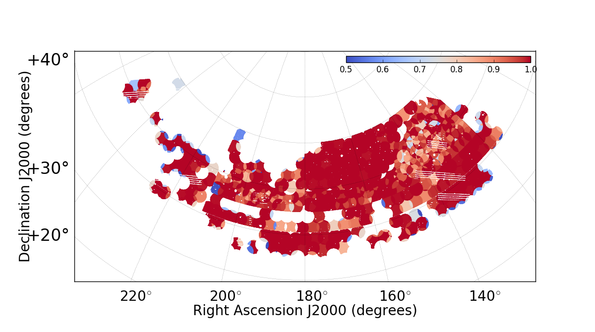
Figure 1: The footprint of the DR14 LRG sample. The colors show the fiber completeness per region for the eBOSS sample only. Regions with fiber completeness below 0.5 were removed from the final sample.

Using the fiducial cosmology presented in Table 1, we compute weights that optimize clustering signal-to-noise for a survey with varying density as a function of redshift. Also known as FKP weights (Feldman, Kaiser, & Peacock, 1994), we apply a weight to each object,

$$w_{\rm FKP}=\frac{1}{1+\bar{n}(z)P_{0}},$$ (4)

where $\bar{n}(z)$ is the average comoving density of galaxies as a function of redshift and $P_{0}$ is the value of the power spectrum at scales relevant for our study ($k\sim 0.14~{}h$Mpc^-1, Font-Ribera et al. 2014). For the eBOSS LRG sample we adopt a value of $P_{0}=10^{4}~{}h^{-3}{\rm Mpc}^{3}$ which is the same value used in the final BOSS CMASS clustering measurements. The effective volume is defined as

$$V_{\rm eff}=\int_{z=0.6}^{z=1.0}\left(\frac{\bar{n}(z)P_{0}}{1+\bar{n}(z)P_{0}}\right)^{2}{A_{\rm eff}}R^{2}(z){\rm d}R(z),$$ (5)

where $R(z)$ is the comoving distance to redshift $z$ and $A_{\rm eff}$ is the effective area (in steradians) of the survey.

We built the random catalog using a sample 50 times that of the galaxy sample size. We applied the same veto masks as for the observed targets. Redshifts are assigned to each random point such as to match the redshift distribution $\bar{n}(z)$ of the data. Fig. 2 shows the redshift distribution of our samples, separately for the NGC and the SGC. We restrict our analysis to $z>0.6$ to avoid a larger overlap with the CMASS sample while not reducing the effective redshift. The cut at $z<1.0$ was chosen to avoid low number density of LRGs. In section 3, we describe how systematic effects caused by target selection and redshift failures are corrected using the same random catalog.

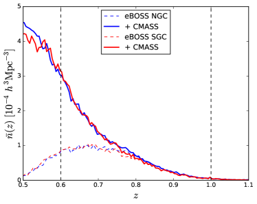
Figure 2: Density of LRGs as a function of redshift. Dashed vertical lines indicate the redshift range used in our clustering measurement. Here we see that a significant fraction of eBOSS LRGs have redshifts below 0.6, where CMASS are more numerous. We can remark the importance of the CMASS sample between redshift 0.6 and 0.7.

2.3 Mock catalogs

We created a set of mock catalogs, each reproducing the angular and redshift distribution of galaxies in the DR14 sample (Fig. 1), as well as the large-scale correlation function predicted from the fiducial cosmology. We produced simulations for both eBOSS and for the combined CMASS+eBOSS sample using redshift distributions shown in Fig. 2.

Mock catalogs were created with the Quick Particle Mesh (QPM) method (White et al., 2014), also used in recent clustering studies (Alam et al., 2017; Ata el al., 2018). Each realization consists of a different set of 2nd order Lagrangian Perturbation Theory (2LPT) initial conditions computed at $z=25$. These perturbations were evolved to $z=0.7$ using a low-force and low-mass resolution particle-mesh N-body simulation, with time steps of 15% in the log of the scale factor. The runs employed here were based on a 2560 $h^{-1}$ Mpc side box containing $1280^{3}$ dark-matter particles. Halos were defined using a friends-of-friends algorithm with a linking length of 20% the mean inter-particle spacing. These halos are populated with galaxies following a Halo Occupation Distribution (HOD) model, derived from the small-scale clustering of the same LRG sample (Zhai et al., 2017). We sub-sample galaxies in order to reproduce the redshift distribution $n(z)$ and the angular fiber-completeness as measured from the data. We introduce redshift failures into our mock catalogs by sampling from the model derived in section 3.2.

3 Correcting non-cosmological density fluctuations

As described in the previous section, eBOSS LRG targets were selected to be strictly fainter in $i$-band magnitudes than the CMASS sample. Larger photometric errors in this regime create a higher rate of contamination by stars and, for some galaxy spectra, scatter from faint galaxies into the selection. Therefore, the eBOSS LRGs are more susceptible to contamination by inhomogeneities in target selection and by patterns in redshift failures than the CMASS galaxies from BOSS. I n this section we introduce methods to account for this contamination. All work in this section is focused on the eBOSS sample only.

3.1 Systematics due to photometry

In BOSS clustering studies, it was found that galaxy density is correlated with stellar density and seeing (Ho et al., 2012; Ross et al., 2011, 2012, 2017). These correlations contaminate our clustering measurements by introducing large-scale power not associated with the true distribution of galaxies. In Ross et al. (2017), systematic weights were computed for each galaxy in order to counteract these dependencies, but assuming different systematics are independent. In this work, we drop the assumption of independent systematics and use a multiple linear regression, similar to that used to assess variations in the target selection of LRGs (Prakash et al., 2016), quasars (Myers et al., 2015) and ELGs (Delubac et al., 2017; Raichoor et al., 2017). The multiple linear regression has the advantage of automatically accounting for correlated systematics, e.g., stellar density and Galactic extinction. In performing the regression, we include only galaxies with confident spectroscopic redshifts in the region of interest $0.6<z<1.0$. The NGC and SGC samples are analyzed independently.

The multiple linear regression calculates a “density” model, $\delta_{\rm phot}$, as a linear combination of maps $m_{i}$:

$$\delta_{\rm phot}({\rm RA,Dec})=p_{0}+\sum_{i=1}^{n}p_{i}m_{i}({\rm RA,Dec}),$$ (6)

where $p_{0}$ is the average density over the full footprint and $p_{i}$ (with $i>0$) are fitted coefficients that minimize $\chi^{2}=(\delta-\delta_{\rm phot})^{2}/\sigma_{\delta}^{2}$. Each map $m_{i}$ is produced using Healpix with pixels of equal area of 189 arcmin². The observed fluctuations $\delta$ are estimated from the data (normalized ratio of number of galaxies and randoms) as a function of a given systematic value. The number of galaxies and randoms in each bin are weighted by $w_{\rm FKP}$ (Eq. 4) in order to account for the cosmological fluctuations. Error bars are assumed to be Poisson on the weighted number of galaxies per bin.

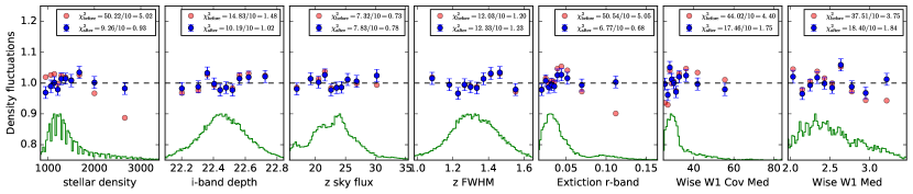
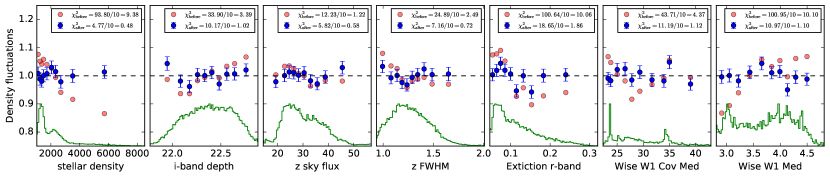
Figure 3: Fluctuations of galaxy number density with respect to different photometric quantities for the NGC (top panels) and the SGC (bottom panels). Red (blue) points indicate fluctuations before (after) corrections. The distribution of the same quantities among galaxies is shown in green. The fit is made simultaneously across all maps, accounting automatically for correlations between different maps.

Fig. 3 shows the result of the regression using seven different maps. Five of these maps are derived from SDSS photometry (Doi et al., 2010; Aihara et al., 2011): stellar density, $i$-band depth, $z$-band sky flux, $z$-FWHM and $r$-band extinction, while two maps are derived from WISE photometry (Wright et al., 2010; Lang et al., 2014): median number of single-exposure frames per pixel in WISE W1 band (WISE W1 Cov Med) and median of accumulated flux per pixel in the WISE W1 band (WISE W1 Med). Since different SDSS bands (Fukugita et al., 1996) are strongly correlated, we restrict our analysis to a single band per systematic. In the NGC, $\chi^{2}/dof=192.2/(70-8)$ before corrections and $80.6/(70-8)$ after corrections, while in the SGC we obtain $\chi^{2}/dof=365.8/(70-8)$ before corrections and $68.2/(70-8)$ after corrections. The most important improvements are related to dependencies with stellar density, extinction and WISE quantities. This analysis can be perfomed in many redshift bins, however, no further improvement was obtained. Hereafter, we compute systematic maps using a single redshift bin.

Once the density model is derived, our sample can, in principle, be corrected either by applying to the galaxies a set of systematic weights defined as $w_{\rm sys}=1/\delta_{\rm phot}$, or by sub-sampling the random catalog as a function of RA and Dec to mimic the density model.

Fig. 4 presents the monopole and the quadrupole of the correlation function calculated using the standard Landy & Szalay (1993) estimator. We show the observed correlation function before accounting for non-cosmological fluctuations in target density and compare the results of correcting with an up-weighting scheme to results from sub-sampling of randoms. Correlations are biased positive even for large separations where no cosmological signal is expected. As we can see in the figure, the quadrupole is barely affected by this kind of systematic error.

Differences between the two correction techniques are smaller than error bars and are consistent with being caused by the relatively smaller number of randoms for the sub-sampling case. Hereafter, targeting systematics are corrected by sub-sampling of randoms.

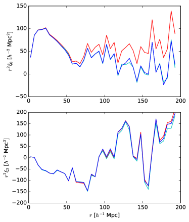
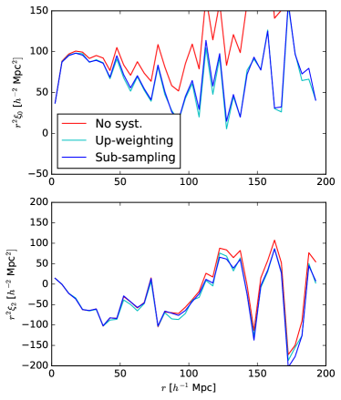
Figure 4: Monopole (top panels) and quadrupole (bottom) of the correlation function for NGC (left) and SGC (right) before (red lines) and after correcting for targeting systematics. The cyan line shows the result when using the up-weighting scheme and the blue line shows the sub-sampling of randoms. Since our corrections for redshift failures are also applied on the random catalog, we employ hereafter the sub-sampling of randoms as our fiducial method to correct for targeting systematics.

3.2 Correcting for redshift failures

Variations in the quality of spectroscopy can have a similar effect on clustering as variations in the quality of the photometry used to identify targets. Fig. 5 reveals that lower S/N spectra yield, on average, fewer statistically confident redshifts. We define redshift efficiency as

$$\eta=\frac{N_{\rm gal}}{N_{\rm zfail}+N_{\rm gal}},$$ (7)

where quantities are defined in Section 2.2. If the expected distribution of failures is not uniformly distributed across the sky, our clustering measurements might be biased. In this section, we introduce a new technique to account for these failures. Using mock catalogs (described in Section 2.3), we demonstrate that our method leads to unbiased clustering measurements.

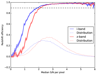
Figure 5: Average redshift efficiency as a function of median pixel signal-to-noise ratio in the $i$ (blue line) and $z$ (red line) SDSS bands. Dotted lines indicate the distribution of median S/N of the eBOSS LRG sample. The dashed line represents the average redshift efficiency of the whole sample of 90.5%.

In previous studies from BOSS, redshift failures were accounted for by an up-weighting technique. These spectra lacking a confident redshift transfer their weight to the nearest object in the sky with a confident redshift (either a galaxy or a star). In other words, the nearest neighbor of a failure will count double when counting pairs. This simple correction procedure leads to unbiased results on scales far larger that the average separation between a failure and a non-failure and as long as the rate of redshift failures is low. For example, in the BOSS CMASS sample the overall failure rate was 1.8% and the median separation was 3.8 arcmin. In the eBOSS LRG sample, the failure rate is around 10% and the median separation is 5 arcmin. The higher failure rate and larger average separation force us to revisit the manner in which redshift incompleteness is addressed in eBOSS.

Instead of using the up-weighting technique, we derive a model describing the probability of an observation of a target galaxy yielding a confident redshift. In our model, this probability depends on the the position of its fiber in the focal plane and the overall signal-to-noise ratio of the plate. The model for failures is then applied to the random sample, by sub-sampling, mimicking the patterns retrieved in our model.

Fig. 6 shows the probability of obtaining a confident redshift (hereafter called the redshift efficiency) for a galaxy as a function of its position in the focal plane. We observe a decrease in this probability near the side edges of the focal plane. The reason for this behavior is that the light transmitted through fibers near the side-edges of the focal plane arrive near the edges of the CCD, where the optical performance inside the spectrographs is degraded, leading to a larger point spread function and optical aberrations such as coma (Smee et al., 2013). By associating each random with a plate and location within the plate, we can use the binned probabilities to sub-sample the random catalog. We divide the focal plane into 20 bins across the diameter of the focal plane in cartesian coordinates, XFOCAL and YFOCAL, that range from -326 to 326mm. Our choice of bin size is large enough to minimize Poisson noise in galaxy counts but small enough to identify the failure-rate pattern on the scales of interest.

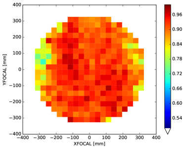
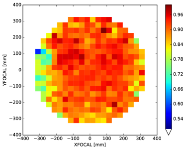
Figure 6: Average redshift efficiency as a function of physical position of the optical fiber in the focal plane. Left (resp. right) panel shows the NGC (resp. SGC) failure rates. The region where YFOCAL is negative correspond to spectrograph #1 while YFOCAL $>0$ corresponds to spectrograph #2.

Fig. 7 presents this dependency of the redshift efficiency with signal-to-noise ratio of both spectrographs for each plate. We use these half-plates since two independent spectrographs have different throughput (Smee et al., 2013). On average, fibers lying on the YFOCAL$<0$ region (in Fig. 6) encounter spectrograph #1, while the others are typically imaged through spectrograph #2. Independent measurements of $S/N$ are made per spectrograph and per optical band (corresponding to SDSS $g$, $r$, $i$). We used $i$ band values only, given that most of the signal of LRG spectra is observed in the $i$ band. The binned data (blue points) are included in order to reduce Poisson noise. We fit the efficiency $\eta$ using a simple model,

$$\eta(x)=\frac{1}{1+1/p(x)},$$ (8)

where $x=(S/N)^{2}$ and $p(x)$ is a first order polynomial. This choice of model ensures the correct asymptotic behavior when $S/N\rightarrow 0$ or $S/N\rightarrow\infty$. The best-fit models yield $\chi^{2}/{\rm dof}=47.1/(20-2)$ for the NGC, and $\chi^{2}/{\rm dof}=39.2/(20-2)$ for the SGC. These values are higher than unity, indicating that efficiencies may depend on factors other than spectrograph $S/N$. However, we were not able to identify any other significant factors. We expect to improve the model of redshift failures with a larger data sample.

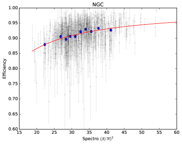
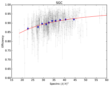
Figure 7: Average redshift efficiency per spectrograph as a function of its signal-to-noise ratio squared binned (blue points) and unbinned (gray points). Red line show the best-fit models. The left panel shows the results for the NGC while the right panel shows the SGC. Signal-to-noise is computed as the median per pixel over the i-band wavelength range.

Our final efficiency model is the product of the two efficiencies given in Fig. 6 and Eq. 8. We normalize the efficiencies such that the final product is consistent with the average spectrograph efficiency given by the red line in Fig 7 (since the latter already includes the average focal plane efficiencies).

The sub-sampling technique is implemented as follows. For each random galaxy, we assign a plate, XFOCAL and YFOCAL values based on its location in the sky. In overlap regions covered by more than a single plate, a random plate value among those observing this region is assigned to this random galaxy. Given the plate number and the (RA, Dec) of each random, we can assign a position in the focal plane of that plate. We draw random numbers and we remove random galaxies based on the probability given by the model.

In order to test our procedure, we included redshift failures on the set of 1000 mock catalogs for eBOSS galaxies, following the model derived from real data. We first assign mock galaxies to plates (and their XFOCAL and YFOCAL) as done with the randoms. For each galaxy, we randomly convert it as a failure based on the probability given by the model. We apply two methods to account for these failures: the nearest-neighbor up-weighting and the sub-sampling of randoms. For the sub-sampling case, we use redshift failures from the mock itself to derive individual redshift efficiency models, employing the same algorithm that is used to derive the inefficiency model from the data. Doing so accounts for the Poisson noise that could be caused by the binned data.

Fig 8 shows the impact of different correction methods on the average correlation function of the 1000 mock catalogs. The reference correlation function is computed from the same mock catalogs without any synthetic redshift failures. The grey region represents the error on the mean of 1000 correlation functions (all curves have similar errors). The nearest-neighbor up-weighting scheme (blue curve) introduces structure into the monopole with amplitude smaller than the error on the 1000 mocks, except at scales below 20$h^{-1}$ Mpc which are usually discarded in BAO analyses. However, this scheme introduces a bias of at least 5% on all scales in the amplitude of the quadrupole. The sub-sampling technique (green lines) has better performance than up-weighting for all scales, for both monopole and quadrupole, yielding no significant bias at this level of precision. We also applied two “non-complete” versions of the sub-sampling scheme, where we assume the efficiency model depends only on one factor: either focal plane position or only spectrograph $S/N$. Even when our assumed model for redshift failures is not complete, our model is superior to the up-weighting scheme.

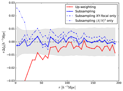
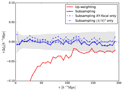
Figure 8: Difference between the average mock correlation function where redshift failures are corrected and the mocks without synthetic failures. The left panel presents the monopole and the right panel shows the quadrupole, both scaled by $r$ for clarity. Different lines present the results with different schemes. The grey band is the error on the mean of 1000 mock catalogs of the eBOSS NGC sample (without CMASS). The up-weighting of nearest neighbor technique introduces a bias of 5% in the quadrupole on all scales while the sub-sampling is unbiased.

The bias on the quadrupole introduced by up-weighting would yield biased estimates of the growth rate of structures in studies of redshift-space distortions. We recommend that future work on RSD using galaxy samples containing significant failure rates implement our correction scheme.

We use the sub-sampling techniques on the eBOSS LRG sample in all clustering measurements in this work. For the CMASS $z>0.6$ sample we employ the weights used in the final BOSS measurements, which use the up-weighting technique. We combine CMASS and eBOSS samples, both data and randoms, making sure that the ratio of number of galaxies over randoms is the same.

4 The model and fitting methodology

In this section, we describe the model used to fit the correlation function, the reconstruction procedure applied, and tests on the mock catalogs.

4.1 The model

To fit the measured correlation function we follow the standard approach described in previous papers (e.g., Alam et al. 2017; Ata el al. 2018). The model redshift-space correlation function is obtained from a Fourier transform of the power-spectrum, which is defined as

$$P(k,\mu)=\frac{b^{2}\left[1+\beta(1-e^{-k^{2}\Sigma_{r}^{2}/2})\mu^{2}\right]^{2}}{(1+k^{2}\mu^{2}\Sigma_{s}^{2})}\left[P_{\rm lin}(k)+P_{\rm peak}(k)\left(e^{-k^{2}\Sigma_{\rm nl}^{2}(\mu)}-1\right)\right]$$ (9)

where $b$ is the linear bias, $\beta$ is the redshift-space distortions parameter, $k$ is the modulus of the wave-vector and $\mu$ is the cosine of the angle between the wave-vector and the line-of-sight. We introduce anisotropic non-linear broadening of the BAO peak by multiplying the “peak-only” power spectrum $P_{\rm peak}$ by a Gaussian term with $\Sigma_{\rm nl}^{2}(\mu)=\Sigma_{\parallel}^{2}\mu^{2}+\Sigma^{2}_{\perp}(1-\mu^{2})$. The non-linear random motions on small scales are modeled by a Lorentzian term parametrized by $\Sigma_{s}$. Typical values for the damping terms can be computed by fitting the average of many mocks: $(\Sigma_{\parallel},\Sigma_{\perp},\Sigma_{s})=(9.5,6.0,2.0)$ $h^{-1}$ Mpc for pre-reconstruction and $(\Sigma_{\parallel},\Sigma_{\perp},\Sigma_{s})=(5.5,5.5,0)$ $h^{-1}$ Mpc for post-reconstruction. Given the relatively low signal-to-noise ratio of the correlation functions of this sample, all fits have $(\Sigma_{\parallel},\Sigma_{\perp},\Sigma_{s})$ values fixed. Following theoretical motivation of White (2015) and Seo et al. (2016), we apply a term $S(k)=e^{-k^{2}\Sigma_{r}^{2}/2}$ to the post-reconstruction modeling of the correlation function. This term models the smoothing used in our reconstruction technique, where $\Sigma_{r}=15$$h^{-1}$ Mpc (see section 4.3). This term was used in the BOSS DR12 results of Ross et al. (2017) and Beutler et al. (2017a). We follow Kirkby et al. (2013) to compute $P_{\rm peak}$ from the linear power-spectrum $P_{\rm lin}$, by computing its correlation function, fitting a third-order polynomial function over the peak region, and transforming back to Fourier space. The linear power spectrum $P_{\rm lin}$ is computed using the code CAMB (Lewis et al., 2000) with cosmological parameters of our fiducial cosmology (Table 1).

In practice, we derive multipoles for the correlation function $\xi_{\ell}(r)$ from multipoles of the power-spectrum $P_{\ell}(k)$, simply defined as:

$$P_{\ell}(k)=\frac{2\ell+1}{2}\int_{-1}^{1}P(k,\mu)L_{\ell}(\mu)~{}{\rm d}\mu$$ (10)

where $L_{\ell}$ are Legendre polynomials. The correlation function is:

$$\xi_{\ell}(r)=\frac{i^{\ell}}{2\pi^{2}}\int_{0}^{\infty}k^{2}j_{\ell}(kr)P_{\ell}(k)~{}{\rm d}k$$ (11)

where $j_{\ell}$ are the spherical Bessel functions.

In order to measure the BAO peak position, we scale separations $r$ with an isotropic dilation factor, $\alpha_{\rm iso}$, defined as the ratio of the “spherically averaged” distance:

$$D_{V}(z)=[zD_{M}^{2}(z)D_{H}(z)]^{1/3}$$ (12)

to the sound horizon scale $r_{d}$, normalized to its value in our fiducial cosmology, i.e:

$$\alpha_{\rm iso}=\frac{D_{V}(z_{\rm eff})/r_{d}}{D^{\rm fid}_{V}(z_{\rm eff})/r_{d}^{\rm fid}}.$$ (13)

Another choice of parametrization of the BAO peak position uses two dilation parameters that decompose the scaling into transverse, $\alpha_{\perp}$, and radial, $\alpha_{\parallel}$, directions. These quantities are related, respectively, to the comoving angular diameter distance, $D_{M}=(1+z)D_{A}(z)$, and to the Hubble distance, $D_{H}=c/H(z)$, by

$$\alpha_{\perp}=\frac{D_{M}(z_{\rm eff})/r_{d}}{D_{M}^{\rm fid}(z_{\rm eff})/r_{d}^{\rm fid}}\hskip 56.9055pt\alpha_{\parallel}=\frac{D_{H}(z_{\rm eff})/r_{d}}{D_{H}^{\rm fid}(z_{\rm eff})/r_{d}^{\rm fid}}$$ (14)

In our implementation, we apply the scaling factors in the two-dimensional power spectrum (Eq. 9) before computing its multipoles and the associated Hankel transforms (e.g. Beutler et al. 2014; Gil-Marín et al. 2017).

Unknown systematic effects in the survey might create large-scale correlations that could contaminate our measurements. We take into account any spurious correlations by introducing into our model a smooth functions of separation. Our final template can be written as

$$\xi^{t}_{\ell}(r)=\xi_{\ell}(\alpha r)+a_{\ell 0}+\frac{a_{\ell 1}}{r}+\frac{a_{\ell 2}}{r^{2}}.$$ (15)

For isotropic fits, we only fit the monopole of the correlation function, fixing the value of $\beta=0.3$. For anisotropic fits, we fit both monopole and quadrupole, leaving $\beta$ as a free parameter and fitting $b$ with a Gaussian prior of 30% around $b=2.3$. For all fits, the broadband parameters are free while dilation parameters are fitted in the range $0.5<\alpha<1.5$. A total of 5 parameters are fitted on isotropic fits and 10 parameters for anisotropic fits.

4.2 Parameter estimation

The best-model is found by minimizing $\chi^{2}=d\hat{W}d^{T}$, where $d$ is the monopole (and quadrupole) of the correlation function, and $\hat{W}$ is the estimated precision matrix, defined as the inverse of the estimated covariance matrix $\hat{C}$. We use the iMinuit python package that implements a quasi-Newton method using DFP formula to find minima. All of our covariance matrices are derived from the scatter of measurements from mock catalogs. In order to account for the finite number of mock measurements used to derive $\hat{C}$, the unbiased estimator for the precision matrix (Hartlap et al., 2007; Taylor et al., 2014; Percival et al., 2014) should be written as

$$\hat{W}=\left(1-\frac{n}{N_{\rm mocks}-1}\right)\hat{C}^{-1},$$ (16)

where $n$ is the number of elements in the data vector $d$.

Errors from best-fit parameters are derived from the $\Delta\chi^{2}=1$ region of the marginalized $\chi^{2}$ profiles. Errors on the BAO scale $\alpha_{\rm iso}$ are usually asymmetric for the current signal-to-noise ratio of our samples.

4.3 Reconstruction

To reduce the non-linear effects on the BAO feature, we applied “reconstruction” (Eisenstein et al., 2007; Burden, Percival & Howlett, 2015; Vargas-Magaña et al., 2017) to the eBOSS+CMASS sample. The reconstruction method reverses a fraction of non-linear motion of the overdensities, sharpening the BAO peak and thus increasing the precision of our distance-redshift measurement.

Using the Zeldovich approximation, we calculate Lagrangian displacements $\vec{\Psi}$ based on an estimate of the velocities made from the density field. In order to estimate the galaxy density field, we insert the NGC or the SGC region inside a box with width 3.6 comoving $h^{-1}$Gpc, assigning the galaxies and randoms into a grid of $512^{3}$ cells (using our fiducial cosmology). We use the cloud-in-cell scheme to assign galaxies and randoms to the grid. The density is smoothed using a three-dimensional Gaussian kernel with 15$h^{-1}$ Mpc as its characteristic length. Burden et al. (2014); Vargas-Magaña et al. (2017) studied how results vary as a function of this smoothing length and found that 15$h^{-1}$ Mpc is close to optimal in terms of sharpening the BAO peak for densities similar to those matching our samples.

For a redshift-space density field, we find an approximate solution for the displacement field using Inverse Fast Fourier Transforms (IFFT),

$$\vec{\Psi}={\rm IFFT}\left[\frac{-i\vec{k}\tilde{\delta}(\vec{k})}{bk^{2}}\right]-\frac{f}{b+f}\left({\rm IFFT}\left[\frac{-i\vec{k}\tilde{\delta}(\vec{k})}{bk^{2}}\right]\cdot\hat{r}\right)\hat{r},$$ (17)

where $\tilde{\delta}$ is the Fourier transform of the density field, $\vec{k}$ is the wave-vector, $b$ and $f$ are values for the bias and growth rate for the sample, and $\hat{r}$ is the unit vector in the radial direction. Because the overdensity field in redshift-space is not irrotational, this equation is only an approximation, although it can be made more accurate, tending towards the true solution, using an iterative approach (Burden, Percival & Howlett, 2015).

Once the displacement field has been calculated, we move both data and randoms by the expected value to obtain the reconstructed catalogs. We can also remove redshift-space distortions by moving galaxies by an additional displacement defined as

$$\vec{\Psi}_{\rm RSD}=-f(\vec{\Psi}\cdot\hat{r})\hat{r}.$$ (18)

This action does not reduce the signal-to-noise ratio of the reconstructed overdensity field measurement (the transition from real to redshift-space increases the information content).

We consider three implementations of the reconstruction method. The differences between them are whether or not we remove RSD, and how many iterations we perform as in Burden, Percival & Howlett (2015).

• A: Not removing RSD and not performing iterations

• B: Removing RSD and not performing iterations

• C: Removing RSD and performing iterations

For case B, we use Eq. 19 in Burden, Percival & Howlett (2015).

4.4 Fitting mock catalogs

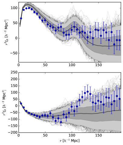
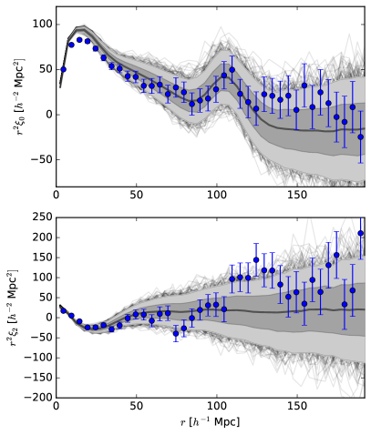
Figure 9: Comparison of the monopole (top panels) and quadrupole (bottom panels) of data (blue points) and mock catalogs (gray lines) of the eBOSS+CMASS combined NGC+SGC. Panels on the left (right) show the pre(post)-reconstruction catalogs. The shaded regions represent the 68 and 95% boundaries of the distributions of correlation functions around the mean. Mocks and data correlation functions agree on most scales, except in the monopole at $r<30$$h^{-1}$ Mpc (excluded from our analysis) and around $r\sim 120$$h^{-1}$ Mpc in the quadrupole.

We computed the correlation function for all 1000 mock catalogs of the eBOSS+CMASS samples, pre and post reconstruction. Our fiducial cosmology was employed to compute comoving separations. The monopoles and quadrupoles for the mock catalogs are displayed in Figure 9 and compared with the data. For scales of interest for BAO ($r>30$$h^{-1}$ Mpc) the mock and data results mostly agree, except on few points in the quadrupole where the data show deviations of about 3$\sigma$ from the mean of the mocks. The source of this deviation was not identified, but broadband terms (Eq. 15) in our fits are able to marginalize over part of these deviations.

We performed fits of the BAO scale over $30<r<180$ $h^{-1}$ Mpc on the set of 1000 mock catalogs in order to check for any possible biases or mis-estimation of errors. Table 3 and Fig. 10 show results for isotropic fits while Table 4 and Fig. 11 present anisotropic results. Dilation factors are compared to their expected values, which are not unity given the different cosmological models used in the simulations and the analysis (see Table 1).

Table 3: Results of isotropic fits on the full set of 1000 mock catalogs of eBOSS+CMASS NGC+SGC. Given the cosmological parameters in Table 1, the input value of ${\alpha_{\rm iso}}_{0}$ is $0.9821$. All fits use $\Delta r=5$$h^{-1}$ Mpc bins. The column $N_{good}$ shows the number of mocks where $\Delta\chi^{2}>1.0$ from which all numbers are computed.

case	$N_{good}$	$\langle\alpha_{\rm iso}-{\alpha_{\rm iso}}_{0}\rangle$	rms$(\alpha_{\rm iso})$	$\langle\sigma_{\alpha_{\rm iso}}\rangle$	$\langle\chi^{2}_{r}\rangle$	$\langle\Delta\chi^{2}\rangle$
Pre-rec.	961	$0.0015\pm 0.0012$	0.037	0.034	1.00	10.5
Post-rec (A)	968	$0.0045\pm 0.0009$	0.029	0.029	1.00	10.7
Post-rec (B)	960	$-0.0012\pm 0.0010$	0.032	0.029	1.00	10.8
Post-rec (C)	973	$0.0001\pm 0.0008$	0.026	0.026	0.99	12.1

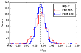
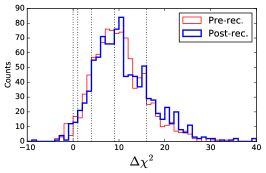
Figure 10: The distribution of best-fit values for $\alpha_{\rm iso}$ (left), estimated errors (center), and the $\Delta\chi^{2}$ (right panel) for the set of 1000 mock catalogs. Results before reconstruction are presented in red while results after reconstruction (method C) are presented in blue. Dashed lines on left panels indicate the expected value given cosmological model in Table 1. Dotted lines in the right panel indicates $\Delta\chi^{2}=\{0,1.0,4.0,9.0,16.0\}$, corresponding to BAO detection significances of 0, 1, 2, 3 and 4$\sigma$, respectively.

For the isotropic fits, values of $\alpha_{\rm iso}$ are consistent with the input within the 2$\sigma$ level for pre-reconstructed mocks and for two of the reconstruction methods (B and C). The rms of $\alpha_{\rm iso}$ values for pre-reconstructed mocks are larger than the average per-mock estimated error due to outliers of $\alpha_{\rm iso}$. For the post-reconstruction mocks, the rms and mean error are in good agreement. The average gain in estimated errors caused by reconstruction is $\sim 20$% and is clearly visible in Fig. 10. The significance of BAO detections are estimated in individual mocks by comparing the $\chi^{2}$ of a model with peak to the $\chi^{2}_{\rm no~{}peak}$ of a model without peak: $\Delta\chi^{2}=\chi^{2}_{\rm no~{}peak}-\chi^{2}$. Pre-reconstruction mocks show $\langle\Delta\chi^{2}\rangle=10.5$ corresponding to $\sim 3.2\sigma$ detection. Reconstruction slightly increases the significance by 0.2 to 1.6 unit in $\Delta\chi^{2}$, depending on the reconstruction procedure, reaching 3.5$\sigma$ for case C. Less than 4% of mocks produce no BAO detection, where $\Delta\chi^{2}<1$, even after reconstruction is applied.

Anisotropic fits on mock catalogs have similar behavior to the isotropic ones. Figure 11 reveals slightly more Gaussian distributions of $\alpha_{\perp}$ and $\alpha_{\parallel}$ after applying reconstruction. However, the mean values of $\alpha$ show a small bias relative to the expected input values. These biases represent 20% of the expected error of a single realization for pre-reconstruction mocks and they are reduced to 5-15% in post-reconstruction cases. These biases are caused mostly by the low statistical power of the current LRG sample which makes the $\alpha$ distributions non-Gaussian. If we fit the average correlation function of 1000 mock catalogs we are able to recover the input values within error bars. The average $\Delta\chi^{2}$ is virtually the same as the isotropic fits for both pre and post-reconstruction cases. Since we have two BAO parameters instead of one, the corresponding significance post-reconstruction is $\sim 3\sigma$. If mock catalogs are a good representation of real data, we expect a $\sim$4.8% measurement on $\alpha_{\perp}$ and $\sim 8.5$% on $\alpha_{\parallel}$ post-reconstruction.

Table 4: Results of anisotropic fits on the full set of 1000 reconstructed mock catalogs. Given the cosmological parameters in Table 1, the input values are: ${\alpha_{\perp}}_{0}=0.9791$ and ${\alpha_{\parallel}}_{0}=0.9880$. All fits are using $\Delta r=5$$h^{-1}$ Mpc bins. The column $N_{good}$ shows the number of mocks where $\Delta\chi^{2}>2.3$ from which all numbers are computed.

case	$N_{good}$	$\langle\alpha_{\perp}-{\alpha_{\perp}}_{0}\rangle$	rms$(\alpha_{\perp})$	$\langle\sigma_{\alpha_{\perp}}\rangle$	$\langle\alpha_{\parallel}-{\alpha_{\parallel}}_{0}\rangle$	rms$(\alpha_{\parallel})$	$\langle\sigma_{\alpha_{\parallel}}\rangle$	$\langle\chi^{2}_{r}\rangle$	$\langle\Delta\chi^{2}\rangle$
Pre-rec	926	$0.0120\pm 0.0021$	0.063	0.057	$-0.0192\pm 0.0037$	0.113	0.101	0.96	10.7
Post-rec (A)	938	$0.0078\pm 0.0016$	0.048	0.047	$0.0090\pm 0.0027$	0.084	0.071	0.98	12.1
Post-rec (B)	938	$0.0030\pm 0.0016$	0.050	0.048	$-0.0011\pm 0.0029$	0.089	0.088	0.97	11.9
Post-rec (C)	951	$0.0072\pm 0.0014$	0.044	0.044	$-0.0118\pm 0.0026$	0.080	0.062	0.96	12.9

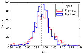
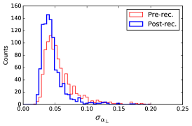
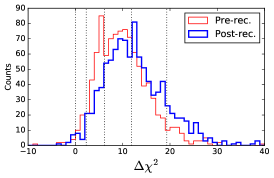
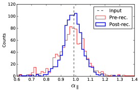
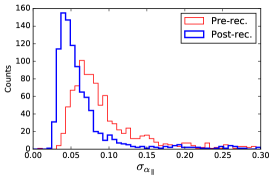
Figure 11: Same format as Fig. 10 but for $\alpha_{\perp}$ and $\alpha_{\parallel}$. Dotted lines in the right panel indicate $\Delta\chi^{2}=\{0,2.30,6.18,11.83,19.33\}$, corresponding to BAO detection significances of 0, 1, 2, 3 and 4$\sigma$, respectively. The reduction of the width of the $\alpha$ histograms is also seen as a global reduction of $\sigma_{\alpha}$ in the middle panels.

5 Results

In this section, we present our measurements, and the basic tests performed on the robustness of those measurements.

5.1 Fits to the Data

We performed BAO fits on the final eBOSS+CMASS NGC+SGC sample (unless otherwise stated), using the covariance matrix derived from mock catalogs. We scale our covariance matrices by a factor of 0.9753 to account for the slight mismatch in footprint area between data and mocks. In order to test the robustness of our measurements, fits were performed with a set of different choices for binning, $\Delta r$, and separation ranges, $r_{\rm min}<r<r_{\rm max}$. Our fiducial reconstruction method is method C (see section 4.3).

Table 5 presents the results for isotropic fits pre and post-reconstruction. All $\alpha_{\rm iso}$ values are stable and differ by less than 1$\sigma$. Estimated errors are also stable and no trend is seen when varying the choice of binning and fitting range. The average significance for BAO detection in this sample is $\sim 1.5\sigma$ for pre-reconstruction, increasing to $\sim 2.7\sigma$ after reconstruction. The estimated error on $\alpha_{\rm iso}$ is reduced by $\sim 40$% on average and $\chi^{2}$ values become closer to the number of degrees of freedom after reconstruction. The observed reduction in errors represents a significant improvement when compared to mock catalogs. Fig. 12 compares $\sigma_{\alpha_{\rm iso}}$ obtained pre and post-reconstruction for mocks and data. While the data appear to be at the extremes of the distribution, the error post-reconstruction is typical of that found in mocks.

Table 5: Isotropic fits on data for different choices of binning. In bold are the results for our fiducial analysis.

case				pre-reconstruction			post-reconstruction
Sample	$\Delta r$	$r_{\rm min}$	$r_{\rm max}$	$\alpha_{\rm iso}$	$\chi^{2}/$dof	$\Delta\chi^{2}$	$\alpha_{\rm iso}$	$\chi^{2}/$dof	$\Delta\chi^{2}$
NGC+SGC	5	32	182	$\bf{0.949^{+0.054}_{-0.051}}$	28.6/25	2.1	$\bf{0.968^{+0.026}_{-0.025}}$	18.9/25	7.8
		29	179	$0.928^{+0.049}_{-0.040}$	45.4/25	3.0	$0.975^{+0.029}_{-0.027}$	26.8/25	6.8
		30	180	$0.951^{+0.048}_{-0.049}$	51.5/25	1.8	$0.978^{+0.025}_{-0.022}$	30.0/25	8.7
		31	181	$0.949^{+0.045}_{-0.040}$	33.8/25	3.1	$0.966^{+0.026}_{-0.026}$	19.8/25	6.8
		28	178	$0.935^{+0.051}_{-0.045}$	33.0/25	2.6	$0.966^{+0.027}_{-0.023}$	27.2/25	8.8
	8	26	178	$0.961^{+0.048}_{-0.047}$	17.2/13	2.2	$0.974^{+0.024}_{-0.024}$	13.9/13	8.3
		28	180	$0.941^{+0.057}_{-0.045}$	9.5/14	2.3	$0.958^{+0.029}_{-0.026}$	7.2/14	7.1
		30	182	$0.932^{+0.055}_{-0.047}$	15.3/14	2.4	$0.968^{+0.025}_{-0.024}$	8.5/14	7.5
		32	184	$0.948^{+0.047}_{-0.046}$	17.2/13	2.9	$0.987^{+0.028}_{-0.026}$	14.3/13	6.5
NGC	5	30	180	$0.996^{+0.467}_{-0.079}$	49.4/25	0.0	$0.987^{+0.032}_{-0.031}$	32.8/25	6.2
SGC	5	30	180	$0.942^{+0.051}_{-0.049}$	59.5/25	2.3	$0.953^{+0.047}_{-0.052}$	23.2/25	1.9

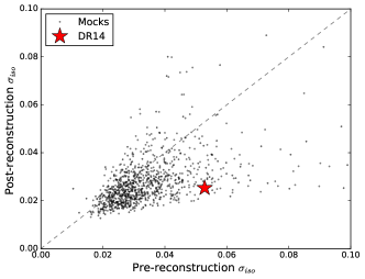
Figure 12: Estimated errors for the 1000 mocks. Pre-reconstruction results are shown in the x-axis and the post-reconstruction results (method C) are plotted on the y-axis. The red star indicates the result with our data sample. While the error pre-reconstruction with data is quite large compared to mocks, the error post-reconstruction is typical of those found in mocks.

Given the scatter in the significance of the measurement depending on the choice of analysis, we define our fiducial analysis as the one producing the $\Delta\chi^{2}$ that is the closest to the average values of all cases in Table 5, i.e., $\Delta r~{}=~{}5$ $h^{-1}$ Mpc and $(r_{\rm min},r_{\rm max})=(32,182)$ $h^{-1}$ Mpc. We also adopt this choice of fiducial analysis in our anisotropic fits below.

Fig. 13 shows the monopole and the two best-fit models (with and without BAO peak) on the reconstructed sample for our fiducial choice of analysis. Fig. 14 presents the $\chi^{2}$ values as a function of $\alpha_{\rm iso}$ and marginalizing over all other parameters for both models. The model without peak has a $\chi_{\rm no\ peak}^{2}$ about 7.8 units above the minimum of the model with peak, corresponding to a preference for the BAO peak model with a significance of 2.8$\sigma$.

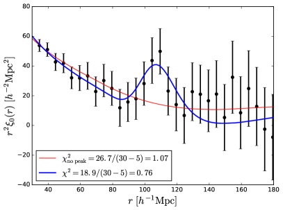
Figure 13: Monopole of the post-reconstruction correlation function with the best-fit models with a BAO peak component (blue thick line) and without peak (red thin line) for our fiducial choice of binning ($\Delta r=5$$h^{-1}$ Mpc and $32<r<182$$h^{-1}$ Mpc).

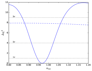
Figure 14: $\chi^{2}$ as a function of the dilation parameter $\alpha_{\rm iso}$ for both models (solid: with peak, dashed: without peak). This curve corresponds to our fiducial choice of analysis ($\Delta s=5$$h^{-1}$ Mpc and $32<r<182$$h^{-1}$ Mpc). The $\Delta\chi^{2}=7.8$ corresponds to a detection of 2.8$\sigma$ of the BAO peak.

Anisotropic fits are listed in Table 6 for the same analysis cases presented with isotropic fits. Best-fit $\alpha_{\perp}$ and $\alpha_{\parallel}$ values are mostly stable to changes in the analysis. However, errors on the pre-reconstruction sample are quite unstable due to the low significance of the measurement ($\Delta\chi^{2}\sim 3$ in average). Reconstruction stabilizes errors and increases the significance of our constraints ($\Delta\chi^{2}\sim 8$ in average). The estimated errors post-reconstruction are similar to average values found in mock catalogs (c.f. Table 4).

The left panel of Fig. 15 displays the best-fit anisotropic models compared to the data for our fiducial choice of analysis. The right panel shows the two dimensional $\chi^{2}$ contours for 1, 2 and 3$\sigma$, after converting $\alpha_{\perp}$ and $\alpha_{\parallel}$ into $D_{M}/r_{d}$ and $D_{H}/r_{d}$ respectively, using values of our fiducial cosmological model on Eq. 14. The likelihood becomes highly non-Gaussian beyond the $\Delta\chi^{2}=2.3$ contour due to the low statistical power of this sample. We expect that these contours will become more Gaussian as we increase the size our data sample in the future.

Table 6: Anisotropic fits on data for different binning choices. In bold are the results for our fiducial analysis (see text). Given the low statistical power of this sample for anisotropic fits, we do not include separate results for NGC or SGC.

case			pre-reconstruction					post-reconstruction
$\Delta r$	$r_{\rm min}$	$r_{\rm max}$	$\alpha_{\perp}$	$\alpha_{\parallel}$	$\chi^{2}/$dof	$\Delta\chi^{2}$	corr.	$\alpha_{\perp}$	$\alpha_{\parallel}$	$\chi^{2}/$dof	$\Delta\chi^{2}$	corr.
5	32	182	$\bf 0.99^{+0.08}_{-0.05}$	$\bf 0.82^{+0.09}_{-0.08}$	75.2/50	1.5	-0.40	$\bf 1.01^{+0.04}_{-0.03}$	$\bf 0.88^{+0.06}_{-0.17}$	66.5/50	7.2	-0.35
	28	178	$1.00^{+0.11}_{-0.06}$	$0.83^{+0.07}_{-0.07}$	66.0/50	2.8	-0.44	$1.01^{+0.04}_{-0.04}$	$0.84^{+0.06}_{-0.06}$	63.7/50	10.1	-0.13
	29	179	$1.00^{+0.07}_{-0.05}$	$0.83^{+0.06}_{-0.07}$	75.6/50	4.7	-0.48	$1.02^{+0.05}_{-0.04}$	$0.83^{+0.08}_{-0.06}$	54.5/50	8.1	-0.80
	30	180	$1.01^{+0.08}_{-0.05}$	$0.82^{+0.08}_{-0.08}$	89.7/50	3.0	-0.68	$1.02^{+0.04}_{-0.04}$	$0.85^{+0.12}_{-0.12}$	62.4/50	7.8	-0.86
	31	181	$1.00^{+0.06}_{-0.05}$	$0.83^{+0.08}_{-0.08}$	75.3/50	3.5	-0.35	$1.00^{+0.04}_{-0.04}$	$0.92^{+0.06}_{-0.27}$	62.7/50	5.5	-0.69

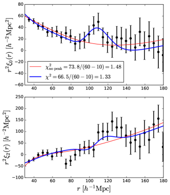
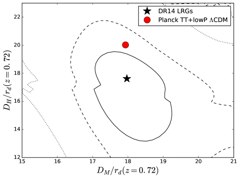
Figure 15: Left panel: monopole (top) and quadrupole (bottom) of the post-reconstruction correlation function with the best-fit models with (blue thick line) and without (red thin line) a BAO peak component. Right panel: $\chi^{2}$ contours as a function of the dilation parameters $\alpha_{\perp},\alpha_{\parallel}$ converted to $D_{M}/r_{d}$ and $D_{H}/r_{d}$ using our fiducial cosmology in Table 1. The contours correspond to $\chi^{2}-\chi^{2}_{\rm min}=2.3,6.18,11.83$ (solid, dashed and dotted, respectively). For this fit, we obtain $\Delta\chi^{2}=7.2$.

5.2 Comparison with previous BAO measurements

We summarize current distance measurements using BAO in Figure 16. The distances are normalized to the predictions using a Planck cosmology. Our measurement of the isotropic BAO scale at $z=0.72$ is consistent with that of Planck at about the 1$\sigma$ level.

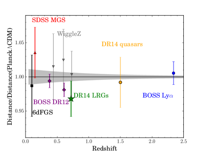
Figure 16: Current isotropic BAO measurements as a function of redshift compared to the prediction given by the best-fit cosmological parameters of Planck TT+TE+EE+lowP (Planck Collaboration XIII, 2016). Our measurement is indicated by the green star labeled “DR14 LRGs”. The other BAO measurements are: 6dFGRS at $z=0.11$ (Beutler et al., 2011), SDSS MGC at $z=0.15$ (Ross et al., 2015), BOSS DR12 at $z=[0.38,0.61]$ (Alam et al., 2017), WiggleZ at $z=[0.44,0.6,0.73]$ (Blake et al., 2011a), eBOSS DR14 QSO sample at $z=1.52$ (Ata el al., 2018), and BOSS DR12 Lyman-$\alpha$ sample at $z=2.3$ (Bautista et al., 2017; du Mas des Bourboux et al., 2017).

Given that our eBOSS LRG sample was combined with the high-redshift tail of the CMASS sample in overlapping areas, the BAO measurements at $0.50<z<0.75$ from CMASS and ours, at $0.6<z<1.0$, are correlated. This correlation can be estimated by assuming that the covariance is proportional to the effective overlap volume between the two surveys. Using the CMASS $\bar{n}(z)$ over the effective area of eBOSS (overlapping area) covering 1844 deg², and computing Eq. 5 over $0.6<z<0.75$ (overlapping redshift range), we obtain an effective overlap volume of $V_{\rm eff}[{\rm CMASS\cap eBOSS}]=0.31$ Gpc³. Therefore, we estimate the correlation coefficient between the two measurements to be

$$\rho=\frac{V_{\rm eff}({\rm CMASS\cap eBOSS})}{\sqrt{V_{\rm eff}({\rm CMASS})V_{\rm eff}({\rm eBOSS})}}=\frac{0.31}{\sqrt{4.1\times 0.9}}=0.16.$$ (19)

We leave more realistic calculations of this correlation using correlated mock catalogs (as in, e.g., Beutler et al. 2016) for future work.

Forecasts in Zhao et al. (2016) predict 1% precision on isotropic BAO with 7000 deg² for the final eBOSS LRG sample (when combined with the high-redshift tail of CMASS). For the current footprint with $A_{\rm eff}=1844$ deg² the forecast scales to a 1.95% BAO measurement assuming that error is proportional to square-root of the effective volume. Our isotropic BAO measurement with a 2.6% error is slightly larger than this forecast. This might be caused by holes in the footprint due to plates still not observed and to the various masks applied to our sample. These effects increase the size of boundaries of the survey and might increase errors relative to forecasts which consider uniform volumes. The larger error of our measurement compared to the forecast might also be due to statistical fluctuations, since the distribution of estimated errors has a large dispersion, as observed with mock catalogs in Fig. 10. Previous BAO measurements (e.g. Alam et al. 2017; Ata el al. 2018) typically also report estimated errors that are larger than predictions.

6 Conclusion

We present the first BAO measurement using luminous red galaxies from the first two years of data taken in the eBOSS survey. The total area observed, weighted by the fiber completenes, is 1844 deg², yielding an effective volume of 0.9 Gpc³ over $0.6<z<1.0$ when combining the eBOSS LRG sample with the CMASS $z>0.6$ galaxies over the eBOSS footprint. We obtain a 2.6% spherically averaged distance measurement after reconstruction at $z_{\rm eff}=0.72$ that is consistent at 1$\sigma$ level with the predictions of the $\Lambda$CDM model assuming a Planck best-fit cosmology.

In this analysis we introduce a novel technique to account for redshift failures, while also propagating photometric systematics to the random catalog. This technique yields unbiased measurements of the correlation function, as tested on mock catalogs, and will be essential for future analyses using the full-shape information such as redshift space distortion studies.

When eBOSS will have finished its observing program, we expect that 7000 deg² of area will have been observed spectroscopically, representing a reduction on errors of isotropic BAO measurements of a factor of $\sqrt{7000/1844}\sim 2$ (assuming errors scale with the square root of the area).

The new software used to produce catalogs, compute model for failures, fit BAO peak, and apply reconstruction are all implemented in Python and available at github.com/julianbautista/eboss_clustering.

Upcoming surveys will significantly improve upon our results; the DESI survey will observe LRG spectra with similar depths and redshift ranges than eBOSS. We expect that the framework presented here should be applicable for DESI clustering measurements using both LRGs and ELGs, where sub-percent errors on BAO are expected.

References

- Aihara et al. (2011) Aihara, H., Allende Prieto, C., An, D., et al. 2011, ApJS, 193, 29
- Alam et al. (2015a) Alam, S., Albareti, F. D., Allende Prieto, C., et al. 2015, ApJS, 219, 12
- Alam et al. (2017) Alam, S., Ata, M., Bailey, S., et al. 2017, astro-ph/1607.03155
- Albofathi et al. (2017) Albofathi, B., Aguado, D., Aguilar, G., et al. 2017, arXiv:1707.09322
- Anderson et al. (2012) Anderson, L., Aubourg, E., Bailey, S., et al. 2012, MNRAS, 427, 3435
- Anderson et al. (2014a) Anderson, L., Aubourg, E., Bailey, S., et al. 2014, MNRAS, 439, 83
- Anderson et al. (2014b) Anderson, L., Aubourg, E., Bailey, S., et al. 2014, MNRAS, 441, 24
- Ata el al. (2018) Ata, M., Baumgarten, F., Bautista, J., et al. 2018, MNRAS, 473, 4773
- Bautista et al. (2017) Bautista, J., Busca, N., Guy, J., Rich, J., et al. 2017, A&A, 603, A12
- Beutler et al. (2011) Beutler, F., Blake, C., Colless, M., et al. 2011, MNRAS, 416, 3017
- Beutler et al. (2014) Beutler, F., Shun, S., Brownstein, J., et al. 2014, MNRAS, 444, 3501
- Beutler et al. (2016) Beutler, F., Blake, C., Koda, J., et al. 2016, MNRAS, 455, 3230
- Beutler et al. (2017a) Beutler, F., Seo, H.-J., Ross, A., et al. 2017, MNRAS, 464, 3409
- Bianchi & Percival (2017) Bianchi D., Percival W.J., 2017, arXiv:1703.02070
- Blake et al. (2011a) Blake C., et al., 2011, MNRAS, 418, 1707
- Blanton et al. (2017) Blanton, M., Bershady, M., 2017, AJ, 154, 28
- Bolton et al. (2012) Bolton A., et al., 2012, AJ, 144, 144
- Bond & Efstathiou (1987) Bond, R., & Efstathiou, G., 1987, MNRAS, 226, 665
- Burden et al. (2014) Burden, A., Percival, W. J., Manera, M., 2014, MNRAS, 445, 3152
- Burden, Percival & Howlett (2015) Burden, A., Percival, W. J., Howlett, C., 2015, MNRAS, 453, 456
- Clifton et al. (2012) Clifton, T., Ferreira, P., Padilla, A., & Skordis, C., 2012, PhysRep, 513, 1
- Cole et al. (2005) Cole, S., Percival, W. J., Peacock, J. A., et al. 2005, MNRAS, 362, 505
- Cui et al. (2008) Cui, W., Liu, L, Yang, X., et al. 2008, ApJ, 687, 738
- Colless et al. (2003) Colless M., et al., 2003, astro-ph/0306581
- Cunha et al. (2017) Cunha, E., Hopkins, A., Colless, M., et al. 2017, astro-ph/1706.01246
- Dawson et al. (2013) Dawson K. S., et al., 2013, AJ, 145, 10
- Dawson et al. (2016) Dawson K. S., et al., 2016, AJ, 151, 44
- Delubac et al. (2017) Delubac, T., Raichoor, A., Comparat, J., et al. 2017, MNRAS, 465, 1831
- DESI collaboration (2016a) DESI Collaboration, 2016a, astro-ph/1611.00036
- DESI collaboration (2016b) DESI Collaboration, 2016b, astro-ph/1611.00037
- Doi et al. (2010) Doi, M., Tanaka, M., Fukugita, M., et al. 2010, AJ, 139, 1628
- Drinkwater et al. (2010) Drinkwater, M., Russell, J., Blake, C., et al. 2010, MNRAS, 401, 1429
- du Mas des Bourboux et al. (2017) du Mas des Bourboux, H., Le Goff, J. M., Blomqvist, M., et al. 2017, accepted A&A, astro-ph/1708.02225
- Eisenstein et al. (2005) Eisenstein, D. J., Zehavi, I., Hogg, D. W., et al. 2005, ApJ, 633, 560
- Eisenstein et al. (2007) Eisenstein, D. J., Seo, H.-J., Sirko, E., & Spergel, D. N. 2007, ApJ, 664, 675
- Eisenstein et al. (2011) Eisenstein D. J., et al., 2011, AJ, 142, 72
- Euclid Collaboration (2013) Amendola, L., Appleby, S., Bacon, D., 2013, LLR, 16, 6
- Feldman, Kaiser, & Peacock (1994) Feldman, H. A., Kaiser, N., Peacock, J. A. 1994, ApJ, 426, 23
- Font-Ribera et al. (2014) Font-Ribera, A., McDonald, P., Mostek, N., et al. 2014, JCAP, 05, 23
- Fukugita et al. (1996) Fukugita, M.; Ichikawa, T.; Gunn, J.; et al. 1996, AJ, 111, 1748
- Gil-Marín et al. (2017) Gil-Marín, H., Percival, W., Verde, L., et al. 2017, MNRAS, 465, 1757
- Gil-Marín et al. (in prep) Gil-Marín, H., Guy, J., Burtin, E., et al. in prep.
- Guo et al. (2012) Guo, H., Zehavi, I., Zheng, Z., ApJ, 756, 2
- Gunn et al. (2006) Gunn J.E., et al., 2006, AJ, 131, 2332
- Hartlap et al. (2007) Hartlap, J., Simon, P. & Schneider, P., 2007 A&A, 464, 399
- Ho et al. (2012) Ho, S., Cuesta, A., Seo, H.-J., et al. 2012, ApJ, 761, 14
- Høg et al. (2000) Høg, E., Fabricius, C., Makarov, V. V., et al. 2000, A&A, 355, 27
- Hutchinson et al. (2016) Hutchinson, T., Bolton, A., Dawson, K., AJ, 152, 205
- Jensen et al. (2016) Jensen, T., Vivek, M., Dawson, K., ApJ, 833, 199
- Jones et al. (2009) Jones, D. H., Read, M., Saunders, W., et al. 2009, MNRAS, 339, 683
- Kirkby et al. (2013) Kirkby D., et al., 2013, JCAP, 3, 24
- Landy & Szalay (1993) Landy, Stephen D., & Szalay, Alexander S., 1993, ApJ, 412, 64
- Lang et al. (2014) Lang, D., Hogg, D. W., & Schlegel, D. J. 2014, arXiv:1410.7397
- Laureijs et al. (2011) Laureijs R., et al., 2011, arXiv:1110.3193
- Lewis et al. (2000) Lewis, A., Challinor, A., & Lasenby, A., ApJ, 538, 473
- Myers et al. (2015) Myers, A., Palanque-Delabrouille, N., Prakash, A., et al. 2015, ApJS, 221, 27
- Peebles & Yu (1970) Peebles, P. & Yu, J., 1970, ApJ, 162, 815
- Percival et al. (2001) Percival W. J., 2001, MNRAS, 327, 1297
- Percival et al. (2007) Percival W.J., et al., 2007, MNRAS, 381, 1053
- Percival et al. (2014) Percival, W. J., Ross, A. J., Sánchez, A. G., et al. 2014, MNRAS, 439, 2531
- Planck Collaboration I (2016) Planck Collaboration I, Ade P.A.R., et al., 2016, A& A, 594, 1
- Planck Collaboration XIII (2016) Planck Collaboration XIII, Ade P.A.R., et al., 2016, A& A, 594, A13
- Prakash et al. (2015) Prakash, A., Licquia, T., Newman, J., et al. 2016, ApJ, 803, 2
- Prakash et al. (2016) Prakash, A., Licquia, T., Newman, J., et al. 2016, ApJS, 224, 34
- Raichoor et al. (2017) Raichoor, A., Comparat, J., Delubac, T., et al. 2017, MNRAS, 471, 3955
- Reid et al. (2016) Reid, B., Ho, S., Padmanabhan, N., et al. 2016, MNRAS, 455, 1553
- Rykoff et al. (2014) Rykoff, E. S., Rozo, E., Busha, M. T., et al. 2014, ApJ, 785, 104
- Ross et al. (2011) Ross, A., Ho, S., Cuesta, A., et al. 2011, MNRAS, 417, 1350
- Ross et al. (2012) Ross, A., Percival, W., Sánchez, A., et al. 2012, MNRAS, 424, 564
- Ross et al. (2015) Ross, A. J., Samushia, L., Howlett, C., et al. 2015, MNRAS, 449, 835
- Ross et al. (2017) Ross, A., Beutler, F., Chuang, C.-H., et al. 2017, MNRAS, 464, 1668
- SDSS Collaboration (2016) SDSS Collaboration, 2016, arXiv:1608.02013
- Seo et al. (2016) Seo, H-J., Beutler, F., Ross, A., & Saito, S., 2016, MNRAS, 460, 2453
- Smee et al. (2013) Smee S., et al., 2013, AJ, 146, 32
- Sunyaev & Zeldovich (1970) Sunyaev, R., & Zeldovich, Y., 1970, Ap&SS, 7, 3
- Taylor et al. (2014) Taylor, A., Joachimi, B. & Kitching, T., 2014, MNRAS, 432, 1928
- Tojeiro et al. (2014) Tojeiro, R., Ross, A. J., Burden, A., et al. 2014, MNRAS, 440, 2222
- Vargas-Magaña et al. (2017) Vargas-Magaña, M., Ho, S., Fromenteau, S., et al. 2017, MNRAS, 467, 2331
- Weinberg et al. (2013) Weinberg, D., Mortonson, M., Eisenstein, D., et al. 2013, PhysRep, 530, 87
- White et al. (2014) White, M., Tinker, J. L., & McBride, C. K. 2014, MNRAS, 437, 2594
- White (2015) White, M., 2015, MNRAS, 450, 3822
- Wright et al. (2010) Wright, E., Eisenhardt, P., Mainzer, A., 2010, 140, 1868
- York et al. (2000) York, D.G., et al., 2000, AJ, 120, 1579
- Zarrouk et al. (in prep) Zarrouk, P., Burtin, E., et al. in prep.
- Zhai et al. (2017) Zhai, Z., Tinker, J., Hahn, C., et al. 2017, ApJ, 848, 76
- Zhao et al. (2016) Zhao, G., Wang, Y., Ross, A., et al. 2016, MNRAS, 457, 2377