Abstract

We consider in this paper a microscopic model (that is, a system of three reaction-diffusion equations) incorporating the dynamics of handling and searching predators, and show that its solutions converge when a small parameter tends to $0$ towards the solutions of a reaction-cross diffusion system of predator-prey type involving a Holling-type II or Beddington-DeAngelis functional response. We also provide a study of the Turing instability domain of the obtained equations and (in the case of the Beddington-DeAngelis functional response) compare it to the same instability domain when the cross diffusion is replaced by a standard diffusion.

Keywords: Cross diffusion equations, predator-prey equations, Turing instability, Turing patterns, functional responses

AMS Classification: 35B25, 35B36, 35K45, 35K57, 35Q92, 92D25

1 Introduction

1.1 General presentation

Complex functional responses are widely used in predator-prey models [1, 2, 3, 4, 5]. For example, the Holling-type II functional response [1] is based on the idea that predators will catch a limited proportion of available prey in the case when preys are abundant. Denoting with $N:=N(t)$ the prey biomass, and with $P:=P(t)$ the predator biomass, this type of functional response leads to the following set of two ODEs:

$$\begin{split}\dot{N}&=r_{0}g(N)-\dfrac{bNP}{1+kN},\\ \dot{P}&=\dfrac{cbNP}{1+kN}-\mu P,\end{split}$$ (1)

where $r_{0},\;b,\;c,\;k,\;\mu>0$, and where the function $g$ describes the prey growth and can be either linear, that is $g(N)=N$, or involve a logistic part as $g(N)=(1-\eta N)N$ with $\eta>0$ [6]. Note that when $g(N)=N$ and $k=0$, one recovers the classical Lotka-Volterra predator-prey model.

If one also wishes to take into account the competition between predators when they try to catch prey, the slightly more complex Beddington-DeAngelis functional response can be introduced [3, 4]:

$$\begin{split}\dot{N}&=r_{0}g(N)-\dfrac{bNP}{1+kN+hP},\\ \dot{P}&=\dfrac{cbNP}{1+kN+hP}-\mu P,\end{split}$$ (2)

where $r_{0},\;b,\;c,\;k,\;h>0$.

An important point in the sequel will be the observation that predator-prey models with the Beddington-DeAngelis functional response are known to produce patterns (coming out of a Turing instability) when diffusion terms with suitable rates (denotes by $d_{N},\;d_{P}$) are added to the reaction term [7, 8]. In such a situation, the system becomes:

$$\begin{split}\partial_{t}N-d_{N}\Delta_{x}N&=r_{0}g(N)-\dfrac{bNP}{1+kN+hP},\\ \partial_{t}P-d_{P}\Delta_{x}P&=\dfrac{cbNP}{1+kN+hP}-\mu P.\end{split}$$ (3)

On the other hand, no patterns are known to appear in the case of a reaction-diffusion predator-prey model with a Holling-type II functional response and diffusion terms as in (3) [9] (patterns may however appear when richer dynamics are considered, for example when one adds quadratic intra-predator interaction or fighting term [10, 11], or a density-dependent predator mortality [11]). In all these cases, a fundamental assumption is that the diffusion coefficients of the two species must be different; patterns appearing taking equal diffusion coefficient are studied in [12, 13, 14]).

Several works were written in the past in order to obtain a derivation of the Holling-type II and Beddington-DeAngelis functional responses out of simple and realistic “microscopic models” which in some limit lead, at least formally, to (1) or (2). Such a model was designed by Metz and Diekmann [15] for the Holling-type II functional response, and by Geritz and Gyllenberg [16], Huisman and De Boer [17], for the Beddington-DeAngelis one, and references therein.

Metz and Diekmann proposed a system of three ODEs, in which the predators are divided in two classes (respectively called searching and handling), while the interaction between predators and preys is treated in a quite simple way (standard Lotka-Volterra terms are used). Predators which are searching for preys become handling with a rate proportional to the number of preys and come back to the searching state with a constant rate. Only handling predators contribute to the reproduction (and give birth to a searching predator), while the mortality rate (in absence of prey) is constant and equal for the two classes. The searching-handling switch is supposed to happen on a much faster time scale than the reproduction and mortality processes. The corresponding parameter in the system of ODEs is therefore called $1/\varepsilon$, and the system writes (for some $r_{0}$, $\alpha$, $\tilde{\gamma}$, $\Gamma$, $\mu$, $\varepsilon>0$)

$$\begin{split}\dot{N}^{\varepsilon}&=r_{0}N^{\varepsilon}-\alpha N^{\varepsilon}p_{s}^{\varepsilon},\\ \dot{p}_{s}^{\varepsilon}&=\dfrac{1}{\varepsilon}\left(-\alpha N^{\varepsilon}p_{s}^{\varepsilon}+\tilde{\gamma}p_{h}^{\varepsilon}\right)+\Gamma p_{h}^{\varepsilon}-\mu p_{s}^{\varepsilon},\\ \dot{p}_{h}^{\varepsilon}&=\dfrac{1}{\varepsilon}\left(\alpha N^{\varepsilon}p_{s}^{\varepsilon}-\tilde{\gamma}p_{h}^{\varepsilon}\right)-\mu p_{h}^{\varepsilon},\end{split}$$ (4)

where $N^{\varepsilon}$ still is the density of preys, while $p_{h}^{\varepsilon}$ and $p_{s}^{\varepsilon}$ are the respective densities of handling and searching predators. It is shown that in the formal limit $\varepsilon\to 0$, one gets $N^{\varepsilon}\to N$ and $p_{s}^{\varepsilon}+p_{h}^{\varepsilon}\to P$ where $N,\;P$ satisfy (1) (with $g(N):=N$, $b:=\alpha,\;k:=\alpha/\tilde{\gamma},\;c:=\Gamma/\tilde{\gamma}$) [15].

A similar procedure was later applied by Geritz and Gyllenberg in a more complex situation [16]: they divided not only the predator population into searchers and handlers, but also structured the prey population into two classes, the class of active preys (typically foraging) and prone to predation, and the class of those prey individuals who have found a refuge and cannot be caught by predators. In this way, they derived the Beddington-DeAngelis functional response in terms of mechanisms at the individual level avoiding the usual interference between predators. Previously, Huisman and De Boer [17], starting from a different four-dimensional model also obtained a system of two ordinary differential equations (they however simplified a complicated quadratic expression with a Padé approximation to recover the standard formula of the Beddington-DeAngelis functional response). In both cases, two different time scales were exploited.

We are interested in this paper in the introduction of diffusion processes in the asymptotic problem (4). Denoting by $d_{1},\;d_{2},\;d_{3}>0$ the diffusion rates of preys, searching predators and handling predators respectively, one can write, keeping the reaction term of (4), the following reaction-diffusion system:

$$\begin{split}\partial_{t}N^{\varepsilon}-d_{1}\Delta_{x}N^{\varepsilon}&=r_{0}\left(1-\eta N^{\varepsilon}\right)N^{\varepsilon}-\alpha N^{\varepsilon}p_{s}^{\varepsilon},\\ \partial_{t}p_{s}^{\varepsilon}-d_{2}\Delta_{x}p_{s}^{\varepsilon}&=\dfrac{1}{\varepsilon}\left(-\alpha N^{\varepsilon}p_{s}^{\varepsilon}+\tilde{\gamma}\,p_{h}^{\varepsilon}\right)+\Gamma p_{h}^{\varepsilon}-\mu p_{s}^{\varepsilon},\\ \partial_{t}p_{h}^{\varepsilon}-d_{3}\Delta_{x}p_{h}^{\varepsilon}&=\dfrac{1}{\varepsilon}\left(\alpha N^{\varepsilon}p_{s}^{\varepsilon}-\tilde{\gamma}\,p_{h}^{\varepsilon}\right)-\mu p_{h}^{\varepsilon}.\end{split}$$ (5)

Note that we systematically expect the diffusion rate $d_{3}$ of handling predators to be smaller than the diffusion rate of searching predators $d_{2}$. The formal limit of this system when $\varepsilon\to 0$ is the set of two reaction cross-diffusion equations:

$$\begin{split}\partial_{t}&N-d_{1}\Delta_{x}N=r_{0}(1-\eta N)N-\frac{\tilde{\gamma}\alpha N}{\alpha N+\tilde{\gamma}}P,\\ \partial_{t}&P-\Delta_{x}\bigg{(}\frac{d_{2}\tilde{\gamma}+d_{3}\alpha N}{\alpha N+\tilde{\gamma}}\,P\bigg{)}=\Gamma\frac{\alpha N\,P}{\alpha N+\tilde{\gamma}}-\mu P,\end{split}$$ (6)

in which the reaction terms are identical (up to the change of name of the constant parameters) to those of (1), but in which the diffusion term relative to predators is much more complicated than a constant times Laplacian of $P$ (terms like $d\Delta_{x}P$ will be systematically called linear diffusive terms in the sequel, while cross diffusion refers to terms like $\Delta_{x}(f(N,P)\,P)$, where $f$ is a smooth non-constant function of $N,\>P$, as in the second equation of (6)). It can be noticed that the resulting cross-diffusion term is a convex combination of the diffusion coefficients $d_{2}$ and $d_{3}$ of the microscopic system. In Subsection 1.2 of the Introduction of this paper, we state a rigorous theorem showing that convergence of solutions to system (5) towards solutions to system (6) indeed holds when suitable functional spaces are introduced.

The same procedure can be applied in the case of Beddington-DeAngelis like functional response, that is a system of ODEs close to (2). First, we introduce a system of three ordinary differential equations modeling the interaction between preys, handling and searching predators as in (5), but in which we also take into account the competition among predators when they look for preys. This is done thanks to the introduction of the denominator $1+\xi p_{s}$, for some $\xi>0$, in the interaction term between predators and preys. The system writes as follows:

$$\begin{split}\dot{N}^{\varepsilon}&=r_{0}(1-\eta N^{\varepsilon})N^{\varepsilon}-\dfrac{\alpha N^{\varepsilon}p_{s}^{\varepsilon}}{1+\xi p_{s}^{\varepsilon}},\\ \dot{p}_{s}^{\varepsilon}&=\dfrac{1}{\varepsilon}\left(-\dfrac{\alpha N^{\varepsilon}p_{s}^{\varepsilon}}{1+\xi p_{s}^{\varepsilon}}+\tilde{\gamma}p_{h}^{\varepsilon}\right)+\Gamma p_{h}^{\varepsilon}-\mu p_{s}^{\varepsilon},\\ \dot{p}_{h}^{\varepsilon}&=\dfrac{1}{\varepsilon}\left(\dfrac{\alpha N^{\varepsilon}p_{s}^{\varepsilon}}{1+\xi p_{s}^{\varepsilon}}-\tilde{\gamma}p_{h}^{\varepsilon}\right)-\mu p_{h}^{\varepsilon}.\end{split}$$ (7)

Its formal limit when $\varepsilon\to 0$ is then a system close to (2), also obtained in [17] starting from a system of four ODEs in which all interactions are linear/quadratic.

A reaction-diffusion system corresponding to (7), where the diffusion of preys, searching predators, and handling predators is taken into account through diffusion rates $d_{1},\;d_{2},\;d_{3}>0$, writes:

$$\begin{split}\partial_{t}N^{\varepsilon}-d_{1}\Delta_{x}N^{\varepsilon}&=r_{0}\left(1-\eta N^{\varepsilon}\right)N^{\varepsilon}-\dfrac{\alpha N^{\varepsilon}p_{s}^{\varepsilon}}{1+\xi p_{s}^{\varepsilon}},\\ \partial_{t}p_{s}^{\varepsilon}-d_{2}\Delta_{x}p_{s}^{\varepsilon}&=\dfrac{1}{\varepsilon}\bigg{(}-\frac{\alpha N^{\varepsilon}p_{s}^{\varepsilon}}{1+\xi p_{s}^{\varepsilon}}+\tilde{\gamma}p_{h}^{\varepsilon}\bigg{)}+\Gamma p_{h}^{\varepsilon}-\mu p_{s}^{\varepsilon},\\ \partial_{t}p_{h}^{\varepsilon}-d_{3}\Delta_{x}p_{h}^{\varepsilon}&=-\frac{1}{\varepsilon}\bigg{(}-\frac{\alpha N^{\varepsilon}p_{s}^{\varepsilon}}{1+\xi p_{s}^{\varepsilon}}+\tilde{\gamma}p_{h}^{\varepsilon}\bigg{)}-\mu p_{h}^{\varepsilon}.\end{split}$$ (8)

We present in Subsection 1.2 of the Introduction a rigorous result of convergence of the solutions to this system towards the solution of a reaction-cross diffusion system where the reaction part is close to (2). This system writes

$$\begin{split}\dfrac{\partial N}{\partial T}&-d_{1}\Delta_{x}N=r\left(1-\eta\,N\right)N-\dfrac{2\alpha\tilde{\gamma}NP}{\tilde{\gamma}+\alpha N+\tilde{\gamma}\xi P+\sqrt{(\tilde{\gamma}+\alpha N-\tilde{\gamma}\xi P)^{2}+4\tilde{\gamma}2\,\xi P}},\\ \dfrac{\partial P}{\partial T}&-\Delta_{x}\left(f(N,P)P\right)=\dfrac{2\alpha\Gamma NP}{\tilde{\gamma}+\alpha N+\tilde{\gamma}\xi P+\sqrt{(\tilde{\gamma}+\alpha N-\tilde{\gamma}\xi P)^{2}+4\tilde{\gamma}2\,\xi P}}-\mu P,\end{split}$$ (9)

where

$$f(N,P)=d_{2}\dfrac{2\tilde{\gamma}}{\tilde{\gamma}+\alpha N-\tilde{\gamma}\xi P+\sqrt{(\tilde{\gamma}+\alpha N-\tilde{\gamma}\xi P)^{2}+4\tilde{\gamma}2\,\xi P}}\\ +d_{3}\dfrac{2\alpha N}{\tilde{\gamma}+\alpha N+\tilde{\gamma}\xi P+\sqrt{(\tilde{\gamma}+\alpha N-\tilde{\gamma}\xi P)^{2}+4\tilde{\gamma}2\,\xi P}}.$$ (10)

The proof of this result as well as the proof of the theorem corresponding to the Holling-type II functional response, is based on estimates coming out of two classes of methods. On one hand, we use the duality lemmas devised for reaction-diffusion systems by M. Pierre and D. Schmitt [18]. More precisely, we use an improved version of those lemmas allowing to recover $L^{p}$ bounds for $p>2$ for the solutions of such systems [19, 20]. On the other hand, we also use entropy-like functionals which are strongly reminiscent of those used in works in which microscopic models for the Shigesada-Kawasaki-Teramoto system [21] are studied [22].

These proofs can also be compared to recent results in which reaction-cross diffusion systems are obtained as limits of standard reaction-diffusion systems with more equations, in the context of chemistry or biology [23, 24, 25, 26, 27, 28, 29, 30, 31].

As already mentioned, the Beddington-DeAngelis like functional response is particularly interesting since it is known that predator-dependent functional responses can lead to patterns when (linear) diffusion terms are added to the reaction terms, like for example in the following system (with reaction terms identical to those in (9)):

$$\begin{split}\dfrac{\partial N}{\partial T}&-D_{1}\Delta_{x}N=r\left(1-\eta\,N\right)N-\dfrac{2\alpha\tilde{\gamma}NP}{\tilde{\gamma}+\alpha N+\tilde{\gamma}\xi P+\sqrt{(\tilde{\gamma}+\alpha N-\tilde{\gamma}\xi P)^{2}+4\tilde{\gamma}2\,\xi P}},\\ \dfrac{\partial P}{\partial T}&-D\Delta_{x}P=\dfrac{2\alpha\Gamma NP}{\tilde{\gamma}+\alpha N+\tilde{\gamma}\xi P+\sqrt{(\tilde{\gamma}+\alpha N-\tilde{\gamma}\xi P)^{2}+4\tilde{\gamma}2\,\xi P}}-\mu P,\end{split}$$ (11)

However, if one consider that the Beddington-DeAngelis like functional response is coming out of an asymptotics when $\varepsilon\to 0$ of (8), one should rather study the possible appearance of patterns starting from system (9). We will describe the study that we performed concerning this issue in Subsection 1.3 of the Introduction. Note that for Holling-type II functional response, no patterns appear when the cross diffusion model (6) is considered, at least under the (biologically reasonable) assumption $d_{3}<d_{2}$, so that the qualitative behavior of (3) and (6) is not expected to be different.

1.2 Rigorous results of convergence

We consider in this subsection the system (8) in a smooth bounded open subset $\Omega$ of $\mathbb{R}^{d}$:

$$\partial_{t}N^{\varepsilon}-d_{1}\Delta_{x}N^{\varepsilon} =r_{0}\left(1-\eta N^{\varepsilon}\right)N^{\varepsilon}-\dfrac{\alpha N^{\varepsilon}p_{s}^{\varepsilon}}{1+\xi p_{s}^{\varepsilon}},$$ (12)

$$\partial_{t}p_{s}^{\varepsilon}-d_{2}\Delta_{x}p_{s}^{\varepsilon} =\dfrac{1}{\varepsilon}\bigg{(}-\frac{\alpha N^{\varepsilon}p_{s}^{\varepsilon}}{1+\xi p_{s}^{\varepsilon}}+\tilde{\gamma}p_{h}^{\varepsilon}\bigg{)}+\Gamma p_{h}^{\varepsilon}-\mu p_{s}^{\varepsilon},$$ (13)

$$\partial_{t}p_{h}^{\varepsilon}-d_{3}\Delta_{x}p_{h}^{\varepsilon} =-\frac{1}{\varepsilon}\bigg{(}-\frac{\alpha N^{\varepsilon}p_{s}^{\varepsilon}}{1+\xi p_{s}^{\varepsilon}}+\tilde{\gamma}p_{h}^{\varepsilon}\bigg{)}-\mu p_{h}^{\varepsilon},$$ (14)

together with homogeneous Neumann boundary conditions ($\hat{n}(x)$ denoting the exterior normal to $\Omega$ at a point $x\in\partial\Omega$)

$$\forall x\in\partial\Omega,\qquad\hat{n}(x)\cdot\nabla_{x}N^{\varepsilon}=0,\quad\hat{n}(x)\cdot\nabla_{x}p_{s}^{\varepsilon}=0,\quad\hat{n}(x)\cdot\nabla_{x}p_{h}^{\varepsilon}=0.$$ (15)

All parameters $r_{0}$, $\alpha$, $\tilde{\gamma}$, $\Gamma$, $\mu$, $d_{i}$ in this system are strictly positive, except $\eta$ and $\xi$, which are supposed to be nonnegative. When $\eta=0$, no direct logistic saturation is imposed on the preys, while when $\xi=0$, no competition between predators is assumed. Note that when both $\eta$ and $\xi$ are equal to zero, the reaction part of the system (12)-(14) reduces to (4).

We begin with a rigorous result for the passage to the limit $\varepsilon\to 0$ in the case $\xi=0$:

Theorem 1.1.

Let $\Omega$ be a smooth bounded open subset of $\mathbb{R}^{d}$ (for some dimension $d\in\mathbb{N}-\{0\}$), $d_{1},d_{2},d_{3}>0$ be diffusion rates, $r_{0},\;\alpha,\;\tilde{\gamma}\;,\Gamma,\;\mu>0$ and $\eta\geq 0$ be parameters, and $N_{in}:=N_{in}(x)\geq 0$, $p_{h,in}:=p_{h,in}(x)\geq 0$, $p_{s,in}:=p_{s,in}(x)\geq 0$ be nonnegative initial data respectively in $L^{\infty}(\Omega)$, $L^{2+\delta}(\Omega)$, and $L^{2+\delta}(\Omega)$ for some $\delta>0$.

Then for each $\varepsilon>0$, there exists a unique global classical (for $t>0$) solution ($N^{\varepsilon}$, $p_{h}^{\varepsilon}$, $p_{s}^{\varepsilon}$) to system (12) – (15) with $\xi=0$ (with the initial data defined above).

Moreover, when $\varepsilon\to 0$, one can extract from $N^{\varepsilon}$ a subsequence which is bounded in $L^{\infty}([0,T]\times\Omega)$ for all $T>0$ and converges a.e. towards a function $N\geq 0$ lying in $L^{\infty}([0,T]\times\Omega)$. One can also extract from $p_{s}^{\varepsilon}$ (resp. $p_{h}^{\varepsilon}$) a subsequence which converges weakly in $L^{2+\delta}([0,T]\times\Omega)$ towards a function $p_{s}\geq 0$ (resp. $p_{h}\geq 0$) lying in $L^{2+\delta}([0,T]\times\Omega)$ for all $T>0$ and some $\delta>0$.

Finally, $N$, $p_{s}$ and $p_{h}$ are very-weak solutions of the cross-diffusion system

$$\partial_{t} N-d_{1}\Delta_{x}N=r_{0}(1-\eta N)N-\alpha Np_{s},$$ (16)

$$\partial_{t} (p_{s}+p_{h})-\Delta_{x}(d_{2}p_{s}+d_{3}p_{h})=\Gamma p_{h}-\mu(p_{h}+p_{s}),$$ (17)

$$\alpha Np_{s}=\tilde{\gamma}p_{h},$$ (18)

together with the homogeneous Neumann boundary conditions

$$\forall x\in\partial\Omega,\qquad\hat{n}(x)\cdot\nabla_{x}N=0,\quad\hat{n}(x)\cdot\nabla_{x}p_{s}=0,$$ (19)

and with initial data

$$N(0,x)=N_{in}(x),\qquad(p_{s}+p_{h})(0,x)=p_{s,in}(x)+p_{h,in}(x),$$ (20)

in the following sense: identity (18) holds a.e., and for all $\varphi,\psi\in\mathcal{C}^{2}_{c}([0,+\infty)\times\bar{\Omega})$ such that $\nabla_{x}\varphi\cdot n_{|_{\partial\Omega}}=0,\;\nabla_{x}\psi\cdot n_{|_{\partial\Omega}}=0$,

$$-\int_{0}^{\infty}\int_{\Omega}N\partial_{t}\varphi-\int_{\Omega}\varphi(0,\cdot)N_{in}-d_{1}\int_{0}^{\infty}\int_{\Omega}N\Delta_{x}\varphi=\int_{0}^{\infty}\int_{\Omega}(r_{0}(1-\eta N)N-\alpha Np_{s})\varphi,$$ (21)

$$-\int_{0}^{\infty}\int_{\Omega}(p_{s}+p_{h})\partial_{t}\psi-\int_{\Omega}\psi(0,\cdot)(p_{s,in}+p_{h,in})-\int_{0}^{\infty}\int_{\Omega}(d_{2}p_{s}+d_{3}p_{h})\Delta_{x}\psi=\int_{0}^{\infty}\int_{\Omega}(\Gamma p_{h}-\mu(p_{h}+p_{s}))\psi.$$ (22)

Note that the reaction-cross diffusion system (16) - (18) together with the homogeneous boundary condition (19) can be rewritten in the simpler form (with $P=p_{h}+p_{s}$)

$$\partial_{t} N-d_{1}\Delta_{x}N=r_{0}(1-\eta N)N-\frac{\tilde{\gamma}\alpha N}{\alpha N+\tilde{\gamma}}P,$$ (23)

$$\partial_{t} P-\Delta_{x}\bigg{(}\frac{d_{2}\tilde{\gamma}+d_{3}\alpha N}{\alpha N+\tilde{\gamma}}\,P\bigg{)}=\left(\Gamma\frac{\alpha N}{\alpha N+\tilde{\gamma}}-\mu\right)P,$$ (24)

$$\forall x\in\partial\Omega,\qquad\hat{n}(x)\cdot\nabla_{x}N=0,\quad\hat{n}(x)\cdot\nabla_{x}P=0,$$ (25)

with initial data

$$N(0,x)=N_{in}(x),\qquad P(0,x)=P_{in}(x):=p_{s,in}(x)+p_{h,in}(x).$$ (26)

Finally, $N$ satisfies the following extra regularity estimate: $N$ lies in $W^{1,2+\delta}([0,T];L^{2+\delta}(\Omega))\cap L^{2+\delta}([0,T];W^{2,2+\delta}(\Omega))$ for all $T>0$ and some $\delta>0$.

Moreover, if $d=1$ or $d=2$ (remember that $d$ is the dimension of the domain) and if the initial data $N_{in}$, $P_{in}$ belong to $C^{0,\alpha}(\overline{\Omega})$ fore some $\alpha>0$, then all very-weak solutions of (23) – (26) satisfy

$$N,\;P,\;\nabla_{x}N,\nabla_{x}P\in\mathcal{C}^{0,\alpha}([0,T]\times\bar{\Omega})$$

(for some $\alpha>0$), and

$$\partial_{t}N,\;\partial_{t}P,\;\partial_{x_{i}x_{j}}N,\;\partial_{x_{i}x_{j}}P\in L^{p}([0,T]\times\Omega)\quad\forall\;1\leq p<\infty.$$

In other words, they are strong solutions.

Under the same assumptions on $d$, any couple of very-weak solutions $(N_{1},P_{1})$, $(N_{2},P_{2})$ with corresponding initial data $(N_{in,1},P_{in,1})$, $(N_{in,2},P_{in,2})$ lying in $C^{0,\alpha}(\overline{\Omega})$ for some $\alpha>0$ satisfy the stability estimate

$$||N_{1}-N_{2}||_{L^{2}([0,T]\times\Omega)}+||P_{1}-P_{2}||_{L^{2}([0,T]\times\Omega)}\leq C_{T}\,(||N_{in,1}-N_{in,2}||_{L^{2}(\Omega)}+||P_{in,1}-P_{in,2}||_{L^{2}(\Omega)}),$$

for some $C_{T}>0$ depending on $T$ (and on the data of the problem). This estimate ensures the uniqueness and stability of such very-weak solutions.

Finally, still under the same assumptions on $d$, and supposing that $N_{in}$, $P_{in}$ belong to $C^{0,\alpha}(\overline{\Omega})$ fore some $\alpha>0$, and $\inf{\hbox{ess }}N_{in}(x)>0$, the sequences $p_{h}^{\varepsilon}$ and $p_{s}^{\varepsilon}$ converge a.e. towards $p_{h}$ and $p_{s}$.

We next state the corresponding theorem in the case when $\xi>0$:

Theorem 1.2.

Let $\Omega$ be a smooth domain of $\mathbb{R}^{d}$ (for some dimension $d\in\mathbb{N}-\{0\}$), $d_{1},\;d_{2},\;d_{3}>0$ be diffusion rates, $r_{0},\alpha,\xi,\tilde{\gamma},\Gamma,\mu,\xi>0$ and $\eta\geq 0$ be parameters, and $N_{in}:=N_{in}(x)\geq 0$, $p_{h,in}:=p_{h,in}(x)\geq 0$, $p_{s,in}:=p_{s,in}(x)\geq 0$ be nonnegative initial data respectively in $L^{\infty}(\Omega)$, $L^{2+\delta}(\Omega)$, and $L^{2+\delta}(\Omega)$ for some $\delta>0$. We assume moreover that $\inf{\hbox{ess }}N_{in}(x)>0$.

Then for each $\varepsilon>0$, there exists a unique global classical (for $t>0$) solution ($N^{\varepsilon}$, $p_{h}^{\varepsilon}$, $p_{s}^{\varepsilon}$) of system (12) – (15) (with the initial data defined above).

Moreover, when $\varepsilon\to 0$, one can extract from $N^{\varepsilon}$ a subsequence which is bounded in $L^{\infty}([0,T]\times\Omega)$ for all $T>0$ and converges a.e. towards a function $N\geq 0$ lying in $L^{\infty}([0,T]\times\Omega)$, and from $p_{s}^{\varepsilon}$ (resp. $p_{h}^{\varepsilon}$) a subsequence which converges (strongly) in $L^{2+\delta}([0,T]\times\Omega)$ towards a function $p_{s}\geq 0$ (resp. $p_{h}\geq 0$) lying in $L^{2+\delta}([0,T]\times\Omega)$ for all $T>0$ and some $\delta>0$.

Moreover, $N$, $p_{s}$ and $p_{h}$ are very-weak solutions of the reaction-cross diffusion system

$$\partial_{t} N-d_{1}\Delta_{x}N=r_{0}\left(1-\eta N\right)N-\frac{\alpha Np_{s}}{1+\xi p_{s}},$$ (27)

$$\partial_{t} (p_{s}+p_{h})-\Delta_{x}(d_{2}p_{s}+d_{3}p_{h})=\Gamma p_{h}-\mu(p_{h}+p_{s}),$$ (28)

$$\hskip 71.13188pt\frac{\alpha Np_{s}}{1+\xi p_{s}}=\tilde{\gamma}p_{h},$$ (29)

with Neumann boundary conditions (19) and with initial data (20) in the following sense: identity (29) holds a.e., and for all $\varphi,\psi\in\mathcal{C}^{2}_{c}([0,+\infty)\times\bar{\Omega})$ such that $\nabla_{x}\varphi\cdot n_{|_{\partial\Omega}}=0,\;\nabla_{x}\psi\cdot n_{|_{\partial\Omega}}=0$,

$$-\int_{0}^{\infty}\int_{\Omega}N\partial_{t}\varphi-\int_{\Omega}\varphi(0,\cdot)N_{in}-d_{1}\int_{0}^{\infty}\int_{\Omega}N\Delta_{x}\varphi=\int_{0}^{\infty}\int_{\Omega}\bigg{(}r_{0}(1-\eta N)N-\frac{\alpha Np_{s}}{1+\xi\,p_{s}}\bigg{)}\,\varphi,$$ (30)

$$-\int_{0}^{\infty}\int_{\Omega}(p_{s}+p_{h})\partial_{t}\psi-\int_{\Omega}\psi(0,\cdot)(p_{s,in}+p_{h,in})-\int_{0}^{\infty}\int_{\Omega}(d_{2}p_{s}+d_{3}p_{h})\Delta_{x}\psi=\int_{0}^{\infty}\int_{\Omega}(\Gamma p_{h}-\mu(p_{h}+p_{s}))\psi.$$ (31)

Note that the reaction-cross diffusion system (27) – (29) can be rewritten in the simpler form (9), (10), cf. computations of Subsection 3.1.

Finally, $N$, $p_{h}$, $p_{s}$ satisfy the following extra regularity estimate: $N$ lies in $W^{1,p}([0,T];L^{p}(\Omega))$ and $L^{p}([0,T];W^{2,p}(\Omega))$ for all $T>0$ and all $p\in[1,+\infty[$, $p_{h}$ lies in $L^{2}([0,T];H^{1}(\Omega))$, and $p_{s}$ lies in $L^{1}([0,T];W^{1,1}(\Omega))$.

1.3 Study of the Turing instability

In Section 3 of this paper, we study the Turing instability regions associated to systems (9) and (11). In order to do so, we first perform an adimensionalization, which enables to keep only a small number of parameters in the equations. Then we make explicit the condition on the parameters which leads to the existence of an homogeneous coexistence equilibrium for (9) and (11). We also perform a linear stability analysis of this equilibrium (when it exists) at the level of ODEs (that is, w.r.t. homogeneous perturbations), and at the level of PDEs. Thus, we show that the Turing instability region (in terms of parameters) is nonempty, as expected, for both systems (9) and (11). Finally, we compare the size of these regions. The main point is the fact that the Turing instability region associated to system (9) is always strictly included in the Turing instability region of system (11).

As a consequence, the use of reaction-diffusion systems for predator-prey interactions of Beddington-DeAngelis like in which standard diffusion is simply added to the reaction terms may lead to an overestimate of the possibility of appearance of patterns (at least in the case when the Beddington-DeAngelis functional response is a consequence of the interactions of searching and handling predators).

It is worth to mention that in some instances, the introduction of cross-diffusion terms instead of standard (linear) diffusion terms leads exactly to the opposite result, that is, the increase of the set of parameter values in which patterns develop, or even the appearance of patterns when none were observed with a linear diffusion [32, 33].

2 Rigorous results for the passages to the limit in microscopic models

We systematically denote in this section by $C_{T}>0$ a constant which may depend on $T$ and on the parameters and initial data of the considered systems.

We start with the

Proof of Thm. 1.1
We consider system (12) – (14) with $\xi=0$. For a given $\varepsilon>0$, we first recall that the existence of global in time solutions (for which $N^{\varepsilon},\;p^{\varepsilon}_{s},\;p^{\varepsilon}_{h}$ are nonnegative) for this system is classical (cf. [34] for example).

Then, we observe that the r.h.s. of eq. (12) is bounded above by $r_{0}N^{\varepsilon}$. Consequently, for each $T>0$, there exists $C_{T}>0$ such that

$$\sup_{\varepsilon>0}||N^{\varepsilon}||_{L^{\infty}([0,T]\times\Omega)}\leq C_{T},$$ (32)

thanks to standard properties of the heat equation. As a consequence, there exists $N\in L^{\infty}([0,T]\times\Omega)$ and a subsequence (still denoted by $N^{\varepsilon}$) such that $N^{\varepsilon}\rightharpoonup N$ in $L^{\infty}([0,T]\times\Omega)$ weak $*$.

Adding the equations for $p_{h}^{\varepsilon}$ and $p_{s}^{\varepsilon}$, we end up with

$$\partial_{t}P^{\varepsilon}-\Delta_{x}(A^{\varepsilon}P^{\varepsilon})=\Gamma p_{h}^{\varepsilon}-\mu P^{\varepsilon}\leq\Gamma P^{\varepsilon},$$ (33)

with

$$P^{\varepsilon}:=p_{h}^{\varepsilon}+p_{s}^{\varepsilon},\qquad A^{\varepsilon}:=\frac{d_{2}p_{h}^{\varepsilon}+d_{3}p_{s}^{\varepsilon}}{p_{h}^{\varepsilon}+p_{s}^{\varepsilon}},$$ (34)

so that thanks to a classical duality lemma (cf. [35] and the older reference [36]),

$$\sup_{\varepsilon>0}||P^{\varepsilon}||_{L^{2}([0,T]\times\Omega)}\leq C_{T}.$$

A refined version of the same lemma (cf. for example [19] or [20]) yields in fact the better estimate

$$\sup_{\varepsilon>0}||P^{\varepsilon}||_{L^{2+\delta}([0,T]\times\Omega)}\leq C_{T},$$ (35)

for some $\delta>0$.

As a consequence, there exist $p_{h},p_{s}\in L^{2+\delta}([0,T]\times\Omega)$ and subsequences (still denoted by $p_{h}^{\varepsilon},p_{s}^{\varepsilon}$) such that $p_{s}^{\varepsilon}\rightharpoonup p_{s}$, $p_{h}^{\varepsilon}\rightharpoonup p_{h}$ in $L^{2+\delta}([0,T]\times\Omega)$ weak (for some $\delta>0$).

Observing that $\partial_{t}N^{\varepsilon}-d_{1}\Delta_{x}N^{\varepsilon}$ is bounded in $L^{2+\delta}([0,T]\times\Omega)$ for all $T>0$ and some $\delta>0$, we get thanks to the maximal regularity estimates for the heat kernel that

$$\sup_{\varepsilon>0}||\partial_{t}N^{\varepsilon}||_{L^{2+\delta}([0,T]\times\Omega)}\leq C_{T},\qquad\sup_{\varepsilon>0}||\partial_{x_{i}x_{j}}N^{\varepsilon}||_{L^{2+\delta}([0,T]\times\Omega)}\leq C_{T}.$$ (36)

We deduce from this estimate that the sequence $N^{\varepsilon}$ is strongly compact in $L^{2}([0,T]\times\Omega)$, so that (up to an extra extraction) $N^{\varepsilon}$ converges a.e. towards $N$. We also see that $N$ lies in $W^{1,2+\delta}([0,T];L^{2+\delta}(\Omega))\cap L^{2+\delta}([0,T];W^{2,2+\delta}(\Omega))$.

Using the bound (35), we end up with the convergence $N^{\varepsilon}p_{s}^{\varepsilon}\rightharpoonup Np_{s}$ in $L^{2+\delta}([0,T]\times\Omega)$ weak (for all $T>0$ and some $\delta>0$).

Passing to the limit in the equations (12) and (33) in the sense of distributions, we end up with the equations (16) and (17). More precisely, passing to the limit in the very-weak formulation of equations (12) and (33), we get the very-weak formulation (21), (22) of the above system.

Observing that

$$p_{h}^{\varepsilon}-N^{\varepsilon}p_{s}^{\varepsilon}=\varepsilon(\partial_{t}p_{s}^{\varepsilon}-d_{2}\Delta_{x}p_{s}^{\varepsilon})-\varepsilon(p_{h}^{\varepsilon}-\mu p_{s}^{\varepsilon}),$$

and passing to the limit in the sense of distributions in this statement, we get identity (18), which concludes the first part of the proof of Thm. 1.1.

Now, we want to prove uniqueness and stability of very-weak solutions. In the rest of the proof of Thm. 1.1, we assume that $d=1$ or $d=2$. Consider now the equivalent form (23)-(24) of system (16)-(18), written as

$$\partial_{t}N-d_{1}\Delta_{x}N=\phi(N)-\psi(N)P,$$ (37)

$$\partial_{t}P-\Delta_{x}\left(\mu(N)P\right)=\nu(N)P,$$ (38)

where $\phi,\;\psi,\;\mu,\nu:\mathbb{R}_{+}\to\mathbb{R}$ are defined by

$$\phi(N):=r_{0}(1-\eta N)N,\quad\psi(N):=\dfrac{\tilde{\gamma}\alpha N}{\alpha N+\tilde{\gamma}},$$

$$\mu(N):=\dfrac{d_{2}\tilde{\gamma}+d_{3}\alpha N}{\alpha N+\tilde{\gamma}},\quad\nu(N):=\dfrac{\Gamma\alpha N}{\alpha N+\tilde{\gamma}}-\mu.$$

Then $\phi,\psi,\mu,\nu\in\mathcal{C}^{2}(\mathbb{R}^{+})$, and $\mu\geq\mu_{0}>0$, with $\mu_{0}:=\inf(d_{2},d_{3})$.

Thanks to estimates (32), (35) and (36), we know that $N\in L^{\infty}([0,T]\times\Omega)$ and that $\partial_{t}N,\;\partial_{x_{i}x_{j}}N,\;P\in L^{2+\delta}([0,T]\times\Omega)$ for some $\delta>0$.

By interpolation, $\partial_{x_{i}}N\in L^{4+\delta}([0,T]\times\Omega)$ for any $i=1,..,d$ and some $\delta>0$.

Computing

$$\Delta_{x}\mu(N)=\nabla_{x}\cdot(\mu^{\prime}(N)\nabla_{x}N)=\mu^{\prime\prime}(N)\Delta_{x}N+\mu^{\prime}(N)|\nabla_{x}(N)|^{2},$$ (39)

we see that since $\mu\in\mathcal{C}^{2}(\mathbb{R}^{+})$, $\Delta_{x}N,|\nabla_{x}N|^{2}\in L^{2+\delta}$ (for some $\delta>0$), then $\Delta_{x}\mu(N)\in L^{2+\delta}$ (for some $\delta>0$).

Consider now any real number $q>0$ and compute (expanding $\Delta_{x}(\mu(N)\,P)$ and then performing integrations by parts):

$$\partial_{t}\int_{\Omega}{\dfrac{P^{1+q}}{1+q}}=\int_{\Omega}{P^{q}\partial_{t}P}$$

$$=\int_{\Omega}{\mu(N)P^{q}\Delta_{x}P}+2\int_{\Omega}{P^{q}\nabla_{x}\mu(N)\nabla_{x}P}+\int_{\Omega}{P^{1+q}\Delta_{x}\mu(N)}+\int_{\Omega}{\nu(N)P^{1+q}}$$

$$=-\int_{\Omega}{\nabla_{x}(\mu(N)P^{q})\cdot\nabla_{x}P}+2\int_{\Omega}{\nabla_{x}\mu(N)\cdot\nabla_{x}\left(\dfrac{P^{1+q}}{1+q}\right)}+\int_{\Omega}{P^{1+q}(\Delta_{x}\mu(N)+\nu(N))}$$

$$=-\int_{\Omega}{\mu(N)qP^{q-1}|\nabla_{x}P|^{2}}+\int_{\Omega}{\nabla_{x}\mu(N)\cdot\nabla_{x}\left(\dfrac{P^{1+q}}{1+q}\right)}+\int_{\Omega}{P^{1+q}(\Delta_{x}\mu(N)+\nu(N))}$$

$$=-q\int_{\Omega}{\mu(N)|P^{\frac{q-1}{2}}\nabla_{x}P|^{2}}-\int_{\Omega}{\Delta_{x}\mu(N)\dfrac{P^{1+q}}{1+q}}+\int_{\Omega}{P^{1+q}(\Delta_{x}\mu(N)+\nu(N))}$$

$$=-q\int_{\Omega}{\mu(N)\left|\dfrac{\nabla_{x}(P^{\frac{q+1}{2}})}{\frac{q+1}{2}}\right|^{2}}+\int_{\Omega}{P^{1+q}\left(\dfrac{q}{1+q}\Delta_{x}\mu(N)+\nu(N)\right)}.$$

Integrating between $0$ and $T$, we end up with

$$\int_{\Omega}\dfrac{P^{1+q}(T,\cdot)}{1+q}+\dfrac{4q}{\left(q+1\right)^{2}}\int_{0}^{T}\int_{\Omega}{\mu(N)|\nabla_{x}(P^{\frac{1+q}{2}})|^{2}}=\int_{0}^{T}\int_{\Omega}{P^{1+q}\bigg{(}\dfrac{q}{1+q}\,\Delta_{x}\mu(N)+\nu(N)\bigg{)}}+\int_{\Omega}{\dfrac{P^{1+q}(0,\cdot)}{1+q}}.$$ (40)

Suppose now that $P\in L^{a}([0,T]\times\Omega)$ for some $a>2$. Then $\phi(N)-\psi(N)P\in L^{a}([0,T]\times\Omega)$ and thanks to the maximal regularity estimates for the heat equation, we see that

$$\partial_{t}N\in L^{a}([0,T]\times\Omega),\quad\partial_{x_{i}x_{j}}N\in L^{a}([0,T]\times\Omega).$$ (41)

By interpolation, we see that $\partial_{x_{i}}N\in L^{2a}([0,T]\times\Omega)$ and finally

$$\Delta_{x}\mu(N)=\mu^{\prime\prime}(N)\Delta_{x}(N)+\mu^{\prime}(N)|\nabla_{x}N|^{2}\in L^{a}([0,T]\times\Omega).$$

Using estimate (40) for $q:=a-2$, we end up with

$$\int_{\Omega}\dfrac{P^{a-1}(T,\cdot)}{a-1}+\dfrac{4(a-2)}{(a-1)^{2}}\int_{0}^{T}\int_{\Omega}{\mu(N)|\nabla_{x}(P^{\frac{a-1}{2}})|^{2}}=\int_{0}^{T}\int_{\Omega}{P^{a-1}\left(\frac{a-2}{a-1}\Delta_{x}\mu(N)+\nu(N)\right)}+\int_{\Omega}{\dfrac{P(0,\cdot)^{a-1}}{a-1}}.$$

Remembering that

$$P^{a-1}\in L^{\frac{a}{a-1}}([0,T]\times\Omega),\quad\Delta_{x}\mu(N)\in L^{a}([0,T]\times\Omega),\quad\nu(N)\in L^{\infty}([0,T]\times\Omega),$$

and observing that $L^{a}$ and $L^{\frac{a}{a-1}}$ are in duality, we see that

$$P^{a-1}\left(\Delta_{x}\mu(N)+\nu(N)\right)\in L^{1}([0,T]\times\Omega),$$

so that

$$\int_{\Omega}\frac{P^{a-1}(T,\cdot)}{a-1}+\mu_{0}\int_{0}^{T}\int_{\Omega}{|\nabla_{x}(P^{\frac{a-1}{2}})|^{2}}\leq C_{T}.$$ (42)

As a consequence $P\in L^{\infty}([0,T];L^{a-1}(\Omega))$ and $P^{\frac{a-1}{2}}\in L^{2}([0,T];H^{1}(\Omega))$. Using Sobolev estimates, we see that

if $d=1$, $P^{\frac{a-1}{2}}\in L^{2}([0,T];L^{\infty}(\Omega))\quad\Rightarrow\quad P\in L^{a-1}([0,T];L^{\infty}(\Omega))$;

if $d=2$, $P^{\frac{a-1}{2}}\in L^{2}([0,T];L^{q}(\Omega))$ for all $q\in[1,\infty[\quad\Rightarrow\quad P\in L^{a-1}([0,T];L^{q}(\Omega))$ for all $q\in[1,\infty[$.

By interpolation with $L^{\infty}([0,T];L^{a-1}(\Omega))$,

if $d=1$, $P\in L^{2(a-1)}([0,T]\times\Omega)$;

if $d=2$, $P\in L^{2(a-1)-\delta}([0,T]\times\Omega)$ for any $\delta>0$.

We define the sequence $(a_{n})_{n\in\mathbb{N}}$ by $a_{0}>2$; $a_{n+1}=2(a_{n}-1)$, and observe that $a_{n}\to\infty$.

Starting from estimate (35) and proceeding by induction, we see that $P\in L^{2(a_{n}-1)-\delta}([0,T]\times\Omega)$ for all $n\in\mathbb{N}$, and also that

$$\partial_{t}{N},\;\partial_{x_{i}x_{j}}N\in L^{q}([0,T]\times\Omega)$$ (43)

for all $q\in[1,\infty[$ thanks to (41).

Thanks to identity (39) and the properties of $\mu$, we know therefore that $\nabla_{x}\mu(N)\in L^{\infty}([0,T]\times\Omega)$, and $\Delta_{x}\mu(N)+\nu(N)\in L^{q}([0,T]\times\Omega)$ for all $q\in[1,\infty[$. Expanding eq. (38) as

$$\partial_{t}P-\mu(N)\,\Delta_{x}P-2\,\nabla_{x}\mu(N)\cdot\nabla_{x}P=(\Delta_{x}\mu(N)+\nu(N))\,P,$$

and using Theorem 9.1 and its corollary in [37] (see also [22]), we get for $P$ the estimates

$$\partial_{t}P\in L^{q}([0,T]\times\Omega),\qquad\partial_{x_{i}x_{j}}P\in L^{q}([0,T]\times\Omega),$$

for all $q\in[1,\infty[$, $i,j\in\{1,..,d\}$.

Thanks once again to Sobolev embeddings, we also see that

$$P,\;\nabla_{x}P\in L^{\infty}([0,T]\times\Omega)\qquad\forall i,j\in\{1,..,d\}.$$

We now prove the statement about stability, still assuming that the dimension is $d=1$ or $d=2$. Let $N_{i},\;P_{i},\;i=1,2$ be two different solutions of the same problem (37) – (38), both with homogeneous Neumann boundary condition, but with different initial data:

$$\partial_{t}N_{i}-d_{1}\Delta_{x}N_{i}=\phi(N_{i})-\psi(N_{i})P_{i},$$ (44)

$$\partial_{t}P_{i}-\Delta_{x}\left(\mu(N_{i})P_{i}\right)=\nu(N_{i})P_{i},$$ (45)

$$\nabla_{x}N_{i}\cdot n_{|_{\partial\Omega}}=0,\;\nabla_{x}P_{i}\cdot n_{|_{\partial\Omega}}=0,$$ (46)

$$N_{i}(0,\cdot)=N^{i}_{in},\;P_{i}(0,\cdot)=P^{i}_{in}.$$ (47)

We can write a first estimate for $N_{1}-N_{2}$. We compute

$$\partial_{t}(N_{1}-N_{2})-d_{1}\Delta_{x}(N_{1}-N_{2})=\phi(N_{1})-\phi(N_{2})-\psi(N_{1})P_{1}+\psi(N_{2})P_{2},$$

multiply by $(N_{1}-N_{2})$ this formula, and then integrate w.r.t. space (plus an integration by parts and the use of the Young’s inequality); we get

$$\partial_{t}\int_{\Omega}{\dfrac{(N_{1}-N_{2})^{2}}{2}}+d_{1}\int_{\Omega}{|\nabla_{x}(N_{1}-N_{2})|^{2}}=\int_{\Omega}{(\phi(N_{1})-\phi(N_{2}))(N_{1}-N_{2})}\\ -\int_{\Omega}{P_{1}(\psi(N_{1})-\psi(N_{2}))(N_{1}-N_{2})}+\int_{\Omega}{\psi(N_{2})(P_{2}-P_{1})(N_{1}-N_{2})}\\ \leq||\phi^{\prime}||_{L^{\infty}([0,\sup(||N_{1}||_{L^{\infty}},||N_{2}||_{L^{\infty}})])}\,\int_{\Omega}{(N_{1}-N_{2})^{2}}+||\psi^{\prime}||_{\infty}||P_{1}||_{\infty}\int_{\Omega}{(N_{1}-N_{2})^{2}}+\dfrac{||\psi||_{\infty}}{2}\int_{\Omega}{(P_{1}-P_{2})^{2}}\\ +\dfrac{||\psi||_{\infty}}{2}\int_{\Omega}{(N_{1}-N_{2})^{2}}\leq K_{2}\left(\int_{\Omega}{(N_{1}-N_{2})^{2}}+\int_{\Omega}{(P_{1}-P_{2})^{2}}\right),$$ (48)

where $K_{2}:=K_{2}(||\phi^{\prime}||_{L^{\infty}([0,\sup(||N_{1}||_{L^{\infty}},||N_{2}||_{L^{\infty}})])},||\psi^{\prime}||_{\infty}||P_{1}||_{L^{\infty}},||\psi||_{\infty})$.

We also compute

$$\partial_{t}(P_{1}-P_{2})-\Delta_{x}(\mu(N_{1})P_{1}-\mu(N_{2})P_{2})=\nu(N_{1})P_{1}-\nu(N_{2})P_{2},$$

which can be multiplied by $(P_{1}-P_{2})$ and then integrated in space. We get

$$\partial_{t}\int_{\Omega}{\dfrac{(P_{1}-P_{2})^{2}}{2}}+\int_{\Omega}{\nabla_{x}(P_{1}-P_{2})\cdot\nabla_{x}[\mu(N_{1})(P_{1}-P_{2})+P_{2}(\mu(N_{1})-\mu(N_{2}))]}\\ =\int_{\Omega}{(\nu(N_{1})P_{1}-\nu(N_{2})P_{2})(P_{1}-P_{2})}.$$

It can be rewritten as

$$\partial_{t}\int_{\Omega}{\dfrac{(P_{1}-P_{2})^{2}}{2}}+\int_{\Omega}{\mu(N_{1})|\nabla_{x}(P_{1}-P_{2})|^{2}}=\\ -\int_{\Omega}{(P_{1}-P_{2})\nabla_{x}(P_{1}-P_{2})\cdot\nabla_{x}\mu(N_{1})}-\int_{\Omega}{P_{2}\nabla_{x}(P_{1}-P_{2})\cdot\nabla_{x}(\mu(N_{1})-\mu(N_{2}))}\\ -\int_{\Omega}{(\mu(N_{1})-\mu(N_{2}))\nabla_{x}(P_{1}-P_{2})\cdot\nabla_{x}P_{2}}+\int_{\Omega}{\nu(N_{1})(P_{1}-P_{2})^{2}}+\int_{\Omega}{P_{2}(\nu(N_{1})-\nu(N_{2}))(P_{1}-P_{2})}.$$

We observe that (for any $\varepsilon>0$)

$$-\int_{\Omega}{(P_{1}-P_{2})\nabla_{x}(P_{1}-P_{2})\cdot\nabla_{x}[\mu(N_{1})]}\\ \leq||\nabla_{x}[\mu(N_{1})]||_{L^{\infty}}\dfrac{\varepsilon}{2}\int_{\Omega}{|\nabla_{x}(P_{1}-P_{2})|^{2}}+||\nabla_{x}[\mu(N_{1})]||_{L^{\infty}}\dfrac{1}{2\varepsilon}\int_{\Omega}{(P_{1}-P_{2})^{2}},$$

$$-\int_{\Omega}{P_{2}\nabla_{x}(P_{1}-P_{2})\cdot\nabla_{x}(\mu(N_{1})-\mu(N_{2}))}\\ \leq||P_{2}||_{L^{\infty}}\varepsilon\int_{\Omega}{|\nabla_{x}(P_{1}-P_{2})|^{2}}+||P_{2}||_{L^{\infty}}\dfrac{||\mu^{\prime}||^{2}_{\infty}}{2\varepsilon}\int_{\Omega}{|\nabla_{x}(N_{1}-N_{2})|^{2}}\\ +||P_{2}||_{L^{\infty}}\dfrac{||\mu^{\prime\prime}||^{2}_{\infty}}{2\varepsilon}||\nabla_{x}N_{2}||^{2}_{L^{\infty}}\int_{\Omega}{(N_{1}-N_{2})^{2}},$$

$$-\int_{\Omega}{(\mu(N_{1})-\mu(N_{2}))\nabla_{x}(P_{1}-P_{2})\cdot\nabla_{x}P_{2}}\leq||\nabla_{x}P_{2}||_{L^{\infty}}\dfrac{\varepsilon}{2}\int_{\Omega}{|\nabla_{x}(P_{1}-P_{2})|^{2}}\\ +||\nabla_{x}P_{2}||_{L^{\infty}}\dfrac{||\mu^{\prime}||^{2}_{L^{\infty}}}{2\varepsilon}\int_{\Omega}{(N_{1}-N_{2})^{2}},$$

$\displaystyle{\int_{\Omega}{\nu(N_{1})(P_{1}-P_{2})^{2}}\leq||\nu||_{\infty}\int_{\Omega}{(P_{1}-P_{2})^{2}}\dfrac{||P_{2}||_{L^{\infty}}}{2}\int_{\Omega}{(P_{1}-P_{2})^{2}}+\dfrac{||P_{2}||_{L^{\infty}}}{2}||\nu^{\prime}||^{2}_{L^{\infty}}\int_{\Omega}{(N_{1}-N_{2})^{2}},}$

$\displaystyle{\int_{\Omega}{P_{2}(\nu(N_{1})-\nu(N_{2}))(P_{1}-P_{2})}\leq\dfrac{||P_{2}||_{L^{\infty}}}{2}\int_{\Omega}{(P_{1}-P_{2})^{2}}+\dfrac{||P_{2}||_{L^{\infty}}}{2}||\nu^{\prime}||^{2}_{L^{\infty}}\int_{\Omega}{(N_{1}-N_{2})^{2}}.}$

Using these inequalities, we get

$$\partial_{t}\int_{\Omega}{\dfrac{(P_{1}-P_{2})^{2}}{2}}+\int_{\Omega}{\mu(N_{1})|\nabla_{x}(P_{1}-P_{2})|^{2}}\\ \leq K_{1}\left(\dfrac{3}{2}+\dfrac{1}{2\varepsilon}\right)\int_{\Omega}(P_{1}-P_{2})^{2}+K_{1}\left(\dfrac{1}{2}+\dfrac{1}{\varepsilon}\right)\int_{\Omega}(N_{1}-N_{2})^{2}\\ +K_{1}2\varepsilon\int_{\Omega}{|\nabla_{x}(P_{1}-P_{2})|^{2}}+K_{1}\dfrac{1}{2\varepsilon}\int_{\Omega}{|\nabla_{x}(N_{1}-N_{2})|^{2}},$$ (49)

where

$$K_{1}:=\max(||\nu||_{\infty},||\mu||_{\infty},||P_{2}||_{L^{\infty}},||\nabla_{x}\mu(N_{1})||_{L^{\infty}},||P_{2}||_{L^{\infty}}||\nu^{\prime}||^{2}_{\infty},||\nabla_{x}P_{2}||_{L^{\infty}}||\mu^{\prime}||^{2}_{\infty},\\ ||P_{2}||_{L^{\infty}}||\mu^{\prime\prime}||^{2}_{\infty}||\nabla_{x}N_{2}||_{L^{\infty}}^{2},||P_{2}||_{L^{\infty}}||\mu^{\prime}||^{2}_{\infty},||\nabla_{x}P_{2}||_{L^{\infty}}).$$

Remembering (48), we end up with the system of differential inequalities:

$$\partial_{t}\int_{\Omega}{\dfrac{(N_{1}-N_{2})^{2}}{2}}+d_{1}\int_{\Omega}{|\nabla_{x}(N_{1}-N_{2})|^{2}}\leq K_{2}\left(\int_{\Omega}{(N_{1}-N_{2})^{2}}+\int_{\Omega}{(P_{1}-P_{2})^{2}}\right),$$

and

$$\partial_{t}\int_{\Omega}{\dfrac{(P_{1}-P_{2})^{2}}{2}}+\mu_{0}\int_{\Omega}{|\nabla_{x}(P_{1}-P_{2})|^{2}}\\ \leq K_{1}\left(\left(\dfrac{3}{2}+\dfrac{1}{2\varepsilon}\right)\int_{\Omega}(P_{1}-P_{2})^{2}+\left(\dfrac{1}{2}+\dfrac{1}{\varepsilon}\right)\int_{\Omega}(N_{1}-N_{2})^{2}+2\varepsilon\int_{\Omega}{|\nabla_{x}(P_{1}-P_{2})|^{2}}+\dfrac{1}{2\varepsilon}\int_{\Omega}{|\nabla_{x}(N_{1}-N_{2})|^{2}}\right),$$

which holds for all $\varepsilon>0$. Taking $\varepsilon:=\dfrac{\mu_{0}}{2K_{1}}$, the second inequality becomes

$$\partial_{t}\int_{\Omega}{\dfrac{(P_{1}-P_{2})^{2}}{2}}+\mu_{0}\int_{\Omega}{|\nabla_{x}(P_{1}-P_{2})|^{2}}\leq\left(\dfrac{3K_{1}}{2}+\dfrac{K_{1}^{2}}{\mu_{0}}\right)\int_{\Omega}(P_{1}-P_{2})^{2}\\ +\left(\dfrac{K_{1}}{2}+\dfrac{2K_{1}^{2}}{\mu_{0}}\right)\int_{\Omega}(N_{1}-N_{2})^{2}+\mu_{0}\int_{\Omega}{|\nabla_{x}(P_{1}-P_{2})|^{2}}+\dfrac{K_{1}^{2}}{\mu_{0}}\int_{\Omega}{|\nabla_{x}(N_{1}-N_{2})|^{2}}.$$

We now consider a linear combination of the two inequalities:

$$\partial_{t}\left(\dfrac{K_{1}^{2}}{2\mu_{0}}\int_{\Omega}{(N_{1}-N_{2})^{2}}+\frac{d_{1}}{2}\int_{\Omega}{(P_{1}-P_{2})^{2}}\right)\\ \leq\left(\dfrac{K_{1}^{2}K_{2}}{\mu_{0}}+d_{1}K_{1}\left(\dfrac{1}{2}+\dfrac{2K_{1}}{\mu_{0}}\right)\right)\int_{\Omega}(N_{1}-N_{2})^{2}+\left(\dfrac{K_{1}^{2}K_{2}}{\mu_{0}}+d_{1}K_{1}\left(\dfrac{3}{2}+\dfrac{K_{1}}{\mu_{0}}\right)\right)\int_{\Omega}(P_{1}-P_{2})^{2}.$$

Choosing

$$C_{1}:=\min{\left(\dfrac{K_{1}^{2}}{2\mu_{0}},\frac{d_{1}}{2}\right)},\quad C_{2}:=\max{\left[\dfrac{K_{1}^{2}K_{2}}{\mu_{0}}+d_{1}K_{1}\left(\dfrac{1}{2}+\dfrac{2K_{1}}{\mu_{0}}\right),\dfrac{K_{1}^{2}K_{2}}{\mu_{0}}+d_{1}K_{1}\left(\dfrac{3}{2}+\dfrac{K_{1}}{\mu_{0}}\right)\right]},$$

we end up with

$$\partial_{t}\left(\int_{\Omega}{(N_{1}-N_{2})^{2}}+\int_{\Omega}{(P_{1}-P_{2})^{2}}\right)\\ \leq\dfrac{C_{2}}{C_{1}}\left(\int_{\Omega}{(N_{1}-N_{2})^{2}}+\int_{\Omega}{(P_{1}-P_{2})^{2}}\right).$$

Using finally Gronwall’s lemma, we get the statement of stability and therefore also of uniqueness in Thm. 1.1.

We now prove the last statement of Thm. 1.1: We compute (for $q\in]0,1[$) the derivative of the following nonnegative quantity:

$$\frac{d}{dt}\int_{\Omega}\bigg{[}\frac{(p_{h}^{\varepsilon})^{q+1}}{q+1}+\bigg{(}\frac{\alpha}{\tilde{\gamma}}N^{\varepsilon}\bigg{)}^{q}\frac{(p_{s}^{\varepsilon})^{q+1}}{q+1}\bigg{]}\\ =\int_{\Omega}(p_{h}^{\varepsilon})^{q}[d_{3}\,\Delta_{x}p_{h}^{\varepsilon}-\frac{1}{\varepsilon}(-\alpha\,N^{\varepsilon}p_{s}^{\varepsilon}+\tilde{\gamma}\,p_{h}^{\varepsilon})-\mu\,p_{h}^{\varepsilon}]\\ +\int_{\Omega}\bigg{(}\frac{\alpha}{\tilde{\gamma}}N^{\varepsilon}\bigg{)}^{q}\,(p_{s}^{\varepsilon})^{q}\,[d_{2}\,\Delta_{x}p_{s}^{\varepsilon}+\frac{1}{\varepsilon}(-\alpha\,N^{\varepsilon}p_{s}^{\varepsilon}+\tilde{\gamma}\,p_{h}^{\varepsilon})+\Gamma\,p_{h}^{\varepsilon}-\mu\,p_{s}^{\varepsilon}]\\ +\bigg{(}\frac{\alpha}{\tilde{\gamma}}\bigg{)}^{q}\,\int_{\Omega}q\,(N^{\varepsilon})^{q-1}\frac{(p_{s}^{\varepsilon})^{q+1}}{q+1}\,\partial_{t}N^{\varepsilon}\\ =-\underbrace{d_{3}q\int_{\Omega}(p_{h}^{\varepsilon})^{q-1}|\nabla_{x}p_{h}^{\varepsilon}|^{2}}_{\boxed{1}}-\underbrace{d_{2}q\left(\dfrac{\alpha}{\tilde{\gamma}}\right)^{q}\int_{\Omega}(N^{\varepsilon})^{q}(p_{s}^{\varepsilon})^{q-1}|\nabla_{x}p_{s}^{\varepsilon}|^{2}}_{\boxed{2}}\\ -\underbrace{\frac{\tilde{\gamma}}{\varepsilon}\int_{\Omega}\bigg{(}p_{h}^{\varepsilon}-\left(\dfrac{\alpha}{\tilde{\gamma}}\right)N^{\varepsilon}p_{s}^{\varepsilon}\bigg{)}\,\left((p_{h}^{\varepsilon})^{q}-\left(\dfrac{\alpha}{\tilde{\gamma}}N^{\varepsilon}p_{s}^{\varepsilon}\right)^{q}\right)}_{\boxed{3}}\\ -\underbrace{\mu\int_{\Omega}\bigg{[}(p_{h}^{\varepsilon})^{q+1}+\left(\dfrac{\alpha}{\tilde{\gamma}}N^{\varepsilon}\right)^{q}(p_{s}^{\varepsilon})^{q+1}\bigg{]}}_{\boxed{4}}+\underbrace{\Gamma\left(\dfrac{\alpha}{\tilde{\gamma}}\right)^{q}\int_{\Omega}(N^{\varepsilon})^{q}(p_{s}^{\varepsilon})^{q}p_{h}^{\varepsilon}}_{\boxed{5}}\\ +\underbrace{\frac{q}{q+1}\left(\dfrac{\alpha}{\tilde{\gamma}}\right)^{q}\int_{\Omega}(p_{s}^{\varepsilon})^{q+1}(N^{\varepsilon})^{q-1}(\partial_{t}N^{\varepsilon}+d_{2}\Delta_{x}N^{\varepsilon})}_{\boxed{6}}\\ -\underbrace{d_{2}\frac{q(1-q)}{1+q}\left(\dfrac{\alpha}{\tilde{\gamma}}\right)^{q}\int_{\Omega}(p_{s}^{\varepsilon})^{q+1}(N^{\varepsilon})^{q-2}|\nabla_{x}N^{\varepsilon}|^{2}}_{\boxed{7}}.$$ (50)

We observe that the terms $$1$$, $$2$$, $$3$$, $$4$$, $$7$$ are all nonpositive. Remembering that $N^{\varepsilon}$ is bounded in $L^{\infty}$, and that $p_{s}^{\varepsilon},\;p_{h}^{\varepsilon}$ are bounded in $L^{2+\delta}$ for some $\delta>0$ (see estimates (32) and (35)), we see that

$$\int_{0}^{T}{\int{(N^{\varepsilon})^{q}(p_{s}^{\varepsilon})^{q}p_{h}^{\varepsilon}}}\leq C_{T}\quad\textnormal{ (for all $q\in]0,1[$)}.$$

Remembering then that $\partial_{t}N^{\varepsilon}+d_{2}\Delta_{x}N^{\varepsilon}$ is bounded in $L^{2+\delta}$ for some $\delta>0$ (see estimate (36)), we see that

$$\int_{0}^{T}{\int{(p_{s}^{\varepsilon})^{q+1}\,(N^{\varepsilon})^{q-1}\,|\partial_{t}N^{\varepsilon}+d_{2}\Delta_{x}N^{\varepsilon}|}}\leq C_{T}\quad\textnormal{ when }q\in]0,1[\textnormal{ is small enough}.$$

As a consequence, integrating (50) on $[0,T]$, we see that (for $q\in]0,1[$ small enough)

$$\int_{0}^{T}\int_{\Omega}\bigg{(}p_{h}^{\varepsilon}-\frac{\alpha}{\tilde{\gamma}}N^{\varepsilon}p_{s}^{\varepsilon}\bigg{)}\,\bigg{(}(p_{h}^{\varepsilon})^{q}-(\frac{\alpha}{\tilde{\gamma}}N^{\varepsilon}p_{s}^{\varepsilon})^{q}\bigg{)}\leq C_{T}\varepsilon,$$ (51)

$$\int_{0}^{T}\int_{\Omega}(p_{h}^{\varepsilon})^{q-1}|\nabla_{x}p_{h}^{\varepsilon}|^{2}\leq C_{T},$$

$$\int_{0}^{T}\int_{\Omega}(N^{\varepsilon})^{q}(p_{s}^{\varepsilon})^{q-1}|\nabla_{x}p_{s}^{\varepsilon}|^{2}\leq C_{T}.$$

Observing that

$$(\partial_{t}-d_{1}\Delta_{x})\ln N^{\varepsilon}=\dfrac{1}{N^{\varepsilon}}(\partial_{t}-d_{1}\Delta_{x})N^{\varepsilon}+d_{1}\dfrac{|\nabla_{x}N^{\varepsilon}|^{2}}{(N^{\varepsilon})^{2}}\geq r_{0}(1-\eta N^{\varepsilon})-\alpha p_{s}^{\varepsilon}\geq(-\eta r_{0}-\alpha p_{s}^{\varepsilon})C_{T},$$ (52)

we see that since $p_{s}^{\varepsilon}$ is bounded in $L^{2+\delta}([0,T]\times\Omega)$ for some $\delta>0$, in dimension $d=1$ or $d=2$, we obtain that $N^{\varepsilon}$ is bounded below (by a strictly positive constant) on $[0,T]\times\Omega$ as soon as $\inf ess\,N_{in}>0$. Indeed, we recall that $(\partial_{t}-d_{1}\Delta_{x})^{-1}$ acts as a convolution with a function lying in $L^{3-\varepsilon}$ (when $d=1$) or $L^{2-\varepsilon}$ (when $d=2$) for any $\varepsilon>0$ (cf. [19]), so that thanks to the Young’s inequality and the assumption that the initial datum $N^{\varepsilon}$ is essentially strictly positive, $\ln N^{\varepsilon}$ is bounded below (by a strictly positive constant). As a consequence, still for $q\in]0,1[$ small enough,

$$\int_{0}^{T}\int_{\Omega}(p_{s}^{\varepsilon})^{q-1}|\nabla_{x}p_{s}^{\varepsilon}|^{2}\leq C_{T}.$$

Then, Cauchy-Schwarz inequality ensures that

$$\bigg{(}\int_{0}^{T}\int_{\Omega}|\nabla_{x}p_{s,h}^{\varepsilon}|\bigg{)}^{2}\leq\bigg{(}\int_{0}^{T}\int_{\Omega}(p_{s,h}^{\varepsilon})^{q-1}|\nabla_{x}p_{s,h}^{\varepsilon}|^{2}\bigg{)}\times\,\bigg{(}\int_{0}^{T}\int_{\Omega}(p_{s,h}^{\varepsilon})^{1-q}\bigg{)}\leq C_{T}.$$ (53)

Using (33), we see that $\partial_{t}P^{\varepsilon}$ is bounded in $L^{2}([0,T];H^{-2}(\Omega))$, so that thanks to Aubin’s lemma [38], $P^{\varepsilon}$ converges a.e. to $P$. Then we use the elementary inequality (which holds for all $x,y\geq 0$ and some constant $C>0$)

$$(x-y)\,(x^{q}-y^{q})\geq C\,(x^{\frac{1+q}{2}}-y^{\frac{1+q}{2}})^{2},$$

and extract from (51) the estimate

$$\int_{0}^{T}\int_{\Omega}\bigg{(}(p_{h}^{\varepsilon})^{\frac{1+q}{2}}-\left(\frac{\alpha}{\tilde{\gamma}}N^{\varepsilon}p_{s}^{\varepsilon}\right)^{\frac{1+q}{2}}\bigg{)}^{2}\,\leq C_{T}\varepsilon.$$ (54)

Using another elementary inequality (still holding for all $x,y\geq 0$, and $q>0$ small enough), namely

$$|x-y|\leq C\,|x^{\frac{1+q}{2}}-y^{\frac{1+q}{2}}|\times(x^{\frac{1-q}{2}}-y^{\frac{1-q}{2}}),$$

and Cauchy-Schwarz inequality, we see that

$$\int_{0}^{T}\int_{\Omega}|p_{h}^{\varepsilon}-\left(\frac{\alpha}{\tilde{\gamma}}\right)N^{\varepsilon}p_{s}^{\varepsilon}|\leq C_{T}\,\sqrt{\varepsilon}\times\bigg{(}\int_{0}^{T}\int_{\Omega}\bigg{[}(p_{h}^{\varepsilon})^{1-q}+\left(\frac{\alpha}{\tilde{\gamma}}N^{\varepsilon}p_{s}^{\varepsilon}\right)^{1-q}\bigg{]}\,\bigg{)}^{1/2}\leq C_{T}\,\sqrt{\varepsilon}.$$ (55)

Then $p_{h}^{\varepsilon}-\frac{\alpha}{\tilde{\gamma}}\,N^{\varepsilon}p_{s}^{\varepsilon}\to 0$ a.e. (up to extraction of a subsequence). Remembering that $N^{\varepsilon}$ converges a.e. to $N$ and $P^{\varepsilon}$ converges a.e. to $P$, we see that $p_{h}^{\varepsilon}$ converges a.e. to $p_{h}$, and $p_{s}^{\varepsilon}$ converges a.e. to $p_{s}$.

This concludes the proof of Thm. 1.1.

Proof of Thm. 1.2
As in Thm. 1.1, existence (and uniqueness) of strong global solutions to system (12) – (14), for which $N^{\varepsilon},\;p^{\varepsilon}_{s},\;p^{\varepsilon}_{h}$ are nonnegative, for a given $\varepsilon>0$, is classical (cf. [34]).

Also as in the proof of Thm. 1.1, for each $T>0$, one can find $C_{T}>0$ such that

$$\sup_{\varepsilon>0}||N^{\varepsilon}||_{L^{\infty}([0,T]\times\Omega)}\leq C_{T},$$ (56)

and as a consequence, there exists $N\in L^{\infty}([0,T]\times\Omega)$ and a subsequence, still denoted by $N^{\varepsilon}$, such that $N^{\varepsilon}\rightharpoonup N$ in $L^{\infty}([0,T]\times\Omega)$ weak $*$.

Then, adding (13) and (14), we see that (33), (34) still holds, so that using the duality lemma of [19], we end up with

$$\sup_{\varepsilon>0}||P^{\varepsilon}||_{L^{2+\delta}([0,T]\times\Omega)}\leq C_{T},$$ (57)

for some $\delta>0$, and as a consequence, there exist $p_{h},p_{s}\in L^{2+\delta}([0,T]\times\Omega)$ and subsequences, still denoted by $p_{h}^{\varepsilon},p_{s}^{\varepsilon}$, such that $p_{s}^{\varepsilon}\rightharpoonup p_{s}$, $p_{h}^{\varepsilon}\rightharpoonup p_{h}$ in $L^{2+\delta}([0,T]\times\Omega)$ weak for some $\delta>0$.

Now observing that the r.h.s. of (12) is bounded in $L^{\infty}([0,T]\times\Omega)$ (this held only in $L^{2+\delta}([0,T]\times\Omega)$ in Thm. 1.1), the maximal regularity estimates for the heat kernel yield the bounds

$$\sup_{\varepsilon>0}||\partial_{t}N^{\varepsilon}||_{L^{p}([0,T]\times\Omega)}\leq C_{T},\qquad\sup_{\varepsilon>0}||\partial_{x_{i}x_{j}}N^{\varepsilon}||_{L^{p}([0,T]\times\Omega)}\leq C_{T},$$ (58)

for all $p\in[1,+\infty[$, $i,j=1,..,d$, so that the sequence $N^{\varepsilon}$ is strongly compact in $L^{p}([0,T]\times\Omega)$ for all $p\in[1,+\infty[$, and $N^{\varepsilon}$ converges a.e. (up to extraction of a subsequence) towards $N$.

We now compute the derivative of the following nonnegative function:

$$\frac{1}{2}\int\left[\dfrac{\tilde{\gamma}}{\alpha}(p_{h}^{\varepsilon})^{2}+N^{\varepsilon}\psi(p_{s}^{\varepsilon})\right],$$

with $\psi(x):=\frac{2}{\xi}\left(x-\frac{\ln(1+\xi x)}{\xi}\right)$ (so that $\psi(x)\geq 0$, $\psi^{\prime}(x)=\frac{2x}{1+\xi x}$, and $\psi^{\prime\prime}(x)=\frac{2}{(1+\xi x)^{2}}$). We end up with

$$\frac{1}{2}\frac{d}{dt}\int\left[\dfrac{\tilde{\gamma}}{\alpha}(p_{h}^{\varepsilon})^{2}+N^{\varepsilon}\psi(p_{s}^{\varepsilon})\right]=\\ \int\dfrac{\tilde{\gamma}}{\alpha}p_{h}^{\varepsilon}\left(d_{3}\Delta_{x}p_{h}^{\varepsilon}-\dfrac{1}{\varepsilon}\left(\tilde{\gamma}p_{h}^{\varepsilon}-\dfrac{\alpha N^{\varepsilon}p_{s}^{\varepsilon}}{1+\xi p_{s}^{\varepsilon}}\right)-\mu p_{h}^{\varepsilon}\right)\\ +\int\dfrac{\psi(p_{s}^{\varepsilon})}{2}\left(d_{1}\Delta_{x}N^{\varepsilon}+r_{0}(1-\eta N^{\varepsilon})N^{\varepsilon}-\dfrac{\alpha N^{\varepsilon}p_{s}^{\varepsilon}}{1+\xi p_{s}^{\varepsilon}}\right)\\ +\int N^{\varepsilon}\dfrac{p_{s}^{\varepsilon}}{1+\xi p_{s}^{\varepsilon}}\left(d_{2}\Delta_{x}p_{s}^{\varepsilon}+\dfrac{1}{\varepsilon}\left(\tilde{\gamma}p_{h}^{\varepsilon}-\dfrac{\alpha N^{\varepsilon}p_{s}^{\varepsilon}}{1+\xi p_{s}^{\varepsilon}}\right)-\mu p_{s}^{\varepsilon}+\Gamma p_{h}^{\varepsilon}\right)$$

$$=-\dfrac{1}{\varepsilon\alpha}\underbrace{\int{\left(\tilde{\gamma}p_{h}^{\varepsilon}-\dfrac{\alpha N^{\varepsilon}p_{s}^{\varepsilon}}{1+\xi p_{s}^{\varepsilon}}\right)^{2}}}_{\boxed{1}}-\underbrace{d_{3}\dfrac{\tilde{\gamma}}{\alpha}\int{|\nabla_{x}p_{h}^{\varepsilon}|^{2}}}_{\boxed{2}}-\underbrace{\mu\dfrac{\tilde{\gamma}}{\alpha}\int{(p_{h}^{\varepsilon})^{2}}}_{\boxed{3}}\\ -\underbrace{\dfrac{d_{2}}{2}\int{N^{\varepsilon}\psi^{\prime\prime}(p_{s}^{\varepsilon})|\nabla_{x}p_{s}^{\varepsilon}|^{2}}}_{\boxed{4}}+\underbrace{\dfrac{d_{2}}{2}\int{\psi(p_{s}^{\varepsilon})\Delta_{x}N^{\varepsilon}}}_{\boxed{5}}-\underbrace{\mu\int{\dfrac{N^{\varepsilon}(p_{s}^{\varepsilon})^{2}}{1+\xi p_{s}^{\varepsilon}}}}_{\boxed{6}}\\ +\underbrace{\Gamma\int{\dfrac{N^{\varepsilon}p_{s}^{\varepsilon}p_{h}^{\varepsilon}}{1+\xi p_{s}^{\varepsilon}}}}_{\boxed{7}}+\underbrace{\dfrac{d_{1}}{2}\int{\psi(p_{s}^{\varepsilon})\Delta_{x}N^{\varepsilon}}}_{\boxed{8}}+\underbrace{\dfrac{r_{0}}{2}\int{\psi(p_{s}^{\varepsilon})(1-\eta N^{\varepsilon})N^{\varepsilon}}}_{\boxed{9}}\\ -\underbrace{\dfrac{\alpha}{2}\int{\psi(p_{s}^{\varepsilon})\dfrac{p_{s}^{\varepsilon}}{1+\xi p_{s}^{\varepsilon}}N^{\varepsilon}}}_{\boxed{10}}.$$

The terms $$1$$, $$2$$, $$3$$, $$4$$, $$6$$ and $$10$$ are nonpositive. Then remembering that $0\leq\psi(x)\leq\frac{2x}{\xi}$, $p_{s}^{\varepsilon}$ and $p_{h}^{\varepsilon}$ are bounded in $L^{2+\delta}$ for some $\delta>0$ (cf. (57)), $N^{\varepsilon}$ is bounded in $L^{\infty}$ (cf. (56)), and finally $\Delta_{x}N^{\varepsilon}$ is bounded in $L^{p}$ for all $p<+\infty$ (cf. (58)), we see that term $$5$$ and all terms $$7$$ to $$10$$, once integrated on $[0,T]$, are bounded (by some constant $C_{T}>0$). As a consequence, we end up with the estimates

$$\int_{0}^{T}\int_{\Omega}\bigg{(}\tilde{\gamma}p_{h}^{\varepsilon}-\frac{\alpha N^{\varepsilon}p_{s}^{\varepsilon}}{1+\xi p_{s}^{\varepsilon}}\bigg{)}^{2}\leq C_{T}\varepsilon,$$ (59)

$$\int_{0}^{T}\int_{\Omega}|\nabla_{x}p_{h}^{\varepsilon}|^{2}\leq C_{T},$$ (60)

$$\int_{0}^{T}\int_{\Omega}N^{\varepsilon}\psi^{\prime\prime}(p_{s}^{\varepsilon})|\nabla_{x}p_{s}^{\varepsilon}|^{2}\leq C_{T}.$$ (61)

We see that (with $C_{T}:=\frac{\alpha}{\xi}+r_{0}\eta\sup_{\varepsilon>0}||N^{\varepsilon}||_{L^{\infty}([0,T]\times\Omega)}$)

$$(\partial_{t}-d_{1}\Delta_{x})N^{\varepsilon}\geq-C_{T}N^{\varepsilon},$$

so that (denoting by $\inf$ the essential infima)

$$\inf_{\varepsilon>0,x\in\Omega}N^{\varepsilon}(t,x)\geq e^{-C_{T}}\inf_{\varepsilon>0,x\in\Omega}N^{\varepsilon}(0,x).$$

As a consequence, thanks to (61),

$$\int_{0}^{T}\int_{\Omega}\psi^{\prime\prime}(p_{s}^{\varepsilon})|\nabla_{x}p_{s}^{\varepsilon}|^{2}\leq C_{T}.$$

Then, Cauchy-Schwarz inequality ensures that

$$\bigg{(}\int_{0}^{T}\int_{\Omega}|\nabla_{x}p_{s}^{\varepsilon}|\bigg{)}^{2}\leq\int_{0}^{T}\int_{\Omega}\psi^{\prime\prime}(p_{s}^{\varepsilon})|\nabla_{x}p_{s}^{\varepsilon}|^{2}\int_{0}^{T}\int_{\Omega}\frac{(1+\xi p_{s}^{\varepsilon})^{2}}{2}\leq C_{T}.$$ (62)

Using (33), we see that $\partial_{t}P^{\varepsilon}$ is bounded in $L^{2}([0,T];H^{-2}(\Omega))$, so that thanks to Aubin’s lemma [38], $P^{\varepsilon}$ converges a.e. to $P$. Note then that $\tilde{\gamma}p_{h}^{\varepsilon}-\alpha N^{\varepsilon}p_{s}^{\varepsilon}/(1+\xi p_{s}^{\varepsilon})\to 0$ a.e. (up to extraction of a subsequence) thanks to (59), and that $N^{\varepsilon}$ converges a.e. to $N$. Then

$$\tilde{\gamma}P^{\varepsilon}-\left(\tilde{\gamma}p_{h}^{\varepsilon}-\dfrac{\alpha N^{\varepsilon}p_{s}^{\varepsilon}}{1+\xi p_{s}^{\varepsilon}}\right)=\tilde{\gamma}p_{s}^{\varepsilon}+\dfrac{\alpha N^{\varepsilon}p_{s}^{\varepsilon}}{1+\xi p_{s}^{\varepsilon}}$$

converges a.e. towards $\tilde{\gamma}P$. Observing that

$$\left|\left(\tilde{\gamma}p_{s}^{\varepsilon}+\dfrac{\alpha N^{\varepsilon}p_{s}^{\varepsilon}}{1+\xi p_{s}^{\varepsilon}}\right)-\left(\tilde{\gamma}p_{s}^{\varepsilon}+\dfrac{\alpha Np_{s}^{\varepsilon}}{1+\xi p_{s}^{\varepsilon}}\right)\right|\leq\dfrac{\alpha}{\xi}|N^{\varepsilon}-N|,$$

we see that

$$\tilde{\gamma}p_{s}^{\varepsilon}+\dfrac{\alpha Np_{s}^{\varepsilon}}{1+\xi p_{s}^{\varepsilon}}\to\tilde{\gamma}P.$$

Using the continuity and the strict monotonicity of $y\mapsto\tilde{\gamma}y+\alpha Ny/(1+\xi y)$ for all $N\geq 0$, we see that $p_{s}^{\varepsilon}$ converges a.e. towards a nonnegative function denoted by $p_{s}$. Then, $p_{h}^{\varepsilon}$ also converges a.e. towards a nonnegative function denoted by $p_{h}$ (because we already know that $P^{\varepsilon}$ converges a.e.). As a consequence, both $p_{s}^{\varepsilon}$ and $p_{h}^{\varepsilon}$ also converge in $L^{2+\delta}([0,T]\times\Omega)$ strong when $\delta>0$ is small enough. Finally, it is clear that

$$p_{s}+p_{h}=P,\quad\tilde{\gamma}p_{h}=\dfrac{\alpha Np_{s}}{1+\xi p_{s}},$$

so that (29) holds. We now pass to the limit in equation (12) and (33) in the sense of distributions (more precisely, in the sense of very-weak solutions, which include the Neumann boundary conditions and the initial data $N(0,x)=N_{in}(x)$ and $(p_{s}+p_{h})(0,x)=p_{s,in}(x)+p_{h,in}(x)$), so that (27) and (28), or (30), (31), hold.

Finally, thanks to estimate (58), we see that $N$ lies in $L^{p}([0,T],W^{2,p}(\Omega))\cap W^{1,p}(]0,T[,L^{p}(\Omega))$ for all $p\in]1,+\infty[$, and thanks to estimates (60) and (62), we see that $p_{s}$ and $p_{h}$ respectively belong to $L^{1}([0,T],W^{1,1}(\Omega))$ and $L^{2}([0,T],H^{1}(\Omega))\cap L^{\infty}([0,T]\times\Omega)$.

3 Turing instability analysis

3.1 Limiting system: explicit formulas

In the sequel we systematically assume that $\eta>0$, and use $k:=1/\eta$ in the system (12) – (14), so that $k>0$ is the carrying capacity. The system becomes

$$\dfrac{\partial N^{\varepsilon}}{\partial t}-d_{1}\Delta_{x}N^{\varepsilon} =r_{0}\left(1-\dfrac{N^{\varepsilon}}{k}\right)N^{\varepsilon}-\dfrac{\alpha N^{\varepsilon}p_{s}^{\varepsilon}}{1+\xi p_{s}^{\varepsilon}},$$

$$\dfrac{\partial p_{s}^{\varepsilon}}{\partial t}-d_{2}\Delta_{x}p_{s}^{\varepsilon} =\dfrac{1}{\varepsilon}\left(-\dfrac{\alpha N^{\varepsilon}p_{s}^{\varepsilon}}{1+\xi p_{s}^{\varepsilon}}+\tilde{\gamma}p_{h}^{\varepsilon}\right)+\Gamma p_{h}^{\varepsilon}-\mu p_{s}^{\varepsilon},$$ (63)

$$\dfrac{\partial p_{h}^{\varepsilon}}{\partial t}-d_{3}\Delta_{x}p_{h}^{\varepsilon} =-\dfrac{1}{\varepsilon}\left(-\dfrac{\alpha N^{\varepsilon}p_{s}^{\varepsilon}}{1+\xi p_{s}^{\varepsilon}}+\tilde{\gamma}p_{h}^{\varepsilon}\right)-\mu p_{h}^{\varepsilon}.$$

We recall that, according to the computation of Section 2, we know that in the limit when $\varepsilon\to 0$, the solution $N^{\varepsilon},\;p_{s}^{\varepsilon},\;p_{h}^{\varepsilon}$ of this system converges towards $N\geq 0,\;p_{s}\geq 0,\;p_{h}\geq 0$ such that

$$\tilde{\gamma}\,p_{h}=\dfrac{\alpha Np_{s}}{1+\xi p_{s}},$$ (64)

and

$$P:=p_{s}+p_{h}=p_{s}+\dfrac{1}{\tilde{\gamma}}\dfrac{\alpha Np_{s}}{1+\xi p_{s}}=\bigg{[}\dfrac{\tilde{\gamma}\,(1+\xi p_{s})+\alpha N}{\tilde{\gamma}(1+\xi p_{s})}\bigg{]}\,p_{s}.$$

We now wish to write the limiting system

$$\begin{split}\partial_{t}&N-d_{1}\Delta_{x}N=r_{0}\left(1-\dfrac{N}{k}\right)N-\frac{\alpha Np_{s}}{1+\xi p_{s}},\\ \partial_{t}&(p_{s}+p_{h})-\Delta_{x}(d_{2}p_{s}+d_{3}p_{h})=\Gamma p_{h}-\mu(p_{h}+p_{s}),\\ \end{split}$$ (65)

in terms of $N$ and $P$ only. We note that $p_{s}$ satisfies a second degree equation (when $P$ is given):

$$\tilde{\gamma}\xi p_{s}^{2}+(\tilde{\gamma}+\alpha N-\tilde{\gamma}\xi P)p_{s}-\tilde{\gamma}P=0,$$

so that (considering only the positive root of this equation):

$$p_{s}=\dfrac{-A+\sqrt{\Delta}}{2\tilde{\gamma}\xi}=\dfrac{2\tilde{\gamma}P}{A+\sqrt{\Delta}},$$

where we have denoted

$$A:=\tilde{\gamma}+\alpha N-\tilde{\gamma}\xi P,\qquad\Delta=A^{2}+4\tilde{\gamma}^{2}\xi P.$$ (66)

Note that $\Delta>0$ since $P>0$. Denoting by

$$B:=\tilde{\gamma}+\alpha N+\tilde{\gamma}\xi P,$$ (67)

from (64) we also obtain

$$p_{h}=\dfrac{2\alpha NP}{B+\sqrt{\Delta}},$$

where $\Delta$ can be computed in terms of $B$:

$$\Delta =A^{2}+4\tilde{\gamma}^{2}\xi P$$

$$=B^{2}-4\alpha N\tilde{\gamma}\xi P.$$

Then the limiting system can be written with $N,\;P$ as unknowns in the following way:

$$\begin{split}\dfrac{\partial N}{\partial t}&-d_{1}\Delta_{x}N=r_{0}\left(1-\dfrac{N}{k}\right)N-\tilde{\gamma}\dfrac{2\alpha NP}{B+\sqrt{\Delta}},\\[8.5359pt] \dfrac{\partial P}{\partial t}&-\Delta_{x}\left(d_{2}\dfrac{2\tilde{\gamma}P}{A+\sqrt{\Delta}}+d_{3}\dfrac{2\alpha NP}{B+\sqrt{\Delta}}\right)=\Gamma\dfrac{2\alpha NP}{B+\sqrt{\Delta}}-\mu P,\end{split}$$ (68)

where $A,\;B$ and $\Delta$ are defined in (66) and (67).

3.2 Adimensionalization

In order to simplify the notations and to keep only meaningful parameters, we now propose an adimensionalization procedure, using the new variables $T,\;n,\;p$ instead of $t,\;N,\;P$ in the following way:

$$t=\Theta T,\;N=\Sigma n,\;P=\Pi p.$$

After simplifications, the system (68) becomes

$$\dfrac{\partial n}{\partial T} -d_{1}\Theta\Delta_{x}n=r_{0}\Theta\left(1-\dfrac{n}{k/\Sigma}\right)n-\dfrac{2\tilde{\gamma}\alpha\Pi\Theta np}{B+\sqrt{\Delta}},$$

$$\dfrac{\partial p}{\partial T} -\Delta_{x}\left(d_{2}\Theta\dfrac{2\tilde{\gamma}p}{A+\sqrt{\Delta}}+d_{3}\Theta\dfrac{2\alpha\Sigma np}{B+\sqrt{\Delta}}\right)=\dfrac{2\Gamma\alpha\Sigma\Theta np}{B+\sqrt{\Delta}}-\mu\Theta p,$$

where

$$A+\sqrt{\Delta} =\tilde{\gamma}+\alpha\Sigma n-\tilde{\gamma}\xi\Pi p+\sqrt{(\tilde{\gamma}+\alpha\Sigma n+\tilde{\gamma}\xi\Pi p)^{2}-4\tilde{\gamma}\alpha\xi\Sigma\Pi np},$$

$$B+\sqrt{\Delta} =\tilde{\gamma}+\alpha\Sigma n+\tilde{\gamma}\xi\Pi p+\sqrt{(\tilde{\gamma}+\alpha\Sigma n+\tilde{\gamma}\xi\Pi p)^{2}-4\tilde{\gamma}\alpha\xi\Sigma\Pi np}.$$

Choosing $\Theta,\;\Sigma,\;\Pi$ in such a way that $2\alpha\Pi\Theta=1,\;\alpha\Sigma=1,\;\tilde{\gamma}\xi\Pi=1$, we end up with the system

$$\dfrac{\partial n}{\partial T}-d_{1}\Theta\Delta_{x}n=r_{0}\Theta\left(1-\dfrac{n}{k/\Sigma}\right)n-\dfrac{\tilde{\gamma}np}{B+\sqrt{\Delta}},$$

$$\dfrac{\partial p}{\partial T}-\Delta_{x}\left(d_{2}\Theta\dfrac{2\tilde{\gamma}p}{A+\sqrt{\Delta}}+d_{3}\Theta\dfrac{2np}{B+\sqrt{\Delta}}\right)=\dfrac{\Gamma\tilde{\gamma}\Sigma\xi np}{B+\sqrt{\Delta}}-\mu\Theta p,$$

where now

$$A+\sqrt{\Delta} =\tilde{\gamma}+n-p+\sqrt{(\tilde{\gamma}+n+p)^{2}-4np},$$

$$B+\sqrt{\Delta} =\tilde{\gamma}+n+p+\sqrt{(\tilde{\gamma}+n+p)^{2}-4np}.$$

We set $D_{1}:=d_{1}\Theta,\;D_{2}:=d_{2}\Theta,\;D_{3}:=d_{3}\Theta,\;r=r_{0}\Theta,\;\nu:=k/\Sigma$.
Furthermore, we denote again $n$ by $N$, $p$ by $P$, $\tilde{\gamma}$ by $\gamma$, and redefine $\Gamma:=\Gamma\tilde{\gamma}\Sigma\xi,\;\mu:=\mu\Theta$. We end up with

$$\begin{split}\dfrac{\partial N}{\partial T}&-D_{1}\Delta_{x}N=r\left(1-\dfrac{N}{\nu}\right)N-\dfrac{\gamma NP}{B+\sqrt{\Delta}},\\[8.5359pt] \dfrac{\partial P}{\partial T}&-\Delta_{x}\left(D_{2}\dfrac{2\gamma P}{A+\sqrt{\Delta}}+D_{3}\dfrac{2NP}{B+\sqrt{\Delta}}\right)=\dfrac{\Gamma NP}{B+\sqrt{\Delta}}-\mu P,\end{split}$$ (69)

where now

$$A=\gamma+N-P,\quad B=\gamma+N+P,\quad\Delta=(\gamma+N+P)^{2}-4NP.$$ (70)

Rationalizing the denominators, we can obtain an equivalent expression, which is useful for the stability analysis of equilibrium states:

$$\begin{split}\dfrac{\partial N}{\partial T}&-D_{1}\Delta_{x}N=r\left(1-\dfrac{N}{\nu}\right)N-\dfrac{\gamma}{4}\left(B-\sqrt{B^{2}-4NP}\right),\\[8.5359pt] \dfrac{\partial P}{\partial T}&-\Delta_{x}\left(\dfrac{D_{2}}{2}{(\sqrt{\Delta}-A)}+\dfrac{D_{3}}{2}{(B-\sqrt{\Delta})}\right)=\dfrac{\Gamma}{4}\left(B-\sqrt{B^{2}-4NP}\right)-\mu P,\end{split}$$ (71)

where $A,\;B$ and $\Delta$ are still defined by (70).

The limiting system presents a cross-diffusion term in the predator equation (the diffusion rate depends on the prey biomass), and a trophic function close to the Beddington-DeAngelis one.

3.3 Homogeneous equilibrium states

In this subsection, we look for the equilibrium states of the ODEs system corresponding to the reaction part of the whole system (69), or equivalently (71):

$$\begin{split}\dot{N}&=r\left(1-\dfrac{N}{\nu}\right)N-\dfrac{\gamma NP}{B+\sqrt{\Delta}},\\[14.22636pt] \dot{P}&=\dfrac{\Gamma NP}{B+\sqrt{\Delta}}-\mu P,\end{split}$$ (72)

where $A,\;B$ and $\Delta$ are defined in (70).

From the first equation, if $P=0$ we obtain $N=0$ or $N=\nu$, corresponding to the total extinction $E_{0}(0,0)$ and the non-coexistence $E_{1}(\nu,0)$ equilibria.

Otherwise, we look for a coexistence equilibrium $E_{*}(N_{*},P_{*})$ (that means $N_{*},\;P_{*}>0$). From the second equation, we get the identity

$$\dfrac{\Gamma N_{*}}{\gamma+N_{*}+P_{*}+\sqrt{(\gamma+N_{*}+P_{*})^{2}-4N_{*}P_{*}}}-\mu=0,$$ (73)

from which, rationalizing the denominator, we can obtain

$$\sqrt{(\gamma+N_{*}+P_{*})^{2}-4N_{*}P_{*}}=\gamma+N_{*}+P_{*}-\dfrac{4\mu}{\Gamma}P_{*}.$$ (74)

Rewriting (73) as

$$\Gamma N_{*}-\mu(\gamma+N_{*}+P_{*})=\mu\sqrt{(\gamma+N_{*}+P_{*})^{2}-4N_{*}P_{*}},$$

we see that the searched equilibrium can exist only if

$$\Gamma N_{*}-\mu(\gamma+N_{*}+P_{*})>0.$$ (75)

Taking the square of both terms, we end up with

$$P_{*}=\dfrac{\Gamma}{2\mu}\dfrac{(\Gamma-2\mu)N_{*}-2\gamma\mu}{(\Gamma-2\mu)}=\dfrac{\Gamma}{2\mu}N_{*}-\dfrac{\Gamma\gamma}{\Gamma-2\mu}.$$ (76)

Substituting (76) in (75), we see that (75) is equivalent to

$$\dfrac{\Gamma-2\mu}{2}N_{*}+\gamma\mu\left(\dfrac{2\mu}{\Gamma-2\mu}\right)>0.$$ (77)

Since we are looking for equilibria with $N_{*}>0$. we see that (75) or (77) can also be rewritten as

$$\Gamma-2\mu>0.$$ (78)

Substituting the expression (74) in the equation $\dot{N}=0$ from the first equation of (72) written as

$$\dot{N}=r\left(1-\dfrac{N}{\nu}\right)N-\dfrac{\gamma}{4}{(B-\sqrt{\Delta})},$$

we obtain

$$r\left(1-\dfrac{N}{\nu}\right)N-\dfrac{\gamma\mu}{\Gamma}P_{*}=0,$$ (79)

from which we have another expression of $P_{*}$ in terms of $N_{*}$:

$$P_{*}=\dfrac{\Gamma}{\gamma\mu}r\left(1-\dfrac{N_{*}}{\nu}\right)N_{*}.$$ (80)

Substituting the expression (76) in (79), we obtain a second order equation in the unknown $N_{*}$:

$$\dfrac{r}{\nu}N_{*}^{2}-\left(r-\dfrac{\gamma}{2}\right)N_{*}-\dfrac{\mu\gamma^{2}}{\Gamma-2\mu}=0.$$ (81)

We see that, thanks to (78),

$$\Delta_{N}:=\left(r-\dfrac{\gamma}{2}\right)^{2}+4\dfrac{r}{\nu}\dfrac{\mu\gamma^{2}}{\Gamma-2\mu}>0,$$ (82)

so that equation (81) has one and only one strictly positive solution, given by

$$N_{*}=\dfrac{\nu}{2r}\left(r-\dfrac{\gamma}{2}+\sqrt{\Delta_{N}}\right).$$ (83)

Then, the condition $P_{*}>0$ is equivalent to

$$\dfrac{\Gamma}{2\mu}N_{*}-\dfrac{\Gamma\gamma}{\Gamma-2\mu}>0\;\Leftrightarrow\;0<N_{*}<\nu,$$ (84)

depending on the chosen expression for $P_{*}$. This condition can be rewritten as

$$\Gamma-2\mu>\dfrac{2\gamma\mu}{\nu},$$ (85)

by substituting (83) in the last term of (84). Note that this last necessary condition for the existence of the coexistence equilibrium $E_{*}$ implies condition (78). We now briefly explain why condition (85) is in fact both necessary and sufficient for the existence of $E_{*}$. Indeed, (85) can be rewritten as

$$\sqrt{\Delta_{N}}<r+\dfrac{\gamma}{2},$$

so that $N_{*}$ (computed from formula (83) and (82)) is such that $0<N_{*}<\nu$. Remembering that this last condition is equivalent to $P_{*}>0$ (when $P_{*}$ is given by (80) for example), we see that both $N_{*}$ and $P_{*}$ defined in this way are strictly positive. One can easily check that they satisfy $\dot{N}=0,\;\dot{P}=0$ in (72).

We now study the stability properties of these equilibrium states. We denote as $J_{ij},\;i,j=1,2$, the elements of the Jacobian matrix of the system (72):

$$J_{11} =\dfrac{\partial}{\partial N}\dot{N}=r-\dfrac{2r}{\nu}N-\dfrac{\gamma}{4}\left(1-\dfrac{\gamma+N-P}{\sqrt{(\gamma+N+P)^{2}-4NP}}\right),$$

$$J_{12} =\dfrac{\partial}{\partial P}\dot{N}=-\dfrac{\gamma}{4}\left(1-\dfrac{\gamma-N+P}{\sqrt{(\gamma+N+P)^{2}-4NP}}\right),$$

$$J_{21} =\dfrac{\partial}{\partial N}\dot{P}=\dfrac{\Gamma}{4}\left(1-\dfrac{\gamma+N-P}{\sqrt{(\gamma+N+P)^{2}-4NP}}\right),$$

$$J_{22} =\dfrac{\partial}{\partial P}\dot{P}=\dfrac{\Gamma}{4}\left(1-\dfrac{\gamma-N+P}{\sqrt{(\gamma+N+P)^{2}-4NP}}\right)-\mu.$$

Evaluating the Jacobian matrix in the equilibrium states, we obtain:

$$J(E_{0})=\begin{bmatrix}r&0\\ 0&-\mu\end{bmatrix},\qquad J(E_{1})=\begin{bmatrix}-r&*\\ 0&J_{22}(E_{1})\end{bmatrix}$$

(where $*$ in the matrix means “some term that we do not make explicit”), and

$$J_{22}(E_{1})=\dfrac{\Gamma\nu}{2(\gamma+\nu)}-\mu>0\qquad\Leftrightarrow\qquad\Gamma-2\mu>\dfrac{2\gamma\mu}{\nu}.$$

Then the equilibrium $E_{0}$ is unstable (it is a saddle point); the equilibrium $E_{1}$ is locally asymptotically stable (it is a node) when $E_{*}$ does not exist, and unstable (it is a saddle point) otherwise.

The study of the stability of $E_{*}$ is more intricate. First, we compute the quantities

$$Q_{*}:=\gamma+N_{*}+P_{*}-\dfrac{4\mu}{\Gamma}P_{*}=\dfrac{\Gamma-2\mu}{2\mu}N_{*}+\dfrac{2\mu\gamma}{\Gamma-2\mu}>0$$ (86)

and, thank to (76) and (86),

$$\dfrac{P_{*}}{Q_{*}}=\dfrac{\Gamma}{\Gamma-2\mu}\left(1-\dfrac{2\mu\gamma\Gamma}{(\Gamma-2\mu)^{2}N_{*}+4\mu^{2}\gamma}\right).$$

Thanks to (74) and (76), we obtain (remembering the definition of $\Delta_{N}$ in (82)) explicit expressions for the elements of the Jacobian matrix evaluated at the equilibrium $E_{*}$, denoted by $\bm{J}^{*}:=J(E_{*})$:

$$J^{*}_{11}:=J_{11}(E_{*}) =r\left(1-\dfrac{2}{\nu}N_{*}\right)-\dfrac{\gamma(\Gamma-2\mu)}{2\Gamma}\dfrac{P_{*}}{Q_{*}}$$

$$=-\dfrac{r}{Q_{*}}\dfrac{2\mu\gamma}{\Gamma-2\mu}\left[\dfrac{(\Gamma-2\mu)^{2}}{4\nu\mu^{2}\gamma}N_{*}^{2}+\dfrac{2}{\nu}N_{*}-1\right]$$

$$=\dfrac{\mu\gamma^{2}\Gamma}{(\Gamma-2\mu)^{2}N_{*}+4\mu^{2}\gamma}-\sqrt{\Delta_{N}},$$

$$J^{*}_{12}:=J_{12}(E_{*}) =-\dfrac{\gamma}{4}\left(\dfrac{\sqrt{(\gamma+N_{*}+P_{*})^{2}-4N_{*}P_{*}}-(\gamma+N_{*}+P_{*})+2N_{*}}{\sqrt{(\gamma+N_{*}+P_{*})^{2}-4N_{*}P_{*}}}\right)$$

$$=-\dfrac{\gamma}{2\Gamma Q_{*}}(-2\mu P_{*}+\Gamma N_{*})=-\dfrac{\gamma^{2}\mu}{Q_{*}(\Gamma-2\mu)}<0,$$

$$J^{*}_{21}:=J_{21}(E_{*}) =\dfrac{\Gamma}{4}\left(\dfrac{\sqrt{(\gamma+N_{*}+P_{*})^{2}-4N_{*}P_{*}}-(\gamma+N_{*}+P_{*})+2P_{*}}{\sqrt{(\gamma+N_{*}+P_{*})^{2}-4N_{*}P_{*}}}\right)$$

$$=\dfrac{1}{2Q_{*}}(\Gamma-2\mu)P_{*}>0,$$

$$J^{*}_{22}:=J_{22}(E_{*}) =-\mu+\dfrac{\Gamma}{4}\left(\dfrac{\sqrt{(\gamma+N_{*}+P_{*})^{2}-4N_{*}P_{*}}-(\gamma+N_{*}+P_{*})+2N_{*}}{\sqrt{(\gamma+N_{*}+P_{*})^{2}-4N_{*}P_{*}}}\right)$$

$$=-\mu+\dfrac{\Gamma}{2Q_{*}}\left(N_{*}-\dfrac{2\mu}{\Gamma}P_{*}\right)$$

$$=\dfrac{1}{2Q}\left(-2\mu\left(\gamma+N_{*}+P_{*}-\dfrac{4\mu}{\Gamma}P_{*}\right)+\Gamma N_{*}-2\mu P_{*}\right)$$

$$=\dfrac{1}{2Q_{*}}\left((-2\mu\gamma+(\Gamma-2\mu)N_{*})-4\mu P_{*}+\dfrac{8\mu^{2}}{\Gamma}P_{*}\right)$$

$$=\dfrac{1}{2Q_{*}}\left(\dfrac{2\mu}{\Gamma}(\Gamma-2\mu)P_{*}-4\mu P_{*}+\dfrac{8\mu^{2}}{\Gamma}P_{*}\right)=-\dfrac{\mu}{\Gamma Q_{*}}(\Gamma-2\mu)P_{*}<0.$$

Note that the sign of $J^{*}_{11}$ is not prescribed, while we are able to determine the sign of all the others elements ($J^{*}_{12}<0,\;J^{*}_{21}>0,\;J^{*}_{22}>0$). However, we are able to prove that

$$\det\bm{J}^{*}=J^{*}_{11}J^{*}_{22}-J^{*}_{12}J^{*}_{21}>0,$$

whatever is the sign of $J^{*}_{11}$. In fact, substituting in the expression of $\det\bm{J}^{*}$ the formulas of $J^{*}_{ij},\;i,j=1,2$, we get

$$\det\bm{J}^{*}=\dfrac{r}{Q_{*}^{2}}\left(1-\dfrac{N_{*}}{\nu}\right)N_{*}\left[r\left(\dfrac{(\Gamma-2\mu)^{2}}{2\nu\mu\gamma}N_{*}^{2}+\dfrac{4\mu}{\nu}N_{*}-2\mu\right)+\dfrac{\Gamma\gamma}{2}\right],$$

and substituting (83) in the linear term inside the brackets, we obtain

$$\det\bm{J}^{*}=\dfrac{r}{Q_{*}^{2}}\left(1-\dfrac{N_{*}}{\nu}\right)N_{*}\left[r\dfrac{(\Gamma-2\mu)^{2}}{2\nu\mu\gamma}N_{*}^{2}+2\mu\sqrt{\Delta_{N}}+\dfrac{\gamma}{2}(\Gamma-2\mu)\right]>0.$$

On the contrary, the sign of the trace of the Jacobin matrix evaluated at $E_{*}$ is not prescribed. Indeed, when $J^{*}_{11}<0$, we have

$$\textnormal{tr }\bm{J}^{*}=J^{*}_{11}+J^{*}_{22}<0,$$

and then $E_{*}$ is locally asymptotically stable. However, when $J^{*}_{11}>0$, the trace can be nonpositive or nonnegative. Numerical evidences show that both cases can hold for different values of the parameters of the model.

3.4 Turing Instability when linear diffusions are added to the system of ODEs

We consider the system of reaction-diffusion defined by (for given $D_{1},D_{P}>0$)

$$\begin{split}\dfrac{\partial N}{\partial t}&-D_{1}\Delta_{x}N=r\left(1-\dfrac{N}{\nu}\right)N-\dfrac{\gamma NP}{B+\sqrt{\Delta}},\\[8.5359pt] \dfrac{\partial P}{\partial t}&-D_{P}\Delta_{x}P=\dfrac{\Gamma NP}{B+\sqrt{\Delta}}-\mu P,\end{split}$$ (87)

where $A,\;B$ and $\Delta$ are defined in (70), and sets of parameter values such that $\textnormal{tr }J(E_{*})<0$ (Note that such parameters indeed exist).
For any $\lambda_{k}\geq 0$ eigenvalue of the Laplacian on $\Omega$ (with Neumann boundary conditions), where $k\in\mathbb{N}$, the characteristic matrix evaluated at the equilibrium $E_{*}$

$$\bm{M}=\begin{bmatrix}J^{*}_{11}-D_{1}\lambda_{k}&J^{*}_{12}\\ J^{*}_{21}&J^{*}_{22}-D_{P}\lambda_{k}\end{bmatrix}$$

has a strictly negative trace. In fact,

$$Tr\bm{M}=J^{*}_{11}-D_{1}\lambda_{k}+J^{*}_{22}-D_{P}\lambda_{k}=\textnormal{tr }\bm{J}-D_{1}\lambda_{k}-D_{2}\lambda_{k}<0.$$

Its determinant is

$$\det\bm{M}=\det\bm{J}-(D_{P}J^{*}_{11}+D_{1}J^{*}_{22})\lambda_{k}+D_{1}D_{P}\lambda_{k}^{2},$$

so that a necessary condition for the Turing instability to appear is

$$D_{1}J^{*}_{22}+D_{P}J^{*}_{11}>0.$$

If $J^{*}_{11}<0$, remembering that $J_{22}^{*}<0$, we see that $D_{P}J^{*}_{11}+D_{1}J^{*}_{22}<0$, so that no Turing instability can appear.

On the opposite, if $J^{*}_{11}>0$, for any given $k\neq 0$ (so that $\lambda_{k}>0$), we can select $D_{P}$ sufficiently large for getting $\det\bm{J}-D_{P}J^{*}_{11}\lambda_{k}<0$. Then, when $D_{1}>0$ is small enough, $\det\bm{M}<0$ and the Turing instability appears.

3.5 Turing Instability with cross diffusion

We now consider system (69) or the equivalent form (71), that is

$$\begin{split}\dfrac{\partial N}{\partial T}&-D_{1}\Delta_{x}N=r\left(1-\dfrac{N}{\nu}\right)N-\dfrac{\gamma}{4}\left(B-\sqrt{B^{2}-4NP}\right),\\[8.5359pt] \dfrac{\partial P}{\partial T}&-\Delta_{x}\left(\dfrac{D_{2}}{2}{(\sqrt{\Delta}-A)}+\dfrac{D_{3}}{2}{(B-\sqrt{\Delta})}\right)=\dfrac{\Gamma}{4}\left(B-\sqrt{B^{2}-4NP}\right)-\mu P,\end{split}$$

where $A,\;B$ and $\Delta$ are defined by (70). The characteristic matrix takes the form

$$\bm{M}:=\begin{bmatrix}J^{*}_{11}-J^{*}_{\Delta 11}\lambda_{k}&J^{*}_{12}-J^{*}_{\Delta 12}\lambda_{k}\\[5.69046pt] J^{*}_{21}-J^{*}_{\Delta 21}\lambda_{k}&J^{*}_{22}-J^{*}_{\Delta 22}\lambda_{k}\end{bmatrix},$$

where the $\lambda_{k}$ are defined as in Subsection 3.4, and the terms $J_{\Delta ij},\;i,j=1,2$ are obtained by linearizing the diffusion terms around $E_{*}$. Their explicit form is given by the following formulas:

$$J^{*}_{\Delta 11} =D_{1}>0,$$

$$J^{*}_{\Delta 12} =0,$$

$$J^{*}_{\Delta 21} =\dfrac{D_{2}-D_{3}}{2}\left(\dfrac{(\gamma+N_{*}-P_{*})-\sqrt{\Delta_{*}}}{\sqrt{\Delta_{*}}}\right)=-\dfrac{D_{2}-D_{3}}{Q_{*}}\dfrac{\Gamma-2\mu}{\Gamma}P_{*},$$ (88)

$$J^{*}_{\Delta 22} =\dfrac{D_{2}}{2}\left(\dfrac{(\gamma-N_{*}+P_{*})+\sqrt{\Delta_{*}}}{\sqrt{\Delta_{*}}}\right)+\dfrac{D_{3}}{2}\left(\dfrac{\sqrt{\Delta_{*}}-(\gamma-N_{*}+P_{*})}{\sqrt{\Delta_{*}}}\right)$$

$$=\dfrac{D_{2}}{Q_{*}}\left(\gamma+P_{*}\dfrac{(\Gamma-2\mu)}{\Gamma}\right)+\dfrac{D_{3}}{Q_{*}}\dfrac{2\mu\gamma}{\Gamma-2\mu}>0.$$ (89)

We notice that only the sign of $J^{2}_{\Delta 21}$ depends on $D_{2},D_{3}$. Due to the biological meaning of these parameters, we systematically assume that $D_{2}>D_{3}$. Indeed, searching predators are expected to diffuse more quickly than handling predators. With this assumption, $J^{*}_{\Delta 21}<0$.

We still consider sets of parameter values such that $\textnormal{tr }J(E_{*})<0$. Then the characteristic matrix $\bm{M}$ has strictly negative trace, because

$$\textnormal{tr }\bm{M}=J^{*}_{11}-D_{1}\lambda_{k}+J^{*}_{22}-J^{*}_{\Delta 22}\lambda_{k}=\underbrace{\textnormal{tr }\bm{J}^{*}}_{-}-D_{1}\lambda_{k}-\underbrace{J^{*}_{\Delta 22}}_{+}\lambda_{k}<0.$$

Its determinant is

$$\det\bm{M}=\underbrace{\det\bm{J}^{*}}_{+}-(J^{*}_{11}J^{*}_{\Delta 22}+J^{*}_{22}J^{*}_{\Delta 11}-J^{*}_{12}J^{*}_{\Delta 21})\lambda_{k}+\underbrace{(D_{1}J^{*}_{\Delta 22})}_{+}\lambda_{k}^{2},$$

so that a necessary condition for the Turing instability to appear is

$$J^{*}_{11}J^{*}_{\Delta 22}+J^{*}_{22}J^{*}_{\Delta 11}-J^{*}_{12}J^{*}_{\Delta 21}>0.$$ (90)

If $J^{*}_{11}<0$, we have

$$\underbrace{J^{*}_{11}}_{-}\underbrace{J^{*}_{\Delta 22}}_{+}+\underbrace{J^{*}_{22}}_{-}\underbrace{J^{*}_{\Delta 11}}_{+}-\underbrace{J^{*}_{12}}_{-}\underbrace{J^{*}_{\Delta 21}}_{-},$$

so that condition (90) does not hold and, as in the case of linear diffusion, no Turing instability can appear. On the opposite, if $J^{*}_{11}>0$, we have

$$\underbrace{J^{*}_{11}}_{+}\underbrace{J^{*}_{\Delta 22}}_{+}+\underbrace{J^{*}_{22}}_{-}\underbrace{J^{*}_{\Delta 11}}_{+}-\underbrace{J^{*}_{12}}_{-}\underbrace{J^{*}_{\Delta 21}}_{-}.$$

Then, for any $k\neq 0$ (so that $\lambda_{k}>0$, we can select $D_{2}$ large enough and $D_{3}\sim D_{2}$ so that $\det\bm{J}-(J^{*}_{11}J^{*}_{\Delta 22}-J^{*}_{12}J^{*}_{\Delta 21})\lambda_{k}<0$. Then, when $D_{1}>0$ is small enough, $\det\bm{M}<0$ and the Turing instability appears.

3.6 Turing instability regions: linear versus cross diffusion

We recall that the derivation of equations (69) produces a cross diffusion term in the predator equation, whereas the prey diffusion rate is still a constant. We recall, for reader’s convenience, the model equations

$$\begin{split}\dfrac{\partial N}{\partial T}&-D_{1}\Delta_{x}N=r\left(1-\dfrac{N}{\nu}\right)N-\dfrac{\gamma NP}{B+\sqrt{\Delta}},\\[8.5359pt] \dfrac{\partial P}{\partial T}&-\Delta_{x}\left(f(P,N)P\right)=\dfrac{\Gamma NP}{B+\sqrt{\Delta}}-\mu P,\end{split}$$ (91)

where

$$A=\gamma+N-P,\quad B=\gamma+N+P,\quad\Delta=(\gamma+N+P)^{2}-4NP.$$

The term $\Delta_{x}\left(f(P,N)P\right)$ is the cross diffusion term, and

$$f(P,N):=D_{2}\dfrac{2\gamma}{A+\sqrt{\Delta}}+D_{3}\dfrac{2N}{B+\sqrt{\Delta}}.$$ (92)

We want to compare three natural strategies to model the diffusion in the predator-prey interactions.

1. First, we take the reaction part of (91) and we add a diffusion term with $D_{2}$ as constant rate for predators. This means that we exactly take the diffusion coefficient of searching predators for all predators appearing in the limiting model.

2. Secondly, we take the reaction part of (91) and we add a diffusion term with $D_{P}=f(P_{*},N_{*})$, where $f$ is defined in (92), as constant rate of diffusion in the equation for predators. This means that we now take into account the difference among searching and handling predators, since both diffusion rates $D_{2}$ and $D_{3}$ are present in equation (92).

3. Finally, we consider the cross diffusion model (91), coming out of the derivation of the model by singular perturbation as explained in Section 2 and Subsection 3.1.

Note first that, thanks to (76), it is possible to obtain a simple expression for $D_{P}$. Indeed,

$$D_{P} =f(P_{*},N_{*})=D_{2}\dfrac{2\gamma}{A_{*}+\sqrt{\Delta_{*}}}+D_{3}\dfrac{2N_{*}}{B_{*}+\sqrt{\Delta_{*}}}$$

$$=D_{2}\dfrac{\gamma}{\gamma+N_{*}-\dfrac{2\mu}{\Gamma}P_{*}}+D_{3}\dfrac{N_{*}}{\gamma+N_{*}+P_{*}-\dfrac{2\mu}{\Gamma}P_{*}}$$

$$=D_{2}\dfrac{\gamma}{\gamma+\dfrac{2\mu\gamma}{\Gamma-2\mu}}+D_{3}\dfrac{N_{*}}{\gamma+\dfrac{\Gamma}{2\mu}N_{*}-\dfrac{\Gamma\gamma}{\Gamma-2\mu}+\dfrac{2\mu\gamma}{\Gamma-2\mu}}$$

$$=D_{2}\left(1-\dfrac{2\mu}{\Gamma}\right)+D_{3}\dfrac{2\mu}{\Gamma}.$$ (93)

We notice therefore that $D_{P}$ is a convex combination of the diffusion coefficients $D_{2},\;D_{3}$ of searching and handling predators. Furthermore, assuming that $D_{3}<D_{2}$ (remember that from the modeling point of view, handling predators have a lower diffusion rate than searching predators), we get the estimate

$$D_{P}=D_{2}\left(1-\dfrac{2\mu}{\Gamma}\right)+D_{3}\dfrac{2\mu}{\Gamma}=D_{2}-\dfrac{D_{2}-D_{3}}{\Gamma}2\mu<D_{2}.$$

The characteristic matrices of the cases that we consider are finally given by

1. Linear diffusion with rate $D_{2}$:

   $$\bm{M}_{L2}=\begin{bmatrix}J^{*}_{11}-D_{1}\lambda_{k}&J^{*}_{12}\\[5.69046pt] J^{*}_{21}&J^{*}_{22}-D_{2}\lambda_{k}\end{bmatrix};$$ (94)

2. Linear diffusion with rate $D_{P}$ defined in (93):

   $$\bm{M}_{LP}=\begin{bmatrix}J^{*}_{11}-D_{1}\lambda_{k}&J^{*}_{12}\\[5.69046pt] J^{*}_{21}&J^{*}_{22}-D_{P}\lambda_{k}\end{bmatrix};$$ (95)

3. Cross diffusion:

   $$\bm{M}_{C}=\begin{bmatrix}J^{*}_{11}-D_{1}\lambda_{k}&J^{*}_{12}\\[5.69046pt] J^{*}_{21}-J^{*}_{\Delta 21}\lambda_{k}&J^{*}_{22}-J^{*}_{\Delta 22}\lambda_{k}\end{bmatrix};$$ (96)

   with $J^{*}_{\Delta 21},\;J^{*}_{\Delta 22}$ defined in (88) and (89).

We first want to compare the Turing instability regions of the cases 1 and 2, namely the range of the parameters that lead to $\det\bm{M}<0$. The characteristic matrices are (94) and (95) where one should remember that $D_{2}>D_{P}$ (because of the modeling assumption). Considering the generic matrix of a (linear) diffusion depending on the parameter $D>0$, we define

$$\bm{M}(D):=\begin{bmatrix}J^{*}_{11}-D_{1}\lambda_{k}&J^{*}_{12}\\ J^{*}_{21}&J^{*}_{22}-D\lambda_{k}\end{bmatrix}.$$

We compute

$$\det\bm{M}(D) =\left(J^{*}_{11}-D_{1}\lambda_{k}\right)\left(J^{*}_{22}-D\lambda_{k}\right)-J^{*}_{12}J^{*}_{21}$$

$$=DD_{1}\lambda_{k}^{2}-\left(D_{1}J^{*}_{22}+DJ^{*}_{11}\right)\lambda_{k}+\det\bm{J}.$$

The interesting case (Turing instability appearance) is obtained under the necessary condition $D_{1}J^{*}_{22}+DJ^{*}_{11}>0$, that is

$$D>\hat{D}:=-\dfrac{D_{1}J^{*}_{22}}{J^{*}_{11}}.$$

The solutions to the equation $\det\bm{M}(D)=0$, which define the boundaries of the Turing instability region, can be written as

$$sol_{1,2}:=\dfrac{\left(D_{1}J^{*}_{22}+DJ^{*}_{11}\right)\pm\sqrt{\left(D_{1}J^{*}_{22}+DJ^{*}_{11}\right)^{2}-4D_{1}D(J^{*}_{11}J^{*}_{22}-J^{*}_{12}J^{*}_{21})}}{2D_{1}D}.$$ (97)

Those solutions exist if the discriminant in (97) is nonnegative, that is

$$\left(D_{1}J^{*}_{22}+DJ^{*}_{11}\right)^{2}-4D_{1}D\det\bm{J}^{*}\geq 0,$$

which leads to an inequality in $D$:

$$(J^{*}_{11}D)^{2}-2D_{1}(J^{*}_{11}J^{*}_{22}-2J^{*}_{12}J^{*}_{21})D+(D_{1}J^{*}_{22})^{2}\geq 0.$$

The associated equation has a nonnegative discriminant, so that

$$(D_{1}(J^{*}_{11}J^{*}_{22}-2J^{*}_{12}J^{*}_{21}))^{2}-(D_{1}J^{*}_{11}J^{*}_{22})^{2}=-4D_{1}^{2}J^{*}_{12}J^{*}_{21}\det{J_{E_{*}}}\geq 0.$$

Then the equation admits two real roots

$$\hat{D}_{1,2} =\dfrac{D_{1}(J^{*}_{11}J^{*}_{22}-2J^{*}_{12}J^{*}_{21})\pm 2D_{1}\sqrt{-J^{*}_{12}J^{*}_{21}\det{J_{E_{*}}}}}{J^{*2}_{11}}$$

$$=\dfrac{D_{1}}{J^{*2}_{11}}\left[\sqrt{\det{J_{E_{*}}}}\pm\sqrt{-J^{*}_{12}J^{*}_{21}}\right]^{2}\geq 0,$$

which are both nonnegative.

It is also possible to prove that $\hat{D}_{1}<\hat{D}<\hat{D}_{2}$. In fact, it can easily be seen that $\hat{D}_{2}>\hat{D}$ is equivalent to

$$\sqrt{-J^{*}_{12}J^{*}_{21}\det\bm{J}^{*}}>-\det\bm{J}^{*},$$

while $\hat{D}_{1}<\hat{D}$ is equivalent to

$$\sqrt{-J^{*}_{12}J^{*}_{21}\det\bm{J}^{*}}>\det\bm{J}^{*},$$

and can be reduced to $J^{*}_{21}J^{*}_{22}<0$. These conditions are therefore always satisfied. Then the values of $D$ which lead to Turing Instability are $D>\hat{D}_{2}$ (because for $D<\hat{D}_{2}$, $sol_{1,2}$ are not real or both strictly negative and also for $D<\hat{D}$ no Turing instability can appear).

We now can perform a qualitative study of the behaviour of the roots $sol_{1,2}(D)$, when we let the parameter $D>\hat{D}_{2}$ vary. In particular, we have that, from (97),

$$\forall D>\hat{D}_{2},\qquad sol_{1,2}(D)>0.$$

Moreover, again from formula (97), it can easily be seen that

$$sol_{1}(\hat{D}_{2})=sol_{2}(\hat{D}_{2})=\dfrac{D_{1}J^{*}_{22}+\hat{D}_{2}J^{*}_{11}}{2D_{1}\hat{D}_{2}}>0,$$

and also that

$${\lim_{D\to+\infty}}{sol_{2}(D)}=\dfrac{J^{*}_{11}}{D_{1}}>sol_{2}(\hat{D}_{2}),$$

and

$${\lim_{D\to+\infty}}{sol_{1}(D)}=0.$$

Furthermore, differentiating (97) with respect to $D$, we obtain

$$\dfrac{\partial}{\partial D}sol_{2}(D)=-\dfrac{J^{*}_{22}}{2D^{2}}+\dfrac{1}{D^{2}\sqrt{-J^{*}_{12}J^{*}_{21}\det\bm{J}^{*}}}\left[\dfrac{J^{*}_{22}}{2}\dfrac{D_{1}J^{*}_{22}+DJ^{*}_{11}}{D_{1}D}+\dfrac{\det\bm{J}^{*}}{D_{1}D^{2}}\right],$$

and

$$\dfrac{\partial}{\partial D}sol_{1}(D)=\dfrac{1}{4D^{3}D_{1}}\dfrac{1}{\sqrt{-J^{*}_{12}J^{*}_{21}\det\bm{J}}}\left[J^{*}_{22}sol_{1}(D)-2D\det\bm{J}^{*}\right],$$

so that

$$\dfrac{\partial}{\partial D}sol_{1}(D)>0,\qquad\dfrac{\partial}{\partial D}sol_{2}(D)<0.$$

This means that the value of $sol_{1}$ is strictly increasing with respect to $D$, while the value of $sol_{2}$ is strictly decreasing. Then, we see that the Turing instability region grows for larger values of $D$. Because of this, the choice of a diffusion rate based only on the behaviour of searching predators would lead to inaccurate conclusions about the possibility of pattern formation.

We then compare the Turing instability regions in the cases 2 and 3, that is when the characteristic matrices are

$$\bm{M}_{LP}=\begin{bmatrix}J^{*}_{11}-D_{1}\lambda_{k}&J^{*}_{12}\\[5.69046pt] J^{*}_{21}&J^{*}_{22}-D_{P}\lambda_{k}\end{bmatrix},$$

and

$$\bm{M}_{LP}=\begin{bmatrix}J^{*}_{11}-D_{1}\lambda_{k}&J^{*}_{12}\\[5.69046pt] J^{*}_{21}-J^{*}_{\Delta 21}\lambda_{k}&J^{*}_{22}-J^{*}_{\Delta 22}\lambda_{k}\end{bmatrix}.$$

We observe that

$$\det\bm{M}_{LP} =D_{1}D_{P}\lambda_{k}^{2}-\left(D_{P}J^{*}_{11}+D_{1}J^{*}_{22}\right)\lambda_{k}+\det\bm{J}^{*},$$

$$\det\bm{M}_{C} =D_{1}J^{*}_{\Delta 22}\lambda_{k}^{2}-\left(J^{*}_{\Delta 22}J^{*}_{11}+D_{1}J^{*}_{22}-J^{*}_{12}J^{*}_{\Delta 21}\right)\lambda_{k}+\det\bm{J}^{*},$$

Both these determinants are second order polynomials in $\lambda_{k}$ with strictly positive leading coefficients. Furthermore, for $\lambda_{k}=0$, we know that $\det\bm{M}_{LP}=\det\bm{M}_{C}=\det\bm{J}^{*}$. We want to compare the leading coefficients $A_{L},\;A_{C}$ of these polynomials on one hand, and the coefficients of $\lambda_{k}$, that we denote by $B_{L},\;B_{C}$, on the other hand. Those coefficients write:

$$A_{L} :=D_{1}D_{P}, B_{L}:=D_{P}J^{*}_{11}+D_{1}J^{*}_{22},$$

$$A_{C} :=D_{1}J^{*}_{\Delta 22}, B_{C}:=J^{*}_{\Delta 22}J^{*}_{11}+D_{1}J^{*}_{22}-J^{*}_{12}J^{*}_{\Delta 21}.$$

Substituting the expressions of $D_{P}$ given in (93) and $J^{*}_{\Delta 22}$ in (89) (in terms of $D_{2}$ and $D_{3}$) in $A_{L},\;A_{C},\;B_{L},\;B_{C}$, we end up with the following formulas:

$$A_{L} =D_{1}\left[D_{2}\left(1-\dfrac{2\mu}{\Gamma}\right)+D_{3}\dfrac{2\mu}{\Gamma}\right],$$

$$A_{C} =D_{1}\left[D_{2}\left(\dfrac{\gamma}{Q_{*}}+\dfrac{P_{*}}{Q_{*}}\left(1-\dfrac{2\mu}{\Gamma}\right)\right)+D_{3}\dfrac{2\mu\gamma}{Q_{*}(\Gamma-2\mu)}\right],$$

$$B_{L} =\left[D_{2}\left(1-\dfrac{2\mu}{\Gamma}\right)+D_{3}\dfrac{2\mu}{\Gamma}\right]J^{*}_{11}+D_{1}J^{*}_{22},$$

$$B_{C} =\left[D_{2}\left(\dfrac{\gamma}{Q_{*}}+\dfrac{P_{*}}{Q_{*}}\left(1-\dfrac{2\mu}{\Gamma}\right)\right)+D_{3}\dfrac{2\mu\gamma}{Q_{*}(\Gamma-2\mu)}\right]J^{*}_{11}+D_{1}J^{*}_{22}+J^{*}_{12}\dfrac{D_{2}-D_{3}}{Q_{*}}\left(1-\dfrac{2\mu}{\Gamma}\right)P_{*}.$$

We first note that both $A_{L}$ and $A_{C}$ are convex combinations of $D_{2}$ and $D_{3}$, since

$$\left(1-\dfrac{2\mu}{\Gamma}\right)+\dfrac{2\mu}{\Gamma}=1,$$

and

$$\left(\dfrac{\gamma}{Q_{*}}+\dfrac{P_{*}}{Q_{*}}\left(1-\dfrac{2\mu}{\Gamma}\right)\right)+\dfrac{2\mu\gamma}{Q_{*}(\Gamma-2\mu)}=\dfrac{1}{Q_{*}}\left[\gamma+P_{*}\left(1-\dfrac{2\mu}{\Gamma}\right)+\dfrac{2\mu\gamma}{(\Gamma-2\mu)}\right]\\ =\dfrac{1}{Q_{*}}\left[\dfrac{\Gamma-2\mu}{2\mu}N_{*}+\dfrac{2\mu\gamma}{(\Gamma-2\mu)}\right]=\dfrac{Q_{*}}{Q_{*}}=1.$$

We compare the coefficients of $D_{2}$ and $D_{3}$ in those convex combinations. For $D_{2}$:

$$\dfrac{\gamma}{Q_{*}}+\dfrac{P_{*}}{Q_{*}}\left(1-\dfrac{2\mu}{\Gamma}\right)>1-\dfrac{2\mu}{\Gamma}\quad\Leftrightarrow\quad N_{*}>\dfrac{2\mu\gamma}{\Gamma-2\mu},$$

and for $D_{3}$:

$$\dfrac{2\mu}{\Gamma}>\dfrac{2\mu\gamma}{Q_{*}(\Gamma-2\mu)}\quad\Leftrightarrow\quad N_{*}>\dfrac{2\mu\gamma}{\Gamma-2\mu},$$

and those inequalities hold thanks to (84). As a consequence, we are able to prove that $D_{P}<J_{\Delta 22}^{*}$. Indeed:

$$D_{2}\left(1-\dfrac{2\mu}{\Gamma}\right)+D_{3}\dfrac{2\mu}{\Gamma}<D_{2}\left(\dfrac{\gamma}{Q_{*}}+\dfrac{P_{*}}{Q_{*}}\left(1-\dfrac{2\mu}{\Gamma}\right)\right)+D_{3}\dfrac{2\mu\gamma}{Q_{*}(\Gamma-2\mu)}.$$

We then prove that $B_{L}>B_{C}$. In fact, we can write

$$B_{L} =\left[D_{2}-(D_{2}-D_{3})\dfrac{2\mu}{\Gamma}\right]J^{*}_{11}+D_{1}J^{*}_{22},$$

$$B_{C} =\left[D_{2}-(D_{2}-D_{3})\dfrac{2\mu\gamma}{Q_{*}(\Gamma-2\mu)}\right]J^{*}_{11}+D_{1}J^{*}_{22}+J^{*}_{12}\dfrac{D_{2}-D_{3}}{Q_{*}}\left(1-\dfrac{2\mu}{\Gamma}\right)P_{*}.$$

Starting from these expressions, we have that $B_{L}>B_{C}$ if and only if

$$\left[\cancel{D_{2}}-(D_{2}-D_{3})\dfrac{2\mu}{\Gamma}\right]J^{*}_{11}+\cancel{D_{1}J^{*}_{22}}>\\ \left[\cancel{D_{2}}-(D_{2}-D_{3})\dfrac{2\mu\gamma}{Q_{*}(\Gamma-2\mu)}\right]J^{*}_{11}+\cancel{D_{1}J^{*}_{22}}+J^{*}_{12}\dfrac{D_{2}-D_{3}}{Q_{*}}\left(1-\dfrac{2\mu}{\Gamma}\right)P_{*}.$$

Then we can divide by the common strictly positive factor $D_{2}-D_{3}$ and multiply both sides by $Q_{*}$. We obtain

$$\left[-\cancel{(D_{2}-D_{3})}\dfrac{2\mu}{\Gamma}\right]J^{*}_{11}Q_{*}>\left[-\cancel{(D_{2}-D_{3})}\dfrac{2\mu\gamma}{\cancel{Q_{*}}(\Gamma-2\mu)}\right]J^{*}_{11}\cancel{Q_{*}}+J^{*}_{12}\dfrac{\cancel{(D_{2}-D_{3})}}{\cancel{Q_{*}}}\left(1-\dfrac{2\mu}{\Gamma}\right)P_{*}\cancel{Q_{*}},$$

and substituting the expressions of $J^{*}_{11}$ and $J^{*}_{12}$, we end up with

$$-\dfrac{2\mu}{\Gamma}\left[r\left(1-\dfrac{2}{\nu}N_{*}\right)Q_{*}-\gamma\dfrac{\Gamma-2\mu}{2\Gamma}P_{*}\right]>-\dfrac{2\mu\gamma}{(\Gamma-2\mu)Q_{*}}\left[r\left(1-\dfrac{2}{\nu}N_{*}\right)Q_{*}-\gamma\dfrac{\Gamma-2\mu}{2\Gamma}P_{*}\right]-\dfrac{\gamma^{2}\mu}{Q_{*}\Gamma}P_{*}.$$

We can then expand the product in the r.h.s., and get

$$-\dfrac{2\mu}{\Gamma}\left[r\left(1-\dfrac{2}{\nu}N_{*}\right)Q_{*}-\gamma\dfrac{\Gamma-2\mu}{2\Gamma}P_{*}\right]>-\dfrac{2\mu\gamma}{(\Gamma-2\mu)}r\left(1-\dfrac{2}{\nu}N_{*}\right).$$

Dividing both sides by $2\mu$, bringing all terms in the l.h.s, we obtain:

$$\left[\dfrac{\gamma}{\Gamma-2\mu}-\dfrac{Q_{*}}{\Gamma}\right]\left(r-\dfrac{2r}{\nu}N_{*}\right)+\dfrac{\gamma}{\Gamma}\dfrac{\Gamma-2\mu}{2\Gamma}P_{*}>0.$$

Using formula (86) giving $Q_{*}$ in terms of $N_{*}$, and eliminating the common factor $\Gamma$, we get

$$\left[\gamma-\dfrac{\Gamma-2\mu}{2\mu}N_{*}\right]\left(r-\dfrac{2r}{\nu}N_{*}\right)+\gamma\dfrac{\Gamma-2\mu}{2\Gamma}P_{*}>0.$$

Using the expression of $P_{*}$ in terms of $N_{*}$ in formula (76), we obtain

$$\left[\gamma-\dfrac{\Gamma-2\mu}{2\mu}N_{*}\right]\left(r-\dfrac{2r}{\nu}N_{*}\right)+\gamma\dfrac{\cancel{\Gamma-2\mu}}{2\cancel{\Gamma}}\dfrac{\cancel{\Gamma}}{2\mu}\dfrac{(\Gamma-2\mu)N_{*}-2\gamma\mu}{\cancel{(\Gamma-2\mu)}}>0.$$

Using the expression of $N_{*}$ in formula (83) (only in the second $N_{*}$ in the equation above), we end up with the inequality

$$\left[\gamma-\dfrac{\Gamma-2\mu}{2\mu}N_{*}\right]\left(\cancel{r}-\cancel{r}+\dfrac{\gamma}{2}-\sqrt{\Delta_{N}}\right)+\dfrac{\gamma}{4\mu}\bigg{(}(\Gamma-2\mu)N_{*}-2\gamma\mu\bigg{)}>0,$$

which is equivalent to

$$\cancel{\dfrac{\gamma^{2}}{2}}-\cancel{\dfrac{\gamma}{2}\dfrac{\Gamma-2\mu}{2\mu}N_{*}}-\sqrt{\Delta_{N}}\left[\gamma-\dfrac{\Gamma-2\mu}{2\mu}N_{*}\right]+\cancel{\dfrac{\gamma}{4\mu}(\Gamma-2\mu)N_{*}}-\cancel{\dfrac{\gamma^{2}}{2}}>0,$$

and can be reduced to

$$-\sqrt{\Delta_{N}}\underbrace{\left[\gamma-\dfrac{\Gamma-2\mu}{2\mu}N_{*}\right]}_{-}>0,$$

which is always true (remember that $P_{*}>0$).

Finally, we see that the determinants of the characteristic matrices with linear and cross diffusion, respectively

$$\det\bm{M}_{LP}=A_{L}\lambda_{k}^{2}-B_{L}\lambda_{k}+\det\bm{J}^{*},\quad\textnormal{and}\quad\det\bm{M}_{C}=A_{C}\lambda_{k}^{2}-B_{C}\lambda_{k}+\det\bm{J}^{*},$$

and such that $A_{C}>A_{L}$ and $B_{L}>B_{C}$. Looking at the Turing Instability regions, i.-e. regions in which the determinant of the characteristic matrix is strictly negative, we see that three cases naturally appear:

1. There are no regions of strictly negative determinant for both linear and cross diffusion (Figure 1(a)).

2. The linear diffusion case has a Turing instability region, but the determinant of the cross diffusion case is positive for all $\lambda_{k}$ (Figure 1(b)), so that the cross diffusion case does not lead to Turing instability.

3. Both cases lead to nonempty Turing instability regions (Figure 1(c)) and we check that

   $$\dfrac{\sqrt{B_{L}^{2}-4A_{1}\det J_{*}}}{2A_{L}}>\dfrac{\sqrt{B_{C}^{2}-4A_{C}\det J_{*}}}{2A_{C}},$$

   which means that the Turing instability region for the cross diffusion case is strictly included in the Turing instability region of the linear diffusion case.

In all cases, we see that the use of the cross-diffusion model leads to a possibility of obtaining nontrivial patterns which is less likely than when the linear diffusion model is considered. Therefore, the use of a model in which standard diffusion terms are directly added to the reaction terms may lead to an overestimate of the set of the parameters for which patterns appear.

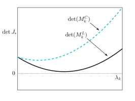
(a)

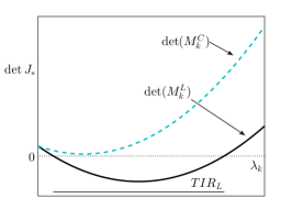
(b)

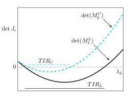
(c)

Figure 1: Turing Instability regions for linear diffusion and cross diffusion cases. (a) There are no regions of strictly negative determinant for both linear and cross diffusion, so that in both cases Turing instability cannot appear. (b) The linear diffusion case has a Turing instability region ($TIR_{L}$), but the determinant of the cross diffusion case is positive for all $\lambda_{k}$, so that the cross diffusion case does not lead to Turing instability. (c) Both cases lead to nonempty Turing instability regions, but the Turing instability region for the cross diffusion ($TIR_{C}$) case is strictly included in the Turing instability region of the linear diffusion case ($TIR_{L}$).

4 Concluding remarks

This paper focuses on the study of two “microscopic” (in terms of time scales) predator-prey models with diffusion, that enable to recover, in a suitable limit, two classical functional responses in the reaction part of the equations and contain a cross-diffusion term. We have also presented rigorous results of convergence of the solutions of these systems towards the solution of the limiting reaction-cross diffusion system.

We first start with two trophic levels, prey and predators, which are further divided into searching predators and handling predators. The former are predators active in the predation process, the latter are resting individuals. Then, we start from a system of three partial differential equations, with standard diffusion terms (a constant times the Laplacian), and with a Lotka-Volterra reaction term. Through a quasi steady-state approximation, we end up with a system of two PDEs with prey and total predator densities as unknowns, in which a Holling-type II functional response appears together with a cross-diffusion term in the predator equation. This means that the diffusion term relative to predators is much more complicated than a constant times Laplacian of $P$ (linear diffusive term), which in some other models is simply added to the reaction part [39]. In particular, the diffusion term obtained in this way depends on the prey biomass and on both the diffusion coefficients of searching and handling predators $d_{2}$ and $d_{3}$. Looking at its expression, the cross-diffusion term reduces the predator diffusion when the prey density increases.

Then we modify the starting model by inserting a competition among predators. With this change we end up after a quasi steady-state approximation with a system of two PDEs for prey and total predator densities, characterized by a Beddington-DeAngelis-like functional response, and a cross-diffusion term in the predator equation.

Also in this case, the limiting system presents a cross-diffusion in the predator equation, which depends on both the diffusion coefficients of searching and handling predators $d_{2}$ and $d_{3}$.

The Turing instability analysis of the limiting equations is studied in Chapter 3. For the first one, it is known that predator-prey models with a prey-dependent trophic function in the reaction part and (standard) linear-diffusion cannot give rise to Turing instability [9]. Even with the cross-diffusion model, no patterns seem to appear under a (biologically reasonable) assumption on the diffusion coefficients. For the second system, in which a Beddington-DeAngelis-like functional response appears, we look for conditions on the parameter values which lead to Turing instability and we compare these Turing instability regions with the ones obtained when the cross-diffusion term is substituted by a standard diffusion. The main point is the fact that the Turing instability region associated to the cross-diffusion system is always strictly included in the Turing instability region of the linear-diffusion system. As a consequence, the use of reaction-diffusion systems for predator-prey interactions of Beddington-DeAngelis type in which standard diffusion is simply added to the reaction terms may lead to an overestimate of the possibility of appearance of patterns (at least in the case when the Beddington-DeAngelis functional response is a consequence of the interactions between searching and handling predators).

It is worth mentioning that in many instances, the introduction of cross-diffusion terms instead of (standard) linear-diffusion terms leads exactly to the opposite result, that is, the increase of the set of parameter values in which patterns develop [32, 33, 40]. Our study leads then to a rather interesting conclusion: pattern formation originating from Turing instability is counteracted by the cross-diffusion term derived by the Quasi-Steady State Approximation.

L.D. acknowledges support from the French “ANR blanche” project Kibord: ANR-13-BS01-0004, and by Université Sorbonne Paris Cité, in the framework of the “Investissements d’Avenir”, convention ANR-11-IDEX-0005. C.S. has been partially supported by the French-Italian program Galileo, project G14-34. Support by INdAM-GNFM is also gratefully acknowledged by F.C. and C.S. The authors are very grateful to Odo Diekmann for his valuable suggestions and remarks that improved the manuscript.

References

• [1] C. S. Holling, The functional response of invertebrate predators to prey density, Memoirs of the Entomological Society of Canada 98 (1966) 5–86.
• [2] V. Ivlev, Experimental Ecology of the Feeding of Fishes, Vol. 42, Yale University Press, New Haven, CT, 1961.
• [3] J. Beddington, Mutual interference between parasites or predators and its effect on searching efficiency, The Journal of Animal Ecology 44 (1975) 331–340.
• [4] D. L. DeAngelis, R. Goldstein, R. O’Neill, A model for trophic interaction, Ecology 56 (1975) 881–892.
• [5] P. A. Abrams, L. R. Ginzburg, The nature of predation: prey dependent, ratio dependent or neither?, Trends in Ecology & Evolution 15 (8) (2000) 337–341.
• [6] A. D. Bazykin, Nonlinear Dynamics of Interacting Populations, Vol. 11, World Scientific, Singapore, 1998.
• [7] X.-C. Zhang, G.-Q. Sun, Z. Jin, Spatial dynamics in a predator-prey model with beddington-deangelis functional response, Physical Review E 85 (2) (2012) 021924.
• [8] M. Haque, Existence of complex patterns in the beddington–deangelis predator–prey model, Mathematical biosciences 239 (2) (2012) 179–190.
• [9] D. Alonso, F. Bartumeus, J. Catalan, Mutual interference between predators can give rise to turing spatial patterns, Ecology 83 (1) (2002) 28–34.
• [10] E. A. McGehee, E. Peacock-López, Turing patterns in a modified lotka–volterra model, Physics Letters A 342 (1) (2005) 90–98.
• [11] H. Malchow, S. V. Petrovskii, E. Venturino, Spatiotemporal patterns in ecology and epidemiology: theory, models, and simulation, Chapman & Hall/CRC London, 2008.
• [12] S. V. Petrovskii, H. Malchow, A minimal model of pattern formation in a prey-predator system, Mathematical and Computer Modelling 29 (8) (1999) 49–63.
• [13] S. V. Petrovskii, H. Malchow, Wave of chaos: new mechanism of pattern formation in spatio-temporal population dynamics, Theoretical population biology 59 (2) (2001) 157–174.
• [14] A. B. Medvinsky, S. V. Petrovskii, I. A. Tikhonova, H. Malchow, B.-L. Li, Spatiotemporal complexity of plankton and fish dynamics, SIAM review 44 (3) (2002) 311–370.
• [15] J. A. Metz, O. Diekmann, The Dynamics of Physiologically Structured Populations, Vol. 68, Springer, 1986.
• [16] S. Geritz, M. Gyllenberg, A mechanistic derivation of the deangelis–beddington functional response, Journal of theoretical biology 314 (2012) 106–108.
• [17] G. Huisman, R. J. De Boer, A formal derivation of the" beddington”functional response, Journal of theoretical biology 185 (3) (1997) 389–400.
• [18] M. Pierre, D. Schmitt, Blowup in reaction-diffusion systems with dissipation of mass, SIAM review 42 (1) (2000) 93–106.
• [19] J. A. Cañizo, L. Desvillettes, K. Fellner, Improved duality estimates and applications to reaction-diffusion equations, Communications in Partial Differential Equations 39 (6) (2014) 1185–1204.
• [20] M. Breden, L. Desvillettes, K. Fellner, Smoothness of moments of the solutions of discrete coagulation equations with diffusion, arXiv preprint arXiv:1511.05733.
• [21] N. Shigesada, K. Kawasaki, E. Teramoto, Spatial segregation of interacting species, Journal of Theoretical Biology 79 (1) (1979) 83–99.
• [22] L. Desvillettes, A. Trescases, New results for triangular reaction cross diffusion system, Journal of Mathematical Analysis and Applications 430 (1) (2015) 32–59.
• [23] H. Murakawa, A relation between cross-diffusion and reaction-diffusion, Citeseer, 2009.
• [24] H. Izuhara, M. Mimura, et al., Reaction-diffusion system approximation to the cross-diffusion competition system, Hiroshima Mathematical Journal 38 (2) (2008) 315–347.
• [25] F. Conforto, L. Desvillettes, Rigorous passage to the limit in a system of reaction-diffusion equations towards a system including cross diffusion, Commun. Math. Sci 12 (3) (2014) 457–472.
• [26] D. Bothe, M. Pierre, The instantaneous limit for reaction-diffusion systems with a fast irreversible reaction, Discr. Cont. Dynam. Systems Ser. S 8 (1) (2011) 49–59.
• [27] D. Bothe, M. Pierre, G. Rolland, Cross-diffusion limit for a reaction-diffusion system with fast reversible reaction, Communications in Partial Differential Equations 37 (11) (2012) 1940–1966.
• [28] D. Hilhorst, M. Mimura, H. Ninomiya, Fast reaction limit of competition-diffusion systems, Handbook of differential equations: evolutionary equations 5 (2009) 105–168.
• [29] D. Hilhorst, R. Van Der Hout, L. Peletier, The fast reaction limit for a reaction-diffusion system, Journal of mathematical analysis and applications 199 (2) (1996) 349–373.
• [30] D. Hilhorst, R. Van Der Hout, L. A. Peletier, Nonlinear diffusion in the presence of fast reaction, Nonlinear Analysis: Theory, Methods & Applications 41 (5) (2000) 803–823.
• [31] G. Rolland, Global existence and fast-reaction limit in reaction-diffusion systems with cross effects, Ph.D. thesis, École normale supérieure de Cachan-ENS Cachan; Technische Universität (Darmstadt, Allemagne) (2012).
• [32] E. Tulumello, M. C. Lombardo, M. Sammartino, Cross-diffusion driven instability in a predator-prey system with cross-diffusion, Acta Applicandae Mathematicae 132 (1) (2014) 621–633.
• [33] M. Iida, M. Mimura, H. Ninomiya, Diffusion, cross-diffusion and competitive interaction, Journal of mathematical biology 53 (4) (2006) 617–641.
• [34] L. Desvillettes, About entropy methods for reaction-diffusion equations, Rivista di Matematica dell’Università di Parma 7 (7) (2007) 81–123.
• [35] L. Desvillettes, K. Fellner, M. Pierre, J. Vovelle, Global existence for quadratic systems of reaction-diffusion, Advanced Nonlinear Studies 7 (3) (2007) 491–511.
• [36] M. Pierre, D. Schmitt, Blowup in reaction-diffusion systems with dissipation of mass, SIAM review 42 (1) (2000) 93–106.
• [37] O. A. Ladyzhenskaia, V. A. Solonnikov, N. N. Ural’tseva, Linear and quasi-linear equations of parabolic type, Vol. 23, American Mathematical Soc., 1988.
• [38] A. Moussa, Some variants of the classical aubin–lions lemma, Journal of Evolution Equations 16 (1) (2016) 65–93.
• [39] R. Durrett, S. Levin, The importance of being discrete (and spatial), Theoretical Population Biology 46 (3) (1994) 363–394.
• [40] G. Gambino, M. C. Lombardo, M. Sammartino, Turing instability and traveling fronts for a nonlinear reaction–diffusion system with cross-diffusion, Mathematics and Computers in Simulation 82 (6) (2012) 1112–1132.