Study of the $\bm{X^{\pm}(5568)}$ state with semileptonic decays of the $\bm{B_{s}^{0}}$ meson

Abstract

We present a study of the $X^{\pm}(5568)$ using semileptonic decays of the $B_{s}^{0}$ meson using the full run II integrated luminosity of 10.4 fb^-1 in proton-antiproton collisions at a center of mass energy of 1.96 TeV collected with the D0 detector at the Fermilab Tevatron Collider. We report evidence for a narrow structure, $X^{\pm}(5568)$, in the decay sequence $X^{\pm}(5568)\to B_{s}^{0}\pi^{\pm}$ where $B_{s}^{0}\rightarrow\mu^{\mp}D_{s}^{\pm}\,\mathrm{X}$, $D_{s}^{\pm}\rightarrow\phi\pi^{\pm}$ which is consistent with the previous measurement by the D0 Collaboration in the hadronic decay mode, $X^{\pm}(5568)\to B^{0}_{s}\pi^{\pm}$ where $B^{0}_{s}\to J/\psi\phi$. The mass and width of this state are measured using a combined fit of the hadronic and semileptonic data, yielding $m=5566.9^{+3.2}_{-3.1}\thinspace{\rm(stat)}^{+0.6}_{-1.2}{\rm\thinspace(syst)}$ MeV/$c^{2}$, $\Gamma=18.6^{+7.9}_{-6.1}{\rm\thinspace(stat)}^{+3.5}_{-3.8}{\rm\thinspace(syst)}$ MeV/$c^{2}$ with a significance of 6.7$\,\sigma$.

I Introduction

Since the creation of the quark model Gell-Mann (1964); Zweig (1964) it was understood that exotic mesons containing more than one quark-antiquark pair are possible. However, for exotic mesons containing only the up, down and strange quarks it has been difficult to make a definitive experimental case for such exotic states, although some persuasive arguments have been made (for recent comprehensive discussions of exotic hadrons containing both light and heavy quarks, see Refs. Maiani et al. (2004); Esposito et al. (2016); Chen et al. (2016); [][]Olsen:2017bmm). Multiquark states that contain heavy quarks can be more recognizable owing to the distinctive decay structure of heavy quark hadrons. The 2003 discovery by the Belle experiment Choi et al. (2003) of the $X(3872)$ in the channel $B^{\pm}\to K^{\pm}X(\to\pi^{+}\pi^{-}J/\psi)$ was the first candidate exotic meson in which heavy flavor quarks participate. This state was subsequently confirmed in several production and decay modes by ATLAS Aaboud et al. (2017), BaBar Aubert et al. (2005), BES III Ablikim et al. (2014), CDF Acosta et al. (2004), CMS Chatrchyan et al. (2013), D0 Abazov et al. (2004) and LHCb Aaij et al. (2013) Collaborations. Several additional four-quark candidate exotic mesons have since been found, though in many cases not all experiments have been able to confirm their existence.

Four-quark mesons can be generically categorized as either “molecular states” or tetraquark states of a diquark and an anti-diquark. In the example of the $X(3872)$, a molecular state interpretation would be a colorless $D^{0}$ ($c\bar{u}$) and a colorless $\bar{D}^{*0}$ ($u\bar{c}$) in a loosely bound state. Such a state would be expected to lie close in mass to the $D^{0}\bar{D}^{*0}$ threshold. The tetraquark mode of a colored diquark ($cu$) and colored anti-diquark ($\bar{c}\bar{u}$) is more strongly bound by the exchange of gluons and would be expected to have a mass somewhat below the $D^{0}$$\bar{D}^{*0}$ threshold. In many cases, interpretations of four-quark mesons as pure molecular or tetraquark states are difficult and more complex mechanisms may be required Esposito et al. (2016); Chen et al. (2016); Olsen et al. (2018). The firm identification of multiquark mesons and baryons and the study of their properties are of importance for further understanding of nonperturbative QCD.

Recently the D0 Collaboration presented evidence for a new four-quark candidate that decays to $B^{0}_{s}\pi^{\pm}$ where $B^{0}_{s}$ decays to $J/\psi\phi$ Abazov et al. (2016). This system would be composed of two quarks and two antiquarks of four different flavors: $b,s,u,d$, with either a molecular constitution as a loosely bound $B_{d}^{0}$ and $K^{\pm}$ system or a tightly bound tetraquark such as $(bd)$-$(\bar{s}\bar{u})$, $(bu)$-$(\bar{s}\bar{d})$, $(su)$-$(\bar{b}\bar{d})$, or $(sd)$-$(\bar{b}\bar{u})$ (because the $B^{0}_{s}$ meson is fully mixed, the exact quark anti-quark composition cannot be determined). The mass of $X^{\pm}(5568)$ is about 200 MeV/$c^{2}$ below the $B_{d}^{0}K^{\pm}$ threshold, thus disfavoring a $B_{d}^{0}$-$K^{\pm}$ molecular interpretation.

The $X^{\pm}(5568)$ was previously reported Abazov et al. (2016) with a significance of 5.1 $\sigma$ (including systematic uncertainties and the look-elsewhere effect [Foradescriptionofthelook-elsewhereeffectsee][]lyons2008) in the decay $X^{\pm}(5568)\to B^{0}_{s}(J/\psi\phi)\pi^{\pm}$ in proton-antiproton collisions at a center of mass energy of 1.96 TeV. The ratio of the number of $B_{s}^{0}$ that are from the decay of the $X^{\pm}(5568)$ to all $B_{s}^{0}$ produced was measured to be $\left[8.6\pm 1.9\thinspace{\rm(stat)}\pm 1.4\thinspace{\rm(syst)}\right]\%$. In order to reduce the background, a selection was imposed on the angle between the $B_{s}^{0}$ and $\pi^{\pm}$ (the “cone cut”, $\Delta R=\sqrt{\Delta\eta^{2}+\Delta\phi^{2}}<0.3$ ). Without the cone cut the significance was found to be 3.9 $\sigma$. In addition to increasing the signal-to-background ratio this cone cut limits backgrounds, such as possible excited states of the $B_{c}$ meson, that are not included in the available simulations. Multiple checks were carried out to ensure that the cone cut did not create an anomalous signal [][(andtheSupplementalMaterialat\url{https://journals.aps.org/prl/supplemental/10.1103/PhysRevLett.117.022003}foradditionalfigures)]D0:2016mwd. Varying the cone cut from $\Delta R_{\mathrm{max}}=0.2$ to $0.5$ gave stable fitted masses and resulted in no unexpected changes in the result. The invariant mass spectra of the $B_{s}^{0}$ candidates and charged tracks with kaon or proton mass hypotheses were checked, and no resonant enhancements in these distributions were found. The invariant mass distribution of $B_{d}^{0}\pi^{\pm}$ was also examined with no unexpected resonances or reflections found. Subsequent analyses by the LHCb Collaboration Aaij et al. (2016) and by the CMS Collaboration [][Phys.Rev.Lett.(tobepublished)]Sirunyan:2017ofq have not found evidence for the $X^{\pm}(5568)$ in proton-proton interactions at $\sqrt{s}=7$ and 8 TeV. The CDF Collaboration has recently reported no evidence for $X^{\pm}(5568)$ in proton-antiproton collisions at $\sqrt{s}=1.96$ TeV [][submittedtoPhys.Rev.Lett.]Aaltonen:2017voc with different kinematic coverage than that of Ref. Abazov et al. (2016).

In this article, we present a study of the $X^{\pm}(5568)$ in the decay to $B^{0}_{s}\pi^{\pm}$ using semileptonic $B^{0}_{s}$ decays, $B_{s}^{0}\rightarrow\mu^{+}D_{s}^{-}\,\mathrm{X}$, where $D_{s}^{-}\rightarrow\phi\pi^{-}$, $\phi\to K^{+}K^{-}$, using the full run II integrated luminosity of 10.4 fb^-1 in proton-antiproton collisions at a center of mass energy of 1.96 TeV collected with the D0 detector at the Fermilab Tevatron Collider. Charge conjugate states are assumed. Here X includes the unseen neutrino and possibly a photon or $\pi^{0}$ from a $D_{s}^{\ast}$ decay or other hadrons from the $B^{0}_{s}$ decay. The decay process is illustrated in Fig. 1. The semileptonic decay channel has a higher branching fraction than the hadronic channel ($B_{s}^{0}\rightarrow J/\psi\phi$). However the presence of the unmeasured neutrino in the final state deteriorates the mass resolution of the signal. Still, a good mass resolution for the $X^{\pm}(5568)$ can be obtained in the semileptonic channel for events with a large invariant mass of the $\mu^{+}D_{s}^{-}$ system, yielding a comparable number of selected $B^{0}_{s}$ candidates in the two channels. The backgrounds in the semileptonic channel are independent of, but somewhat larger than, those in the hadronic channel. The character of possible reflections of other resonant structures is quite different in the semileptonic and hadronic channels. Thus observation of the $X^{\pm}(5568)$ in the semileptonic decay channel enables an independent confirmation of its existence. We report here the results of the search for the $X^{\pm}(5568)$ in the semileptonic channel, as well as a combination of the results in the hadronic and semileptonic channels.

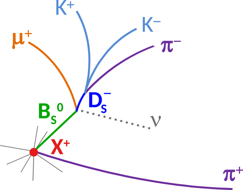
Figure 1: An illustration of the decay $X^{+}(5568)\to B^{0}_{s}\pi^{+}$ where $B_{s}^{0}\rightarrow\mu^{+}D_{s}^{-}\,\mathrm{X}$ in the plane perpendicular to the beam.

II D0 detector

The detector components most relevant to this analysis are the central tracking and the muon systems. The D0 detector has a central tracking system consisting of a silicon microstrip tracker (SMT) and a central fiber tracker (CFT), both located within a 2 T superconducting solenoidal magnet Abazov et al. (2006); Angstadt et al. (2010). The SMT has a design optimized for tracking and vertexing for pseudorapidity of $|\eta|<3$. For charged particles, the resolution on the distance of closest approach as provided by the tracking system is approximately 50 $\mu$m for tracks with $p_{T}\approx 1$ GeV/$c$, where $p_{T}$ is the component of the momentum perpendicular to the beam axis. It improves asymptotically to 15 $\mu$m for tracks with $p_{T}>10$ GeV/$c$. Preshower detectors and electromagnetic and hadronic calorimeters surround the tracker. A muon system, positioned outside the calorimeter, covering $|\eta|<2$ consists of a layer of tracking detectors and scintillation trigger counters in front of 1.8 T iron toroidal magnets, followed by two similar layers after the toroids Abazov et al. (2005).

III Event reconstruction and selection

The $B_{s}^{0}\rightarrow\mu^{+}D_{s}^{-}\,\mathrm{X}$  selection requirements have been chosen to optimize the mass resolution of the $B^{0}_{s}\pi^{+}$ system and to minimize background from random combinations of tracks from muons and charged hadrons. The selection criteria are based on those used in Ref. Abazov et al. (2013) with the cut on the $B^{0}_{s}$ isolation removed and have been selected by maximizing the significance of the signal.

The data were collected with a suite of single and dimuon triggers (approximately 95% of the sample is recorded using single muon triggers). The selection and reconstruction of $\mu^{+}D_{s}^{-}$ decays requires tracks with at least two hits in both the CFT and SMT.

The muon is required to have hits in at least two layers of the muon system, with segments reconstructed both inside and outside the toroid. The muon track segment is required to be matched to a track found in the central tracking system that has transverse momentum $3<p_{T}<25$ GeV/$c$.

The $D_{s}^{-}\rightarrow\phi\pi^{-}$; $\phi\rightarrow K^{+}K^{-}$ decay is selected as follows. The two particles from the $\phi$ decay are assumed to be kaons and are required to have $p_{T}>1.0$ GeV/$c$, opposite charge and an invariant mass $1.012<m(K^{+}K^{-})<1.03$ GeV/$c^{2}$. The charge of the third particle, assumed to be a pion, has to be opposite to that of the muon. This particle is required to have transverse momentum $0.5<p_{T}<25$ GeV/$c$. The mass of the three particles must satisfy $1.91<m(K^{+}K^{-}\pi^{-})<2.03$ MeV$/c^{2}$. The three tracks are combined to form a common $D_{s}^{-}$ decay vertex using the algorithm described in Ref. Abdallah et al. (2004). The $D^{-}_{s}$ vertex is required to be displaced from the $p\bar{p}$ primary interaction vertex (PV) in the transverse plane with a significance of at least three standard deviations. The cosine of the angle between the $D^{-}_{s}$ momentum and the vector from the PV to the $D^{-}_{s}$ decay vertex is required to be greater than 0.9.

The trajectories of the muon and $D^{-}_{s}$ candidate are required to be consistent with originating from a common vertex (assumed to be the $B^{0}_{s}$ semileptonic decay vertex). The cosine of the angle between the combined $\mu^{+}D^{-}_{s}$ transverse momentum, an approximation of the $B^{0}_{s}$ direction, and the direction from the PV to the $B^{0}_{s}$ decay vertex has to be greater than 0.95. The $B^{0}_{s}$ decay vertex has to be displaced from the PV in the transverse plane with a significance of at least four standard deviations. The transverse momentum of the $\mu^{+}D_{s}^{-}$ system is required to satisfy the condition $p_{T}>10$ GeV/$c$ to suppress backgrounds. To minimize the effect of the neutrino in the final state the effective mass is limited to $4.5\,$GeV$/c^{2}\,<m(\mu^{+}D_{s}^{-})<m(B^{0}_{s})$.

The impact parameters (IP)  with respect to the PV of the four tracks from the $B^{0}_{s}$ decay are required to satisfy the following criteria: the two-dimensional (2D) IPs of the tracks of the muon and the pion from the $D_{s}^{-}$ decay are required to be at least 50 $\mu$m to reject tracks emerging promptly from the PV (this requirement is not applied to the tracks associated with the charged kaons since the mass requirements provide satisfactory background suppression). The three-dimensional (3D) IPs of all four tracks are required to be less than 2 cm to suppress combinations with tracks emerging from different $p\bar{p}$ vertices reconstructed in the same beam crossing.

The $m(K^{+}K^{-}\pi^{\pm})$ distribution of the candidates that pass these cuts [except $1.91<m(K^{+}K^{-}\pi^{-})<2.03$ MeV$/c^{2}$] is shown in Fig. 2, where the invariant mass distribution in data is compared to a fit using a function which includes three terms: a second order polynomial used to describe combinatorial background, a Gaussian used to model the $D^{-}$ peak, and a double Gaussian with similar, but different masses and widths used to model the $D_{s}^{-}$ peak.

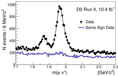
Figure 2: The $K^{+}K^{-}\pi^{\pm}$ invariant mass distribution for the $\mu^{\pm}\phi\pi^{\mp}$ sample (right sign) with the solid curve representing the fit. The lower mass peak is due to the decay $D^{\pm}\rightarrow\phi\pi^{\pm}$ and the second peak is due to the $D_{s}^{\pm}$ decay. The blue histogram below the data points is the invariant mass distribution for the same-sign sample, $\mu^{\pm}\phi\pi^{\pm}$.

The selection criteria for the pion in the $B^{0}_{s}\pi^{\pm}$ combination have been chosen to match those used in the hadronic analysis. The track representing the pion is required to have transverse momentum $0.5<p_{T}<25$ GeV/$c$ (the upper limit is applied to reduce background). The pion and the $B^{0}_{s}$ candidate are combined to form a vertex that is consistent with the PV. The pion is required to be associated with the PV and have a 2D IP of at most 200 $\mu$m and a 3D IP that is less than 0.12 cm. Events with more than 20 $B^{0}_{s}\pi^{\pm}$ candidates are rejected. The most likely number of candidates per event is 5.1 and only about 0.1% of the events have more than 20 candidates per event. To improve the resolution of the invariant mass of the $B^{0}_{s}\pi^{\pm}$ system we define the invariant mass as $m(B^{0}_{s}\pi^{\pm})=m(\mu^{+}D_{s}^{-}\pi^{\pm})-m(\mu^{+}D_{s}^{-})+m(B^{0}_{s})$ where $m(B^{0}_{s})=5.3667$ GeV/$c^{2}$ Patrignani et al. (2016). We study the mass distribution in the range $5.506<m(B^{0}_{s}\pi^{\pm})<5.906$ GeV/$c^{2}$. When using the hadronic data from Ref. Abazov et al. (2016) in this paper we use the same mass range as the semileptonic data instead of the slightly shifted mass range used in the original analysis ($5.5<m(B^{0}_{s}\pi^{\pm})<5.9$ GeV/$c^{2}$). The semileptonic data are studied with and without a cone cut which is used to suppress background, in which the angle between the $\mu^{+}D_{s}^{-}$ system and $\pi^{\pm}$ is required to satisfy $\Delta R=\sqrt{\Delta\eta^{2}+\Delta\phi^{2}}<0.3$. The resulting invariant mass distributions for the semileptonic channel are shown in Fig. 3.

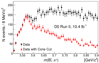
Figure 3: The $m(B^{0}_{s}\pi^{\pm})$ distribution for the semileptonic data with (red upward triangles) and without (black downward triangles) the cone cut. Below 5.56 GeV/$c^{2}$ the red and black points have the same values.

The selection cuts and resulting kinematics for the hadronic and semileptonic channels are quite similar. The requirement that muons be seen outside the toroids means that the minimum $p_{T}$ for the $J/\psi$ in the hadronic channel is about 4 GeV and about 3  GeV for the single muon in the semileptonic channel. The minimum $p_{T}$ for the additional pion is 0.5 GeV for both the hadronic and semileptonic channels. For both channels, we require the minimum $p_{T}(B^{0}_{s}\pi)$ to be greater than 10 GeV and the average $p_{T}(B^{0}_{s}\pi)$ for events with $m(B_{s}\pi)\approx 5.5$ GeV is $\approx 17$  GeV. For both channels the $B^{0}_{s}\pi$ candidates are in the range of $-2<\eta<2$ and more than half of the events have a muon with $|\eta|>1$.

IV Monte Carlo simulation, Background Modeling and parameterization

Monte Carlo (MC) samples are generated using the pythia Sjostrand et al. (2006) event generator, modified to use evtgen [][fordetailsseehttp://www.slac.stanford.edu/$∼$lange/EvtGen]Lange:2001uf for the decay of hadrons containing $b$ or $c$ quarks. The generated events are processed by the full detector simulation chain. Data events recorded in random beam crossings are overlaid on the MC events to simulate the effect of additional collisions in the same or nearby bunch crossings. The resulting events are then processed with the same reconstruction and selection algorithms as used for data events.

The MC sample for $X^{\pm}(5568)$ signal is generated by modifying the mass of the $B^{\pm}$ meson and forcing it to decay to $B^{0}_{s}\pi^{\pm}$ using an isotropic S-wave decay model. The $X^{\pm}(5568)$ is simulated with zero width and zero lifetime. The resulting $K^{+}K^{-}\pi^{-}$ and $B^{0}_{s}\pi^{\pm}$ invariant mass distributions are shown in Fig. 4 with all selection requirements.

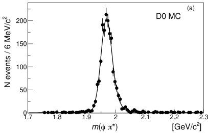
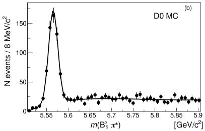
Figure 4: MC simulation of $X^{\pm}(5568)\to B^{0}_{s}\pi^{\pm}$ where $B_{s}^{0}\rightarrow\mu^{+}D_{s}^{-}\,\mathrm{X}$ and the width of the $X^{\pm}(5568)$ is zero. The invariant mass distributions a) $m(K^{+}K^{-}\pi^{-})$ and b) $m(B^{0}_{s}\pi^{+})$ are shown. The background in the $m(B^{0}_{s}\pi^{+})$ distribution is produced by the combination of a random charged track with the $B^{0}_{s}$ meson.

The signal component of the $K^{+}K^{-}\pi^{\pm}$ invariant mass distribution (Fig. 4 a) is modeled by two Gaussian functions and the background by a second-order polynomial. The signal of the $m(B^{0}_{s}\pi^{\pm})$ distribution (Fig. 4 b) is well modeled with a single Gaussian and the background with a third-order polynomial times an exponential. Using the results of these fits the reconstruction efficiency of the charged pion in the decay $X^{\pm}(5568)\to B^{0}_{s}\pi^{\pm}$ is $\left[32.0\pm 1.8\thinspace{\rm(stat)}\pm 1.6\thinspace{\rm(syst)}\right]\%$ for $p_{T}(\mu^{+}D_{s}^{-})>10$ GeV/$c$ where the systematic uncertainty represents the expected differences between the reconstruction efficiencies for low-momentum tracks in the MC simulation and data.

It is not possible to create a model of the background that is based only on data. Since the $X^{\pm}(5568)$ decays to $B^{0}_{s}$ mesons, any data sample that includes $B^{0}_{s}$ decays will also include the signal and is unsuitable for modeling the background. Hence, we use MC-generated $B^{0}_{s}$ events that result from known particles that have decays that include a $B^{0}_{s}$ in the decay chain, combined with data events where the muon has the same sign as the $D_{s}^{-}$ candidate (SS events). MC event generators do not include all possible states as in many cases they have not been experimentally observed. For example, $b\bar{c}$ resonances decaying to $B^{0}_{s}$ mesons could contribute to our sample.

There are two distinct sources of background in this analysis. The first occurs when an $X^{\pm}(5568)$ candidate is reconstructed from a real $\mu^{+}$ and $D_{s}^{-}$ together with a random charged track. This background is modeled using MC samples.

The background MC sample is generated using the pythia inclusive heavy flavor production model and events are selected that contain at least one muon and a $D_{s}^{\mp}\rightarrow\phi\pi^{\mp}$ decay where $\phi\rightarrow K^{+}K^{-}$. To correct for the difference in lifetimes in the MC simulation and data, a weighting is applied to all nonprompt events in the simulation, based on the generated lifetime of the $B$ candidate, to give the world-average $B$ hadron lifetimes Patrignani et al. (2016). To correct for the effects of the trigger selection and the reconstruction in data, we also weight each MC event so that the transverse momenta of the reconstructed muon and the $\mu^{+}D_{s}^{-}$ system agree with those in the data. The $p_{T}$ distribution of the $B^{0}_{s}\pi^{\pm}$ system is altered significantly by the weighting as shown in Fig. 5(a). However, the effect is relatively small for the $B^{0}_{s}\pi^{\pm}$ mass distribution as seen in Fig. 5(b).

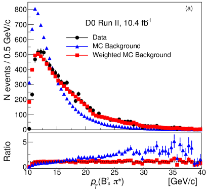
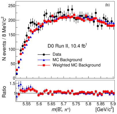
Figure 5: The MC background distribution, without the cone cut, before and after weighting is compared with data (black points). The unweighted MC simulationis in blue and the weighted is in red. The a) $p_{T}(B^{0}_{s}\pi^{\pm})$ and b) invariant mass distributions $m(B^{0}_{s}\pi^{\pm})$ are shown. The excess in the data around $m(B^{0}_{s}\pi^{\pm})=5565$ MeV/c is the $X^{\pm}(5568)$ signal. The lower panels show the ratio between the data and corresponding MC simulation.

The second source of background is the combinatorial background that occurs when a $X^{\pm}(5568)$ candidate is reconstructed from a spurious $D_{s}^{-}$ candidate formed from three random charged tracks that form a vertex. This background is modeled using data events where the muon has the same sign as the $D_{s}^{-}$ candidate (SS events).

In Fig. 6(b) we compare the reweighted MC background simulation, smoothed using one iteration of the 353QH algorithm [J.Friedman; ][wherefor$n$datapointsthesmoothed$i^\mathrm{th}$point$y_s(i)$isgivenby$y_s(i)=0.25y(i-1)+0.5y(i)+0.25y(i+1)$for$i=2; n-1$and$y_s(1)=y(1)$and$y_s(n)=y(n)$.]Proceedings:1974sfa, with the SS data for the no cone cut case. These two backgrounds are in good agreement since the $\chi^{2}$ between them is 50 for 50 bins. We therefore choose to use the MC background shape only, for the data without the cone cut. In Fig. 6(a) we make the same comparison for the data with the cone cut. In this case, $\chi^{2}$ = 77 for the 50 bins, and we therefore need to model the background shape with a combination of the MC and SS backgrounds.

To construct the background sample for the data with the cone cut the fraction of MC and SS backgrounds need to be determined. This is found by fitting the data with a combination of the MC and SS with the fraction of MC events as a free parameter in the sideband mass range $5.506<m(B^{0}_{s}\pi^{\pm})<5.55$ and $5.650<m(B^{0}_{s}\pi^{\pm})<5.906$ GeV/$c^{2}$. The best agreement is found when the MC fraction is $\left(62\pm 2\right)\%$.

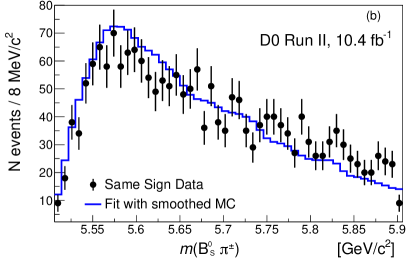
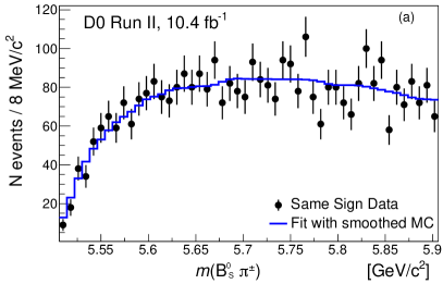
Figure 6: The comparison of the $m(B_{s}^{0}\pi^{\pm})$ background only distributions a) with the cone cut and b) without the cone cut, obtained using the weighted MC (histogram) and from the same sign data samples (points with error bars). The fluctuations in the number of MC events with the cone cut are due to the weighting procedure and the size of the sample.

We choose the background parametrization for the invariant mass distribution, both with and without the cone cut, to be

$$F_{\mathrm{bgr}}(m)={} \left(C_{1}m_{0}+C_{2}m_{0}^{2}+C_{3}m_{0}^{3}+C_{4}m_{0}^{4}\right)$$

$$\times\exp\left(C_{5}m_{0}+C_{7}m_{0}^{2}\right),$$ (1)

where $m=m(B_{s}^{0}\pi^{\pm})$, $m_{0}=m-m_{\mathrm{th}}$ and $m_{\mathrm{th}}=5.5063$ GeV$/c^{2}$ is the mass threshold. Our baseline choice of Eq. (IV) gives an equivalently good description of the background as that used in Ref. Abazov et al. (2016) [Eq. (IV)]. It has the advantages of having one fewer parameter and being zero at the mass threshold.

Three alternative parametrizations are used to model the background. The first is that used in Ref. Abazov et al. (2016),

$$F_{\mathrm{bgr}}(m)={} \left(C_{1}+C_{2}m_{\Delta}^{2}+C_{3}m_{\Delta}^{3}+C_{4}m_{\Delta}^{4}\right)$$

$$\times\exp\left(C_{5}+C_{6}m_{\Delta}+C_{7}m_{\Delta}^{2}\right),$$ (2)

where $m_{\Delta}=m-\Delta$ and $\Delta=5.500$ GeV$/c^{2}$. The second is the ARGUS function Albrecht et al. (1990) which is specifically constructed to describe background near a threshold

$$F_{\mathrm{bgr}}(m)=m\left(\frac{m^{2}}{m_{\mathrm{th}}^{2}}-1\right)^{C_{1}}\exp\left(C_{2}m\right).$$ (3)

The third alternative model used to fit the background is the MC histogram (or combined MC and SS data) smoothed using one iteration of the 353QH algorithm [J.Friedman; ][wherefor$n$datapointsthesmoothed$i^\mathrm{th}$point$y_s(i)$isgivenby$y_s(i)=0.25y(i-1)+0.5y(i)+0.25y(i+1)$for$i=2; n-1$and$y_s(1)=y(1)$and$y_s(n)=y(n)$.]Proceedings:1974sfa.

The ARGUS function is not used as an alternate parametrization in the semileptonic data with the cone cut, because the fit to background is strongly disfavored (the $\chi^{2}$ of the fit to the MC background is 145 compared with approximately 50 for the alternate functions). The $\chi^{2}$ per number of degrees of freedom ($\mathrm{ndf}$) for the four representations of the background are shown in Table 1.

We choose the background description of Eq. (IV) as the baseline. The alternative functions and the smoothed MC are used to estimate the systematic uncertainty on the background shape. The $m(B^{0}_{s}\pi^{\pm})$ background model distribution along with the fit using Eq. (IV) is presented in Fig. 7.

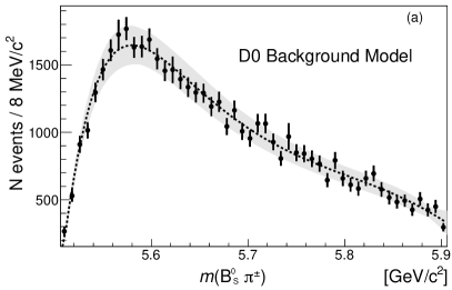
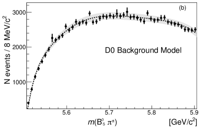
Figure 7: The background model produced according to the procedure described in the text is shown along with background function (IV) (dotted line) (a) with and (b) without the cone cut. The gray band shows the systematic uncertainties on the background model (see Sec. VI D).

Table 1: Fit results for different parametrizations to the background model.

Background function	$\chi^{2}/$ndf
	Cone cut	No cone cut
Eq. (1)	51.0/(50-6) = 1.2	48.1/(50-6) = 1.1
Eq. (2)	42.9/(50-7) = 1.0	48.1/(50-7) = 1.1
Eq. (3)	145/(50-2) = 3.0	38.3/(50-2) = 0.8
Smoothed background	33.8/(50-1) = 0.7	30.9/(50-1) = 0.6

V Signal Mass Resolution

We calculate the mass of the $B^{0}_{s}\pi^{\pm}$ system using the quantity

$$m(B^{0}_{s}\pi^{\pm})=m(\mu^{\pm}D_{s}^{\mp}\pi^{\pm})-m(\mu^{\pm}D_{s}^{\mp})+m(B^{0}_{s}).$$ (4)

Before carrying out the search for the $X^{\pm}(5568)$ in the semileptonic channel we ensure that it is an unbiased and precise estimator of the mass of the $B^{0}_{s}\pi^{\pm}$ system. This is studied by simulating the two body decay $X(5568)^{\pm}\to B^{0}_{s}\pi^{\pm}$ where $B_{s}^{0}\rightarrow\mu^{\pm}D_{s}^{\mp}\,\mathrm{X}$, starting with a range of input masses $\widetilde{m}(B^{0}_{s}\pi^{\pm})$. Following the decay chain $B_{s}^{0}\rightarrow\mu^{\pm}D_{s}^{\mp}\,\mathrm{X}$and forming the invariant masses $m(\mu^{\pm}D_{s}^{\mp}\pi^{\pm})$ and $m(\mu^{\pm}D_{s}^{\mp})$ are found. Then $m(B^{0}_{s}\pi^{\pm})$ is calculated and compared to the input mass $\widetilde{m}(B^{0}_{s}\pi^{\pm})$.

To evaluate how well the mass approximation works to compensate for the missing neutrino, we model the decay with a toy MC that simulates the virtual $W$ in $B^{0}_{s}\to D_{s}^{\mp}+W^{\ast}$ with an isotropic distribution of $\mu$ and $\nu$ in the $W$ boson rest frame. The resulting resolution of a zero width resonance due to the presence of the neutrino is modeled by a Gaussian. The width varies according to $\widetilde{m}(B^{0}_{s}\pi^{\pm})$ as illustrated by the solid line in Fig. 8.

The mass resolution for the D0 detector of a state decaying into five reconstructed charged particles with a similar kinematic range as in this study is measured using the MC simulation and is given by a Gaussian function of width 3.85 MeV/$c^{2}$. The $m(B^{0}_{s}\pi^{\pm})$ resolution function is obtained by convoluting the Gaussian tracking resolution and the smearing resolution resulting from the missing neutrino. The resulting combined resolution, the dashed line in Fig. 8, can be approximated by

$$\sigma_{\mathrm{SL}}=\left[3.85+60.93(m_{0}^{0.85})\right]\,\mathrm{MeV}/c^{2}$$ (5)

where $m_{0}$ has the same definition as in Eq. (IV). These studies show that the difference between $m(B^{0}_{s}\pi^{\pm})$ and $\widetilde{m}(B^{0}_{s}\pi^{\pm})$ is less than 1 MeV/$c^{2}$ in the search region. This is confirmed with the signal MC sample.

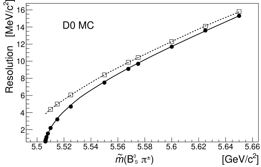
Figure 8: The resolution for a zero width resonance as a function of $\widetilde{m}(B^{0}_{s}\pi^{\pm})$. The solid circles and the solid line show the effect of the missing neutrino and the open squares and dashed line show the convolution of the resolution due to the missing neutrino convolved with the 3.85 MeV/$c^{2}$ detector mass resolution.

VI Signal Fit Function

The $X^{\pm}(5568)$ resonance is modeled by a relativistic Breit-Wigner function convolved with a Gaussian detector resolution function given in Eq. (5), $F_{\rm sig}(m,m_{X},\Gamma{{}_{X}})$, where $m_{X}$ and $\Gamma_{X}$ are the mass and the width of the resonance.

The fit function has the form

$$F=f_{\rm sig}F_{\rm sig}(m,m_{X},\Gamma{{}_{X}})+f_{\rm bgr}F_{\rm bgr}(m),$$ (6)

where $f_{\rm sig}$ and $f_{\rm bgr}$ are normalization factors. The shape parameters in the background term $F_{\rm bgr}$ are fixed to the values obtained from fitting the MC background distribution (see Fig. 7).

We use the Breit-Wigner parametrization appropriate for an S-wave two-body decay near threshold:

$$BW(m)\propto\frac{m_{X}^{2}\Gamma(m)}{(m_{X}^{2}-m^{2})^{2}+m_{X}^{2}\Gamma{{}^{2}}(m)}.$$ (7)

The mass-dependent width $\Gamma(m)=\Gamma_{X}\cdot(q_{1}/q_{0})$, where $q_{1}$ and $q_{0}$ are the magnitudes of momenta of the $B_{s}^{0}$ meson in the rest frame of the $B_{s}^{0}\pi^{\pm}$ system at the invariant mass equal to $m$ and $m_{X}$, respectively.

VII $\bm{X^{\pm}(5568)}$ semileptonic fit results

In the fit to the semileptonic data with the cone cut shown in Fig. 9(a), the normalization parameters $f_{\rm sig}$ and $f_{\rm bgr}$ and the Breit-Wigner parameters $m_{X}$ and $\Gamma{{}_{X}}$ are allowed to vary. The fit yields the mass and width of $m_{X}=5566.4^{+3.4}_{-2.8}$ MeV/$c^{2}$, $\Gamma{{}_{X}}=2.0^{+9.5}_{-2.0}$ MeV/$c^{2}$, the number of signal events, $N=121^{+51}_{-34}$, and a $\chi^{2}=34.9$ for 46 degrees of freedom. The local statistical significance of the signal is defined as $\sqrt{-2\,{\rm ln}({\cal{L}}_{0}/{\cal{L}}_{\mathrm{max}})}$, where ${\cal{L}}_{\mathrm{max}}$ and ${\cal{L}}_{0}$ are likelihood values at the best-fit signal yield and the signal yield fixed to zero obtained from a binned maximum-likelihood fit. The $p$-value of the background only fit is $2.1\times 10^{-5}$ and the local statistical significance is 4.3 $\sigma$.

In the fit to the semileptonic data without the cone cut shown in Fig. 9(b), the mass and width of $m_{X}=5566.7^{+3.6}_{-3.4}$ MeV/$c^{2}$, $\Gamma{{}_{X}}=6.0^{+9.5}_{-6.0}$ MeV/$c^{2}$, the number of signal events, $N=139^{+51}_{-63}$, and a $\chi^{2}=30.4$ for 46 degrees of freedom. The $p$-value of the background only fit is $7.7\times 10^{-6}$ and the local statistical significance is 4.5 $\sigma$. The fit results, both for the cone cut and no cone cut cases, are given in Table 2 and for various background parametrizations in Table 3. The $X^{\pm}(5568)$ parameters for the cone cut and no cone cut cases are consistent.

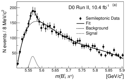
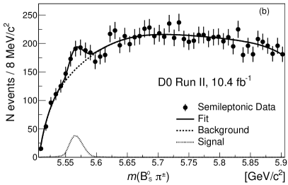
Figure 9: The $m(B^{0}_{s}\pi^{\pm})$ distribution (a) with and (b) without the cone cut. The fitting function is superimposed (see text for details).

Table 2: Results for the fit to the semileptonic data sets (see Fig. 9).

	Cone cut	No cone cut
Fitted mass, MeV/$c^{2}$	$5566.4^{+3.4}_{-2.8}\,\mbox{(stat)}^{+1.5}_{-0.6}\,\mbox{(syst)}$	$5566.7^{+3.6}_{-3.4}\,\mbox{(stat)}^{+1.0}_{-1.0}\,\mbox{(syst)}$
Fitted width, MeV/$c^{2}$	$2.0^{+9.5}_{-2.0}\,\mbox{(stat)}^{+2.8}_{-2.0}\,\mbox{(syst)}$	$6.0^{+9.5}_{-6.0}\,\mbox{(stat)}^{+1.9}_{-4.6}\,\mbox{(syst)}$
Fitted number of signal events	$121^{+51}_{-34}\,\mbox{(stat)}^{+9}_{-28}\,\mbox{(syst)}$	$139^{+51}_{-63}\,\mbox{(stat)}^{+11}_{-32}\,\mbox{(syst)}$
$\chi^{2}/$ndf	$34.9/(50-4)$	$30.4/(50-4)$
$p$-value	$2.1\times 10^{-5}$	$7.7\times 10^{-6}$
Local significance	$4.3\,\sigma$	$4.5\,\sigma$
Significance including systematic uncertainties	$3.2\,\sigma$	$3.4\,\sigma$

Table 3: Semileptonic data fits for the different background parametrizations.

	Equation (IV)	Equation (IV)	Equation (3)	Smoothed MC simulation
Cone Cut
Fitted mass, MeV/$c^{2}$	$5566.4^{+3.4}_{-2.8}$	$5566.1^{+3.7}_{-3.2}$	…	$5567.1^{+4.4}_{-3.3}$
Fitted width, MeV/$c^{2}$	$2.0^{+9.5}_{-2.0}$	$1.0^{+12.8}_{-1.0}$	…	$1.2^{+12.9}_{-1.2}$
Fitted number of signal events	$121^{+51}_{-34}$	$98^{+52}_{-29}$	…	$95^{+51}_{-30}$
$\chi^{2}/$ndf	$34.9/(50-4)$	$43.2/(50-4)$	…	$50.5/(50-4)$
Local significance	$4.3\,\sigma$	$3.6\,\sigma$	…	$3.5\,\sigma$
No Cone Cut
Fitted mass, MeV/$c^{2}$	$5566.7^{+3.6}_{-3.4}$	$5566.2^{+4.2}_{-4.1}$	$5566.0^{+3.6}_{-3.4}$	$5566.1^{+4.5}_{-4.5}$
Fitted width, MeV/$c^{2}$	$6.0^{+9.5}_{-6.0}$	$6.0^{+12.0}_{-6.0}$	$6.5^{+8.9}_{-6.5}$	$10^{+13}_{-10}$
Fitted number of signal events	$139^{+51}_{-63}$	$116^{+52}_{-48}$	$146^{+51}_{-54}$	$130^{+56}_{-48}$
$\chi^{2}/$ndf	$30.4/(50-4)$	$50.3/(50-4)$	$43.8/(50-4)$	$44.8/(50-4)$
Local significance	$4.5\,\sigma$	$3.7\,\sigma$	$4.7\,\sigma$	$3.8\,\sigma$

VII.1 Systematic uncertainties

Systematic uncertainties (Table 4) are obtained for the measured values of the mass, width and event yield of the $X^{\pm}(5568)$ signal. The dominant uncertainty is due to (i) the description of the background shape. We evaluate this systematic uncertainty by using the alternative paramaterizations of the background, Eqs. (2), (3) and the smoothed MC histogram and finding the maximal deviations from the nominal fit.

The effect of (ii) the MC weighting is estimated by creating 1000 background samples where the weights have been randomly varied based on the uncertainties in the weighting procedure.

Other sources of systematic uncertainty are evaluated by (iii) varying the energy scale in the MC sample relative to the data by $\pm$1 MeV/$c^{2}$, (iv) varying the mass resolution of the $X^{\pm}(5568)$ either by $\pm$1 MeV/$c^{2}$ around the mean value, or by using a constant resolution of 11.1 MeV/$c^{2}$ obtained from the MC simulation of the $X^{\pm}(5568)$ signal, (v) using a P-wave relativistic Breit-Wigner function, and (vi) estimating the shift of the fitted mass peak due to the missing neutrino.

Systematic uncertainties are summarized in Table 4. The uncertainties are added in quadrature separately for positive and negative values to obtain the total systematic uncertainties for each measured parameter. The results including systematic uncertainties are given in Table 2.

Table 4: Systematic uncertainties for the $X^{\pm}(5568)$ state mass, width and the event yield obtained from the semileptonic data.

Source	Mass, MeV/$c^{2}$	Width, MeV/$c^{2}$	event yield, events
Cone Cut
(i) Background shape description	+0.7  ; $-0.3$	+0.0  ; $-1.0$	+0.0  ; $-26.6$
(ii) Background reweighting	+0.1  ; $-0.1$	+0.4  ; $-0.4$	+3.9  ; $-4.2$
(iii) $B_{s}^{0}$ mass scale, MC simulation and data	+0.1  ; $-0.3$	+0.8  ; $-1.0$	+5.1  ; $-7.8$
(iv) Detector resolution	+0.9  ; $-0.0$	+2.7  ; $-1.0$	+6.5  ; $-0.0$
(v) P-wave Breit-Wigner	+0.0  ; $-0.4$	+0.0  ; $-1.0$	+0.0  ; $-3.7$
(vi) Missing neutrino effect	+1.0  ; $-0.0$	-	-
Total	+1.5  ; $-0.6$	+2.8  ; $-2.0$	+9.1  ; $-28.3$
No Cone Cut
(i) Background shape description	+0.0  ; $-0.7$	+0.7  ; $-2.5$	+4.8  ; $-28.0$
(ii) Background reweighting	+0.1  ; $-0.1$	+0.7  ; $-0.7$	+5.0  ; $-5.0$
(iii) $B_{s}^{0}$ mass scale, MC simulation and data	+0.3  ; $-0.5$	+1.0  ; $-1.4$	+7.5  ; $-9.6$
(iv) Detector resolution	+0.0  ; $-0.5$	+1.3  ; $-2.6$	+3.7  ; $-6.4$
(v) P-wave Breit-Wigner	+0.0  ; $-0.2$	+0.0  ; $-2.4$	+0.0  ; $-7.0$
(vi) Missing neutrino effect	+1.0  ; $-0.0$	-	-
Total	+1.0  ; $-1.0$	+1.9  ; $-4.6$	+10.9  ; $-31.5$

VII.2 Significance

Since we are seeking to confirm the result presented in Ref. Abazov et al. (2016) we do not apply a correction for a look elsewhere effect. The systematic uncertainties are treated as nuisance parameters to construct a prior predictive model Patrignani et al. (2016); Giunti (1999) of our test statistic. When the systematic uncertainties are included, the significance of the observed semileptonic signal with the cone cut is 3.2 $\sigma$ ($p$-value = $1.4\times 10^{-3}$). The significance of the semileptonic signal without the cone is 3.4 $\sigma$ ($p$-value = $6.4\times 10^{-4}$).

VII.3 Closure tests

We have tested the accuracy of the fitting procedure using toy MC event samples constructed with input mass and width of 5568.3 and 21.9 MeV$/c^{2}$ respectively, with the number of input signal events varied in steps of 25 between 75 and 350. At each number of input signal events, 10,000 pseudoexperiments were generated. The signals are modeled with a relativistic Breit-Wigner function convolved with a Gaussian function representing the appropriate detector resolution. The background distribution is based on Eq. (IV). For each trial the fitting procedure is performed to obtain the mass and width and the number of semileptonic signal events. The results of each set of trials is fitted with a Gaussian to determine the mean and the uncertainty in the number of signal events, the mass and the width (see Table 5). The number of fitted signal events vs. the number of injected signal events for the semileptonic samples are plotted in Fig. 10.

For the ensembles with a number of input events similar to that observed in data, there is a slight overestimate of the yield and fitted mass, and the width is underestimated. This width reduction is in agreement with the results of the fits to data (Sec. VII), and indicate that the semileptonic data are not sensitive to the width. These effects are accounted for in the calculation of the significance.

Table 5: Mean values and uncertainties for fitted number of events, mass and width from Gaussian fits to corresponding distributions from 10,000 trials with the cone cut. Also given is the expected statistical uncertainties on the fitted number of events, $\Delta$($N_{\mathrm{fit}}(\mathrm{sl})$), and the expected uncertainties on the measurement of the width, $\Delta(\Gamma_{X})$ MeV/$c^{2}$. A range of signals with 75, 100, 125, 150, 175 and 200 signal events, mass $m_{x}=5568.3$ MeV$/c^{2}$ and width $\Gamma_{X}=21.9$ MeV$/c^{2}$ have been simulated. Background parameterization Eq. (IV) is used.

$N_{\mathrm{in}}(\mathrm{sl})$	$N_{\mathrm{fit}}(\mathrm{sl})$	$\Delta$($N_{\mathrm{fit}}(\mathrm{sl})$)	$m_{X}$ MeV/$c^{2}$	$\Gamma_{X}$ MeV/$c^{2}$	$\Delta(\Gamma_{X})$ MeV/$c^{2}$
75	$80.4\pm 0.9$	61	$5577.9\pm 0.24$	13.1	15.3
100	$108.5\pm 0.7$	58	$5572.9\pm 0.17$	15.8	15.6
125	$133.3\pm 0.6$	59	$5570.4\pm 0.12$	17.7	15.3
150	$156.7\pm 0.6$	58	$5569.3\pm 0.08$	19.3	14.6
175	$181.0\pm 0.6$	59	$5568.9\pm 0.07$	20.2	13.8
200	$204.2\pm 0.6$	61	$5568.7\pm 0.05$	20.8	12.9

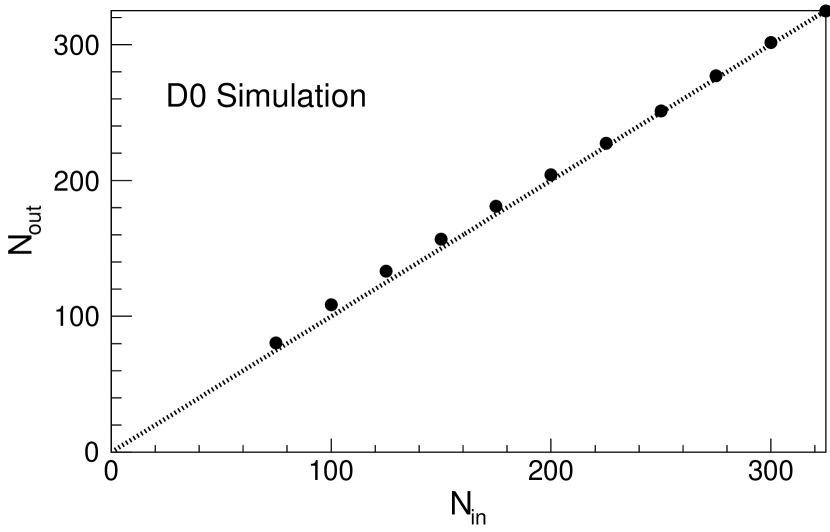
Figure 10: Results of the toy MC tests of the fitting procedure (black circles) used in the analysis of the semileptonic data with the cone cut. The number of fitted signal events are plotted vs fitted number of injected signal events. The dotted line shows $N_{\mathrm{in}}=N_{\mathrm{out}}$.

VII.4 Comparison with hadronic channel

The measured values of the mass, width, the number of signal events, and significance of the signal for the semileptonic channel and the hadronic channel Abazov et al. (2016) are given in Table 6. The mass and width of the $X^{\pm}(5568)$ for the semileptonic and hadronic channels are consistent taking into account the uncertainties. The observed yields are consistent with coming from a common particle given the number of $B_{s}^{0}$ events in the sample and the $B^{0}_{s}$ branching ratios.

Table 6: Fit results obtained in the semileptonic channel and in the hadronic channel (Ref. Abazov et al. (2016)). In the hadronic channel with no cone cut the mass and width of the $X^{\pm}(5568)$ were set to the values found with the cone cut. LEE - look elsewhere effect.

	Semileptonic		Hadronic (from Ref. Abazov et al. (2016))
	Cone cut	No cone cut	Cone cut	No cone cut
Fitted mass, MeV/$c^{2}$	$5566.4^{+3.4}_{-2.8}\ {}^{+1.5}_{-0.6}$	$5566.7^{+3.6}_{-3.4}\ {}^{+1.0}_{-1.0}$	$5567.8\pm 2.9^{+0.9}_{-1.9}$	5567.8
Fitted width, MeV/$c^{2}$	$2.0^{+9.5}_{-2.0}\ {}^{+2.8}_{-2.0}$	$6.0^{+9.5}_{-6.0}\ {}^{+1.9}_{-4.6}$	$21.9\pm 6.4^{+5.0}_{-2.5}$	21.9
Fitted number of signal events	$121^{+51}_{-34}\ {}^{+9}_{-28}$	$139^{+51}_{-63}\ {}^{+11}_{-32}$	$133\pm 31\pm 15$	$106\pm 23{\rm\thinspace(stat)}$
Local significance	$4.3\,\sigma$	$4.5\,\sigma$	$6.6\,\sigma$	$4.8\,\sigma$
Significance with systematics	$3.2\,\sigma$	$3.4\,\sigma$	$5.6\,\sigma$	…
Significance with LEE+systematics	…	…	$5.1\,\sigma$	$3.9\,\sigma$

VII.5 Cross-checks

As a cross-check the $B^{0}_{s}\pi^{\pm}$ mass-bin size is set to 5 MeV/$c^{2}$ and to 10 MeV/$c^{2}$ instead of 8 MeV/$c^{2}$, and the lower edge of the fitted mass range is shifted by 2, 3, 5, and 7 MeV/$c^{2}$. This leads to maximal variations in the mass of ${}^{+0.1}_{-0.6}$ MeV/$c^{2}$, in the width of ${}^{+1.7}_{-0.9}$ MeV/$c^{2}$ and in the number of signal events ${}^{+0}_{-9}$ which are small compared to the statistical and systematic uncertainties.

To test the stability of the results, alternative choices are made regarding the fit parameters. In the first, the background fit parameters are allowed to float. The resulting fit is consistent with the nominal fit and the $p$-value of the background-only fit is $1.7\times 10^{-4}$ corresponding to a statistical significance of 3.8 $\sigma$ (Table 7). The second cross-check fixes the mass and width of the $X^{\pm}(5568)$ to the values found in Ref. Abazov et al. (2016). Again, the resulting fit is consistent with the nominal fit with an increase in the number of signal events due to the increased width of the peak. The $p$-value of the background-only fit is $1.1\times 10^{-4}$ corresponding to a statistical significance of 3.9 $\sigma$ (Table 7). These cross-checks are also repeated without the cone cut (Table 7).

Table 7: Fit results for the semileptonic channel using parametrization (IV) with the nominal fit, with all parameters free and the mass and width fixed to those of the hadronic channel. Statistical uncertainties only.

	Nominal fit	All parameters free	Mass and width fixed to hadronic
Cone Cut
Fitted mass, MeV/$c^{2}$	$5566.4^{+3.4}_{-2.8}$	$5567.2\pm 2.9$	$5567.8$
Fitted width, MeV/$c^{2}$	$2.0^{+9.5}_{-2.0}$	$8.3\pm 11.0$	$21.9$
Fitted number of signal events	$121^{+51}_{-34}$	$181\pm 88$	$164\pm 44$
$\chi^{2}/$ndf	$34.9/(50-4)$	$30.9/(50-10)$	$38.0/(50-2)$
Local significance	$4.3\sigma$	$3.8\sigma$	$3.9\sigma$
No cone cut
Fitted mass, MeV/$c^{2}$	$5566.7^{+3.6}_{-3.4}$	$5566.6\pm 3.5$	$5567.8$
Fitted width, MeV/$c^{2}$	$6.0^{+9.5}_{-6.0}$	$8.4\pm 14.5$	$21.9$
Fitted number of signal events	$139^{+51}_{-63}$	$144\pm 101$	$168\pm 42$
$\chi^{2}/$ndf	$30.4/(50-4)$	$27.4/(50-10)$	$32.8/(50-2)$
Local significance	$4.5\sigma$	$4.4\sigma$	$4.2\sigma$

VIII Production ratio of $\bm{X^{\pm}(5568)}$ to $\bm{B_{s}^{0}}$

To calculate the production ratio of the $X^{\pm}(5568)$ to $B_{s}^{0}$, the number of the $B_{s}^{0}$-mesons needs to be estimated. The fitting of the $K^{+}K^{-}\pi^{\mp}$ mass distribution is described in Sec. IV. The number of $D_{s}^{\mp}$ mesons extracted from the fit and adjusted for the mass range $1.91<m(K^{+}K^{-}\pi^{\mp})<2.03$ MeV$/c^{2}$ is $N(D_{s}^{\mp})=6648\pm 127$ (see Fig. 2). The number of $\mu^{\pm}D_{s}^{\mp}$ events in the signal sample that are the result of a random combination of a promptly produced $D_{s}^{\mp}$ and a muon in the event is estimated using events where the muon and the $D_{s}^{\mp}$-meson have the same sign. The same sign data sample is analyzed using the same model as the opposite sign data with the means and widths of the Gaussians fixed to the values obtained from the opposite sign data. The number of events in the same-sign sample is $N(D_{s}^{\pm})=426\pm 61$. The mass distributions of the $K^{+}K^{-}\pi^{\mp}$ for opposite and same-sign data are shown in Fig. 2.

The number of $B^{0}_{s}$-meson decays in the semileptonic data is estimated by subtracting the contribution of the promptly produced $\mu^{\pm}D_{s}^{\mp}$ events from the overall $\mu^{\pm}D_{s}^{\mp}$ sample. A study of the MC background simulations shows that the purity of the resulting sample is $99.5^{+0.5}_{-1.0}\%$. We find $6222\pm 141$ $B^{0}_{s}$ events.

Combining these results and using the efficiency for the charged pion in the X(5568) decay (Sec. IV), we obtain a production ratio for the semileptonic data of

$$\rho {}=\frac{N_{\mathrm{sl}}(X^{\pm}(5568)\rightarrow B^{0}_{s}(\mathrm{sl})\pi^{\pm})}{N_{B^{0}_{s}}(\mathrm{sl})}$$

$${}=\left[7.3^{+2.8}_{-2.4}\thinspace{\rm(stat)}^{+0.6}_{-1.7}\thinspace{\rm(syst)}\right]\%,$$ (8)

for our fiducial selection (which includes the requirements $p_{T}(\mu^{\pm}D_{s}^{\mp})>10\,$GeV$/c^{2}$ and $4.5\,$GeV$/c^{2}\,<m(\mu^{\pm}D_{s}^{\mp})<m(B^{0}_{s})$), where $N_{\mathrm{sl}}(X^{\pm}(5568)\rightarrow B^{0}_{s}(\mathrm{sl})\pi^{\pm})$ is the number of $X^{\pm}(5568)$ decays to $B^{0}_{s}\pi^{\pm}$ and $N_{B^{0}_{s}}(\mathrm{sl})$ is the inclusive number of $B^{0}_{s}$ decays, both for semileptonic decays of the $B^{0}_{s}$. This result is similar to the ratio measured in the hadronic channel $\left[8.6\pm 1.9\thinspace{\rm(stat)}\pm 1.4\thinspace{\rm(syst)}\right]\%$ for $p_{T}(J/\psi\phi\pi^{\pm})>10\,$GeV$/c^{2}$ Abazov et al. (2016).

IX Combined Signal Extraction

We now proceed to fit the hadronic and semileptonic data sets simultaneously. The hadronic data set is the same as used in Ref. Abazov et al. (2016) except that the data are fitted in the mass range $5.506<m(B^{0}_{s}\pi^{\pm})<5.906$ GeV/$c^{2}$ instead of $5.500<m(B^{0}_{s}\pi^{\pm})<5.900$ GeV/$c^{2}$. The data selection and background modeling for the hadronic data set are described in detail in Ref. Abazov et al. (2016).

The fit function has the form

$$F_{\rm h}= {}f_{\rm h,sig}F_{\rm h,sig}(m,m_{X},\Gamma{{}_{X}})+f_{\rm h,bgr}F_{\rm h,bgr}(m),$$ (9)

$$F_{\rm sl}= {}f_{\rm sl,sig}F_{\rm sl,sig}(m,m_{X},\Gamma{{}_{X}})+f_{\rm sl,bgr}F_{\rm sl,bgr}(m)$$ (10)

where $f_{\rm h(sl),sig}$ and $f_{\rm h(sl),bgr}$ are normalization factors. The shape parameters in the background terms $F_{\rm h(sl),bgr}$ are fixed to the values obtained from fitting the respective background models for the hadronic (h) and semileptonic (sl) samples to Eq. (IV). The signal shape $F_{\rm h(sl),sig}$ is modeled by relativistic Breit-Wigner function convolved with a Gaussian detector resolution function that depends on the data sample. For the semileptonic sample the detector resolution is given by Eq. (5) and for the hadronic channel it is 3.85 MeV/$c^{2}$. For the data without the cone cut the combined data are fitted in the range $5.506<m(B^{0}_{s}\pi^{\pm})<5.706$ GeV/$c^{2}$ as the hadronic background is not well modeled for $m(B^{0}_{s}\pi^{\pm})>5.706$ GeV/$c^{2}$ Abazov et al. (2016). The same Breit-Wigner parameters $m_{X}$ and $\Gamma_{X}$ are used for the hadronic and semileptonic samples. In the fits shown in Fig. 11, the normalization parameters $f_{\rm h(sl),sig}$ and $f_{\rm h(sl),bgr}$ and the Breit-Wigner parameters $m_{X}$ and $\Gamma{{}_{X}}$ are allowed to vary. Since the fraction of $B^{0}_{s}$ events produced by the decay of the $X^{\pm}(5568)$ should be essentially the same in the hadronic and semileptonic channels the $X^{\pm}(5568)$ event yields ($N_{\mathrm{h}}$ and $N_{\mathrm{sl}}$) are constrained using the parameter

$$A_{\mathrm{sl,h}}=\frac{N_{\mathrm{sl}}-N_{\mathrm{h}}}{N_{\mathrm{sl}}+N_{\mathrm{h}}}$$ (11)

which is required to be consistent with the $B^{0}_{s}$-meson production rate in the hadronic and semileptonic channels

$$A_{\mathrm{sl,h}}(B^{0}_{s})=\frac{N_{B^{0}_{s}}(\mathrm{sl})-N_{B^{0}_{s}}(\mathrm{h})}{N_{B^{0}_{s}}(\mathrm{sl})+N_{B^{0}_{s}}(\mathrm{h})}=0.054\pm 0.020,$$ (12)

where $N_{B^{0}_{s}}(\mathrm{sl})=6222\pm 144$, $N_{B^{0}_{s}}(\mathrm{h})=5582\pm 100$ are the number of semileptonic and hadronic $B^{0}_{s}$ decays in the sample. A likelihood penalty of $0.5\left[(A_{\mathrm{sl,h}}-A_{\mathrm{sl,h}}(B^{0}_{s}))/\Delta A_{\mathrm{sl,h}}(B^{0}_{s})\right]^{2}$ is applied where $\Delta A_{\mathrm{sl,h}}(B^{0}_{s})=0.020$ is the uncertainty. This uncertainty includes the statistical uncertainty in the number of $B^{0}_{s}$ events and the uncertainties in the relative reconstruction efficiencies and acceptances between the hadronic and semileptonic data. A ratio has been chosen for the constraint as it is well behaved if either of the event yields ($N_{\mathrm{h}}$ and $N_{\mathrm{sl}}$) approaches zero.

The fit results are summarized in Table 8 and the correlations between the fit parameters are given in Table 9. The correlation of nearly one between $N_{X}(\mathrm{sl})$ and $N_{X}(\mathrm{had})$ is a result of the constraint on the event yields [Eq. (11)]. The local statistical significance of the signal is defined as $\sqrt{-2\,{\rm ln}({\cal{L}}_{0}/{\cal{L}}_{\mathrm{max}})}$, where ${\cal{L}}_{\mathrm{max}}$ and ${\cal{L}}_{0}$ are likelihood values at the best-fit signal yield and the signal yield fixed to zero obtained from a binned maximum-likelihood fit. For the cone cut the $p$-value of the fit to the data with the cone cut is $2.2\times 10^{-14}$ and the local statistical significance is 7.6 $\sigma$. The $p$-value without the cone cut is $8.2\times 10^{-9}$ and the local statistical significance is 5.8 $\sigma$.

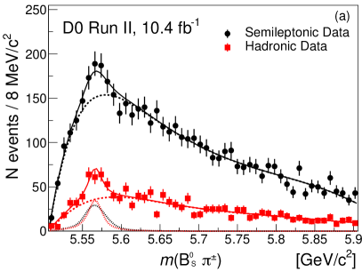
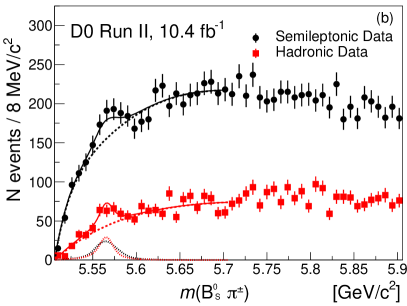
Figure 11: The $m(B^{0}_{s}\pi^{\pm})$ distribution for the hadronic (red squares) and semileptonic (black circles) data with the combined fitting function superimposed (a) with and (b) without the cone cut. (see text for details, the resulting fit parameters are given in Table 8). The background parametrization function is taken from Eq. (IV).

Table 8: Results for the combined fit to the hadronic and semileptonic data sets (see Fig. 11).

	Cone cut	No cone cut
Fitted mass, MeV/$c^{2}$	$5566.9^{+3.2}_{-3.1}\,\mbox{(stat)}^{+0.6}_{-1.2}\,\mbox{(syst)}$	$5565.8^{+4.2}_{-4.0}\,\mbox{(stat)}^{+1.3}_{-2.0}\,\mbox{(syst)}$
Fitted width, MeV/$c^{2}$	$18.6^{+7.9}_{-6.1}\,\mbox{(stat)}^{+3.5}_{-3.8}\,\mbox{(syst)}$	$16.3^{+9.8}_{-7.6}\,\mbox{(stat)}^{+4.2}_{-6.5}\,\mbox{(syst)}$
Fitted number of hadronic signal events	$131^{+37}_{-33}\,\mbox{(stat)}^{+15}_{-14}\,\mbox{(syst)}$	$99^{+40}_{-34}\,\mbox{(stat)}^{+18}_{-33}\,\mbox{(syst)}$
Fitted number of semileptonic signal events	$147^{+42}_{-37}\,\mbox{(stat)}^{+17}_{-16}\,\mbox{(syst)}$	$111.7^{+46}_{-39}\,\mbox{(stat)}^{+20}_{-38}\,\mbox{(syst)}$
$\chi^{2}/$ndf	$94.7/(100-6)$	$54.2/(50-6)$
$p$-value	$2.2\times 10^{-14}$	$1.9\times 10^{-8}$
Local significance	$7.6\,\sigma$	$5.6\,\sigma$
Significance with LEE	$6.9\,\sigma$	$5.0\,\sigma$
Significance with LEE+systematics	$6.7\,\sigma$	$4.7\,\sigma$

Table 9: Correlations between the parameters of the combined fit to the hadronic and semileptonic data sets (see Fig. 11). The yield in the semileptonic channel is $N_{X}(\mathrm{sl})$, the hadronic channel $N_{X}(\mathrm{h})$, while the fraction of background events is $f_{\rm sl,bgr}$ and $f_{\rm h,bgr}$ respectively.

Cone Cut
	Mass	Width	$N_{X}(\mathrm{sl})$	$N_{X}(\mathrm{h})$	$f_{\rm sl,bgr}$	$f_{\rm h,bgr}$
Mass	1	0.22	0.37	0.37	-0.06	-0.11
Width	0.22	1	0.58	0.59	-0.16	-0.29
$N_{X}(\mathrm{sl})$	0.37	0.58	1	0.98	-0.31	-0.44
$N_{X}(\mathrm{h})$	0.37	0.59	0.98	1	-0.30	-0.45
$f_{\rm sl,bgr}$	-0.06	-0.16	-0.31	-0.30	1	0.14
$f_{\rm h,bgr}$	-0.11	-0.29	-0.44	-0.45	0.14	1
No Cone Cut
	Mass	Width	$N_{X}(\mathrm{sl})$	$N_{X}(\mathrm{h})$	$f_{\rm sl,bgr}$	$f_{\rm h,bgr}$
Mass	1	0.38	0.49	0.49	-0.11	-0.17
Width	0.38	1	0.64	0.64	-0.18	-0.31
$N_{X}(\mathrm{sl})$	0.49	0.64	1	0.99	-0.33	-0.45
$N_{X}(\mathrm{h})$	0.49	0.64	0.99	1	-0.33	-0.46
$f_{\rm sl,bgr}$	-0.11	-0.18	-0.33	-0.33	1	0.15
$f_{\rm h,bgr}$	-0.17	-0.31	-0.45	-0.46	0.15	1

IX.1 Systematic uncertainties

The systematic uncertainties of the combined fit are given in Table 10. The uncertainty on (i) the background shape descriptions is evaluated by using the alternative paramaterizations of the background, Eqs. (2), (3) and the smoothed MC histogram independently for the semileptonic and the hadronic channels (16 different fits) and finding the maximal deviations from the nominal fit.

The effect of (ii) the MC weighting for the semileptonic background is estimated by creating 1000 background samples where the weights have been randomly varied based on the uncertainties in the weighting procedure and measuring the standard deviation and bias of the measured values.

The (iii) MC component of the background for the hadronic sample is made up of a mixture of two independent MC samples with different production properties (see Ref. Abazov et al. (2016)) and the systematic uncertainties due to this are found by varying the composition of this mixture and measuring the standard deviation and bias of the measured values. The (iv) size of the hadronic sidebands is varied using the maximal deviations from the nominal fit to estimate the systematic uncertainty.

The systematic uncertainty due to the (v) fraction of MC and SS data in the semileptonic sample, (vi) the MC and sideband data in the case of the hadronic, is varied independently between the two samples measuring the standard deviation and bias of the measured values. Since the background model for the semileptonic sample without the cone cut only uses the MC background simulation this uncertainty (v) does not apply.

All of the uncertainties due to the modeling of the background are assumed to be independent for the hadronic and semileptonic data samples.

The remaining uncertainties are measured by finding the maximal deviations from the nominal fit for (vii) varying the energy scale in the semileptonic and hadronic MC data samples by $\pm$1 MeV/$c^{2}$ in both samples simultaneously; (viii) varying the nominal mass resolution of 3.85 MeV/$c^{2}$ for the D0 detector by $\pm$1 MeV/$c^{2}$ and $+2$ MeV/$c^{2}$ in both the hadronic and semileptonic data samples simultaneously; (ix) varying the resolution of the $X^{\pm}(5568)$ peak in the semileptonic channel either by $\pm$1 MeV/$c^{2}$ around the mean value given by Eq. (5) or by using a constant resolution of 11.1 MeV/$c^{2}$ for the semileptonic data while the mass resolution in the hadronic channel remains at 3.85 MeV/$c^{2}$; (x) using a P-wave relativistic Breit-Wigner function for both data sets; (xi) setting the shift of the fitted mass peak in the semileptonic data with respect to the hadronic data due to the missing neutrino to $\pm$1 MeV/$c^{2}$; and (xii) varying the constraint on the relative number of signal events in hadronic and semileptonic channels (Eq. (11)) between 0.034 and 0.074. The correlation of each of the sources of systematic uncertainty between the hadronic and semileptonic data sets is indicated in Table 10. The uncertainties are added in quadrature separately for positive and negative values to obtain the total systematic uncertainties for each measured parameter. The results including systematic uncertainties are given in Table 8.

Table 10: Systematic uncertainties of the combined fit for the $X^{\pm}(5568)$ state mass, width and the event yields. Each uncertainty is either correlated or uncorrelated between the hadronic and semileptonic data sets.

Source	Sample	Mass, MeV/$c^{2}$	Width, MeV/$c^{2}$	Event yields, events
				hadronic	semileptonic
Cone Cut
(i) Background shape description	Both	$+0.3$  ; $-0.6$	$+1.9$  ; $-0.0$	$+0.0$  ; $-6.6$	$+0.0$  ; $-7.8$
(ii) SL background reweighting	Semileptonic	$+0.1$  ; $-0.2$	$+0.2$  ; $-0.2$	$+2.5$  ; $-3.3$	$+2.9$  ; $-3.9$
(iii) Hadronic MC samples	Hadronic	$+0.3$  ; $-0.2$	$+1.2$  ; $-0.4$	$+7.0$  ; $-2.5$	$+7.8$  ; $-2.8$
(iv) Hadronic sidebands	Hadronic	$+0.1$  ; $-0.1$	$+0.5$  ; $-1.3$	$+2.3$  ; $-9.3$	$+2.5$  ; $-10.2$
(v) SL MC/Data ratio	Semileptonic	$+0.0$  ; $-0.1$	$+0.1$  ; $-0.1$	$+1.0$  ; $-1.2$	$+1.1$  ; $-1.4$
(vi) Hadronic MC simulation/data ratio	Hadronic	$+0.0$  ; $-0.0$	$+0.2$  ; $-0.2$	$+1.0$  ; $-1.1$	$+1.1$  ; $-1.2$
(vii) $B_{s}^{0}$ mass scale, MC simulation and data	Both	$+0.2$  ; $-0.2$	$+0.8$  ; $-0.8$	$+3.7$  ; $-4.3$	$+4.1$  ; $-4.7$
(viii) Detector resolution	Both	$+0.1$  ; $-0.3$	$+1.3$  ; $-3.4$	$+1.4$  ; $-3.8$	$+1.6$  ; $-4.2$
(ix) Missing neutrino effect	Semileptonic	$+0.1$  ; $-0.1$	$+0.1$  ; $-0.0$	$+0.5$  ; $-0.1$	$+0.0$  ; $-0.4$
(x) P-wave Breit-Wigner	Both	$+0.0$  ; $-0.0$	$+2.1$  ; $-0.0$	$+11.7$  ; $-0.0$	$+13.0$  ; $-0.0$
(xi) Mass offset	Both	$+0.3$  ; $-0.3$	$+0.1$  ; $-0.0$	$+0.2$  ; $-0.4$	$+0.3$  ; $-0.4$
(xii) Production fraction	Both	$+0.0$  ; $-0.0$	$+0.1$  ; $-0.1$	$+1.4$  ; $-1.6$	$+4.2$  ; $-4.2$
Total		$+0.6$  ; $-1.2$	$+3.5$  ; $-3.8$	$+14.7$  ; $-13.6$	$+16.9$  ; $-15.8$
No Cone Cut
(i) Background shape description	Both	$+1.1$  ; $-1.9$	$+1.4$  ; $-5.1$	$+7.6$  ; $-32.8$	$+8.4$  ; $-37.1$
(ii) SL background reweighting	Semileptonic	$+0.1$  ; $-0.0$	$+0.1$  ; $-0.3$	$+1.8$  ; $-1.1$	$+2.0$  ; $-1.4$
(iii) Hadronic MC samples	Hadronic	$+0.3$ …  ; $-0.0$	$+1.1$  ; $-0.0$	$+7.2$  ; $-0.0$	$+7.9$  ; $-0.0$
(iv) Hadronic Sidebands	Hadronic	$+0.3$  ; $-0.1$	$+0.2$  ; $-0.6$	$+4.5$  ; $-3.7$	$+4.9$  ; $-4.2$
(v) SL MC simulation/data ratio	Not applicable	…  ; …	…  ; …	…  ; …	…  ; …
(v) Hadronic MC simulation/data ratio	Hadronic	$+0.1$  ; $-0.0$	$+0.5$  ; $-0.0$	$+7.4$  ; $-0.1$	$+8.1$  ; $-0.2$
(vii) $B_{s}^{0}$ mass scale, MC simulation and data	Both	$+0.1$  ; $-0.1$	$+0.9$  ; $-0.2$	$+5.1$  ; $-0.0$	$+5.6$  ; $-0.0$
(viii) Detector resolution	Both	$+0.1$  ; $-0.2$	$+1.6$  ; $-3.9$	$+1.5$  ; $-3.5$	$+1.6$  ; $-4.0$
(ix) Missing neutrino effect	Semileptonic	$+0.2$  ; $-0.1$	$+0.1$  ; $-0.1$	$+0.4$  ; $-0.0$	$+0.1$  ; $-0.3$
(x) P-wave Breit-Wigner	Both	$+0.0$  ; $-0.6$	$+3.3$  ; $-0.0$	$+10.7$  ; $-0.0$	$+11.8$  ; $-0.0$
(xi) Mass offset	Both	$+0.4$  ; $-0.4$	$+0.2$  ; $-0.2$	$+0.0$  ; $-0.0$	$+0.0$  ; $-0.1$
(xii) Production fraction	Both	$+0.0$  ; $-0.0$	$+0.1$  ; $-0.1$	$+0.8$  ; $-0.8$	$+3.5$  ; $-3.6$
Total		$+1.3$  ; $-2.0$	$+4.2$  ; $-6.5$	$+18.2$  ; $-33.2$	$+20.3$  ; $-37.8$

IX.2 Significance

The look-elsewhere effect (LEE) is determined using the approach proposed in Ref. Gross and Vitells (2010). We have generated 250,000 simulated background distributions with no signal, both with and without the cone cut. These distributions are fit using the same procedure as the data. The mass parameter of the relativistic Breit-Wigner is constrained to be between 5506 to 5675 MeV/$c^{2}$ (the sum of the mass of the $B^{0}_{d}$ and $K^{\pm}$) with a starting value of $m_{X}=5600$ MeV/$c^{2}$. The width of the signal is allowed to vary between 0.1 and 60 MeV/$c^{2}$ with a starting value of $\Gamma_{X}=21$ MeV/$c^{2}$. The maximum local statistical significance for each distribution is calculated. The resulting distribution of the local significance is fitted with the function

$$f_{\mathrm{loc}}=N_{\mathrm{trials}}\left[\chi^{2}(2)+P_{1}\chi^{2}(3)\right],$$ (13)

where $N_{\mathrm{trials}}$ is the number of generated distributions, $P_{1}$ is a free parameter and $\chi^{2}(n)$ is the $\chi^{2}$ cumulative distribution function for $n$ degrees of freedom. We have used $n=2$ and 3 as we are fitting two spectra simultaneously. The resulting function is integrated above the measured local significance to determine the global significance (Table 8). The significance, not including the systematic uncertainty, of the observed signal accounting for the LEE and with the cone cut applied is 6.9 $\sigma$ ($p$-value = $4.1\times 10^{-12}$). The significance of the signal without the cone cut is 5.0 $\sigma$ ($p$-value = $4.1\times 10^{-7}$). The effect of choosing the function in Eq. (13) is studied by modifying it to $f_{\mathrm{loc}}=N_{\mathrm{trials}}\left[\chi^{2}(2)+P_{1}\chi^{2}(4)\right]$ and $f_{\mathrm{loc}}=N_{\mathrm{trials}}\left[\chi^{2}(2)+P_{1}\chi^{2}(3)+P_{2}\chi^{2}(4)\right]$ with no significant change to the significance being observed. The look-elsewhere effect on the signal significance is checked with a method described in Ref. Gross and Vitells (2010) that relates the tail probability with the number of “upcrossing” at a small reference level. Five hundred simulated background spectra are generated. Each of these 500 distributions is fitted with the background plus signal function with different initial masses from 5506 to 5675 MeV/$c^{2}$ in 5 MeV/$c^{2}$ steps along with a background-only fit. The significance is plotted for each of the mass points and the number of upcrossings (each time the significance crosses a small reference value) is measured. The mean number of upcrossings for a reference level of 0.5 is determined and the global significance is calculated. The resulting significance is consistent with the method described above.

The systematic uncertainties are treated as nuisance parameters to construct a prior predictive model Patrignani et al. (2016); Giunti (1999) of our test statistic. When the systematic uncertainties are included, the significance of the observed signal with the cone cut applied for the combined fit is reduced to 6.7 $\sigma$ ($p$-value = $1.5\times 10^{-11}$) and the significance of the signal without the cone cut is 4.7 $\sigma$ ($p$-value = $2.0\times 10^{-6}$).

IX.3 Closure tests

To test the sensitivity and accuracy of the fitting procedure for the combined signal extraction we repeat the closure tests carried out in Sec. VII.3 with the following modifications. The size of the associated hadronic signal is set using Eqs. (11) and (12). The appropriate detector resolution is used, Eq. (5) for the semileptonic sample and 3.85 MeV/$c^{2}$ for the hadronic sample. For each trial the fitting procedure is performed to obtain the mass and width and the number of semileptonic and hadronic signal events. The results of each set of trials is fitted with a Gaussian to determine the mean and the uncertainty in the number of signal events, the mass and the width (see Table 11). The number of fitted signal events vs. the number of injected signal events for the semileptonic and hadronic samples is plotted in Fig. 12. These results show excellent agreement between the input and fit parameters.

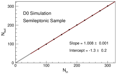
(a) Semileptonic Sample

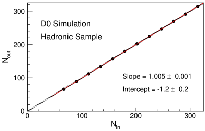
(b) Hadronic Sample

Figure 12: Results of the toy MC tests of the combined sample fitting procedure (black circles) used in the analysis with the cone cut. The number of fitted signal events are plotted vs fitted number of injected signal events for the (a) semileptonic and (b) hadronic samples. The dotted line shows $N_{\mathrm{in}}=N_{\mathrm{out}}$ and the red line shows the fit to a line.

Table 11: Mean values and uncertainties for fitted number of events, mass and width from Gaussian fits to corresponding distributions from 10,000 trials with the cone cut. Also given is the expected statistical uncertainties on the fitted number of events, $\Delta$($N_{\mathrm{fit}}$), and the expected uncertainties on the measurement of the width, $\Delta(\Gamma_{X})$ MeV/$c^{2}$. A range of signals with 75, 100, 125, 150, 175 and 200 signal events, mass $m_{x}=5568.3$ MeV$/c^{2}$ and width $\Gamma_{X}=21.9$ MeV$/c^{2}$ have been simulated. Background parametrization Eq. (IV) is used.

Semileptonic channel			Hadronic channel			$m_{X}$	$\Gamma_{X}$	$\Delta(\Gamma_{X})$
$N_{\mathrm{in}}(\mathrm{sl})$	$N_{\mathrm{fit}}(\mathrm{sl})$	$\Delta$($N_{\mathrm{fit}}(\mathrm{sl})$)	$N_{\mathrm{in}}(\mathrm{h})$	$N_{\mathrm{fit}}(\mathrm{h})$	$\Delta$($N_{\mathrm{fit}}(\mathrm{h})$)	MeV/$c^{2}$	MeV/$c^{2}$	MeV/$c^{2}$
75	$73.8\pm 0.3$	25.7	67.3	$66.0\pm 0.2$	23.0	$5569.0\pm 0.076$	19.3	10.9
100	$99.1\pm 0.3$	26.3	89.8	$88.7\pm 0.2$	23.6	$5568.4\pm 0.042$	20.8	9.2
125	$124.9\pm 0.3$	26.8	112.2	$111.7\pm 0.2$	24.0	$5568.4\pm 0.032$	21.5	7.8
150	$149.6\pm 0.3$	26.5	134.6	$133.8\pm 0.2$	23.6	$5568.4\pm 0.027$	21.9	6.8
175	$175.9\pm 0.3$	27.2	157.1	$157.3\pm 0.2$	24.3	$5568.4\pm 0.023$	22.3	6.0
200	$200.8\pm 0.3$	27.2	179.5	$179.6\pm 0.2$	24.2	$5568.4\pm 0.021$	22.4	5.4

IX.4 Cross-checks

To test the stability of the results, alternative choices are made regarding the fit parameters (see Table 12).

When no constraint is placed on the ratio of the event yields in the hadronic and semileptonic channels, Eq. (11), the results are entirely consistent with the fit with the constraint.

We have also carried out a fit in which two of the systematic effects are treated as nuisance parameters in the fit. We allow a mass shift, $\Delta m$, between the hadronic and semileptonic data with a likelihood penalty of $0.5(\Delta m/1\,\mathrm{MeV}/c^{2})^{2}$. We also allow the overall resolution of the semileptonic signal to vary by $\Delta\sigma_{\mathrm{SL}}$ with a likelihood penalty of $0.5(\Delta\sigma_{\mathrm{SL}}/1\,\mathrm{MeV}/c^{2})^{2}$. The resultant fit produces a mass, width and event yields that are consistent with the default fit and shifts of $\Delta m=(0.0\pm 1.4)$ MeV/$c^{2}$ and $\Delta\sigma_{\mathrm{SL}}=(-0.1\pm 1.4)$ MeV/$c^{2}$.

The significance of a nonzero width is determined by fitting the data with the width set to zero and comparing it with the fit with no constraint on the width (Table 12). Using the data with the cone cut the $p$-value of the width being consistent with zero is $5.4\times 10^{-6}$, and the statistical significance is 4.5 $\sigma$. The significance without the cone cut is 3.3 $\sigma$ ($p$-value = $1.1\times 10^{-3}$).

Table 12: Various cross checks for the combined fit of the hadronic and semileptonic data sets.

	Default fit	No production constraint	Nuisance parameter	Zero width
Cone Cut
Fitted mass, MeV/$c^{2}$	$5566.9^{+3.2}_{-3.1}$	$5566.8^{+3.2}_{-3.1}$	$5567.4^{+3.2}_{-3.4}$	$5569.9^{+1.3}_{-1.3}$
Fitted width, MeV/$c^{2}$	$18.6^{+7.9}_{-6.1}$	$18.3^{+8.0}_{-6.2}$	$21.7^{+7.3}_{-5.5}$	$0$
Fitted number of hadronic signal events	$131^{+37}_{-33}$	$127^{+34}_{-29}$	$134^{+37}_{-33}$	$60^{+17}_{-16}$
Fitted number of semileptonic signal events	$147^{+42}_{-37}$	$159^{+66}_{-59}$	$151^{+41}_{-37}$	$68^{+19}_{-18}$
$\chi^{2}/$ndf	$94.7/(100-6)$	$94.5/(100-6)$	$94.8/(100-8)$	$115.4/(100-7)$
$p$-value	$2.2\times 10^{-14}$	$2.0\times 10^{-14}$	$2.4\times 10^{-14}$	$8.5\times 10^{-10}$
Local significance	$7.6\,\sigma$	$7.7\,\sigma$	$7.6\,\sigma$	$6.1\,\sigma$
No cone cut
Fitted mass, MeV/$c^{2}$	$5565.8^{+4.2}_{-4.0}$	$5565.8^{+4.1}_{-3.9}$	$5566.3^{+4.4}_{-4.6}$	$5569.7^{+1.6}_{-1.9}$
Fitted width, MeV/$c^{2}$	$16.3^{+9.8}_{-7.6}$	$15.0^{+9.6}_{-7.8}$	$20.0^{+9.1}_{-9.4}$	$0$
Fitted number of hadronic signal events	$99^{+40}_{-34}$	$84^{+43}_{-35}$	$103^{+40}_{-37}$	$48^{+17}_{-16}$
Fitted number of semileptonic signal events	$112^{+46}_{-39}$	$151^{+72}_{-61}$	$115^{+45}_{-42}$	$54^{+20}_{-18}$
$\chi^{2}/$ndf	$54.2/(50-6)$	$52.5/(50-6)$	$54.8/(50-8)$	$101.3/(50-7)$
$p$-value	$1.9\times 10^{-8}$	$8.2\times 10^{-9}$	$2.7\times 10^{-8}$	$5.1\times 10^{-6}$
Local significance	$5.6\,\sigma$	$5.8\,\sigma$	$5.6\,\sigma$	$4.6\,\sigma$

X Conclusions

We have presented the results of a search for the $X^{\pm}(5568)\to B^{0}_{s}\pi^{\pm}$ with semileptonic decays of the $B_{s}^{0}$ meson. The $X^{\pm}(5568)\to B_{s}^{0}\pi^{\pm}$ state reported in the case that $B^{0}_{s}\to J/\psi\phi$ Abazov et al. (2016) is confirmed for the case that $B_{s}^{0}\rightarrow\mu^{\mp}D_{s}^{\pm}\,\mathrm{X}$, $D_{s}^{\pm}\rightarrow\phi\pi^{\pm}$. The analyses of the hadronic and semileptonic data give similar measurements of the mass, width and production ratio of $X^{\pm}(5568)$ to a $B^{0}_{s}$ meson. The mass and width of this state are measured using a combined fit of both data sets with the cone cut, yielding $m=5566.9^{+3.2}_{-3.1}\thinspace{\rm(stat)}^{+0.6}_{-1.2}{\rm\thinspace(syst)}$ MeV/$c^{2}$, $\Gamma=18.6^{+7.9}_{-6.1}{\rm\thinspace(stat)}^{+3.5}_{-3.8}{\rm\thinspace(syst)}$ MeV/$c^{2}$. The p-value for the null signal hypothesis to represent the data is $1.5\times 10^{-11}$ (6.7$\,\sigma$).

XI Acknowledgements

This document was prepared by the D0 collaboration using the resources of the Fermi National Accelerator Laboratory (Fermilab), a U.S. Department of Energy, Office of Science, HEP User Facility. Fermilab is managed by Fermi Research Alliance, LLC (FRA), acting under Contract No. DE-AC02-07CH11359.

We thank the staffs at Fermilab and collaborating institutions, and acknowledge support from the Department of Energy and National Science Foundation (United States of America); Alternative Energies and Atomic Energy Commission and National Center for Scientific Research/National Institute of Nuclear and Particle Physics (France); Ministry of Education and Science of the Russian Federation, National Research Center “Kurchatov Institute” of the Russian Federation, and Russian Foundation for Basic Research (Russia); National Council for the Development of Science and Technology and Carlos Chagas Filho Foundation for the Support of Research in the State of Rio de Janeiro (Brazil); Department of Atomic Energy and Department of Science and Technology (India); Administrative Department of Science, Technology and Innovation (Colombia); National Council of Science and Technology (Mexico); National Research Foundation of Korea (Korea); Foundation for Fundamental Research on Matter (The Netherlands); Science and Technology Facilities Council and The Royal Society (United Kingdom); Ministry of Education, Youth and Sports (Czech Republic); Bundesministerium für Bildung und Forschung (Federal Ministry of Education and Research) and Deutsche Forschungsgemeinschaft (German Research Foundation) (Germany); Science Foundation Ireland (Ireland); Swedish Research Council (Sweden); China Academy of Sciences and National Natural Science Foundation of China (China); and Ministry of Education and Science of Ukraine (Ukraine).