Controlled trapping of single particle states on a periodic substrate by deterministic stubbing

Abstract

A periodic array of atomic sites, described within a tight binding formalism is shown to be capable of trapping electronic states as it grows in size and gets stubbed by an ‘atom’ or an ‘atomic’ clusters from a side in a deterministic way. We prescribe a method based on a real space renormalization group method, that unravels a subtle correlation between the positions of the side coupled atoms and the energy eigenvalues for which the incoming particle finally gets trapped. We discuss how, in such conditions, the periodic backbone gets transformed into an array of infinite quantum wells in the thermodynamic limit. We present a case here, where the wells have a hierarchically distribution of widths, hosing standing wave solutions in the thermodynamic limit.

I Introduction

The ubiquitous and unavoidable phenomenon of Anderson localization in disordered systems has been alive for almost six decades now anderson ; abrahams ; kramer , with variations and surprises that have gone well beyond the realm of electronic systems, and incorporate phonons monthus , magnons lyo , photonics john ; yablono and matter waves  roati in recent times. The pivotal result in this field is that, all the single particle eigenfunctions remain exponentially localized in one and in two dimensions, irrespective of the strength of disorder. In three dimensions however, there remains a possibility of observing mobility edges separating the localized states from the extended, current carrying ones.

With the emergence of nano-fabrication techniques, interesting variants of Anderson localization can be put to test. One non-trivial variation of incorporating disorder is by coupling, from a side, a group of atoms that functionalize an otherwise periodically ordered backbone, which might mimic a quantum wire orellana ; grosso . The coupling of discrete structures from a side initiates the incorporation of bound states in the continuum, giving rise to the interesting Fano line shapes in the transmission spectrum mirosh ; sergej , and even in the density of states of the backbone-adatom system.

In spite of the existing canonical cases of disorder induced localization in one dimensional systems, short range positional correlation has been shown to lead to unscattered, extended single particle states for special values of electron energies dunlap . The positional correlations among the constituents were exploited for quasiperiodically ordered one dimensional chains, leading to the observation of an infinite number of such unscattered eigenstates, obtained by exploiting the inherent self similarity of the concerned lattices ac1 ; ac2 . Recently, the minimal quasi-one dimensionality introduced by the side coupled atomic clusters, in various topological shapes, have been shown to lead even to a complete delocalization of the electronic states, over the entire (or, almost the entire) range of the permissible spectrum atanu ; biplab1 ; biplab2 .

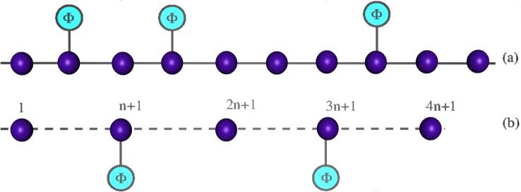
Figure 1: (Color online). (a) A periodic chain of atomic sites, acting as the ‘backbone’ is stubbed by single level quantum dots at positions following a middle third Cantor sequence. (b) The dots are now side coupled to a renormalized version of the same lattice that has been obtained by decimating out a set of $n$ sites uniformly.

In this communication, our focus is on a different aspect. We consider a periodically ordered linear lattice, where all the single particle states are Bloch functions, extended and transparent, over a range of energy $[\epsilon-2t,\epsilon+2t]$, when we use a tight binding Hamiltonian with nearest neighbor hopping approximation to describe the lattice. In the standard language, $\epsilon$ and $t$ are referred to as the ‘on site’ potential and the nearest neighbor ‘hopping integral’ respectively. This lattice is then ’stubbed’ deterministically, at predictably selected set of sites, infinite in number, when the periodic backbone is also infinite in size. The side coupled entities can be single level ‘quantum dot’s (QD) or quantum rings threaded by a magnetic flux. Both the ‘dot’ and the ‘ring’ are modelled in the same tight binding formalism.

We show that, for a specified, completely deterministic set of energy eigenvalues, an electron travelling in such a stubbed lattice will eventually get trapped in quantum wells, with a hierarchical distribution of widths. The values of the trapping energy can be engineered at will, covering for example, the entire range for which the periodic backbone supported extended, transparent Bloch states. This can be accomplished by stubbing the backbone from a side with the QD’s (or rings) at vertices farther and farther apart in the parent chain. The locations of such vertices can be easily determined via a real space renormalization group (RSRG) decimation technique. With increasing inter-stub separations, the distribution of the ‘trapping energy’ eigenvalues gets more and more densely populated, being driven towards a continuous distribution in the thermodynamic limit. Even with a finite value of the potential offered by the defected sites, the lattice, in the thermodynamic limit, turns out to be consisting of an infinite array of quantum wells with the heights of the walls growing finally to infinity, following a power law, as revealed only by repeated length scaling of the initial stubbed backbone.

In what follows we describe the method and the central results. In section I we describe the Hamiltonian and the basic scheme of the work, describing in details the RSRG scheme. Section II discusses the one dimensional periodic chain stubbed from a side with geometric structures. Two cases are discussed. First, we explain the way to trap electrons over the entire range of eigenvalues of a linear periodic chain. This is done using a single level QD. In the second example, we show how to control the energy values at will by fixing quantum rings threaded by a magnetic flux at a set of sites throughout the infinite backbone. Section III discusses the results, and in section IV we discuss the basic principle of trapping light waves using an elementary model for monomode wave guides which is stubbed at suitable points. In section V we draw conclusions.

The model and the preliminaries. – We describe our system of a linear periodic lattice in the tight binding formalism, using the Hamiltonian for spinless, non-interacting electrons with nearest neighbor interaction:

$$H=\epsilon\sum_{j}|j\rangle\langle j|+t\sum_{<jk>}(|j\rangle\langle k|+h.c.)$$ (1)

where, $\epsilon$ and $t$ are the constant on-site potential and uniform nearest neighbor hopping integral respectively. The index $k$ thus has values $j\pm 1$. The Schrödinger equation for this lattice is written in an equivalent form of a difference equation for every site $j$ as,

$$(E-\epsilon)\psi_{j}=t(\psi_{j-1}+\psi_{j+1})$$ (2)

We now digress a bit to remind ourselves an interesting property of a one dimensional fractal, viz, a middle third Cantor sequence. The Cantor array is sequentially built up using two characters, say $L$ and $S$. We take them to represent two kinds of ‘bonds’ in a linear atomic chain. The growth rule of the Cantor sequence we discuss here is, $L\rightarrow LSL$ and $S\rightarrow SSS$, beginning with an $L$ bond (the first generation). The first three generations will read, $G_{1}=L$, $G_{2}=LSLSSSLSL$ and $G_{3}=LSLS^{3}LSLS^{9}LSLS^{3}LSL$, and one can figure out the shape of the lattice at any $n$-th stage, $G_{n}$. A tight binding description of electronic states using the Hamiltonian in Eq. (1) for such a lattice requires the identification of three different kinds of on-site potentials, namely, $\epsilon_{\alpha}$, $\epsilon_{\beta}$ and $\epsilon_{\gamma}$, for the atomic sites residing between the pair of bonds $L-L$, $L-S$ and $S-L$ respectively. The nearest neighbor hopping integrals are named $t_{L}$ or $t_{S}$ depending on the bond $L$ or $S$ the electron hops across.

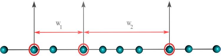
Figure 2: (Color online). Schematic representation of an $n$ times renormalized Cantor lattice with $E=\epsilon_{\alpha}=\epsilon_{\gamma}\neq\epsilon_{\beta}$ and $t_{L}=t_{S}$. The renormalized $\beta$ sites (encircled in red) erect infinitely large effective value of the on-site potential as $n\rightarrow\infty$. The widths $W_{1}$, $W_{2}$ follow a hierarchical distribution, dictated by the Cantor sequence.

Because of the inherent self similar hierarchical way the lattice builds up, it is easy to renormalize any $n$-th generation back to the $n-1$th generation by reversing the inflation rule. The process of renormalization leads to the recursion relations for the potential and the hopping terms, that are given by sheelan ,

$$\epsilon_{\alpha,n} = \epsilon_{\alpha,n-1}+\frac{2t_{S,n-1}^{2}(E-\epsilon_{\alpha,n-1})}{\Delta_{1,n-1}}$$

$$\epsilon_{\beta,n} = \epsilon_{\beta,n-1}+\frac{t_{L,n-1}^{2}(E-\epsilon_{\beta,n-1})}{\Delta_{2,n-1}}+\frac{t_{S,n-1}^{2}(E-\epsilon_{\alpha,n-1})}{\Delta_{1,n-1}}$$

$$\epsilon_{\gamma,n} = \epsilon_{\gamma,n-1}+\frac{t_{L,n-1}^{2}(E-\epsilon_{\gamma,n-1})}{\Delta_{2,n-1}}+\frac{t_{S,n-1}^{2}(E-\epsilon_{\alpha,n-1})}{\Delta_{1,n-1}}$$

$$t_{L,n} = \frac{t_{L,n-1}^{2}t_{S,n-1}}{\Delta_{2,n-1}}$$

$$t_{S,n} = \frac{t_{S,n-1}^{3}}{\Delta_{1,n-1}}$$ (3)

where, $\Delta_{1,n}=(E-\epsilon_{\alpha,n})^{2}-t_{S,n}^{2}$ and, $\Delta_{2,n}=(E-\epsilon_{\beta,n})(E-\epsilon_{\gamma,n})-t_{S,n}^{2}$.

An interesting observation can be made using the set of Eq. (3). If we set $E=\epsilon_{\alpha}=\epsilon_{\gamma}\neq\epsilon_{\beta}$, and $t_{L}=t_{S}$ at the bare length scale, then with successive renormalization, the parameters evolve as, $\epsilon_{\alpha,n+1}=\epsilon_{\gamma,n+1}$, $\epsilon_{\beta,n+1}=2\epsilon_{\beta,n}-2$, and $t_{L,n+1}=t_{S,n+1}=-t_{L,n}=-t_{S,n}$ for $n\geq 0$. Two important aspects are to be noted here. First, we observe that the effective on-site potential at the $\beta$ sites grows with every iteration, and second, the hopping integrals remain equal in magnitude at every stage of RSRG operation, and get locked into a two cycle fixed point. This implies that, in the limit $n\rightarrow\infty$, which essentially means that we are looking at the lattice in its thermodynamic limit, the incoming electron (with energy $E=\epsilon_{\alpha}$) will see an array of infinite potential wells of a hierarchy of widths. Following Lindquist and Riklund lind , it can be understood that, in the limit of infinite well depths (achieved only when the lattice extends to infinity), standing waves are formed in the quantum wells trapping the electron. As observed in the literature lind , the envelope of the standing well in a quantum well comprising $N$ discrete sites is given by,

$$\psi_{m,n}=\sqrt{\frac{2}{N+1}}\sin\left(\frac{mn\pi}{N+1}\right)$$ (4)

We exploit this phenomenon to trap an electron travelling in linear periodic lattice, as explained below.

Trapping an electron on a linear ordered chain. – Blocking propagation over the energy range $[\epsilon-2t,\epsilon+2t]$. –

Let us refer to Fig.1. The periodic chain is depicted with black circles at the atomic sites. We ‘artificially’ assign the bonds the ‘names’ $L$ and $S$ from the left following the growth rule of the Cantor sequence as discussed in the last section. Then it is easy to identify the $\beta$ sites, as well as the $\alpha$ and the $\gamma$ ones. We must appreciate that this design is artificial and the ‘pure’ character of the host lattice doesn’t change in terms of its energy spectrum and the nature of the eigenfunctions. Next we attach, in the simplest case, an atom, mimicking a single level QD from one side (cyan circles) to each ‘$\beta$’ site. The QD, assigned the same on-site potential $\epsilon$ as the backbone, is coupled to the backbone through a tunnel hopping $\lambda$. This immediately makes the lattice resemble a Cantor chain in the site model, where we automatically ensure $\epsilon_{\alpha}=\epsilon_{\gamma}\neq\epsilon_{\beta}$ and $t_{L}=t_{S}$ at the bare length scale. We then iterate the recursion relations Eq. (3) with the initial values, $\epsilon_{\alpha}=\epsilon_{\gamma}=\epsilon$, $\epsilon_{\beta}=\lambda^{2}/(E-\epsilon)$, which is obtained by renormalizing the self energy at the $\beta$ site (by ‘folding’ back the adatom into it), and $t_{L}=t_{S}=t$.

We have assigned a constant value of the on-site potential, viz. $\epsilon$ to the backbone, and the same potential is assigned to the attached QD as well. Next, the energy is chosen to be $E=\epsilon_{\alpha}=\epsilon_{\gamma}=\epsilon$. The recursion relations evolve and with every iteration the effective, renormalized potential at the $\beta$ site increases following the rule $\epsilon_{\beta,n}=2\epsilon_{\beta,n-1}-2$, while the renormalized nearest neighbor hopping integrals get locked into a two cycle fixed point, implying that the wave functions at two nearest neighbors at any scale of length has non-zero overlap. This implies that the states, in the limit $n\rightarrow\infty$, are standing waves, trapping the electron with energy $E=\epsilon$ eventually, in the thermodynamic limit. The energy $E=\epsilon$ is the center of the band of the ordered substrate, without stubs.

The scheme outlined above gives us an opportunity to engineer the energy values at which we can trap the propagating electron at will. To achieve this goal, we renormalize the parent lattice (without adatoms) first, by sequentially decimating clusters of $n$ atoms. This leads to the renormalization of the on-site potential and the nearest neighbor hopping integrals to,

$$\epsilon_{eff}(E) = \epsilon+\frac{2tU_{n-1}(x)}{U_{n}(x)}$$

$$t_{eff}(E) = \frac{t}{U_{n}(x)}$$ (5)

It is now necessary to identify the artificial $\beta$ sites on this renormalized lattice and attach the single level QD to them, to make the renormalized system resemble again a Cantor sequence of sites, at a larger scale of length and with energy dependent on-site potentials and hopping integrals. If we map back to the original scale of length then it is obvious that now the stubs are places farther apart. The final effective potential at the $\beta$ site on this rescaled version of the backbone is, $\epsilon_{\beta}^{eff}=\epsilon_{eff}(E)+\lambda^{2}/(E-\epsilon)$. The set of parameters with which the recursion relations Eq. (3) now begin to iterate is, $\epsilon_{\alpha,0}=\epsilon_{\gamma,0}=\epsilon+2tU_{n-1}(x)/U_{n}(x)$, $\epsilon_{\beta,0}=\epsilon+2tU_{n-1}(x)/U_{n}(x)+\lambda^{2}/(E-\epsilon)$, $t_{L,0}=t_{S,0}=t/U_{n}(x)$. Here, $x=(E-\epsilon)/2t$.

We now need to look for the solutions of the equation $E-\epsilon_{eff}(E)=0$, which is a polynomial in $E$. The real roots of this equation make the potential at the $\beta$ sites grow , and the electron faces unsurmountable barrier in the thermodynamic limit and eventually gets trapped in quantum wells , but now of much larger widths (that is, $L$ is larger now). To quote certain specific values, we can mention that with $n=1$, the roots of the polynomial equation are $E=\epsilon\pm 2t$. With $\epsilon=0$ and $t=1$, the values are $\pm\sqrt{2}$. For $n=2$, $3$ and $4$, the ‘trapping’ energy values are, $E=(0,\pm\sqrt{3})$, $(\pm 0.76537,\pm 1.84776)$, and $(0,\pm 1.17557,\pm 1.90211)$ respectively. Extending the idea we can understand that, by placing the adatoms wider and wider apart in the original lattice, which amounts to fixing them at the ‘artificial’ $\beta$ sites at higher scales of renormalization (achieved by increasing the value of $n$), we can in principle, obtain arbitrarily large number of the trapping energies which will ultimately densely fill the range of allowed energy eigenvalues of the periodic backbone, viz., $[\epsilon-2t,\epsilon+2t]$.

Does it always trap? – We discuss an obvious issue. Does a stub of any length can be used to trap an electron? To address this issue, We refer to Fig. 3. A periodically ordered chain of atomic sites is renormalized by decimating clusters of $n$ atoms sequentially. The renormalized values of the on-site potential and the hopping integrals in this lattice are given by Eq. (5). This ‘renormalized’ lattice, exactly in the spirit of the earlier discussion, is ‘converted’ into a Cantor sequence of sites by attaching an $m+1$ atom stub at every $\beta$-site, colored red in Fig. 3. The effective $\beta$-site of the converted Cantor chain is now given by,

$$\epsilon_{\beta}=\epsilon+2t\frac{U_{n-1}(x)}{U_{n}(x)}+\frac{\lambda^{2}U_{m}(y)}{(E-\epsilon)U_{m}(y)-\lambda U_{m-1}(y)}$$ (6)

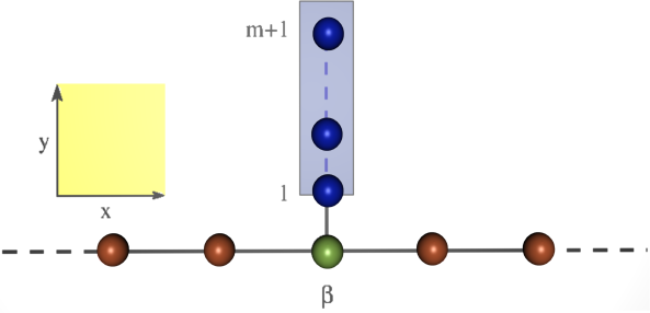
Figure 3: (Color online). Schematic representation of an $n$ times renormalized periodic lattice with an $m+1$ atom cluster attached from one side on an infinite subset of sites so that such sites get the status of $\beta$ sites (in green) in an ‘effective’ Cantor sequence.

Here, as before, $x=(E-\epsilon)/2t$, and $y=(E-\epsilon)/2\lambda$, where, $\lambda$ is the nearest neighbor hopping integral along the cluster in the $Y$-direction and has a non-zero value. Needless to say that, along the backbone that is obtained by decimating $n$ atoms, the $\alpha$ and the $\gamma$ sites (colored blue) will have the same on site potentials as given earlier, by Eq. (5), viz.,

$$\epsilon_{\alpha(\gamma)}=\epsilon+2t\frac{U_{n-1}(x)}{U_{n}(x)}$$ (7)

Let us now set $E-\epsilon_{\alpha}=E-\epsilon-2tU_{n-1}(x)/U_{n}(x)=0$, extract the (real) roots from this equation, and then set $U_{m}(y)=0$ for one such root. This immediately generates a correlation between the values of $\lambda$ and $t$.

From Eq, (6) it is evident that, the third term on the right hand side disappears with this value of the tunnel hopping $\lambda$, and hence $\epsilon_{\beta}$ becomes identical to $\epsilon_{\alpha}$ and $\epsilon_{\gamma}$. We are back with a periodically ordered array of identical on-site potentials. The stubs effectively become non-existent to an electron propagating in such a system with the above energy. The chain with the aperiodically placed stub will now transmit the electron ballistically at those special energies and no trapping will be observed.

However, we must appreciate that for each root of the equation $E-\epsilon_{\alpha}=E-\epsilon-2tU_{n-1}(x)/U_{n}(x)=0$, we shall need a different correlation between $\lambda$ and $t$. For example, for an un-renormalized backbone, that is with $n=0$, if we attach a single atom in the side coupled cluster ($m=0$), then the electron with energy $E=0$ effectively gets trapped as the lattice grows in size, as explained already. If we attach one more site in the side attachment, by making $m=1$, then the effective potential at the $\beta$ site becomes same as that of the $\alpha$ and the $\gamma$ sites and the electron traverses ballistically at $E=0$. That is, for a given relationship between $\lambda$ and $t$, just by controlling the number of QD’s in the side attachment we can make an incoming electron get trapped or transmit with undiminished amplitude of its wave function. With $m=1$, and with $n=1$, we can make the electron tunnel through the entire infinite chain ballistically at $E=0$ if we select $\lambda=\pm\sqrt{2}t$. For any other value of $\lambda$, the electron eventually gets trapped in quantum wells with increasing height and width as explained before.

Controlling trapping energy values by an external magnetic flux. – In this part, we show that, it is also possible to ‘place’ the energy eigenvalues almost anywhere in the spectrum of the ordered backbone by an external magnetic flux. For this we choose to attach quantum rings (QR) to the $\alpha$ and the $\gamma$ sites marked (artificially) on the periodic chain of atoms.

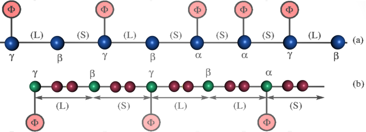
Figure 4: (Color online). (a) Periodically ordered lattice stubbed with a quantum ring to generate an artificial Cantor sequence of vertices and (b) periodic repetition of the 3rd generation Fibonacci segment $LSL$, with quantum rings side coupled to ‘create’ the Cantor geometry of $\alpha$, $\beta$ and $\gamma$ vertices.

We refer to Fig. 4. The quantum rings are are modelled with atomic sites, and are attached to the $\alpha$ and $\gamma$ sites on the periodic backbone. The $\beta$ sites are now free. This results in the effective potential at the $\alpha$ and the $\gamma$ sites, given by, $\epsilon_{\alpha}=\epsilon+\chi(E,\Phi)$, where $\chi(E,\phi)$ is the ‘correction’ added to the self energy of the bare site, obtained after renormalizing the effect of the QR. To be specific, for a $4$-site QR threaded by a uniform flux $\Phi$, the correction is given by,

$$\chi=\frac{(E-\epsilon)\left[(E-\epsilon)^{2}-2t^{2}\right]\lambda^{2}}{\left[(E-\epsilon)^{2}-2t^{2}\right]^{2}-4t^{4}\cos^{2}\frac{\pi\Phi}{\Phi_{0}}}$$ (8)

As the trapping energy values are obtained from the roots of the equation

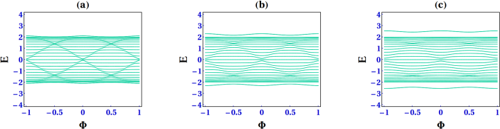
Figure 5: (Color online). Distribution of the trapping energies as the flux through a $4$-site quantum ring attached to the $\alpha$ and the $\gamma$ sites on a renormalized periodic backbone is varied. We have obtained the renormalized lattice by sequentially decimating $33$ atomic site on the initial chain. The tunnel hopping in the three panels are chosen an $\lambda=0.5$, $\lambda=1.0$ and $\lambda=2.0$ in units of the hopping integral $t$.

$E-\epsilon_{\alpha}=0$, it is obvious that, the positions of the trapping energies in the spectrum can be controlled by tuning the external flux. The energy values $E=\epsilon$ and $E=\epsilon\pm\sqrt{2}t$ are excluded of course, as at such energies $\chi=0$, and all the sites have identical on-site potentials. The propagating electron again doesn’t ‘feel’ the stubs, and the transport remains ballistic even with the aperiodic stubbing of the backbone. But for other energies, the trap is created again.

We present such an example in

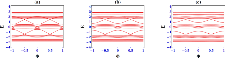
Figure 6: (Color online). Distribution of the trapping energies as the flux through a $4$-site quantum ring attached to the $\alpha$ and the $\gamma$ sites on a renormalized quasiperiodic Fibonacci backbone is varied. We have obtained the renormalized lattice by sequentially decimating the vertices on the parent chain by the deflation rule $LSL\rightarrow L$, and $LS\rightarrow S$. The tunnel hopping in the three panels are chosen an $\lambda=0.5$, $\lambda=1.0$ and $\lambda=2.0$ in units of the hopping integral $t$.

Fig. 5, where we first renormalize the periodic backbone (no stubs now) by sequentially removing $33$ sites uniformly in between two flanking sites in the chain. The renormalized periodic chain then has $\epsilon_{eff}=\epsilon+2tU(32,x)/U(33,x)$, and $t_{eff}=t/U(33,x)$, with $x=(E-\epsilon)/2t$. Then the $\alpha$, $\beta$ and $\gamma$ sites are artificially marked on this renormalized chain, following the scheme outlined before. With the $\alpha$ and the $\gamma$ sites we attach the $4$-site QR, and the ‘corrected’ self energies at these sites are obtained by adding $\chi(E,\Phi)$, as written in Eq. (8). Fig. 5 already demonstrates that the trapping energies are distributed over the entire range of the allowed spectrum of the periodic backbone, which is between $[-2,2]$ with $\epsilon$ and $t$ being chosen as zero and unity respectively. The tunnel coupling with the rings gives rise to two localized states outside the main band of energies. The localized states get shifted in energy as the tunnel hopping strength is increased from $0.5$ to $2.0$ in units of $t$.

A fractal distribution of trapping states. – It now becomes quite obvious that, the scheme of trapping an electronic excitation at specified energies is kind of universal in the sense that, it works irrespective of the structure of the ‘unit cell’ as long as we have a periodic lattice of repeating unit cells. With ‘size’ of the unit cell increasing, the trapping energies will be distributed in the manner dictated by the spectral character of the lattice when the relevant unit cell becomes, in principle, infinitely large by itself. To explain this we present in Fig. 6 the energy eigenvalues controlled by an attached array of $4$-site QR’s on special sites of a periodic lattice whose unit cell comprises an eighth generation quasiperiodic Fibonacci chain, of two ‘bonds’ $L$ and $S$.

To appreciate, we need to recall a bit that, a quasiperiodic Fibonacci chain is a prototype of a quasicrystal in one dimension, consisting of two letters, say $L$ and $S$, representing two ‘bonds’ and arranged in a sequence that grows recursively following the growth rule $L\rightarrow LS$ and $S\rightarrow L$ kohmoto . The first few generations look like $G_{1}=L$, $G_{2}=LS$, $G_{3}=LSL$, $G_{4}=LSLLS$ and so on. Any finite generation $G_{j}$ can be periodically repeated along a line to create a periodic chain with a quasiperidic geometry in its unit cell, and the spectrum of the true Fibonacci chain in its thermodynamic limit is achieved when the size of the unit cell blows up to infinity as well. The spectrum, for the sequence outlined above, is singular continuous, a Cantor set with measure zero. It typically shows a three subband structure, which exhibit self similarity on finer scan, and the wave functions are neither extended, Bloch like, nor are they exponentially localized in the Anderson sense. Instead, they are called critical.

What we do here is the following. We take, for the sake of explaining things, an eighth generation Fibonacci segment comprising $34$ bonds $L$ and $S$ set in the Fibonacci sequence, and repeat it periodically to generate our periodic chain. Then we scale the system by the standard RSRG procedure, using an extension of the usual decimation scheme, viz., $LSL\rightarrow L^{\prime}$ and $LS\rightarrow S^{\prime}$ arun . We need to identify three kinds of on site potentials for this. These are, $\epsilon_{\alpha}$, $\epsilon_{\beta}$ and $\epsilon_{\gamma}$ corresponding to the vertices flanked by $LL$, $LS$ and $SL$ bonds respectively. The hopping integrals are assigned two values, namely, $t_{L}$ and $t_{S}$ for an electron hopping across an $L$ or an $S$ bond respectively. The decimation of the lattice generates the recursion relations,

$$\epsilon_{\alpha,n} = \epsilon_{\alpha,n-1}+\frac{t_{L,n-1}^{2}\left[2E-(\epsilon_{\gamma,n-1}+\epsilon_{\beta,n-1})\right]}{(E-\epsilon_{\beta,n-1})(E-\epsilon_{\gamma,n-1})-t_{S,n-1}^{2}}$$

$$\epsilon_{\beta,n} = \epsilon_{\alpha,n-1}+\frac{t_{L,n-1}^{2}}{(E-\epsilon_{\beta,n-1})}+\frac{t_{L,n-1}^{2}(E-\epsilon_{\beta,n-1})}{(E-\epsilon_{\beta,n-1})(E-\epsilon_{\gamma,n-1})-t_{S,n-1}^{2}}$$

$$\epsilon_{\gamma,n} = \epsilon_{\gamma,n-1}+\frac{t_{S,n-1}^{2}}{E-\epsilon_{\beta,n-1}}+\frac{t_{L,n-1}^{2}(E-\epsilon_{\beta,n-1})}{(E-\epsilon_{\beta,n-1})(E-\epsilon_{\gamma,n-1})-t_{S,n-1}^{2}}$$

$$t_{L,n} = \frac{t_{L,n-1}^{2}t_{S,n-1}}{(E-\epsilon_{\beta,n-1})(E-\epsilon_{\gamma,n-1})-t_{S,n-1}^{2}}$$

$$t_{S,n} = \frac{t_{L,n-1}t_{S,n-1}}{E-\epsilon_{\beta,n-1}}$$ (9)

Using the recursion relations Eq. (9) $2n-1$ times we can ‘reduce’ a $2n+1$-th generation Fibonacci segment to a single renormalized $L$ bond, and the periodic lattice now consists of $\alpha$ sites only, with on-site potential $\epsilon_{\alpha,2n-1}$ and nearest neighbor hopping integral $t_{L,2n-1}$. On this periodic lattice, we artificially create a Cantor sequence in the spirit described before, and attach a $4$-site QR threaded by a magnetic flux at the artificial $\alpha$ and $\gamma$ site to ensure trapping at $E=\epsilon_{\alpha,2n-1}+\chi(E,\Phi)$.

In Fig. 6 we show the results, where we have reduced a $34$-bond long Fibonacci segment of $L$ and $S$ into an effective periodic lattice and then stubbed it with QR’s at appropriate sites. The initial parameters are chosen as $\epsilon_{\alpha}=\epsilon_{\beta}=\epsilon_{\gamma}=0$, a and $t_{L}=1$ and $t_{S}=2$. The diagram displays the trapping energy eigenvalues at various values of the treading magnetic flux. Interestingly, we find that, even with a nominal size of the unit cell, the three-subband structure in the energy spectrum, a typical characteristic of a Fibonacci lattice, is quite apparent. However, now one can see trapping energies located in the global gaps of the spectrum. A local Hofstadter butterfly tends to open up in the central part, around $\Phi=0$, as the strength of the tunnel hopping $\lambda$ is increased from $0.5$ to $1.0$ and then $2$, in units of $t_{L}$.

Concluding remarks –

We have shown that a perfectly periodic chain of atomic scatterers can effectively trap an electron if stubbed at an infinite deterministic set of sites. The trapping, which makes an electronic wave function form standing waves in an infinite assembly of quantum wells with a hierarchically distributed widths, can be effected at any desired scale of length. The energy values at which this takes place can be obtained using a real space renormalization group technique. The scale of length at which the trapping is observed and the locations of the stubs are intimately connected, as discussed in the paper. The energy at which one desires to trap an electron can be controlled at will by stubbing the lattice with a quantum ring threaded by a magnetic field, at a special subset of sites.The method is not restricted to the case of a non-interacting spinless electron as stated in this article, but can be applied to the propagation of waves, light waves for example, in an array of single mode waveguides. Work is in progress in this direction and the results will be published in due course.

- (1) P. W. Anderson, Phys. Rev. 109, 1492 (1958).
- (2) E. Abrahams, P. W. Anderson, D. C. Licciardello, and T. V. Ramakrishnan, Phys. Rev. Lett. 42, 673 (1979).
- (3) B. Kramer, and A. MacKinnon, Rep. Prog. Phys. 56, 1469 (1993).
- (4) C. Monthus, and T. Garel, Phys. Rev. B 81, 224208 (2010).
- (5) S. K. Lyo, Phys. Rev. Lett. 28, 1192 (1972).
- (6) S. John, Phys. Rev. Lett. 58, 2486 (1987).
- (7) E. Yablonovitch, Phys. Rev. Lett. 58, 2059 (1987).
- (8) G. Roati, C. DÉrrico, L. Fallani, M. Fattori, C. Fort, M. Zaccanti, G. Modugno, M. Modugno, and M. Inguscio, Nature (London)453, 895 (2008).
- (9) P. A. Orellana, F. Domínguez-Adame, I. Gómez, and M. L. Ladron de Guevara, Phys. Rev. B 67, 085321 (2003).
- (10) R. Farchioni, G. Grosso, and G. P. Parravicini, Phys. Rev. B 85, 165115 (2012).
- (11) A. E. Miroshnichenko, and Y. S. Kivshar, Phys. Rev. E 72, 056611 (2005).
- (12) A. E. Miroshnichenko, S. Flach, and Y. S. Kivshar, Rev. Mod. Phys. 82, 2257 (2010).
- (13) D. H. Dunlap, K. Kundu, and P. Phillips, Phys. Rev. B 40, 10999 (1989).
- (14) A. Chakrabarti, S. N. Karmakar, and R. K. Moitra, Phys. Rev. Lett. 74, 1403 (1995).
- (15) A. Chakrabarti, S. N. Karmakar, and R. K. Moitra, Phys. Rev. B 50, 13276 (1994).
- (16) A. Nandy, B. Pal, and A. Chakrabarti, Europhys. Lett. 115, 37004 (2016).
- (17) B. Pal, and A. Chakrabarti, Phys. Lett. A 378, 2782 (2014).
- (18) B. Pal, S. K. Maiti, and A. Chakrabarti, Europhys. Lett. 102, 17004 (2013).
- (19) S. Sengupta, S. Chattopadhyay, and A. Chakrabarti 344, 307 (2004).
- (20) B. Lindquist, and R. Riklund, Phys. Rev. B 56, 13902 (1997).
- (21) M. Kohmoto, B. Sutherland, and C. Tang, Phys. Rev. B 35, 1020 (1987).
- (22) A. Chakrabarti , Phys. Rev. B 74, 205313 (2006).