Unifying Theories of Time with Generalised Reactive Processes

Abstract

Hoare and He’s theory of reactive processes provides a unifying foundation for the formal semantics of concurrent and reactive languages. Though highly applicable, their theory is limited to models that can express event histories as discrete sequences. In this paper, we show how their theory can be generalised by using an abstract trace algebra. We show how the algebra, notably, allows us to also consider continuous-time traces and thereby facilitate models of hybrid systems. We then use this algebra to reconstruct the theory of reactive processes in our generic setting, and prove characteristic laws for sequential and parallel processes, all of which have been mechanically verified in the Isabelle/HOL proof assistant.

1 Introduction

The theory of reactive processes provides a generic foundation for denotational semantics of concurrent languages. It was created as part of the Unifying Theories of Programming (UTP) [1, 2] framework, which models computation using predicate calculus. The theory of reactive processes unifies formalisms such as CSP [3], ACP [4], and CCS [5]. This is made possible by its support of a large set of algebraic theorems that universally hold for families of reactive languages. The theory has been extended and applied to several languages including, stateful [6] and real-time languages, with both discrete [7] and continuous time [8, 9].

Technically, the theory’s main feature is its trace model, which provides a way for a process to record an interaction history, using an observational variable $tr:\mathop{\mathrm{seq}}\,\emph{Event}$. In the original presentation, a trace is a discrete event sequence, which is standard for languages like CSP. The alphabet can be enriched by adding further observational variables; for example, $ref:\mathop{\mathstrut{\mathbb{P}}}\nolimits\,\emph{Event}$ to model refusals [1].

Though sequence-based traces are ubiquitous for modelling concurrent systems, other models exist. In particular, the sequence-based model is insufficient to represent continuous evolution of variables as present in hybrid systems. A typical notion of history for continuous-time systems are real-valued trajectories $\mathbb{R}_{\geq 0}\to\Sigma$ over continuous state $\Sigma$.

Although the sequence and trajectory models appear substantially different, there are many similarities. For example, in both cases one can subdivide the history into disjoint parts that have been contributed by different parts of the program, and describe when a trace is a prefix of another. By characterising traces abstractly, and thus unifying these different models, we provide a generalised theory of reactive processes whose properties, operators, and laws can be transplanted into an even wider spectrum of languages. We thus enable unification of untimed, discrete-time, and continuous-time languages. The focus of our theory is on traces of finite length, but the semantic framework is extensible.

We first introduce UTP and its applications (§2). We then show how traces can be characterised algebraically by a form of cancellative monoid (§3), and that this algebra encompasses both sequences and piecewise continuous functions (§4). We apply this algebra to generalise the theory of reactive processes, and show that its key algebraic laws are retained in our generalisation, including those for sequential and parallel composition (§5).

Our work is mechanised in our theorem prover, Isabelle/UTP [10], a semantic embedding of UTP in Isabelle/HOL. We sometimes give proofs, but these merely illustrate the intuition, with the mechanisation being definitive. To the best of our knowledge, this is the most comprehensive mechanised account of reactive processes.

2 Background

UTP is founded on the idea of encoding program behaviour as relational predicates whose variables correspond to observable quantities. Unprimed variables ($x$) refer to observations at the start, and primed variables ($x^{\prime}$) to observations at a later point of the computation. The operators of a programming language are thus encoded in predicate calculus, which facilitates verification through theorem proving. For example, we can specify sequential programming operators as relations:

$$x:=v \penalty 10000\ \,\triangleq\,\,x^{\prime}=v\mathrel{\wedge}y_{1}^{\prime}=y_{1}\mathrel{\wedge}\cdots\mathrel{\wedge}y_{n}^{\prime}=y_{n}$$

$$P\mathrel{\hbox{\rm;}}Q \penalty 10000\ \,\triangleq\,\,\mathop{\mathstrut{\exists}}\nolimits x_{0}@P[x_{0}/x^{\prime}]\mathrel{\wedge}Q[x_{0}/x]$$

$$P\mathop{\hbox{\raisebox{0.0pt}{$\leftslice$}}}b\mathop{\hbox{\raisebox{0.0pt}{$\rightslice$}}}Q \penalty 10000\ \,\triangleq\,\,(b\wedge P)\vee(\neg b\wedge Q)$$

Assignment $x:=v$ states that $x^{\prime}$ takes the value $v$ and all other variables are unchanged. We define the degenerate form ${\hbox{{I \kern-10.5ptI}}}\triangleq x:=x$, which identifies all variables. Sequential composition $P\mathrel{\hbox{\rm;}}Q$ states that there exists an intermediate state $x_{0}$ on which $P$ and $Q$ agree. If-then-else conditional $P\mathop{\hbox{\raisebox{0.0pt}{$\leftslice$}}}b\mathop{\hbox{\raisebox{0.0pt}{$\rightslice$}}}Q$ states that if $b$ is true, $P$ executes, otherwise $Q$.

UTP variables can either encode program data, or behavioural information, in which case they are called observational variables. For example, we may have $ti,ti^{\prime}:\mathbb{R}_{\geq 0}$ to record the time before and after execution. These exist to enrich the semantic model and are constrained by healthiness conditions that restrict permissible behaviours. For example, we can impose $ti\leq ti^{\prime}$ to forbid reverse time travel.

Healthiness conditions are expressed as functions on predicates, such as $\hbox{{{{HT}}}}(P)\triangleq P\mathrel{\wedge}ti\leq ti^{\prime}$, the application of which coerces predicates to healthy behaviours. When such functions are idempotent and monotonic, with respect to the refinement order $\mathrel{\sqsubseteq}$, we can show, with the aid of the Knaster-Tarski theorem, that their image forms a complete lattice, which allows us to reason about recursion.

Healthiness conditions are often built from compositions: $\hbox{{{{H}}}}\triangleq\hbox{{{{H}}}}_{1}\mathrel{\circ}\hbox{{{{H}}}}_{2}\mathrel{\circ}\cdots\mathrel{\circ}\hbox{{{{H}}}}_{n}$. In this case, idempotence and monotonicity of H can be shown by proving that each $\hbox{{{{H}}}}_{i}$ is monotonic and idempotent, and each $\hbox{{{{H}}}}_{i}$ and $\hbox{{{{H}}}}_{j}$ commute. A set of healthy fixed-points, $\llbracket\hbox{{{{H}}}}\kern 1.00006pt\rrbracket\triangleq\{P|\hbox{{{{H}}}}(P)=P\}$, is called a UTP theory. Theories isolate the aspects of a programming language, such as concurrency, object orientation, and real-time programming. Theories can also be combined by composing their healthiness conditions to enable construction of sophisticated heterogeneous and integrated languages.

Our focus is the theory of reactive processes, with healthiness condition R, which we formalise in Section 5. Reactive programs, in addition to initial and final states, also have intermediate states, during which the process waits for interaction with its environment. R specifies that processes yield well-formed traces, and that, when a process is in an intermediate state, any successor must wait for it to terminate before interacting. This theory uses observational variable $wait$ to differentiate intermediate from final states, and $tr$ to record the trace.

UTP theories based on reactive processes have been applied to give formal semantics to a variety of languages [1, 11, 12], notably the Circus formal modelling language family [6], which combines stateful modelling, concurrency, and discrete time [7, 13]. A similar theory has been used for a hybrid variant of CSP [9], with a modified notion of trace. Though sharing some similarities, these various versions of reactive processes are largely disjoint theories with distinct healthiness conditions. Our contribution is to unify them all under the umbrella of generalised reactive processes.

3 Trace Algebra

In this section, we describe the trace algebra that underpins our generalised theory of reactive processes. We define traces as an abstract set $\mathcal{T}$ equipped with two operators: trace concatenation $\mathop{\,\,\widehat{}\,\,}:\mathcal{T}\to\mathcal{T}\to\mathcal{T}$, and the empty trace $\varepsilon:\mathcal{T}$, which obey the following axioms.

Definition 3.1 (Trace Algebra).

A trace algebra $(\mathcal{T},\mathop{\,\,\widehat{}\,\,},\varepsilon)$ is a cancellative monoid satisfying the following axioms:

$$x\mathop{\,\,\widehat{}\,\,}(y\mathop{\,\,\widehat{}\,\,}z) =(x\mathop{\,\,\widehat{}\,\,}y)\mathop{\,\,\widehat{}\,\,}z$$ (TA1)

$$\varepsilon\mathop{\,\,\widehat{}\,\,}x=x\mathop{\,\,\widehat{}\,\,}\varepsilon =x$$ (TA2)

$$x\mathop{\,\,\widehat{}\,\,}y=x\mathop{\,\,\widehat{}\,\,}z\,\,\mathrel{\Rightarrow}\,\,y =z$$ (TA3)

$$x\mathop{\,\,\widehat{}\,\,}z=y\mathop{\,\,\widehat{}\,\,}z\,\,\mathrel{\Rightarrow}\,\,x =y$$ (TA4)

$$x\mathop{\,\,\widehat{}\,\,}y=\varepsilon\,\,\mathrel{\Rightarrow}\,\,x =\varepsilon$$ (TA5)

As expected, $\mathop{\,\,\widehat{}\,\,}$ is associative and has left and right units. Axioms TA3 and TA4 show that $\mathop{\,\,\widehat{}\,\,}$ is injective in both arguments. As an aside, TA3 and TA4 hold only in models without infinitely long traces, as such a trace $x$ would usually annihilate $y$ in $x\mathop{\,\,\widehat{}\,\,}y$. Axiom TA5 states that there are no “negative traces”, and so if $x$ and $y$ concatenate to $\varepsilon$ then $x$ is $\varepsilon$. We can also prove the dual law: $x\mathop{\,\,\widehat{}\,\,}y=\varepsilon\,\,\mathrel{\Rightarrow}\,\,y=\varepsilon$. From this algebraic basis, we derive a prefix relation and subtraction operator.

Definition 3.2 (Trace Prefix and Subtraction).

$$x\leq y \penalty 10000\ \,\mathrel{\Leftrightarrow}\,\,\mathop{\mathstrut{\exists}}\nolimits z@y=x\mathop{\,\,\widehat{}\,\,}z$$

$$y-x \penalty 10000\ \,\triangleq\,\,\begin{cases}\iota z@y=x\mathop{\,\,\widehat{}\,\,}z&\text{if}\,x\leq y\\ \varepsilon&\text{otherwise}\end{cases}$$

Trace prefix, $x\leq y$, requires that there exists $z$ that extends $x$ to yield $y$. Trace subtraction $y-x$ obtains that trace $z$ when $x\leq y$, using the definite description operator (Russell’s $\iota$), and otherwise yields the empty trace. This is slightly different from the standard UTP operator, which is defined only when $x\leq y$. We can prove the following laws about trace prefix.

Theorem 3.1 (Trace Prefix Laws).

For $x,y,z:\mathcal{T}$,

$$(\mathcal{T},\leq)$$ is a partial order (TP1)

$$\varepsilon \leq x$$ (TP2)

$$x \leq x\mathop{\,\,\widehat{}\,\,}y$$ (TP3)

$$x\mathop{\,\,\widehat{}\,\,}y\leq x\mathop{\,\,\widehat{}\,\,}z \mathrel{\Leftrightarrow}y\leq z$$ (TP4)

TP2 tells us that $\varepsilon$ is the smallest trace, TP3 that concatenation builds larger traces, and TP4 that concatenation is monotonic in its right argument. We also have the following trace subtraction laws.

Theorem 3.2 (Trace Subtraction Laws).

$$x-\varepsilon \penalty 10000\ =\,x$$ (TS1)

$$\varepsilon-x \penalty 10000\ =\,\varepsilon$$ (TS2)

$$x-x \penalty 10000\ =\,\varepsilon$$ (TS3)

$$(x\mathop{\,\,\widehat{}\,\,}y)-x \penalty 10000\ =\,y$$ (TS4)

$$(x-y)-z \penalty 10000\ =\,x-(y\mathop{\,\,\widehat{}\,\,}z)$$ (TS5)

$$(x\mathop{\,\,\widehat{}\,\,}y)-(x\mathop{\,\,\widehat{}\,\,}z) \penalty 10000\ =\,y-z$$ (TS6)

$$y\leq x\mathrel{\wedge}x-y=\varepsilon \penalty 10000\ \mathrel{\Leftrightarrow}\,x=y$$ (TS7)

$$x\leq y \penalty 10000\ \mathrel{\Rightarrow}\,x\mathop{\,\,\widehat{}\,\,}(y-x)=y$$ (TS8)

Laws TS1-TS3 relate trace subtraction and the empty trace. TS4 shows that subtraction inverts concatenation. TS5 shows that subtracting two traces is equivalent to subtracting their concatenation. TS6 shows that subtraction can be used to remove a common prefix. TS7 shows that two traces are equal if, and only if, the first is a prefix of the second and they subtract to $\varepsilon$. TS8 shows that a trace can be split into its prefix and suffix.

In the next section, we show that standard notions of traces are models. Afterwards, in Section 5 we use the algebra to create the generalised theory of reactive processes.

4 Trace Models

In this section we describe three trace models: positive reals, finite sequences, and timed traces. Other models are possible; for example, we can further extend timed traces to “super-dense time” [14] to encompass multiple distinguished discrete state updates at a time instant. We leave study of other models as future work.

Positive real numbers $\mathbb{R}_{\geq 0}$ form one of the simplest models of the trace algebra.

Theorem 4.1.

$(\mathbb{R}_{\geq 0},+,0)$ is a trace algebra.

Proof.

$+$ is clearly associative, cancellative, and has $0$ as its left and right unit. Moreover, since $+$ is commutative and $\mathbb{R}_{\geq 0}$ contains no negative numbers then $+$ has no additive inverse. ∎

Positive reals can be used to express timed programs with a clock variable $time:\mathbb{R}_{\geq 0}$ [15]. Finite sequences, unsurprisingly, also form a trace algebra, when we set $\mathop{\,\,\widehat{}\,\,}$ to sequence concatenation ($\mathbin{\smash{\raise 3.44444pt\hbox{$\smallfrown$}}}$), and $\varepsilon$ to the empty sequence ($\langle\rangle$).

Theorem 4.2.

$(\mathop{\mathrm{seq}}\,\textit{Event},\mathbin{\smash{\raise 3.44444pt\hbox{$\smallfrown$}}},\langle\rangle)$ is a trace algebra.

Though simple, we note that the sequence-based trace model has been shown to be sufficient to characterise both untimed [6] and discrete time modelling languages [13].

A more complex model is that of piecewise continuous functions, for which we adopt and refine a model called timed traces ($\mathbb{T}\!\mathbb{T}$) [16]. A timed trace is a partial function of type $\mathbb{R}_{\geq 0}\mathrel{\ooalign{\hfil$\mapstochar\mkern 5.0mu$\hfil\cr$\rightarrow$}}\Sigma$, for continuous state type $\Sigma$, which represents the system’s continuous evolution with respect to time.

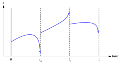
Figure 1: Piecewise continuous timed traces

In our model we also require that timed traces be piecewise continuous, to allow both continuous and discrete information. A timed trace is split into a finite sequence of continuous segments, as shown in Figure 1. Each segment accounts for a particular evolution of the state interspersed with discontinuous discrete events. This necessitates that we can describe limits and continuity, and consequently we require that $\Sigma$ be a topological space, such as $\mathbb{R}^{n}$, though it can also contain discrete topological information, like events. Continuous variables are projections such as $x:\Sigma\to\mathbb{R}$. We give the formal model below.

Definition 4.1 (Timed Traces).

$$\begin{array}[]{ll}\mathbb{T}\!\mathbb{T}\triangleq&\!\!\left\{\begin{array}[]{ll}f:\mathbb{R}_{\geq 0}\mathrel{\ooalign{\hfil$\mapstochar\mkern 5.0mu$\hfil\cr$\rightarrow$}}\Sigma\\ |\,\mathop{\mathstrut{\exists}}\nolimits t:\mathbb{R}_{\geq 0}@\mathop{\mathrm{dom}}(f)=[0,t)\\ \qquad\mathrel{\wedge}t>0\mathrel{\Rightarrow}\mathop{\mathstrut{\exists}}\nolimits I:\mathbb{R}_{\textnormal{oseq}}\\ \,\,@\left(\begin{array}[]{l}\mathop{\mathrm{ran}}(I)\subseteq[0,t]\\ \mathrel{\wedge}\{0,t\}\subseteq\mathop{\mathrm{ran}}(I)\\ \mathrel{\wedge}\left(\begin{array}[]{l}\mathop{\mathstrut{\forall}}\nolimits n<\#I-1@\\ \,f\mathop{\,\textsf{cont-on}\,}[I_{n},I_{n+1})\end{array}\!\right)\end{array}\!\right)\end{array}\right\}\end{array}$$

$\begin{array}[]{l}\mathbb{R}_{\mathsf{oseq}}\triangleq\{x:\textnormal{seq}\,\mathbb{R}\,|\,\mathop{\mathstrut{\forall}}\nolimits n<\#{x}-1@x_{n}<x_{n+1}\}\\[4.30554pt] f\mathop{\,\textsf{cont-on}\,}[m,n)\triangleq\mathop{\mathstrut{\forall}}\nolimits t\in[m,n)@\underset{x\to t^{+}}{\lim}\,f(x)=f(t)\end{array}$

A timed trace is a partial function $f$ with domain $[0,t)$, for end point $t\geq 0$. When the trace is non-empty $(t>0)$, there exists an ordered sequence of instants $I$ giving the bounds of each segment. $\mathbb{R}_{\mathsf{oseq}}$ is the subset of finite real sequences such that for every index $n$ in the sequence less than its length $\#{x}$, $x_{n}<x_{n+1}$. $I$ must naturally contain at least $0$ and $t$, and only values between these two extremes. The timed trace $f$ is required to be continuous on each interval $[I_{n},I_{n+1})$. The operator $f\mathop{\,\textsf{cont-on}\,}A$ denotes that $f$ is continuous on the range given by $A$. We now introduce the core timed trace operators, which take inspiration from Höfner’s algebraic trajectories [17].

Definition 4.2 (Timed-trace Operators).

$$\begin{array}[]{rcl}\textnormal{end}(f)&\,\,\triangleq&\mathrm{min}(\mathbb{R}_{\geq 0}\setminus\mathop{\mathrm{dom}}(f))\\[4.30554pt] \varepsilon&\,\,\triangleq&\emptyset\\[4.30554pt] f\mathop{\,\,\widehat{}\,\,}g&\,\,\triangleq&f\cup(g\bm{\gg}\textnormal{end}(f))\end{array}$$

Auxiliary function $f\bm{\gg}n$ shifts the indices of a partial function $f:\mathbb{R}_{\geq 0}\mathrel{\ooalign{\hfil$\mapstochar\mkern 5.0mu$\hfil\cr$\rightarrow$}}A$ to the right by $n:\mathbb{R}_{\geq 0}$, and has definition $\mathop{\mathstrut{\lambda}}\nolimits x@f(x-n)$. The operator $\textnormal{end}(f)$ gives the end time of a trace $f:\mathbb{T}\!\mathbb{T}$ by taking the infimum of the real numbers excluding the domain of $f$. The empty trace $\varepsilon$ is the empty function. Finally, $f\mathop{\,\,\widehat{}\,\,}g$ shifts the domain of $g$ to start at the end of $f$, and takes the union. We establish laws governing these trace operators.

Theorem 4.3 (Timed-trace Laws).

$$(f\bm{\gg}m)\bm{\gg}n =f\bm{\gg}(m+n)$$ (T1)

$$(f\cup g)\bm{\gg}n =(f\bm{\gg}n)\cup(g\bm{\gg}n)$$ (T2)

$$\textnormal{end}(\varepsilon) =0$$ (T3)

$$\textnormal{end}(x\mathop{\,\,\widehat{}\,\,}y) =\textnormal{end}(x)+\textnormal{end}(y)$$ (T4)

T1 shows that shifting a function twice equates to a single shift on their summation. T2 shows that shift distributes through function union. T3 shows that the length of the empty trace is $0$, and T4 shows that the length of a trace is the sum of its parts. $\mathbb{T}\!\mathbb{T}$ is closed under trace concatenation.

Theorem 4.4 (Trace Concatenation Closure).

If there exists $m,n:\mathbb{R}_{\geq 0}$, such that $\mathop{\mathrm{dom}}(tt_{1})=[0,m)$, and $\mathop{\mathrm{dom}}(tt_{2})=[0,n)$, then $tt_{1},tt_{2}\in\mathbb{T}\!\mathbb{T}$ if, and only if, $tt_{1}\mathop{\,\,\widehat{}\,\,}tt_{2}\in\mathbb{T}\!\mathbb{T}$.

This theorem tells us that decomposition of a timed trace always yields timed traces, provided both $f$ and $g$ have a contiguous domain. Finally, trace concatenation satisfies our trace algebra.

Theorem 4.5.

$(\mathbb{T}\!\mathbb{T},\mathop{\,\,\widehat{}\,\,},\varepsilon)$ forms a trace algebra

Proof.

For illustration, we show the derivation for associativity. The other proofs are simpler.

$$x \mathop{\,\,\widehat{}\,\,}(y\mathop{\,\,\widehat{}\,\,}z)$$

$$=x\cup((y\cup(z\bm{\gg}\textnormal{end}(y))\bm{\gg}\textnormal{end}(x))$$

$$=x\cup((y\bm{\gg}\textnormal{end}(x))\cup(z\bm{\gg}\textnormal{end}(y)\bm{\gg}\textnormal{end}(x)))$$

$$=(x\cup(y\bm{\gg}\textnormal{end}(x)))\cup(z\bm{\gg}(\textnormal{end}(x)+\textnormal{end}(y)))$$

$$=(x\mathop{\,\,\widehat{}\,\,}y)\cup(z\bm{\gg}(\textnormal{end}(x)+\textnormal{end}(y)))$$

$$=(x\mathop{\,\,\widehat{}\,\,}y)\cup(z\bm{\gg}(\textnormal{end}(x\mathop{\,\,\widehat{}\,\,}y)))$$

$$=(x\mathop{\,\,\widehat{}\,\,}y)\mathop{\,\,\widehat{}\,\,}z$$

∎

This model provides the basis for hybrid computation. We introduce the theory in the next section.

5 Generalised Reactive Processes

Here, we use our trace algebra to provide a generalised theory of reactive processes. We prove the key laws of reactive processes, thus demonstrating the conservative nature of our theory. Many of the properties here have been previously proved [2], but we restate and prove many of them due to our weakening of the trace model and some small differences. Another novelty is that all these theorems have been mechanised in our Isabelle/UTP repository. Following [1, 2] we define the theory in terms of two pairs of observational variables:

• $wait,wait^{\prime}:\mathbb{B}$ – describe when the previous or current process, respectively, is in an intermediate state;

• $tr,tr^{\prime}:\mathcal{T}$ – the trace that occurred prior to and after execution of the current process in terms of a trace algebra $(\mathcal{T},\mathop{\,\,\widehat{}\,\,},\varepsilon)$.

Our theory does not contain refusal variables $ref,ref^{\prime}$, as these are not always necessary to describe reactive processes [13]. We describe three healthiness conditions namely R1, $\hbox{{{{R2}}}}_{c}$, and R3. R1 and R3 are already presented in [1]; for their R2 we have a different formulation, which we call $\hbox{{{{R2}}}}_{c}$.

Definition 5.1 (Reactive Healthiness Conditions).

$$\hbox{{{{R1}}}}(P) \penalty 10000\ \triangleq\,P\mathrel{\wedge}tr\leq tr^{\prime}$$

$$\hbox{{{{R2}}}}_{c}(P) \penalty 10000\ \triangleq\,P[\varepsilon,tr^{\prime}-tr/tr,tr^{\prime}]\mathop{\hbox{\raisebox{0.0pt}{$\leftslice$}}}tr\leq tr^{\prime}\mathop{\hbox{\raisebox{0.0pt}{$\rightslice$}}}P$$

$$\hbox{{{{R3}}}}(P) \penalty 10000\ \triangleq\,{\hbox{{I \kern-10.5ptI}}}\mathop{\hbox{\raisebox{0.0pt}{$\leftslice$}}}wait\mathop{\hbox{\raisebox{0.0pt}{$\rightslice$}}}P$$

R $$\penalty 10000\ \triangleq\,\hbox{{{{R3}}}}\mathrel{\circ}\hbox{{{{R2}}}}_{c}\mathrel{\circ}\hbox{{{{R1}}}}$$

R1 states that $tr$ is monotonically increasing; processes are not permitted to undo past events. $\hbox{{{{R2}}}}_{c}$ states that a process must be history independent: the only part of the trace it may constrain is $tr^{\prime}-tr$, that is, the portion since the previous observation $tr$. Specifically, if the history is deleted, by substituting $\varepsilon$ for $tr$ and $tr^{\prime}-tr$ for $tr^{\prime}$, then the behaviour of the process is unchanged. Our formulation of $\hbox{{{{R2}}}}_{c}$ deletes the history only when $tr\leq tr^{\prime}$, which ensures that $\hbox{{{{R2}}}}_{c}$ does not depend on R1, and thus commutes with it. Finally, R3 states that if a prior process is intermediate ($wait^{\prime}$) then the current process must identify all variables.

We compose the three to yield R, the overall healthiness condition of reactive processes. An example R healthy predicate is

$$\hbox{{{{R3}}}}(tr^{\prime}=tr\mathop{\,\,\widehat{}\,\,}\langle a\rangle\mathrel{\wedge}v^{\prime}=v)$$

which extends the trace with a single event $a$ and leaves program variable $v$ unchanged. We show that R is idempotent and monotonic.

Theorem 5.1 (R idempotence and monotonicity).

$$\hbox{{{{R}}}}=\hbox{{{{R}}}}\mathrel{\circ}\hbox{{{{R}}}}\text{\penalty 10000\ \penalty 10000\ and\penalty 10000\ \penalty 10000\ }P\mathrel{\sqsubseteq}Q\mathrel{\Rightarrow}\hbox{{{{R}}}}(P)\mathrel{\sqsubseteq}\hbox{{{{R}}}}(Q)$$

A corollary of Theorem 5.1 is that reactive processes form a complete lattice.

Theorem 5.2.

Reactive processes form a complete lattice ordered by $\mathrel{\sqsubseteq}$, with infimum $\bigsqcap{}_{\!\textit{{\tiny R}}}\,\,A$ and supremum $\bigsqcup{}_{\!\textit{{\tiny R}}}\,\,A$, for $A\subseteq\llbracket\hbox{{{{R}}}}\kern 1.00006pt\rrbracket$.

This, in particular, provides us with specification and reasoning facilities about recursive reactive processes using the fixed-point operators.

Having stated the lattice theoretic properties of reactive processes, we move onto the relational operators. Intuitively, R1 and $\hbox{{{{R2}}}}_{c}$ together ensure that the reactive behaviour of a process contributes an extension $t$ to the trace.

Theorem 5.3 (R1-$\hbox{{{{R2}}}}_{c}$ trace contribution).

$$\hbox{{{{R1}}}}(\hbox{{{{R2}}}}_{c}(P))=(\mathop{\mathstrut{\exists}}\nolimits t@P[\varepsilon,t/tr,tr^{\prime}]\mathrel{\wedge}tr^{\prime}=tr\mathop{\,\,\widehat{}\,\,}t)$$

This shows that for any R1-$\hbox{{{{R2}}}}_{c}$ process there exists a trace extension $t$ recording its behaviour, and that $tr^{\prime}$ is the prior history appended with this extension. Aside from illustrating R1 and $\hbox{{{{R2}}}}_{c}$, this allows us to restate a process containing $tr$ and $tr^{\prime}$ to one with only the extension logical variable $t$, which provides a more natural entry point for reasoning about the trace contribution of a process. In particular, we can prove a related law about sequential composition of reactive processes.

Theorem 5.4 (R1-$\hbox{{{{R2}}}}_{c}$ sequential).

If $P$ and $Q$ are R1-$\hbox{{{{R2}}}}_{c}$ healthy, then

$$P\mathrel{\hbox{\rm;}}Q=\mathop{\mathstrut{\exists}}\nolimits t_{1},t_{2}@(( P[\varepsilon,t_{1}/tr,tr^{\prime}]\mathrel{\hbox{\rm;}}$$

$$Q[\varepsilon,t_{2}/tr,tr^{\prime}])\mathrel{\wedge}$$

$$tr^{\prime}=tr\mathop{\,\,\widehat{}\,\,}t_{1}\mathop{\,\,\widehat{}\,\,}t_{2})$$

Proof.

By Theorem 5.3 and relational calculus. ∎

This theorem shows that two sequentially composed processes have their own unique contribution to the trace without sharing or interference. When applied in the context of a timed trace, for example, it allows us to subdivide the trajectory into segments, which we can reason about separately. This theorem allows us to demonstrate closure of R1-$\hbox{{{{R2}}}}_{c}$ predicates under sequential composition.

Theorem 5.5 (R1-$\hbox{{{{R2}}}}_{c}$ sequential closure).

If $P$ and $Q$ are both R1 and $\hbox{{{{R2}}}}_{c}$ healthy then

$$\hbox{{{{R1}}}}(\hbox{{{{R2}}}}_{c}(P\mathrel{\hbox{\rm;}}Q))=P\mathrel{\hbox{\rm;}}Q$$

Closure of R3 has previously been shown [2] and we have mechanised this proof. This allows us to prove the following theorem.

Theorem 5.6 (R sequential closure).

If $P$ and $Q$ are both R healthy then $P\mathrel{\hbox{\rm;}}Q$ is R healthy.

We have now shown that reactive processes are closed under the lattice and relational operators, and can use these results to demonstrate the algebraic nature of the theory, by showing that reactive processes form a weak unital quantale.

Theorem 5.7.

R predicates form a weak unital quantale. Provided $A\subseteq\llbracket\hbox{{{{R}}}}\kern 1.00006pt\rrbracket$ and $A\neq\emptyset$ the following laws hold:

$$P\mathrel{\hbox{\rm;}}(\bigsqcap{}_{\!\textit{{\tiny R}}}\,\,A) =(\bigsqcap{}_{\!\textit{{\tiny R}}}\,Q\in A@P\mathrel{\hbox{\rm;}}Q)$$ (Q1)

$$(\bigsqcap{}_{\!\textit{{\tiny R}}}\,\,A)\mathrel{\hbox{\rm;}}Q =(\bigsqcap{}_{\!\textit{{\tiny R}}}\,P\in A@P\mathrel{\hbox{\rm;}}Q)$$ (Q2)

$$P\mathrel{\hbox{\rm;}}{\hbox{{I \kern-10.5ptI}}} ={\hbox{{I \kern-10.5ptI}}}\mathrel{\hbox{\rm;}}P=P$$ (Q3)

Proof.

Since $\bigsqcap{}_{\!\textit{{\tiny R}}}\,\,A=\hbox{{{{R}}}}(\bigsqcap A)$ and sequential composition left and right distributes through $\bigsqcap$ it suffices, to show that R is continuous: it distributes through non-empty infima. ∎

Q1 and Q2 are the quantale laws, which state that sequential composition distributes through infima. The requirement of non-emptiness is why the quantale is called “weak”. Finally, Q3 makes the weak quantale unital. Unital quantales are an important algebraic structure that give rise to Kleene algebras [18]. They augment a complete lattice with the laws above, the combination of which provides a minimal algebraic foundation for substantiating the point-free laws of sequential programming [18].

Our final result is closure under parallel composition. The UTP provides an operator called parallel-by-merge [1], $P\mathrel{\parallel}_{M}Q$, whereby the composition of processes $P$ and $Q$ separates their states, calculates their independent concurrent behaviours, and then merges the results. The operator is parametric over merge predicate $M$ that specifies how synchronisation is performed. Different programming language semantics require formation of a bespoke merge predicate depending on their concurrency scheme. We give a slightly simplified version of the UTP definition, which is nevertheless equivalent.

Definition 5.2 (Parallel-by-merge).

$$P\mathrel{\parallel}_{M}Q\,\triangleq\,(\lceil P\rceil_{0}\mathrel{\wedge}\lceil Q\rceil_{1}\mathrel{\wedge}v^{\prime}=v)\mathrel{\hbox{\rm;}}M$$

Operator $\lceil P\rceil_{n}$ augments the after variables of $P$ with an index; for example:

$$\lceil x^{\prime}=7\cdot y\rceil_{0}=(0.x^{\prime}=7\cdot y)$$

The three conjuncts rename the after variables of $P$ and $Q$ to ensure no clashes, and copy all before variables ($v$) to after variables, respectively. Thus, $M$ has access to the state of each variable before execution ($v$), and from the respective composed processes ($0.v$ and $1.v$). Merge predicate $M$ can then invoke $tr^{\prime}=f(0.tr,1.tr)$ with a suitable trace merge function $f$, such as interleaving.

The healthiness conditions R1 and R3 can be directly applied to $M$, modulo some differences in alphabet. $\hbox{{{{R2}}}}_{c}$ requires adaptation as it is possible to access the trace history through the two indexed traces, $0.tr$ and $1.tr$, in addition to $tr$. It is, therefore, necessary to delete the history from the two in the revised healthiness condition $\hbox{{{{R2}}}}_{m}$ below.

Definition 5.3 ($\hbox{{{{R2}}}}_{c}$ for merge predicates).

$$\hbox{{{{R2}}}}_{m}(M) \triangleq(P[\varepsilon,tr^{\prime}\!-\!tr,0.tr\!-\!tr,1.tr\!-\!tr$$

$$\qquad\,\,/tr,tr^{\prime},0.tr,1.tr])\mathop{\hbox{\raisebox{0.0pt}{$\leftslice$}}}tr\leq tr^{\prime}\mathop{\hbox{\raisebox{0.0pt}{$\rightslice$}}}P$$

$\hbox{{{{R2}}}}_{m}$ has the same form as $\hbox{{{{R2}}}}_{c}$ except that it deletes the history of three extant traces, $tr^{\prime}$, $0.tr$, and $1.tr$. From $M$’s perspective, $0.tr$ and $1.tr$ contain the trace the parallel processes have executed. Thus we need to delete the history, through substitution, from these as well so that they contain only the contributions of their respective processes. This allows us to show that the overall composition is $\hbox{{{{R2}}}}_{c}$. We define a condition for merge predicates – $\hbox{{{{R}}}}_{m}\triangleq\hbox{{{{R1}}}}\mathrel{\circ}\hbox{{{{R2}}}}_{m}\mathrel{\circ}\hbox{{{{R3}}}}$ – and prove the following final theorem.

Theorem 5.8.

$P\mathrel{\parallel}_{M}Q$ is R healthy provided that $P,Q$ are R healthy, and $M$ is $\hbox{{{{R}}}}_{m}$ healthy.

Thus our generalised theory of reactive processes is conservative and unifies the denotational semantics of concurrent programming.

6 Conclusion

Traces are ubiquitous in modelling of program history. Here, we have shown how a generalised foundation for their semantics can be given in terms of a trace algebra, and presented some important models, notably piecewise-continuous functions. Finally, we have applied it to reconstruct Hoare and He’s model of reactive processes, with some important additions of our own, including revision of R2, additional theorems about reactive relations, and lifting of the healthiness conditions to parallel composition. All of the theorems described herein have been mechanised in Isabelle/UTP [10].

In the future we will apply this theory of reactive processes to give a new model to the UTP hybrid relational calculus [8] that we have previously created to give denotational semantics to Modelica and Simulink. Moreover, inspired by [6], we will use our theory to describe generalised reactive designs, a UTP theory that justifies combined use of concurrent and assertional reasoning. This will enable the construction of verification tools on top of our Isabelle/HOL embedding for concurrent and hybrid programming languages.

We also aim to explore weakenings of the trace algebra and healthiness conditions to support larger classes of reactive process semantics. For example, weakening of the trace cancellation laws could enable representation of infinite traces in order to support reactive processes with unbounded nondeterminism. Moreover, $\hbox{{{{R2}}}}_{c}$ currently prevents a process from depending on an absolute start time with respect to a global clock. In the future this could be relaxed, either at the model or theory level, to support time variant real-time and hybrid processes.

References

- [1] C. A. R. Hoare, J. He, Unifying Theories of Programming, Prentice-Hall, 1998.
- [2] A. Cavalcanti, J. Woodcock, A tutorial introduction to CSP in Unifying Theories of Programming, in: Refinement Techniques in Software Engineering, Vol. 3167 of LNCS, Springer, 2006, pp. 220–268.
- [3] C. A. R. Hoare, Communicating Sequential Processes, Prentice-Hall, 1985.
- [4] J. A. Bergstra, J. W. Klop, Process algebra for synchronous communication, Information and Control 60 (1–3) (1984) 109–137.
- [5] R. Milner, Communication and Concurrency, Prentice Hall, 1989.
- [6] M. Oliveira, A. Cavalcanti, J. Woodcock, A UTP semantics for Circus, Formal Aspects of Computing 21 (2009) 3–32.
- [7] K. Wei, J. Woodcock, A. Cavalcanti, Circus Time with Reactive Designs, in: Unifying Theories of Programming, Vol. 7681 of LNCS, Springer, 2013, pp. 68–87.
- [8] S. Foster, B. Thiele, A. Cavalcanti, J. Woodcock, Towards a UTP semantics for Modelica, in: Proc. 6th Intl. Symp. on Unifying Theories of Programming, Vol. 10134 of LNCS, Springer, 2016, pp. 44–64.
- [9] J. He, From CSP to hybrid systems, in: A. W. Roscoe (Ed.), A classical mind: essays in honour of C. A. R. Hoare, Prentice Hall, 1994, pp. 171–189.
- [10] S. Foster, F. Zeyda, J. Woodcock, Unifying heterogeneous state-spaces with lenses, in: Proc. 13th Intl. Conf. on Theoretical Aspects of Computing (ICTAC), Vol. 9965 of LNCS, Springer, 2016, pp. 295–314.
- [11] M. Smith, A unifying theory of true concurrency based on CSP and lazy observation, in: Communicating Process Architectures, IOS Press, 2005, pp. 177–188.
- [12] L. Zhu, Q. Xu, J. He, H. Zhu, A formal model for a hybrid programming language, in: D. Naumann (Ed.), UTP, Vol. 8963 of LNCS, Springer, 2014, pp. 125–142.
- [13] J. Woodcock, Engineering UToPiA - Formal Semantics for CML, in: FM 2014: Formal Methods, Vol. 8442 of LNCS, Springer, 2014, pp. 22–41.
- [14] E. A. Lee, Constructive models of discrete and continuous physical phenomena, IEEE Access 2 (2014) 797–821.
- [15] I. J. Hayes, S. E. Dunne, L. Meinicke, Unifying theories of programming that distinguish nontermination and abort, in: Mathematics of Program Construction (MPC), Vol. 6120 of LNCS, Springer, 2010, pp. 178–194.
- [16] I. Hayes, Termination of real-time programs: Definitely, definitely not, or maybe, in: S. Dunne, B. Stoddart (Eds.), Proc. 1st Intl. Symp. on Unifying Theories of Programming, Vol. 4010 of LNCS, Springer, 2006, pp. 141–154.
- [17] P. Höfner, B. Möller, An algebra of hybrid systems, Journal of Logic and Algebraic Programming 78 (2) (2009) 74–97.
- [18] A. Armstrong, V. Gomes, G. Struth, Building program construction and verification tools from algebraic principles, Formal Aspects of Computing 28 (2) (2015) 265–293.