Toda conformal blocks, quantum groups, and flat connections

Abstract

This paper investigates the relations between the Toda conformal field theories, quantum group theory and the quantisation of moduli spaces of flat connections. We use the free field representation of the ${\mathcal{W}}$-algebras to define natural bases for spaces of conformal blocks of the Toda conformal field theory associated to the Lie algebra ${\mathfrak{s}}{\mathfrak{l}}_{3}$ on the three-punctured sphere with representations of generic type associated to the three punctures. The operator-valued monodromies of degenerate fields can be used to describe the quantisation of the moduli spaces of flat $\mathrm{SL}(3)$-connections. It is shown that the matrix elements of the monodromies can be expressed as Laurent polynomials of more elementary operators which have a simple definition in the free field representation. These operators are identified as quantised counterparts of natural higher rank analogs of the Fenchel-Nielsen coordinates from Teichmüller theory. Possible applications to the study of the non-Lagrangian SUSY field theories are briefly outlined.

1 Introduction

Relations between conformal field theories (CFTs), quantum groups and the quantisation of moduli spaces of flat connections have been investigated extensively in the past in connection with the Chern-Simons theory with compact gauge groups. It can be expected that this subject has a somewhat richer counterpart in the cases where the gauge group becomes non-compact. Interest in the non-compact cases is motivated in particular by recent development in supersymmetric field theory, as will be briefly outlined next.

1.1 Motivation from ${\mathcal{N}}=2$ supersymmetric field theory

An important source of motivation for the study of the non-compact cases are the relations between ${\mathcal{N}}=2$ supersymmetric field theories in four dimensions and two-dimensional conformal field theories discovered in [AGT]. This development is deeply related to the study of the relations between $d=4$, ${\mathcal{N}}=2$ supersymmetric field theories and quantum integrable models initiated in [NS]. An interesting class $d=4$, ${\mathcal{N}}=2$ supersymmetric field theories, nowadays often referred to as class ${\mathcal{S}}$, consists of theories $\mathfrak{X}(C,\mathfrak{g})$ labelled by a Riemann surface $C$ and a Lie algebra $\mathfrak{g}$ of ADE-type [Ga, GMN]. The theory $\mathfrak{X}(C,\mathfrak{g})$ on a four-manifold $M^{4}$ is believed to be the effective description for the six-dimensional $(2,0)$ theory associated to ${\mathfrak{g}}$ on $M^{4}\times C$ when the area of $C$ is small. In the simplest case where $\mathfrak{g}=\mathfrak{sl}_{2}$ an essential role in this story is played by the algebra ${\mathcal{A}}_{\mathfrak{X}}$ of supersymmetric Wilson and ’t Hooft loops representing an important sub-algebra of the algebra of all observables in $\mathfrak{X}(C,\mathfrak{g})$. The algebra ${\mathcal{A}}_{\mathfrak{X}}$ turns out to be isomorphic to the algebra ${\mathcal{A}}_{V}$ of Verlinde line operators in Liouville CFT [AGGTV, DGOT, GOP, IOT], which is furthermore isomorphic to the algebra ${\mathcal{A}}_{\mathcal{M}}$ of quantised functions on the moduli space of flat $\mathrm{SL}(2)$-connections on Riemann surfaces [TV], as summarised in Table 1.

Field theory $\mathfrak{X}(C,\mathfrak{sl}_{2})$	Liouville theory	Moduli of flat connections on $C$
Algebra ${\mathcal{A}}_{\mathfrak{X}}$ generated by	Algebra ${\mathcal{A}}_{V}$ of Verlinde	Quantised algebra ${\mathcal{A}}_{\mathcal{M}}$ of
SUSY loop observables	line operators	functions on ${\mathcal{M}}_{\rm flat}(\mathrm{SL}(2),C)$
Instanton partition	Liouville conformal	Natural bases for
functions	blocks	modules of ${\mathcal{A}}_{\mathcal{M}}$

Table 1: Isomorphic algebras appear in different contexts.

One can argue [TV] that the isomorphisms between the algebras ${\mathcal{A}}_{\mathfrak{X}}$, ${\mathcal{A}}_{V}$ and ${\mathcal{A}}_{M}$ imply the relations between instanton partition functions for $\mathfrak{X}(C,\mathfrak{sl}_{2})$ and conformal blocks of Liouville CFT observed in [AGT] and discussed in many subsequent works.

In the cases where ${\mathfrak{g}}$ is a Lie algebra of higher rank one still expects to find a similar picture with Liouville CFT replaced by the conformal Toda CFTs associated to finite-dimensional Lie algebras ${\mathfrak{g}}$. However, even in the next simplest case $\mathfrak{g}=\mathfrak{sl}_{3}$ one encounters considerable additional difficulties obstructing direct generalisations of the results known for $\mathfrak{g}=\mathfrak{sl}_{2}$. On the side of ${\mathcal{N}}=2$ SUSY field theory one generically finds interacting field theories not having a weak coupling limit with a useful Lagrangian description. It is not known how to calculate the partition functions in these cases. This difficulty has a counterpart on the side of Toda CFT where the spaces of conformal blocks are known to be infinite dimensional generically, but otherwise poorly understood up to now.

This paper is a step towards the generalisation of the correspondences between the theories $\mathfrak{X}(C,\mathfrak{g})$ and Toda CFT to the cases where no Lagrangian description is known. Motivated by the six-dimensional description of $\mathfrak{X}(C,\mathfrak{g})$, we take the quantised algebra of functions ${\mathcal{A}}_{\mathcal{M}}$ as an ansatz for the algebra ${\mathcal{A}}_{\mathfrak{X}}$. This is perfectly consistent with previous work on the cases which do have a Lagrangian description [Bu, GLF1, GLF2, LF]. The relations between representations of ${\mathcal{A}}_{\mathcal{M}}$ and the algebra of Verlinde line operators in Toda CFT investigated in [CGT] suggest that suitable Toda conformal blocks represent natural candidates for the as yet unknown partition functions of the strongly coupled theories $\mathfrak{X}(C,\mathfrak{g})$. This paper provides groundwork for such a program in the simplest nontrivial case ${\mathfrak{g}}=\mathfrak{sl}_{3}$.

Our work is furthermore motivated by the papers [BMPTY, MP, IMP] where it was proposed that the conformal blocks of Toda CFT can be obtained in a certain limit from the partition functions of topological string theory on certain toric Calabi-Yau manifolds used for the geometric engineering of $\mathfrak{X}(C,\mathfrak{g})$. With the help of the refined topological vertex one may represent the relevant topological string partition functions as infinite series admitting partial resummations. If the geometric engineering limit of these partition functions can be taken, it is expected to represent conformal blocks in Toda CFT. However, at the moment it is not known if this is the case and which basis for the conformal blocks in Toda CFT the topological string partition functions will correspond to. Only when this question is answered one can extract predictions for the Toda three point functions from the results of [BMPTY, MP, IMP]. We’ll address the connections to topological string theory in subsequent papers.

1.2 Context

One of our goals is to establish a precise relation between conformal blocks in Toda CFT and specific states in the space of states obtained by quantising the moduli spaces of flat connections on Riemann surfaces $C$. The use of pants decompositions reduces the problem to the basic case $C=C_{0,3}$. Some guidance is provided by the paradigm well-studied in the case of rational conformal field theories summarised in Table 2.

Conformal field theory	Quantum group theory	Moduli of flat connections
Invariants in tensor products	Invariants in tensor products of	States
of ${\mathcal{W}}$-algebra representations	quantum group representations
(conformal blocks)

Table 2: Comparison of modular functors from conformal field theory, quantum group theory (Reshetikhin-Turaev construction) and quantisation of the moduli spaces of flat connections on Riemann surfaces.

However, the Toda CFTs of interest in this context are not expected to be rational CFTs. We’ll therefore need a non-rational analog of the set of relations indicated in Table 2 generalising the situation encountered in the case of Liouville theory, see [TV] and references therein. The experiences made in this case suggest that a very useful role will be played in the non-rational cases by the Verlinde line operators, a natural family of operators ${\mathsf{V}}_{\gamma}$ on the spaces of conformal blocks labelled by closed curves $\gamma$ on the Riemann surface $C$. The relevant spaces of conformal blocks can be abstractly characterised as modules for the algebra ${\mathcal{A}}_{V}$ of Verlinde line operators [TV]. This means that these spaces of conformal blocks have a natural scalar product making the Verlinde line operators self-adjoint. Natural representations of ${\mathcal{A}}_{V}$ diagonalise maximal commutative sub-algebras of ${\mathcal{A}}_{V}$. Such sub-algebras of ${\mathcal{A}}_{V}$ are labelled by pants decompositions. Different pants decompositions give different representations of ${\mathcal{A}}_{V}$ intertwined by unitary operators representing the fusion, braiding and modular transformations.

A key step towards understanding the relation between conformal field theory and the quantum theory of flat connections is therefore to establish the isomorphism between the algebra of Verlinde line operators ${\mathcal{A}}_{V}$ and the algebra of quantised functions on the corresponding moduli spaces of flat connections. In the case of Liouville theory this was established in [TV] using the explicit computations of Verlinde line operators performed in [AGGTV, DGOT]. As discussed in [TV] one finds that the Verlinde line operators generate a representation of the quantised algebra ${\mathcal{A}}_{\mathcal{M}}$ of functions on ${\mathcal{M}}_{\rm flat}(\mathrm{PSL}(2,{\mathbb{R}}))$. The generator of ${\mathcal{A}}_{\mathcal{M}}$ corresponding to the Verlinde line operator ${\mathsf{V}}_{\gamma}$ is the quantised counterpart ${\mathsf{L}}_{\gamma}$ of a trace function on ${\mathcal{M}}_{\rm flat}(\mathrm{PSL}(2,{\mathbb{R}}))$. The situation is schematically summarised in Table 3.

An important feature of the representations associated to pants decompositions is the fact that the Verlinde line operators get expressed in terms of a set of more basic operators representing quantised counterparts of certain coordinates on ${\mathcal{M}}_{\rm flat}(\mathrm{PSL}(2,{\mathbb{R}}))$ which are close relatives of the Fenchel-Nielsen coordinates for the Teichmüller spaces [TV]. The relevance of such coordinates had previously been emphasised in a related context in [NRS]. The distinguished role of these coordinates in our context is explained by the fact that they have two important features: (i) They represent the algebraic structure of the moduli spaces of flat connections in the simplest possible way, and (ii) they are compatible with pants decompositions.

	Conformal field theory	Moduli of flat connections on $C$
Algebra	${\mathcal{A}}_{V}$ of Verlinde	Quantised algebra ${\mathcal{A}}_{\mathcal{M}}$ of
	line operators	functions on ${\mathcal{M}}_{\rm flat}(\mathrm{SL}(2),C)$
Generators	Verlinde line operators ${\mathsf{V}}_{\gamma}$	Quantised trace functions ${\mathsf{L}}_{\gamma}$
Module	Spaces of conformal blocks	Spaces of states

Table 3: The vector spaces listed in the row at the bottom can be abstractly characterised as modules of isomorphic algebras ${\mathcal{A}}_{V}\simeq{\mathcal{A}}_{\mathcal{M}}$.

1.3 Contents of this paper

The free field representation of the $\mathcal{W}$-algebras allows us to define convenient bases for spaces of conformal blocks. Further developing the known connections between free field representations of conformal field theories and quantum group theory we will relate the spaces of conformal blocks to spaces of intertwining maps between tensor products of quantum group representations and irreducible representations. This reduces the computation of monodromies to a problem in quantum group theory. The monodromy transformations get represented in terms of operator-valued matrices with matrix elements represented as finite-difference operators acting on the multiplicity labels for bases of conformal blocks. Our explicit computations allow us to identify basic building blocks for the operator-valued monodromies which can be identified with (quantised) coordinates for moduli spaces of flat connections generalising the Fenchel-Nielsen coordinates mentioned above.

Coordinates for ${\mathcal{M}}_{\rm flat}(\mathrm{PSL}(3,{\mathbb{R}}))$ satisfying the conditions (i), (ii) characterising coordinates of Fenchel-Nielsen type have been previously been introduced in [Go, Ki]. A systematic geometric approach to the definition of higher rank analogs of the Fenchel-Nielsen coordinates was proposed in [HN, HK]. It would be very interesting to understand the relation between the coordinates defined in these references and the ones presented in this paper.

Some of the braiding matrices in Toda CFT have been calculated in [GLF1, GLF2, LF]. However, in all these cases the two representations associated to the punctures involved in the braiding operations are degenerate or semi-degenerate, corresponding to theories $\mathfrak{X}(C,{\mathfrak{g}})$ which have a Lagrangian description.

Section 2 introduces relevant background from conformal field theory and explains how to use conformal blocks with degenerate field insertions to define operator-valued analogs of monodromy matrices. A construction of conformal blocks for the ${\mathcal{W}}_{3}$ algebra using the free field representation is introduced in Section 3. It is explained how this construction relates bases for the spaces of conformal blocks on $C_{0,3}$ to bases in the space of Clebsch-Gordan maps for the quantum group ${\mathcal{U}}_{q}({\mathfrak{s}}{\mathfrak{l}}_{3})$. The connection to quantum group theory provided by the free field representation is used in Section 4 to calculate basic cases of the monodromies of degenerate fields around generic chiral vertex operators in ${\mathfrak{s}}{\mathfrak{l}}_{3}$ Toda CFT. The results of this computation are then used in Section 5 in order to relate the basic building blocks of the operator valued monodromy matrices to coordinates of Fenchel-Nielsen type on the moduli spaces of flat $SL(3)$-connections. There exist two different limits in Toda CFT corresponding to a classical limit for ${\mathcal{A}}_{V}$, $b\to 0$ and $b\to i$, which both yield a deformation parameter $q^{2}=e^{-2\pi\mathrm{i}b^{2}}$ equal to $1$. We point out relations to the Yang’s function for the Hitchin system, and to the Riemann-Hilbert problem for holomorphic $SL(3)$-connections on $C_{0,3}$ arising in the two limits, respectively. In the concluding Section 6 we discuss in particular the extension of our results to continuous families of conformal blocks as expected to be relevant for a full understanding of Toda CFT.

2 Conformal blocks and quantum monodromies

The $A_{N-1}$ Toda CFTs are defined by the Lagrangian

$$\mathcal{L}=\frac{1}{8\pi}(\partial_{\nu}\varphi,\partial_{\nu}\varphi)+\mu\sum_{i=1}^{N-1}e^{b(e_{i},\varphi)}~{},$$ (2.1)

where $\varphi$ is a $N-1$ component scalar field, the vectors $e_{i}$ are the simple roots of the Lie algebra $\mathfrak{sl}_{N}$, and $(.,.)$ denotes the standard scalar product in ${\mathbb{R}}^{N-1}$.

2.1 Chiral algebra $\mathcal{W}_{N}$ and its free field construction

The chiral symmetry algebra of $A_{N-1}$ Toda CFT is a $W_{N}$-algebra generated by holomorphic currents $W_{d}(z)$, $d=2,\dots,N$. A quick way to introduce the algebras $\mathcal{W}_{N}$ starts from a collection of $N-1$ free chiral bosons,

$$\varphi_{j}(z)=q_{j}-\text{i}p_{j}\text{ln}z+\sum_{n\neq 0}\frac{\text{i}}{n}a_{n}^{j}z^{-n}~{},\qquad j=1,\ldots,N-1~{}$$ (2.2)

with modes satisfying the commutation relations

$$[a_{n}^{i},a_{m}^{j}]=n\delta_{ij}\delta_{n+m}~{},\quad[p_{j},q_{k}]=-i\delta_{jk},$$ (2.3)

and $(a_{n}^{i})^{\dagger}=a_{-n}^{i}$. The currents $W_{d}(z)$ with mode expansions

$$W_{d}(z)=\sum_{n=-\infty}^{\infty}W_{d,n}z^{-n-d}~{},\qquad j=2,\ldots,N~{},$$ (2.4)

can then be defined through a deformed version of the Miura transformations,

$$:\prod_{i=0}^{N-1}\left(Q\partial+(h_{N-i},\partial\varphi(z))\right):=\sum_{k=0}^{N}W_{N-k}(z)(Q\partial)^{k}~{},$$ (2.5)

where $::$ denotes Wick ordering and $h_{i}=\omega_{1}-\sum_{j=1}^{i-1}e_{j}$ are the weights of the fundamental representation of $\mathfrak{sl}_{N}$ with highest weight $\omega_{1}$. The chiral algebra ${\mathcal{W}}_{N}$ defined in this way will be the chiral symmetry of Toda CFT if the parameter $Q$ in (2.5) is related to the parameter $b$ in the Lagrangian (2.1) as $Q=b+b^{-1}$.

The currents $T(z)=W_{2}(z)$ generate a Virasoro sub-algebra within $\mathcal{W}_{N}$ with central charge

$$c=(N-1)\big{(}1+N(N+1)Q^{2}\big{)}.$$ (2.6)

Highest weight representations of the algebras ${\mathcal{W}}_{N}$ are generated from highest weight vectors ${\mathfrak{e}}_{\alpha}$ labelled by an $N-1$ component vector $\alpha$ satisfying

$$W_{d,n}{\mathfrak{e}}_{\alpha}=0,\quad n>0,\qquad W_{d,0}{\mathfrak{e}}_{\alpha}=w_{d}(\alpha){\mathfrak{e}}_{\alpha},\qquad d=2,\dots,N,$$ (2.7)

where $w_{d}(\alpha)$ are polynomials of $\alpha$ of degree $d$, with

$$w_{2}(\alpha)=\frac{1}{2}(2Q\rho_{W}-\alpha,\alpha),$$ (2.8)

being the conformal dimension. We are here using the notation $\rho_{W}$ for the Weyl vector of $\mathfrak{sl}_{N}$, which is equal to half the sum of all positive roots.

The space of states of the Toda CFTs will then be of the form ${\mathcal{H}}=\int_{\mathbb{S}}d\alpha\,{\mathcal{V}}_{\alpha}\otimes\bar{{\mathcal{V}}}_{\alpha}$, where $\bar{{\mathcal{V}}}_{\alpha}$ is a representation for the algebra ${\mathcal{W}}_{N}$ generated by the anti-holomorphic currents $\bar{W}_{d}(\bar{z})$. The set of labels $\mathbb{S}$ for the representations appearing in ${\mathcal{H}}$ is expected to be the set of vectors $\alpha$ of the form $\alpha={\mathcal{Q}}+iP$, $P\in\mathbb{R}^{2}$, ${\mathcal{Q}}=\rho_{W}(b+b^{-1})$, $\rho_{W}$ being the Weyl vector of $\mathfrak{sl}_{N}$.

2.2 Definition of conformal blocks

One of the basic problems in Toda CFT originates from the fact that the spaces of conformal blocks corresponding to the three-punctured spheres are infinite-dimensional, as will briefly be reviewed below. This implies that the Toda CFT three-point function can be represented in the following form

$$\langle V_{\alpha_{3}}(v_{3}\otimes w_{3};z_{3},\bar{z}_{3})V_{\alpha_{2}}(v_{2}\otimes w_{2};z_{2},\bar{z}_{2})V_{\alpha_{1}}(v_{1}\otimes w_{1};z_{1},\bar{z}_{1})\,\rangle=$$ (2.9)

$$=\int dkd\bar{k}\;C_{\rho}(k,\bar{k})f^{\rho}_{k}(v_{3}\otimes v_{2}\otimes v_{1};z_{3},z_{2},z_{1})\bar{f}^{\rho}_{\bar{k}}(w_{3}\otimes w_{2}\otimes w_{1};\bar{z}_{3},\bar{z}_{2},\bar{z}_{1}).$$

In (2.9) we are using the notation $V_{\alpha}(v\otimes w;z,\bar{z})$ for the vertex operator associated to a state $v\otimes w\in{\mathcal{V}}_{\alpha}\otimes{\mathcal{V}}_{\alpha}$ by the state-operator correspondence. It can be represented as a normal ordered product of the primary field $V_{\alpha}(z,\bar{z})=V_{\alpha}({\mathfrak{e}}_{\alpha}\otimes{\mathfrak{e}}_{\alpha};z,\bar{z})$ associated to the highest weight state ${\mathfrak{e}}_{\alpha}\otimes{\mathfrak{e}}_{\alpha}$ with differential polynomials in the fields representing the ${\mathcal{W}}_{3}$-algebra. The superscript $\rho$ refers to the triple of labels $\rho=(\alpha_{3},\alpha_{2},\alpha_{1})$ for the representations of the $\mathcal{W}$-algebra associated to the vertex operators appearing in the correlation function (2.9). $f^{\rho}_{k}$ and $\bar{f}^{\rho}_{\bar{k}}$ are bases for the relevant (sub-)spaces of the spaces of conformal blocks on the three-punctured spheres $C_{0,3}=\mathbb{P}^{1}\setminus\{z_{1},z_{2},z_{3}\}$ having ${\mathcal{W}}$-algebra representations with labels $\alpha_{i}$ assigned to the punctures $z_{i}$ for $i=1,2,3$, respectively.

We will now review the basic definitions and results on the conformal blocks of ${\mathcal{W}}$-algebras that will be used in the following. The presentation will be rather brief, the formulation being to a large extend analogous to the one presented in [T17] for the case of the Virasoro algebra.

The conformal blocks on $C_{0,n}=\mathbb{P}^{1}\setminus\{z_{1},\dots z_{n}\}$, are defined as the solutions to the Ward identities expressing the ${\mathcal{W}}$-algebra symmetry of $A_{N-1}$ Toda CFT under the ${\mathcal{W}}_{N}$-algebra. For any collection of meromorphic $(1-d)$-differentials $\xi_{d}=\xi_{d}(y)(dy)^{1-d}$, $d=2,\dots,N$, with poles only at $y=z_{r}$, $r=1,\dots,n$, we may define operators $W_{d}[\xi_{d}]$ on the tensor product ${\mathcal{R}}=\bigotimes_{i=1}^{n}{\mathcal{V}}_{\alpha_{n}}$ by setting

$$W_{d}[\xi_{d}]:=\sum_{r=1}^{n}\sum_{k\in{\mathbb{Z}}}\xi_{d,k}^{(r)}W_{d,k}(z_{r})\,,$$ (2.10)

with $\xi_{d,k}^{(r)}$ being the coefficients of the Laurent expansions of $\xi_{d}$ around $z_{r}$, $r=1,\dots,n$,

$$\xi_{d}(y)=\sum_{k\in{\mathbb{Z}}}\xi_{d,k}^{(r)}(y-z_{r})^{k+d-1}\,,$$ (2.11)

and $W_{d,k}(z_{r})$ representing $W_{d,k}$ on the r-th tensor factor of ${\mathcal{R}}$ associated to the puncture $z_{r}$,

$$W_{d,k}(z_{r})\,=\,{\rm id}\otimes\dots\otimes{\rm id}\otimes\underset{\text{r-th}}{W_{d,k}}\otimes{\rm id}\otimes\dots\otimes{\rm id}.$$ (2.12)

Using these notations we will define conformal blocks as linear maps $f:{\mathcal{R}}\to{\mathbb{C}}$ satisfying

$$f\big{(}W_{d}[\xi_{d}]v\big{)}\,=\,0\,,\qquad\forall\;\,v\in{\mathcal{R}}\,,\;\;\forall\;\,d=2,\dots,N,\$$ (2.13)

for all $\xi_{d}$ as introduced above. The set of linear equations (2.13) defines a subspace $\mathrm{CB}(C,{\mathcal{R}})$ in the dual ${\mathcal{R}}^{\prime}$ of the vector space ${\mathcal{R}}$ called the space of conformal blocks.

We will often find it convenient to assume that $z_{n}=\infty$ which does not restrict the generality in any serious way. By using a part of the defining invariance conditions (2.13) one may reduce the computation of the linear functionals $f(v)$, $v\in{\mathcal{R}}$, to the special values

$$g_{f}(v_{\infty})=f({\mathfrak{e}}_{\alpha_{1}}\otimes\cdots\otimes{\mathfrak{e}}_{\alpha_{n-1}}\otimes v_{\infty}),\qquad v_{\infty}\in{\mathcal{V}}_{\alpha_{n}}.$$ (2.14)

There is a one-to-one correspondence between functionals $f:{\mathcal{R}}\to{\mathbb{C}}$ satisfying (2.13), and functionals $g:{\mathcal{V}}_{\alpha_{n}}\to{\mathbb{C}}$ satisfying a reduced system of invariance conditions following from (2.13) and (2.14). We will therefore also call such functionals $g$ conformal blocks.

In this paper will mostly discuss the case $N=3$ corresponding to ${\mathfrak{s}}{\mathfrak{l}}_{3}$ Toda theory in the following, where we will use the simplified notations

$$T(y)\equiv W_{2}(y)=\sum_{n\in{\mathbb{Z}}}y^{-n-2}L_{n},\qquad W(y)=W_{3}(y)=\sum_{n\in{\mathbb{Z}}}y^{-n-3}W_{n}.$$ (2.15)

We expect to be able to reduce the case of an $n$-punctured sphere to the one for the three-punctured sphere by means of the gluing construction. For this case it is straightforward to show that the defining invariance property (2.13) allows one to compute the values of $f(v)$ on arbitrary $v\in{\mathcal{V}}_{\alpha_{1}}\otimes{\mathcal{V}}_{\alpha_{2}}\otimes{\mathcal{V}}_{\alpha_{3}}$ in terms of the particular values $F_{f,l}=f({\mathfrak{e}}_{\alpha_{1}}\otimes{\mathfrak{e}}_{\alpha_{2}}\otimes(W_{-1})^{l}{\mathfrak{e}}_{\alpha_{3}})$. This means that any conformal block $f$ on $C_{0,3}$ is uniquely defined by the sequence of complex numbers $F_{f}=(F_{f,l})_{l\in{\mathbb{Z}}_{\geq 0}}$. As opposed to the case of the Virasoro algebra we therefore find an infinite-dimensional space of conformal blocks in the case of ${\mathcal{W}}_{3}$.

The representation of the ${\mathcal{W}}_{3}$-algebra attached to the puncture $z_{r}$ generated by the operators $W_{d,n}(z_{r})$ induces an action on the spaces of conformal blocks $\mathrm{CB}(C,{\mathcal{R}})$ via

$$(W_{d,n}(z_{r})f)(v)=f(W_{d,n}(z_{r})v).$$ (2.16)

The conformal block $W_{d,n}(z_{r})f$ obtained by acting on $f$ with $W_{d,n}(z_{r})$ is characterised by a sequence $(F_{W_{d,n}(z_{r})f,l})_{l\in{\mathbb{Z}}_{\geq 0}}$ which may be computed by specialising the definition (2.16) to vectors of the form $v={\mathfrak{e}}_{\alpha_{1}}\otimes{\mathfrak{e}}_{\alpha_{2}}\otimes(W_{-1})^{l}{\mathfrak{e}}_{\alpha_{3}}$ and using (2.13) to express the right hand side of (2.16) as a linear combination of the $F_{f,l^{\prime}}$, $l^{\prime}\in{\mathbb{Z}}_{\geq 0}$.

Before one addresses the problem to compute the Toda three-point functions $C_{k,\bar{k}}(\alpha_{1},\alpha_{2},\alpha_{3})$ using an expansion of the form (2.9) one needs to find useful bases $\{f_{k}^{\mu};k\in{\mathcal{I}}\}$ for the space of conformal blocks appearing in (2.9), with ${\mathcal{I}}$ being a suitable index set. According to the discussion above one might be tempted to consider the basis $\{f_{l};l\in{\mathbb{Z}}_{\geq 0}\}$ for $\mathrm{CB}(C,{\mathcal{R}})$ defined such that $F_{f_{l},n}=\delta_{l,n}$. However, such a basis does not appear to be the most useful basis for the purpose to construct physical correlation functions in the form (2.9). Bases which appear to be more useful in this regard will be defined using the free field representation for the ${\mathcal{W}}$-algebras.

It will also be useful to keep in mind the one-to-one correspondence between conformal blocks for three-punctured spheres $C_{0,3}=\mathbb{P}^{1}\setminus\{0,z_{2},\infty\}$ and chiral vertex operators $V^{\rho}(v_{2},z_{2}):{\mathcal{V}}_{\alpha_{1}}\to{\mathcal{V}}_{\alpha_{3}}$, $\rho=(\alpha_{3},\alpha_{2},\alpha_{1})$, $v_{2}\in{\mathcal{V}}_{\alpha_{2}}$, defined by the relation

$$f(v_{1}\otimes v_{2}\otimes v_{3})=\langle v_{3},V^{\rho}(v_{2},z_{2})v_{1}\rangle_{{\mathcal{V}}_{\alpha_{3}}},$$ (2.17)

using an invariant bilinear form $\langle\,.\,,\,.\,\rangle_{{\mathcal{V}}_{\alpha_{3}}}$ on ${\mathcal{V}}_{\alpha_{3}}$. One may, more generally, relate conformal blocks $f_{V}$ to families of multi-local chiral vertex operators $V(w;{z}):{\mathcal{V}}_{\alpha_{1}}\to{\mathcal{V}}_{\alpha_{n}}$, $w\in{\mathcal{V}}_{\alpha_{2}}\otimes\dots\otimes{\mathcal{V}}_{\alpha_{n-1}}$, ${z}=(z_{1},\dots,z_{n-1})$, defined such that

$$f_{V}(v_{1}\otimes\dots\otimes v_{n})=\langle v_{n},V(w;{z})v_{1}\rangle_{{\mathcal{V}}_{\alpha_{n}}}.$$ (2.18)

Such multi-local vertex operators can be constructed as compositions of vertex operators $V^{\rho}(v,z)$. We may therefore construct large families of conformal blocks by constructing the chiral vertex operators $V^{\rho}(v,z)$, or equivalently the conformal blocks associated to $C_{0,3}$. This will be our main goal here.

2.3 Degenerate representations

A special role is played by the vertex operators associated to degenerate representations of the ${\mathcal{W}}_{3}$-algebra. We will only need the examples where the representation label $\alpha$ is equal to either $-b\omega_{1}$ or $-b\omega_{N-1}$, with $\omega_{1}$ and $\omega_{N-1}$ being the weights associated to the fundamental and anti-fundamental representation of $\mathfrak{sl}_{N}$, respectively. In these cases one will find relations called null vectors among the vectors generated by the algebra ${\mathcal{W}}_{N}$ from the highest weight vector ${\mathfrak{e}}_{\alpha}$. In the case $N=3$ one will find the following three null vectors in the representation ${\mathcal{V}}_{-b\omega_{1}}$:

$${\mathfrak{n}}_{1}:\quad 0=(L_{-1}+\kappa_{1,1}W_{-1}){\mathfrak{e}}_{-b\omega_{1}}\,,$$ (2.19)

$${\mathfrak{n}}_{2}:\quad 0=(L_{-1}^{2}+\kappa_{2,1}L_{-2}+\kappa_{2,2}W_{-2}){\mathfrak{e}}_{-b\omega_{1}}\,,$$ (2.20)

$${\mathfrak{n}}_{3}:\quad 0=(L_{-1}^{3}+\kappa_{3,1}L_{-2}L_{-1}+\kappa_{3,2}L_{-3}+\kappa_{3,3}W_{-3}){\mathfrak{e}}_{-b\omega_{1}}\,.$$ (2.21)

Explicit formulae for the coefficients can be found e.g. in [FL]. The relations in the representation ${\mathcal{V}}_{-b\omega_{N-1}}$ take a similar form, obtained by replacing $\kappa_{i,i}$ by $-\kappa_{i,i}$, $i=1,2,3$.

The null vectors in degenerate representations have well-known consequences for the vertex operators associated to such representations. If $\alpha_{2}=-b\omega_{1}$, for example, it follows from the relations above that $V^{\rho}(v_{2},z_{2}):{\mathcal{V}}_{\alpha_{1}}\to{\mathcal{V}}_{\alpha_{3}}$ can only be non-vanishing if $\alpha_{3}=\alpha_{1}-bh_{\imath}$ where $h_{\imath}$ are the weights of the fundamental representation of $\mathfrak{sl}_{3}$ for $\imath=1,2,3$. For $\alpha_{2}=-b\omega_{N-1}$ one will similarly find $\alpha_{3}=\alpha_{1}+bh_{\imath}$ for $\imath=1,2,3$. We may therefore abbreviate the notations for the corresponding vertex operators to $D_{\imath}(y)$ and $\bar{D}_{{\imath}}(y)$, respectively. They map

$$D_{\imath}:{\mathcal{V}}_{\alpha}\to{\mathcal{V}}_{\alpha-bh_{\imath}},\qquad\bar{D}_{\imath}:{\mathcal{V}}_{\alpha}\to{\mathcal{V}}_{\alpha+bh_{\imath}},\qquad\imath=1,2,3.$$ (2.22)

It is furthermore well-known that these relations imply differential equations satisfied by the conformal blocks if some of the tensor factors of ${\mathcal{R}}=\bigotimes_{r=1}^{n}{\mathcal{V}}_{\alpha_{r}}$ are degenerate in the sense above. To be specific we will in the following consider conformal blocks on a sphere with $n+2$ punctures $z_{1}=0,z_{2},\dots,z_{n-1},y,y_{0},\infty$, with representation ${\mathcal{V}}_{-b\omega_{N-1}}$ associated to $y_{0}$ and representation ${\mathcal{V}}_{-b\omega_{1}}$ associated to $y$. As in (2.18) we may then consider the conformal blocks

$${\mathcal{F}}_{V}(y,y_{0};{z})_{\bar{\imath}\imath}=\big{\langle}{\mathfrak{e}}_{n},\bar{D}_{\bar{\imath}}(y_{0}){D}_{\imath}(y)\,V({\mathfrak{e}}_{\alpha_{2}}\otimes\dots\otimes{\mathfrak{e}}_{\alpha_{n-1}};{z})\,{\mathfrak{e}}_{\alpha_{1}}\big{\rangle}_{{\mathcal{V}}_{\alpha_{n}}}.$$ (2.23)

The differential equations following from the null vectors include, in particular,

$$\bigg{(}\frac{\partial^{3}}{\partial y^{3}}+\kappa_{3,1}\,\mathsf{T}(y)\frac{\partial}{\partial y}+\kappa_{3,2}\,\mathsf{T}^{\prime}(y)+\kappa_{3,3}\,\mathsf{W}(y)\bigg{)}{\mathcal{F}}_{V}(y;y_{0};z)_{\bar{\imath}\imath}\,=\,0\,,$$ (2.24)

where

$$\mathsf{W}(y)= \frac{w_{3}(-b\omega_{1})}{(y-t_{0})^{3}}+\frac{\mathsf{W}_{-1}(y_{0})}{(y-y_{0})^{2}}+\frac{\mathsf{W}_{-2}(y_{0})}{y-y_{0}}+\sum_{r=1}^{n-1}\left(\frac{w_{3}(\alpha_{r})}{(y-z_{r})^{3}}+\frac{\mathsf{W}_{-1}(z_{r})}{(y-z_{r})^{2}}+\frac{\mathsf{W}_{-2}(z_{r})}{y-z_{r}}\right)\,,$$

$$\mathsf{T}(y)= \frac{w_{2}(-b\omega_{1})}{(y-y_{0})^{2}}+\frac{1}{y-y_{0}}\frac{\partial}{\partial y_{0}}+\sum_{r=1}^{n-1}\left(\frac{w_{2}(\alpha_{r})}{(y-z_{r})^{2}}+\frac{1}{y-z_{r}}\frac{\partial}{\partial z_{r}}\right)\,.$$ (2.25)

Note that the null vectors ${\mathfrak{n}}_{1}$ allow us to express $\mathsf{W}_{-1}(y_{0})$ in terms of $\mathsf{L}_{-1}(y_{0})\sim\frac{\partial}{\partial y_{0}}$. We may furthermore use the null vector ${\mathfrak{n}}_{2}$ together with the Ward identities to express $\mathsf{W}_{-2}(y_{0})$ in terms of a differential operator $\mathcal{W}_{-2}(y_{0})$ constructed out of derivatives $\frac{\partial}{\partial y_{0}}$ and $\mathsf{L}_{-1}(z_{r})$. However, even in the case $n=3$ one can not use the invariance conditions defining the conformal blocks to express all $\mathsf{W}_{-i}(z_{r}){\mathcal{F}}_{V}(y;y_{0};z)_{\bar{\imath}\imath}$, $i=1,2$ in terms of derivatives of ${\mathcal{F}}_{V}(y;y_{0};z)_{\bar{\imath}\imath}$, in general.

Not having a closed system of differential equations represents an obstacle for the use of the differential equations (2.24). Our goal is to define the analytic continuation of ${\mathcal{F}}_{V}(y;y_{0};z)_{\bar{\imath}\imath}$ with respect to $y$ and compute the resulting monodromies. Without a more explicit description of the action of the algebra ${\mathcal{W}}_{3}$ on spaces of conformal blocks one can not use the differential equations discussed above to reach this goal. This is the main difference to the case where $N=2$. Other methods are needed to reach our goal, as will be introduced next.

2.4 Free field construction of conformal blocks

We propose that useful bases for the spaces of conformal blocks can be defined using the free field representation of the algebra ${\mathcal{W}}_{3}$. This section gives an outline of the necessary constructions which is sufficient for the formulation of our main results. A more detailed description will be given in Section 3 below.

Key elements are the normal ordered exponentials

$$V_{\alpha}(z)=e^{(\alpha,\varphi(z))}.$$ (2.26)

One of the most important properties for the following will be the exchange relations

$$V_{\beta}(z^{\prime})V_{\alpha}(z)=\text{e}^{-\pi\text{i}(\alpha,\beta)}V_{\alpha}(z)V_{\beta}(z^{\prime})~{},$$ (2.27)

where the left hand side is understood as the analytic continuation from a region $|z^{\prime}|>|z|$, and $z^{\prime}$ moves in a counter-clockwise direction around $z$. The special fields $S_{i}(z)=V_{be_{i}}(z)$ will be referred to as the screening currents. From the screening currents $S_{i}(z)$ one can construct screening charges $Q_{i}(\gamma)$ as

$$Q_{i}(\gamma)=\int_{\gamma}dz^{\prime}\;e^{b(e_{i},\varphi(z^{\prime}))},$$ (2.28)

$\gamma$ being a suitable contour. Apart from the screening charges associated to the simple roots $e_{i}$, $i=1,2$, it will frequently be useful to consider the composite screening charge $Q_{12}$ defined as

$$Q_{12}(\gamma)=\int_{\gamma}dy\;S_{12}(y),\qquad S_{12}(y)=\int_{\gamma_{y}}dy^{\prime}\;S_{1}(y)S_{2}(y^{\prime}),$$ (2.29)

with $\gamma_{y}$ being a suitable contour encircling the point $y$ which will be specified more precisely below.

As will be discussed in more detail in Section 3 we may use these ingredients to construct conformal blocks on $C_{0,3}$ by expressions of the following form

$$g(v_{\infty})= \,\int_{{\mathcal{C}}_{u_{1}}}du_{1}\dots\int_{{\mathcal{C}}_{u_{m}}}du_{m}\int_{{\mathcal{C}}_{v_{1}}}dv_{1}\dots\int_{{\mathcal{C}}_{v_{n}}}dv_{n}\int_{{\mathcal{C}}_{w_{1}}}dw_{1}\dots\int_{{\mathcal{C}}_{w_{p}}}dw_{p}$$ (2.30)

$$\quad\qquad\big{\langle}v_{\infty}\,,\,S_{1}(u_{1})\dots S_{1}(u_{m})S_{12}(v_{1})\dots S_{12}(v_{n})S_{2}(w_{1})\dots S_{2}(w_{p})V_{\alpha_{2}}(z_{2})\,{\mathfrak{e}}_{\alpha_{1}}\big{\rangle}.$$

The precise definition of the expression on the right hand side of (2.30) requires further explanations. The integrand is the multi-valued analytic function obtained by standard normal ordering of the exponential fields appearing in the matrix element on the right hand side of (2.30). Both the contours of integration and the precise choice of branch defining the integrand still need to be specified. All this will be discussed in more detail in Section 3 below.

The vertex operators appearing in (2.30) map from a module ${\mathcal{V}}_{\alpha_{1}}$ of the ${\mathcal{W}}_{3}$ algebra to the module ${\mathcal{F}}_{\alpha_{3}}$, where $\alpha_{3}$ is related to $\alpha_{2}$, $\alpha_{1}$ and $\mathbf{n}=(m,n,p)$ by the conservation of the free field momentum,

$$\alpha_{3}=\alpha_{1}+\alpha_{2}+b(s_{1}e_{1}+s_{2}e_{2}),\qquad\begin{aligned} s_{1}&:=n+m,\\ s_{2}&:=n+p.\end{aligned}$$ (2.31)

Fixing the triple $\rho=(\alpha_{3},\alpha_{2},\alpha_{1})$ of representation labels only fixes the two combinations $s_{1}=m+n$ and $s_{2}=n+p$ of the three parameters $\mathbf{n}=(m,n,p)$. It is therefore natural to parameterise $\mathbf{n}$ in terms of $s_{1}$, $s_{2}$ and an additional multiplicity label $k$ such that

$$\begin{aligned} &m=s_{1}-k,\\ &p=s_{2}-k,\end{aligned}\qquad n=k.$$ (2.32)

For fixed external parameters $\rho=(\alpha_{3},\alpha_{2},\alpha_{1})$ one may therefore use (2.30) to construct a one-parameter family of conformal blocks $F_{k}^{\rho}$.

2.5 Quantum monodromies

A useful probe for the conformal blocks ${F}_{k}^{\rho}$ will be the $3\times 3$ matrix of conformal blocks on $C_{0,3+2}$ having matrix elements denoted by $\mathcal{F}_{k}^{\rho}(y;y_{0})_{\bar{\imath}\imath}$, $\imath,\bar{\imath}=1,2,3$, defined as

$$\mathcal{F}_{k}^{\rho}(y;y_{0})_{\bar{\imath}\imath}=\langle\,{e}_{\alpha_{3}}\,,\,\bar{D}_{\bar{\imath}}(y_{0})D_{\imath}(y)\,V_{k}^{\rho}(z)\,{\mathfrak{e}}_{\alpha_{1}}\rangle.$$ (2.33)

We will regard $y_{0}$ as a base-point, typically assumed to be near $\infty$ on $C_{0,3}$ and sometimes use the abbreviated notation $\mathcal{F}_{k}^{\rho}(y)_{\bar{\imath}\imath}\equiv\mathcal{F}_{k}^{\rho}(y;y_{0})_{\bar{\imath}\imath}$. We are going to demonstrate in Section 4 below that $\mathcal{F}_{k}^{\rho}(y)_{\bar{\imath}\imath}$ has an analytic continuation with respect to $y$ generating a representation of the fundamental group $\pi_{1}(C_{0,3})$ of the form

$$\mathcal{F}_{k}^{\rho}(\gamma.y)_{\bar{\imath}\imath}=\sum_{\jmath}\sum_{l}(M_{\gamma})_{\imath,k}^{\jmath,l}\,\mathcal{F}_{l}^{\rho}(y)_{\bar{\imath}\jmath}.$$ (2.34)

We will see that only finitely many terms are nonzero in the summation over $l$. It will be useful to regard $\mathcal{F}_{k}^{\rho}(y)_{\bar{\imath}\imath}$ as the components of vectors $\mathbf{F}^{\rho}(y)_{\bar{\imath}\imath}$ in a vector space with respect to a basis labelled by $k$, and accordingly the coefficients $(M_{\gamma})_{\imath,l}^{\jmath,k}$ as matrix elements of operators $({\mathsf{M}}_{\gamma})_{\imath}{}^{\jmath}$, $\imath,\jmath=1,2,3$, allowing us to write (2.34) in the form

$$\mathbf{F}^{\rho}(\gamma.y)_{\bar{\imath}\imath}=\sum_{\jmath}({\mathsf{M}}_{\gamma})_{\imath}{}^{\jmath}\cdot\mathbf{F}^{\rho}(y)_{\bar{\imath}\jmath}.$$ (2.35)

We may anticipate at this point that the matrices $({\mathsf{M}}_{\gamma})_{\imath}{}^{\jmath}$ will turn out to be “quantum” analogs of the monodromy matrices of a flat $\mathrm{SL}(3)$-connection on $C_{0,3}$.

The derivation of the relations (2.35) described below will allow us to show that the elements $({\mathsf{M}}_{\gamma})_{\imath}{}^{\jmath}$ of the quantum monodromy matrices can be expressed as functions $M_{\gamma}({\mathsf{u}},{\mathsf{v}})_{\imath}{}^{\jmath}$ of the two operators

$${\mathsf{u}}\,{\mathcal{F}}_{k}^{\rho}=q^{-2k}{\mathcal{F}}_{k}^{\rho},\qquad{\mathsf{v}}\,{\mathcal{F}}_{k}^{\rho}=q^{-k}{\mathcal{F}}_{k+1}^{\rho},$$ (2.36)

generating a Weyl algebra ${\mathcal{W}}_{\hbar}$ characterised by the commutation relation ${\mathsf{u}}{\mathsf{v}}=q^{-2}{\mathsf{v}}{\mathsf{u}}$, using the notation $q=e^{-\mathrm{i}\pi b^{2}}$. It will turn out that the $M_{\gamma}({\mathsf{u}},{\mathsf{v}})_{\imath}{}^{\jmath}$ are Laurent polynomials of low orders in ${\mathsf{u}}$, ${\mathsf{v}}$. This property will be essential for the interpretation of ${\mathsf{u}}$ and ${\mathsf{v}}$ as quantised analogs of Fenchel-Nielsen type coordinates on moduli spaces of flat connections to be discussed in Section 5.

3 Free field construction of chiral vertex operators

We will now describe how to define the chiral vertex operators (CVOs) precisely, and how to compute the monodromies resulting from the analytic continuation of the location of a degenerate chiral vertex operator around the support of a generic CVO. One needs to specify a suitable set of contours for the integration of the screening currents in order to complete the construction of the chiral vertex operators. Monodromies may then be calculated by deforming the contours appropriately. The main goal of the following two sections will be to derive the claims on the structure of the quantum monodromy matrices formulated at the end of the previous section. The consequences of these results concerning the relations to the moduli spaces of flat connections will be explained in Section 5 below.

The approach described below is inspired by the works [GS, FW] where the connection between the free field representation of the Virasoro algebra and the quantum group ${\mathcal{U}}_{q}(\mathfrak{sl}_{2})$ was investigated. Relations between free field representations of other conformal field theories and quantum groups of higher ranks have been studied in [RRR, BMP, BFS]. However, the aims and scope of these works are different from ours, making it difficult to extract the results relevant for us from the references above. We therefore give a self-contained treatment below.

3.1 Basic definitions

For both tasks it will be useful to represent conformal blocks as linear combinations of a family of auxiliary matrix elements of the following form

$$\big{\langle}v_{\infty}\,,\,V^{\rho_{m}}_{k_{m}}(z_{m})\cdots V^{\rho_{2}}_{k_{2}}(z_{2}){\mathfrak{e}}_{\alpha_{1}}\big{\rangle}=\!\!\sum_{\mathbf{{n}}_{m},\ldots,\mathbf{{n}}_{1}}\!\!C\big{(}\begin{smallmatrix}\rho_{m},\ldots,\rho_{2}\\ k_{m},\dots,k_{2}\end{smallmatrix}\big{)}_{\mathbf{{n}}_{m},\ldots,\mathbf{{n}}_{1}}{W}_{\mathbf{{n}}_{m},\ldots,\mathbf{{n}}_{1}}^{\alpha_{m},\ldots,\alpha_{1}}(z_{m},\ldots,z_{2},0),$$ (3.1)

where $\rho_{l}=(\beta_{l},\alpha_{l},\beta_{l-1})$ for $l=2,\dots,m$, $\beta_{m}=\alpha_{\infty}$ and $v_{\infty}\in\mathcal{F}_{\alpha_{\infty}}$. The functions ${W}_{\mathbf{{n}}_{m},\ldots,\mathbf{{n}}_{1}}^{\alpha_{m},\ldots,\alpha_{1}}(z_{m},\ldots,z_{1})$ in (3.1) are defined as multiple integrals

$${W}_{\mathbf{{n_{m},\ldots,n_{1}}}}^{\alpha_{m},\ldots,\alpha_{1}} (z_{m},\ldots,z_{1})=$$ (3.2)

$$=\int_{\check{\Gamma}}d\mathbf{{y}}_{m}\ldots d\mathbf{{y}}_{1}\;\big{\langle}\,v_{\infty}\,,\,\mathbf{{S}}^{\mathbf{{n}}_{m}}_{m}(\mathbf{{y}}_{m})V_{\alpha_{m}}(z_{m})\ldots\mathbf{{S}}^{\mathbf{{n}}_{1}}_{1}(\mathbf{{y}}_{1})V_{\alpha_{1}}(z_{1}){\mathfrak{e}}_{0}\big{\rangle},$$

over the contours $\check{\Gamma}=\Gamma^{\mathbf{{n}}_{m}}_{m}\times\ldots\times\Gamma^{\mathbf{{n}}_{1}}_{1}$ depicted in Figure 1. The crosses in Figure 1 indicate normalisation points on the contour $\check{\Gamma}$ where the multi-valued integrand in (3.2) is real if $z_{r}\in{\mathbb{R}}^{+}$, $r=2,\dots,m$, and $0<z_{1}<\dots<z_{m}$. We are using the notations $\mathbf{{n}}_{l}=(n_{l,1},n_{l,12},n_{l,2})$ for $l=1,\dots,m$, and

$$\mathbf{{S}}^{\mathbf{{n}}_{l}}_{l}(\mathbf{{y}}_{l}):=S_{1}(y_{1,1}^{(l)})\dots S_{1}(y_{1,n_{l,1}}^{(l)})S_{12}(y_{12,1}^{(l)})\dots S_{12}(y_{12,n_{l,12}}^{(l)})S_{2}(y_{2,1}^{(l)})\dots S_{2}(y_{2,n_{l,2}}^{(l)}),$$ (3.3)

and assume that

$$\alpha_{\infty}=\sum_{l=1}^{m}(\alpha_{i}+b(n_{l,1}+n_{l,12})e_{1}+b(n_{l,2}+n_{l,12})e_{2}).$$ (3.4)

The contours used to define the composite screening currents $S_{12}(y)$ in (2.29) should be chosen such that the only singular point of the integrand in (3.2) encircled by $\gamma_{y}$ is the point $y$.

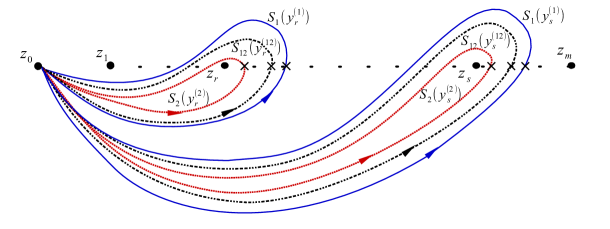
Figure 1: Nested non-intersecting and non-self-intersecting multi-contours for integration over screening currents associated with different vertex operators. The multi-contours around a puncture and which are associated with a particular screening charge are depicted collectively by one loop.

The functions ${W}_{\mathbf{{n_{m},\ldots,n_{1}}}}^{\alpha_{m},\ldots,\alpha_{1}}$ do not by themselves represent conformal blocks, as is easily seen as follows. The commutators between screening currents $S_{i}(z)$ and the generators of the $\mathcal{W}_{3}$-algebra are total derivatives with respect to the variable $z$. When the screening currents $S_{i}(z)$ are integrated over open contours as depicted in Figure 1, one will therefore find boundary terms in the commutators between screening charges and the generators of the $\mathcal{W}_{3}$-algebra supported at the base-point $z_{0}$. The boundary terms will spoil the validity of the Ward identities for the $\mathcal{W}_{3}$-algebra, in general.

However, we will see that the boundary terms all cancel for specific choices of the coefficients $C$ in (3.1). Representing compositions of chiral vertex operators in the form (3.1) is useful since both the problem to find the coefficients $C$ in (3.1) and the calculation of monodromies will be shown to reduce to purely algebraic problems in quantum group theory. In order to explain this relation we shall begin by collecting the definitions and notations concerning the quantum group $\mathcal{U}_{q}({\mathfrak{s}}{\mathfrak{l}}_{3})$ relevant for our goals.

3.2 Quantum group background

The quantum group $\mathcal{U}=\mathcal{U}_{q}({\mathfrak{s}}{\mathfrak{l}}_{N})$ is a Hopf algebra, generated as an associative algebra over $\mathbb{C}(q)$ by ${\mathsf{e}}_{i}$, ${\mathsf{f}}_{i}$ and ${\mathsf{k}}^{\pm}_{i}$ for $i=1,\ldots,N-1$ which satisfy the relations

$$[{\mathsf{e}}_{i},{\mathsf{f}}_{j}]=\delta_{ij}\frac{{\mathsf{k}}_{i}-{\mathsf{k}}_{i}^{-1}}{{q}-{q}^{-1}},\qquad\begin{aligned} &{\mathsf{k}}_{i}^{\pm}{\mathsf{e}}_{j}={q}^{\pm\kappa_{ij}}{\mathsf{e}}_{j}{\mathsf{k}}_{i}^{\pm}~{},\\ &{\mathsf{k}}_{i}^{\pm}{\mathsf{f}}_{j}={q}^{\mp\kappa_{ij}}{\mathsf{f}}_{j}{\mathsf{k}}_{i}^{\pm}~{}\end{aligned}$$ (3.5)

for $i=1,\ldots,N-1$ and where $\kappa$ is the ${\mathfrak{s}}{\mathfrak{l}}_{N}$ Cartan matrix $\kappa_{ij}=2\delta_{ij}-\delta_{i+1,j}-\delta_{i,j+1}~{}.$ The Serre relations are

$${\mathsf{e}}_{i}^{2}{\mathsf{e}}_{j}-({q}+{q}^{-1}){\mathsf{e}}_{i}{\mathsf{e}}_{j}{\mathsf{e}}_{i}+{\mathsf{e}}_{j}{\mathsf{e}}_{i}^{2}=0~{},\quad{\mathsf{f}}_{i}^{2}{\mathsf{f}}_{j}-({q}+{q}^{-1}){\mathsf{f}}_{i}{\mathsf{f}}_{j}{\mathsf{f}}_{i}+{\mathsf{f}}_{j}{\mathsf{f}}_{i}^{2}=0~{},$$ (3.6)

with $|i-j|=1$. Let us now restrict to the case $N=3$. Defining

$${\mathsf{e}}_{12}={\mathsf{e}}_{1}{\mathsf{e}}_{2}-{q}{\mathsf{e}}_{2}{\mathsf{e}}_{1}~{},\qquad{\mathsf{f}}_{12}={\mathsf{f}}_{1}{\mathsf{f}}_{2}-{q}{\mathsf{f}}_{2}{\mathsf{f}}_{1}~{},$$ (3.7)

it follows from the Serre relations that

$${\mathsf{e}}_{1}{\mathsf{e}}_{12} = {q}^{-1}{\mathsf{e}}_{12}{\mathsf{e}}_{1}~{},\qquad{\mathsf{e}}_{2}{\mathsf{e}}_{12}={q}{\mathsf{e}}_{12}{\mathsf{e}}_{2}~{},$$ (3.8)

$${\mathsf{f}}_{1}{\mathsf{f}}_{12} = {q}^{-1}{\mathsf{f}}_{12}{\mathsf{f}}_{1}~{},\qquad{\mathsf{f}}_{2}{\mathsf{f}}_{12}={q}{\mathsf{f}}_{12}{\mathsf{f}}_{2}~{}.$$ (3.9)

Using these relations it is possible to show that arbitrary monomials formed out of the basic generators ${\mathsf{f}}_{i}$, $i=1,2$ can be represented as linear combinations of the ordered monomials ${\mathsf{f}}_{1}^{n_{1}}{\mathsf{f}}_{12}^{n_{12}}{\mathsf{f}}_{2}^{n_{2}}$ with $(n_{1},n_{12},n_{2})\in\mathbb{N}^{3}$.

3.2.1 Representations

The irreducible highest weight representation of $\mathcal{U}_{q}({\mathfrak{s}}{\mathfrak{l}}_{3})$ with highest weight $\lambda$ will be denoted by $\mathcal{R}_{\lambda}$. The highest weight vector $v_{\lambda}\in\mathcal{R}_{\lambda}$ is annihilated by the generators ${\mathsf{e}}_{i}$, ${\mathsf{e}}_{i}v_{\lambda}=0$. The action of ${\mathsf{k}}_{i}$ is

$${\mathsf{k}}_{i}v_{\lambda}={q}^{(e_{i},\lambda)}v_{\lambda}~{}.$$ (3.10)

The representations $\mathcal{R}_{\lambda}$ are irreducible for generic weights $\lambda$. We call a weight $\lambda$ generic if it is not the highest weight of a finite-dimensional highest weight representation of ${\mathfrak{s}}{\mathfrak{l}}_{3}$. We will use a basis for the $\mathcal{U}_{q}({\mathfrak{s}}{\mathfrak{l}}_{3})$ Verma module $\mathcal{R}_{\lambda}$ which consists of the following vectors

$$e_{\mathbf{{n}}}^{\lambda}={\mathsf{f}}_{1}^{n_{1}}{\mathsf{f}}_{12}^{n}{\mathsf{f}}_{2}^{n_{2}}v_{\lambda}~{},\qquad\mathbf{{n}}=(n_{1},n,n_{2})~{}.$$ (3.11)

The vector $e_{\mathbf{{n}}}^{\lambda}$ has weight

$$\nu=\nu(\lambda,{\mathbf{{n}}})=\lambda-(n+n_{1})e_{1}-(n+n_{2})e_{2}~{}.$$ (3.12)

It will sometimes be useful to parameterise the labels $\mathbf{{n}}=(n_{1},n,n_{2})$ in terms of another pair of data $\mathbf{{n}}=[\delta,n]$ consisting of the shift of weights $\delta=-s_{1}e_{1}-s_{2}e_{2}$ together with a multiplicity label $n$ such that $s_{1}=n_{1}+n$ and $s_{2}=n_{2}+n$. For a fixed weight $\nu=\lambda+\delta$ parameterised by positive integers $s_{1}$ and $s_{2}$, one can only have finitely many values of $n$ between $0$ and $d_{\nu}-1=\mathrm{min}(s_{1},s_{2})$. The multiplicity space of a weight $\nu$ has dimension $d_{\nu}$ and will be denoted by $\mathcal{M}^{\nu}_{\lambda}$.

The action of the generators $x$ of $\mathcal{U}_{q}({\mathfrak{s}}{\mathfrak{l}}_{3})$ is represented in the basis (3.11) by the matrices $R_{(x),\mathbf{n}}^{\lambda,\mathbf{n}^{\prime}}$ defined by

$$\pi_{\lambda}(x)e_{\mathbf{{n}}}^{\lambda}=\sum_{\mathbf{{n}}^{\prime}}R_{(x),\mathbf{n}}^{\lambda,\mathbf{n}^{\prime}}e_{\mathbf{{n}}^{\prime}}^{\lambda}.$$ (3.13)

Tables for the matrix elements of $R_{(x),\mathbf{n}}^{\lambda,\mathbf{n}^{\prime}}$ for $x={\mathsf{e}}_{i},{\mathsf{f}}_{i}$ can be found in appendix A. Here we will only note the following important feature concerning the dependence on the multiplicity labels $k$. The action of $\pi_{\lambda}(x)$ on the basis vector $e_{\mathbf{{n}}}^{\lambda}$ can for $x={\mathsf{e}}_{i},{\mathsf{f}}_{i}$, $i=1,2$, be represented in the following form

$$\pi_{\lambda}({\mathsf{e}}_{i})e_{[\delta,k]}^{\lambda} =E_{i}(\lambda,\delta,u_{k})\,e_{[\delta+e_{i},k]}^{\lambda}+E_{i}^{\prime}(\lambda,\delta,u_{k})\,\mathsf{v}^{-1}\,e_{[\delta+e_{i},k]}^{\lambda}~{},$$ (3.14)

$$\pi_{\lambda}({\mathsf{f}}_{i})e_{[\delta,k]}^{\lambda} =F_{i}(\lambda,\delta,u_{k})\,e_{[\delta-e_{i},k]}^{\lambda}+F_{i}^{\prime}(\lambda,\delta,u_{k})\,\mathsf{v}^{+1}\,e_{[\delta-e_{i},k]}^{\lambda}~{},$$

where $u_{k}=q^{-2k}$, $\mathsf{v}e_{[\delta,k]}^{\lambda}=q^{-k}e_{[\delta,k+1]}^{\lambda}$, and the coefficient functions $E_{i}$, $E_{i}^{\prime}$, $F_{i}$ and $F_{i}^{\prime}$ are Laurent polynomials in the variable $u_{k}$. This simple feature will play a crucial role for us in the following.

Apart from the representations associated to generic weights $\lambda$ we will be interested in particular in the fundamental representation generated from the highest weight vector $v_{\omega_{1}}$ and having a basis $\{v_{\omega_{1}},{\mathsf{f}}_{1}v_{\omega_{1}},{\mathsf{f}}_{12}v_{\omega_{1}}\}$.

3.2.2 Tensor products of representations

The coproduct $\Delta$ of $\mathcal{U}_{q}({\mathfrak{s}}{\mathfrak{l}}_{3})$ is defined by

$$\Delta({\mathsf{e}}_{i})={\mathsf{k}}_{i}\otimes{\mathsf{e}}_{i}+{\mathsf{e}}_{i}\otimes 1~{},\quad\Delta({\mathsf{f}}_{i})={\mathsf{f}}_{i}\otimes{\mathsf{k}}_{i}^{-1}+1\otimes{\mathsf{f}}_{i}~{},\quad\Delta({\mathsf{k}}_{i})={\mathsf{k}}_{i}\otimes{\mathsf{k}}_{i}.$$ (3.15)

The coproduct is an algebra homomorphism, so equations (3.15) imply, for example,

$$\Delta({\mathsf{e}}_{12}) = {\mathsf{k}}_{1}{\mathsf{k}}_{2}\otimes{\mathsf{e}}_{12}+{\mathsf{e}}_{12}\otimes 1+(q^{-1}-q){\mathsf{e}}_{2}{\mathsf{k}}_{1}\otimes{\mathsf{e}}_{1}~{}$$

$$\Delta({\mathsf{f}}_{12}) = {\mathsf{f}}_{12}\otimes{\mathsf{k}}_{1}^{-1}{\mathsf{k}}_{2}^{-1}+1\otimes{\mathsf{e}}_{12}+(q^{-1}-q){\mathsf{f}}_{1}\otimes{\mathsf{f}}_{2}{\mathsf{k}}_{1}^{-1}~{}.$$ (3.16)

The Clebsch-Gordan (CG) maps describe the embedding of irreducible representations into tensor products of representations. In the case of the highest weight representations introduced above, one may represent the CG maps $\mathsf{C}^{\lambda_{3}}_{\lambda_{1}\lambda_{2}}:\mathcal{R}_{\lambda_{3}}\rightarrow\mathcal{R}_{\lambda_{1}}\otimes\mathcal{R}_{\lambda_{2}}$ in the form

$$e^{\lambda_{3}}_{\mathbf{{n}}_{3}}(\lambda_{2},\lambda_{1})=\sum_{\begin{subarray}{c}\mathbf{{n}}_{2},\mathbf{{n}}_{1}\\ \nu_{3}=\nu_{2}+\nu_{1}\end{subarray}}\left(\begin{smallmatrix}\lambda_{3}\\ \mathbf{{n}}_{3}\end{smallmatrix}\middle|\begin{smallmatrix}\lambda_{2}&\lambda_{1}\\ \mathbf{{n}}_{2}&\mathbf{{n}}_{1}\end{smallmatrix}\right)e^{\lambda_{1}}_{\mathbf{{n}}_{1}}\otimes e^{\lambda_{2}}_{\mathbf{{n}}_{2}}~{},$$ (3.17)

Here and below we use the notation $\nu_{i}=\nu_{i}(\lambda_{i},\mathbf{{n}}_{i})$ with $\nu(\lambda,{\mathbf{{n}}})$ defined in (3.12).

A set of equations for the Clebsch-Gordan coefficients (CGC) $\left(\begin{smallmatrix}\lambda_{3}\\ \mathbf{{n}}_{3}\end{smallmatrix}\middle|\begin{smallmatrix}\lambda_{2}&\lambda_{1}\\ \mathbf{{n}}_{2}&\mathbf{{n}}_{1}\end{smallmatrix}\right)$ follows from the intertwining property

$$\Delta(x)e_{\mathbf{n}_{3}}^{\lambda_{3}}(\lambda_{2},\lambda_{1})=\sum_{\mathbf{n}^{\prime}_{3}}R_{(x),\mathbf{n}_{3}}^{\lambda_{3},\mathbf{n}^{\prime}_{3}}e_{\mathbf{n}_{3}^{\prime}}^{\lambda_{3}}(\lambda_{2},\lambda_{1})~{},$$ (3.18)

for any element $x\in\mathcal{U}_{q}({\mathfrak{s}}{\mathfrak{l}}_{3})$. When $x={\mathsf{e}}_{i}\in\{{\mathsf{e}}_{1},{\mathsf{e}}_{2}\}$ and $\mathbf{n}_{3}=0$, this equation implies that for every fixed pair $(\mathbf{n}_{1},\mathbf{n}_{2})$

$$0=\sum_{\mathbf{{n}}^{\prime}_{2}}\big{(}\begin{smallmatrix}\lambda_{3}\\ 0\end{smallmatrix}\big{|}\begin{smallmatrix}\lambda_{2}&\lambda_{1}\\ \mathbf{{n}}^{\prime}_{2}&\mathbf{{n}}_{1}\end{smallmatrix}\big{)}{q}^{(e_{i},\nu_{1})}R_{({\mathsf{e}}_{i}),\mathbf{{n}}^{\prime}_{2}}^{\lambda_{2},\mathbf{{n}}_{2}}+\sum_{\mathbf{{n}}^{\prime}_{1}}\big{(}\begin{smallmatrix}\lambda_{3}\\ 0\end{smallmatrix}\big{|}\begin{smallmatrix}\lambda_{2}&\lambda_{1}\\ \mathbf{{n}}_{2}&\mathbf{{n}}^{\prime}_{1}\end{smallmatrix}\big{)}R_{({\mathsf{e}}_{i}),\mathbf{{n}}^{\prime}_{1}}^{\lambda_{1},\mathbf{{n}}_{1}}$$ (3.19)

Equations (3.19) can be regarded as a set of recursion relations. For generic values of $\lambda_{i}$, $i=1,2,3$ one can show that these equations determine $\left(\begin{smallmatrix}\lambda_{3}\\ 0\end{smallmatrix}\middle|\begin{smallmatrix}\lambda_{2}&\lambda_{1}\\ \mathbf{{n}}_{2}&\mathbf{{n}}_{1}\end{smallmatrix}\right)$ uniquely in terms of $\left(\begin{smallmatrix}\lambda_{3}\\ 0\end{smallmatrix}\middle|\begin{smallmatrix}\lambda_{2}&\lambda_{1}\\ \mathbf{{n}}_{2}&0\end{smallmatrix}\right)$. Indeed, it is not hard to see (see Appendix B for further details) that one can use equations (3.19) to derive a recursion relation expressing $\left(\begin{smallmatrix}\lambda_{3}\\ 0\end{smallmatrix}\middle|\begin{smallmatrix}\lambda_{2}&\lambda_{1}\\ \mathbf{{n}}_{2}&\mathbf{{n}}_{1}\end{smallmatrix}\right)$ with $\mathbf{{n}}_{1}=[-s_{1}e_{1}-s_{2}e_{2},k_{1}]$ in terms of the CGC $\left(\begin{smallmatrix}\lambda_{3}\\ 0\end{smallmatrix}\middle|\begin{smallmatrix}\lambda_{2}&\lambda_{1}\\ \mathbf{{m}}_{2}&\mathbf{{m}}_{1}\end{smallmatrix}\right)$ having $\mathbf{{m}}_{1}=[-s_{1}^{\prime}e_{1}-s_{2}^{\prime}e_{2},k_{1}^{\prime}]$ with $s_{1}^{\prime}+s_{2}^{\prime}=s_{1}+s_{2}-1$.

The value of $\left(\begin{smallmatrix}\lambda_{3}\\ 0\end{smallmatrix}\middle|\begin{smallmatrix}\lambda_{2}&\lambda_{1}\\ \mathbf{{n}}_{2}&0\end{smallmatrix}\right)$ is not further constrained by (3.19). A basis for the space of CG maps $\mathsf{C}^{\lambda_{3}}_{\lambda_{1}\lambda_{2}}$ is therefore obtained from the CGC $\left(\begin{smallmatrix}\lambda_{3}\\ \mathbf{{n}}_{3}\end{smallmatrix}\middle|\begin{smallmatrix}\lambda_{2}&\lambda_{1}\\ \mathbf{{n}}_{2}&\mathbf{{n}}_{1}\end{smallmatrix}\right)_{k}$ characterised by the property that

$$\left(\begin{smallmatrix}\lambda_{3}\\ 0\end{smallmatrix}\middle|\begin{smallmatrix}\lambda_{2}&\lambda_{1}\\ \mathbf{{n}}_{2}&0\end{smallmatrix}\right)_{k}=\delta_{k,k_{2}},\quad\text{if}\quad\mathbf{{n}}_{2}=[\delta_{2},k_{2}],\quad\delta_{2}=\lambda_{3}-\lambda_{1}-\lambda_{2}.$$ (3.20)

As $k_{2}$ can only take a finite set of values determined by $\delta_{2}$ we see that the coefficients $\left(\begin{smallmatrix}\lambda_{3}\\ \mathbf{{n}}_{3}\end{smallmatrix}\middle|\begin{smallmatrix}\lambda_{2}&\lambda_{1}\\ \mathbf{{n}}_{2}&\mathbf{{n}}_{1}\end{smallmatrix}\right)_{k}$ define a basis for the space of CG maps. For generic weights $\lambda_{1}$, $\lambda_{2}$, $\lambda_{3}$ there is an isomorphism between the space of CG maps and the subspace with weight $\lambda_{3}-\lambda_{1}$ within $\mathcal{R}_{\lambda_{2}}$, or equivalently the subspace with weight $\lambda_{3}-\lambda_{2}$ within $\mathcal{R}_{\lambda_{1}}$.

It will be important to keep in mind that the $\left(\begin{smallmatrix}\lambda_{3}\\ 0\end{smallmatrix}\middle|\begin{smallmatrix}\lambda_{2}&\lambda_{1}\\ \mathbf{{n}}_{2}&\mathbf{{n}}_{1}\end{smallmatrix}\right)_{k}$ defined using (3.20) depend on the multiplicity labels only through the matrix elements $R_{({\mathsf{e}}_{i}),\mathbf{{n}}^{\prime}}^{\lambda,\mathbf{{n}}}$. The features concerning the dependence of $R_{({\mathsf{e}}_{i}),\mathbf{{n}}^{\prime}}^{\lambda,\mathbf{{n}}}$ on the multiplicity labels observed in (3.14) will be inherited.

Note furthermore that the recursive procedure determining the CGC $\left(\begin{smallmatrix}\lambda_{3}\\ 0\end{smallmatrix}\middle|\begin{smallmatrix}\lambda_{2}&\lambda_{1}\\ \mathbf{{n}}_{2}&\mathbf{{n}}_{1}\end{smallmatrix}\right)_{k}$ proceeds by induction in $s=s_{1}+s_{2}$ if $\mathbf{{n}}_{1}=[-s_{1}e_{1}-s_{2}e_{2},k_{1}]$. In each step one generically increases the range of values for the multiplicity label $k_{2}$ in $\mathbf{{n}}_{2}=[\delta_{2},k_{2}]$ with non-vanishing $\left(\begin{smallmatrix}\lambda_{3}\\ 0\end{smallmatrix}\middle|\begin{smallmatrix}\lambda_{2}&\lambda_{1}\\ \mathbf{{n}}_{2}&\mathbf{{n}}_{1}\end{smallmatrix}\right)_{k}$ by one unit. In the case $\mathbf{{n}}_{1}=[-s_{1}e_{1}-s_{2}e_{2},k_{1}]$ with $s_{1}+s_{2}\leq 2$, for example, we find non-vanishing $\left(\begin{smallmatrix}\lambda_{3}\\ 0\end{smallmatrix}\middle|\begin{smallmatrix}\lambda_{2}&\lambda_{1}\\ \mathbf{{n}}_{2}&\mathbf{{n}}_{1}\end{smallmatrix}\right)_{k}$ only for $k-2\leq k_{2}\leq k$. Further details are given in Appendix B.

3.2.3 Iterated Clebsch-Gordan maps

Families of intertwining maps $\mathsf{C}:\bigotimes_{l=1}^{n-1}\mathcal{R}_{l}\rightarrow\bar{\mathcal{R}}_{n}$ can be constructed as compositions of the Clebsch-Gordan maps introduced in Section 3.2.2. For $m=3$, for example, one may consider linear combinations of the form

$$e^{\lambda_{4}}_{\mathbf{{n}}_{4}}(\lambda_{3},\lambda_{2},\lambda_{1})=\sum_{\begin{subarray}{c}\mathbf{n}_{3},\mathbf{n}_{2},\mathbf{n}_{1}\\ \nu_{4}=\nu_{1}+\nu_{2}+\nu_{3}\end{subarray}}\left(\begin{smallmatrix}\lambda_{4}\\ \mathbf{{n}}_{4}\end{smallmatrix}\middle|\begin{smallmatrix}\lambda_{3}&\lambda_{2}&\lambda_{1}\\ \mathbf{{n}}_{3}&\mathbf{{n}}_{2}&\mathbf{{n}}_{1}\end{smallmatrix}\right)e_{\mathbf{n}_{1}}^{\lambda_{1}}\otimes e_{\mathbf{n}_{2}}^{\lambda_{2}}\otimes e_{\mathbf{n}_{3}}^{\lambda_{3}},$$ (3.21)

One may argue in the same way as before that the coefficients in (3.21) are uniquely determined in terms of the particular values for $\mathbf{{n}}_{4}=0$ and $\mathbf{{n}}_{1}=0$. The space $\mathrm{CG}(\lambda_{4}|\lambda_{3}\lambda_{2}\lambda_{1})$ of Clebsch-Gordan maps is therefore isomorphic to the subspace denoted by $\mathcal{R}_{\lambda_{3},\lambda_{2}}^{\lambda_{4}-\lambda_{1}}$ in $\mathcal{R}_{\lambda_{3}}\otimes\mathcal{R}_{\lambda_{2}}$ with total weight $\lambda_{4}-\lambda_{1}$. It is then easy to see that a basis for this space is provided by the composition of Clebsch-Gordan maps,

$$\left(\begin{smallmatrix}\lambda_{4}\\ 0\end{smallmatrix}\middle|\begin{smallmatrix}\lambda_{3}&\lambda_{2}&\lambda_{1}\\ \mathbf{{n}}_{3}&\mathbf{{n}}_{2}&0\end{smallmatrix}\right)_{k_{3},k_{2}}^{\lambda_{12}}=\sum_{\begin{subarray}{c}\mathbf{n}_{12}\\ \nu_{12}=\lambda_{1}+\nu_{2}\end{subarray}}\left(\begin{smallmatrix}\lambda_{4}\\ 0\end{smallmatrix}\middle|\begin{smallmatrix}\lambda_{3}&\lambda_{12}\\ \mathbf{{n}}_{3}&\mathbf{{n}}_{12}\end{smallmatrix}\right)_{k_{3}}\big{(}\begin{smallmatrix}\lambda_{12}\\ \mathbf{{n}}_{12}\end{smallmatrix}\big{|}\begin{smallmatrix}\lambda_{2}&\lambda_{1}\\ \mathbf{{n}}_{2}&0\end{smallmatrix}\big{)}_{k_{2}}~{}.$$ (3.22)

The coefficients (3.22) represent the matrix elements of a map $\mathsf{D}^{\lambda_{4}}_{\lambda_{3}\lambda_{2}\lambda_{1}}$ from $\mathrm{CG}(\lambda_{4}|\lambda_{3}\lambda_{2}\lambda_{1})$ into $\mathcal{R}_{\lambda_{3},\lambda_{2}}^{\lambda_{4}-\lambda_{1}}$.

3.2.4 R-matrix

The universal R-matrix is an invertible element $\mathsf{R}\in\mathcal{U}_{q}({\mathfrak{s}}{\mathfrak{l}}_{N})\otimes\mathcal{U}_{q}({\mathfrak{s}}{\mathfrak{l}}_{N})$ with the property

$$\mathsf{R}\Delta(x)\mathsf{R}^{-1}=(\mathsf{P}\circ\Delta)(x)~{},\qquad x\in\mathcal{U}_{q}({\mathfrak{s}}{\mathfrak{l}}_{N})~{},$$ (3.23)

where $\mathsf{P}\in\mathcal{U}_{q}({\mathfrak{s}}{\mathfrak{l}}_{N})\otimes\mathcal{U}_{q}({\mathfrak{s}}{\mathfrak{l}}_{N})$ is the permutation that acts as $\mathsf{P}(x\otimes y)=y\otimes x$. It satisfies the Yang-Baxter equation $\mathsf{R}_{12}\mathsf{R}_{13}\mathsf{R}_{23}=\mathsf{R}_{23}\mathsf{R}_{13}\mathsf{R}_{12}$ and the action of the coproduct on it is

$$(\Delta\otimes 1)\mathsf{R}=\mathsf{R}_{13}\mathsf{R}_{23}~{},\qquad(1\otimes\Delta)\mathsf{R}=\mathsf{R}_{13}\mathsf{R}_{12}~{}.$$ (3.24)

It can be shown that the conditions (3.23) have a unique solution of the form $\mathsf{R}=q^{t}\bar{\mathsf{R}}$ with $t=\sum_{ij}(\kappa_{ij}^{-1})\mathsf{h}_{i}\otimes\mathsf{h}_{j}$, with $\kappa_{ij}$ being the Cartan matrix, if ${\mathsf{k}}_{i}={q}^{\mathsf{h}_{i}}$, and

$$\bar{\mathsf{R}}=1+({q}-{q}^{-1})({\mathsf{e}}_{1}\otimes{\mathsf{f}}_{1}+{\mathsf{e}}_{2}\otimes{\mathsf{f}}_{2}-{q}^{-1}{\mathsf{e}}_{12}\otimes{\mathsf{f}}_{12})+({q}-{q}^{-1})^{2}{\mathsf{e}}_{2}{\mathsf{e}}_{1}\otimes{\mathsf{f}}_{2}{\mathsf{f}}_{1}+\dots~{}~{}~{}~{}~{}$$ (3.25)

The omitted terms in the expression (3.25) are of higher order in ${\mathsf{e}}_{i}$, $i=1,2$.

The universal R-matrix is related to the braid matrices $\mathsf{B}_{\lambda_{1}\lambda_{2}}:{\mathcal{R}}_{\lambda_{1}}\otimes{\mathcal{R}}_{\lambda_{2}}\to{\mathcal{R}}_{\lambda_{2}}\otimes{\mathcal{R}}_{\lambda_{1}}$ through

$$\mathsf{B}_{\lambda_{1}\lambda_{2}}=\mathsf{P}\circ\mathsf{r}_{\lambda_{1}\lambda_{2}},\quad\text{where}\quad\mathsf{r}_{\lambda_{1}\lambda_{2}}=(\pi_{\lambda_{1}}\otimes\pi_{\lambda_{2}})(\mathsf{R})$$ (3.26)

is the evaluation of the universal R-matrix in the tensor product of representations ${\mathcal{R}}_{\lambda_{1}}\otimes{\mathcal{R}}_{\lambda_{2}}$ and $P$ is the permutation of tensor factors. Our notation for the matrix elements of $\mathsf{B}_{\lambda_{1}\lambda_{2}}$ is defined such that

$$\mathsf{B}_{\lambda_{1}\lambda_{2}}\,e_{\mathbf{{n}}_{1}}^{\lambda_{1}}\otimes e_{\mathbf{{n}}_{2}}^{\lambda_{2}}=\sum_{\mathbf{m}_{1},\mathbf{m}_{2}}(B_{\lambda_{1}\lambda_{2}})_{\mathbf{n}_{1}}^{\mathbf{m}_{1}}{}^{\mathbf{m}_{2}}_{\mathbf{n}_{2}}e_{\mathbf{{m}}_{2}}^{\lambda_{2}}\otimes e_{\mathbf{{m}}_{1}}^{\lambda_{1}}~{}.$$ (3.27)

3.3 Braiding of screened vertex operators

The spaces of functions generated by the functions ${W}_{\mathbf{{n_{m},\ldots,n_{1}}}}^{\alpha_{m},\ldots,\alpha_{1}}(z_{m},\ldots,z_{1})$ introduced in (3.2) carry a natural action of the braid group which turns out to be related to the representation of the braid group on tensor products of quantum group representations. We will now briefly explain this first crucial link between quantum group theory and free field representation to be used in this paper.

Let us consider ${W}_{\mathbf{{n_{2}n_{1}}}}^{\alpha_{2}\alpha_{1}}(z_{2},z_{1})$ defined using the contours from Figure 1. The braiding operations are defined using the analytic continuation of this function with respect to $z_{2}$ and $z_{1}$ along a path exchanging their positions. This analytic continuation can be defined by integrating along suitably deformed contours as indicated in Figure 2.

Figure 2: Braiding of two generic multi-contours. The collections of contours associated with general products of screening charges are depicted here as simple loops around the punctures.

By means of contour deformations one can represent the result of this operation as a linear combination of integrals over the contours introduced in Figure 1.

This can be done by the following recursive procedure. In a first sequence of steps, performed in an induction over $\mathbf{{n}}_{2}=(n_{2,1},n_{2,21},n_{2,2})$ one may deform the contours on the right of Figure 2 into linear combinations of the contours depicted in Figure 3 .

Figure 3: A set of auxiliary contours for the braiding calculation.

The induction step is indicated in Figure 4.

Figure 4: Deformation of the outermost of the contours encircling $z_{2}$ representing a step in the passage to linear combinations of the contours depicted in Figure 3, where $\mathbf{s}_{1}=(1,0,0)$.

In a second sequence of steps one may then deform the contours surrounding both $z_{1}$ and $z_{2}$ in Figure 3 into a linear combination of contours surrounding only $z_{1}$ or $z_{2}$ at a time. The result of this procedure can be represented as linear combination of the original contours introduced in Figure 1, leading to a relation of the form

$$\mathcal{B}\big{(}W_{\mathbf{n}_{2}\mathbf{n}_{1}}^{\alpha_{2}\alpha_{1}}(z_{2},z_{1})\big{)}=\sum_{\mathbf{m}_{1},\mathbf{m}_{2}}(b_{\alpha_{1}\alpha_{2}})_{\mathbf{n}_{1}}^{\mathbf{m}_{1}}{}^{\mathbf{m}_{2}}_{\mathbf{n}_{2}}W_{\mathbf{m}_{2}\mathbf{m}_{1}}^{\alpha_{2}\alpha_{1}}(z_{1},z_{2})$$ (3.28)

We will explain in more detail in Appendix C below how such computations can be done and calculate the matrix elements of $b_{\alpha_{1}\alpha_{2}}$ for the important special case where $\alpha_{2}=-b\omega_{1}$ with $\alpha_{1}$ generic. The result can be compared to the action of the braid group on tensor products of quantum group representations defined in (3.27). It turns out that the matrix $b_{\alpha_{1}\alpha_{2}}$ appearing in (3.28) coincides with the matrix $B_{\lambda_{1}\lambda_{2}}$ in (3.27) provided that $\lambda_{l}=-\alpha_{l}/b$ for $l=1,2$. This result can easily be generalised to the cases where $\alpha_{2}=-b\lambda_{2}$ with $\lambda_{2}$ being the weight of any finite-dimensional representation of $\mathcal{U}_{q}({\mathfrak{s}}{\mathfrak{l}}_{3})$ by noting that any finite-dimensional representation of $\mathcal{U}_{q}({\mathfrak{s}}{\mathfrak{l}}_{3})$ appears in the iterated tensor products of fundamental representations, and that the co-product of the quantum group has a simple representation in terms of the free field representation, as indicated in Figure 5 below.

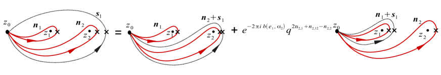
Figure 5: Decomposition of a simple contour associated with the root $e_{1}$ around two punctures into contours enclosing only one of the punctures. This decomposition represents the co-product $\Delta({\mathsf{f}}_{1})=1\otimes{\mathsf{f}}_{i}+{\mathsf{f}}_{1}\otimes{\mathsf{k}}_{1}^{-1}$.

As representations of the braid group one may therefore identify the vector spaces generated by the functions ${W}_{\mathbf{{n}}_{m},\ldots,\mathbf{{n}}_{1}}^{\alpha_{m},\ldots,\alpha_{1}}(z_{m},\ldots,z_{1})$ with the tensor product of quantum group representations $\bigotimes_{l=1}^{m}\mathcal{R}_{\lambda_{l}}$ assuming that the weights are related as $\lambda_{l}=-\alpha_{l}/b$, $l=1,\dots,m$.

3.4 Construction of conformal blocks

We had noted above that the functions ${W}_{\mathbf{{n_{m},\ldots,n_{1}}}}^{\alpha_{m},\ldots,\alpha_{1}}(z_{m},\ldots,z_{1})$ are not the objects we are ultimately interested in. They do not satisfy the Ward identities for the $\mathcal{W}_{3}$-algebra characterising the conformal blocks. It turns out, however, that there exist suitable linear combinations of the form (3.1) which will indeed represent conformal blocks. We are now going to argue that this will be the case if the coefficients $C$ in (3.1) are the matrix elements of the Clebsch-Gordan maps describing the embedding of the irreducible representation with weight $\lambda_{\infty}=-b^{-1}\alpha_{\infty}$ into the tensor product $\bigotimes_{l=1}^{m}\mathcal{R}_{\lambda_{l}}$. For $m=3$, for example, one may get expressions of the following form

$$\langle v_{\infty},V^{\rho_{3}}_{k_{3}}(z_{3})V^{\rho_{2}}_{k_{2}}(z_{2}){\mathfrak{e}}_{\alpha_{1}}\rangle=$$ (3.29)

$$\qquad\qquad=\sum_{\begin{subarray}{c}\mathbf{n}_{3},\mathbf{n}_{2},\mathbf{n}_{1},\mathbf{n}_{12}\\ \lambda_{4}=\nu_{12}+\nu_{3}\\ \nu_{12}=\nu_{1}+\nu_{2}\end{subarray}}\left(\begin{smallmatrix}\lambda_{4}\\ 0\end{smallmatrix}\middle|\begin{smallmatrix}\lambda_{3}&\lambda_{12}\\ \mathbf{{n}}_{3}&\mathbf{{n}}_{12}\end{smallmatrix}\right)_{k_{3}}\left(\begin{smallmatrix}\lambda_{12}\\ \mathbf{{n}}_{12}\end{smallmatrix}\middle|\begin{smallmatrix}\lambda_{2}&\lambda_{1}\\ \mathbf{{n}}_{2}&\mathbf{{n}}_{1}\end{smallmatrix}\right)_{k_{2}}{W}_{\mathbf{{n}}_{3},\mathbf{{n}}_{2},\mathbf{{n}}_{1}}^{\alpha_{3},\alpha_{2},\alpha_{1}}(z_{3},z_{2},0),$$

where $\rho_{2}=(\alpha_{12},\alpha_{2},\alpha_{1})$ and $\rho_{3}=(\alpha_{\infty},\alpha_{3},\alpha_{12})$ with $\alpha_{12}=-b\lambda_{12}$. Note that the summations in (3.29) include summations over the multiplicity labels of $\mathbf{{n}}_{3}$, $\mathbf{{n}}_{2}$, $\mathbf{{n}}_{1}$ and $\mathbf{{n}}_{12}$ together with a summation over two out the three weights $\nu_{1}$, $\nu_{2}$ and $\nu_{3}$.

3.4.1 Relation to quantum group theory

In order to see the relation between the problem to find linear combinations of the form (3.1) representing conformal blocks and the Clebsch-Gordan problem one needs to notice that the boundary terms appearing in the commutators of the screening charges with the generators of the algebra $\mathcal{W}_{3}$ turn out to be related to the action of the generators ${\mathsf{e}}_{i}$ on tensor products of quantum group representations defined by means of the co-product. In order to formulate a more precise statement, let us introduce some useful notations. Let

$${V}_{\mathbf{{n}}_{m},\ldots,\mathbf{{n}}_{1}}^{\alpha_{m},\ldots,\alpha_{1}}(z_{m},\ldots,z_{1})=\int_{\check{\Gamma}}d\mathbf{{y}}_{m}\ldots d\mathbf{{y}}_{1}\;\mathbf{{S}}^{\mathbf{{n}}_{m}}_{m}(\mathbf{{y}}_{m})V_{\alpha_{m}}(z_{m})\ldots\mathbf{{S}}^{\mathbf{{n}}_{1}}_{1}(\mathbf{{y}}_{1})V_{\alpha_{1}}(z_{1})$$ (3.30)

be the operator appearing in the matrix elements (3.2) defining the functions ${W}_{\mathbf{{n_{m},\ldots,n_{1}}}}^{\alpha_{m},\ldots,\alpha_{1}}$. The correspondence with vectors in tensor products of quantum group representations observed above can be schematically represented as

$${V}_{\mathbf{{n}}_{m},\ldots,\mathbf{{n}}_{1}}^{\alpha_{m},\ldots,\alpha_{1}}\quad\leftrightarrow\quad e_{\mathbf{n}_{1}}^{\lambda_{1}}\otimes\ldots\otimes e_{\mathbf{n}_{m}}^{\lambda_{m}}~{},$$ (3.31)

allowing us to introduce the notation

$$\big{(}\Delta(x){V}_{\mathbf{{n}}_{m},\ldots,\mathbf{{n}}_{1}}^{\alpha_{m},\ldots,\alpha_{1}}\big{)}(z_{m},\ldots,z_{1})$$ (3.32)

for the vertex operator associated to $\Delta(x)e_{\mathbf{n}_{1}}^{\lambda_{1}}\otimes\ldots\otimes e_{\mathbf{n}_{m}}^{\lambda_{m}}$ for $x\in\mathcal{U}_{q}({\mathfrak{s}}{\mathfrak{l}}_{3})$ via the correspondence (3.31). In the computation of the commutator of the vertex operators ${V}_{\mathbf{{n}}_{m},\ldots,\mathbf{{n}}_{1}}^{\alpha_{m},\ldots,\alpha_{1}}$ with the generators of the algebra $\mathcal{W}_{3}$ one may distinguish terms from the commutators of the screening currents from the terms coming from commutators with other exponential fields. The contribution of the former is then found to be a linear combination of terms which are proportional to $(\Delta({\mathsf{e}}_{i}){V}_{\mathbf{{n}}_{m},\ldots,\mathbf{{n}}_{1}}^{\alpha_{m},\ldots,\alpha_{1}})(z_{m},\ldots,z_{1})$. Considering, for example, the commutator with $L_{-1}$ we find

$$\big{[}\,L_{-1}\,,\,{V}_{\mathbf{{n}}_{m},\ldots,\mathbf{{n}}_{1}}^{\alpha_{m},\ldots,\alpha_{1}}(z_{m},\ldots,z_{1})\,\big{]}=\sum_{l=1}^{m}\partial_{z_{l}}{V}_{\mathbf{{n}}_{m},\ldots,\mathbf{{n}}_{1}}^{\alpha_{m},\ldots,\alpha_{1}}(z_{m},\ldots,z_{1})+(\text{boundary terms}),$$ (3.33)

with boundary terms proportional to $(\Delta(x){V}_{\mathbf{{n}}_{m},\ldots,\mathbf{{n}}_{1}}^{\alpha_{m},\ldots,\alpha_{1}})(z_{m},\ldots,z_{1})$ for

$$x=(q-q^{-1})({\mathsf{k}}_{1}^{-1}{\mathsf{e}}_{1}+{\mathsf{k}}_{2}^{-1}{\mathsf{e}}_{2}).$$ (3.34)

The derivation of these statements is outlined in Appendix D. We conclude that the boundary terms in the commutators with generators of the algebra $\mathcal{W}_{3}$ will vanish if the coefficients $C$ in (3.1) are taken to be the expansion coefficients of the images of highest weight vectors under the CG maps.

3.4.2 Independence of the choice of base-point

The linear combinations (3.1) representing conformal blocks do not depend on the position of the base point $z_{0}$ indicated in Figure 1. Indeed, the derivative of ${W}_{\mathbf{{n_{m},\ldots,n_{1}}}}^{\alpha_{m},\ldots,\alpha_{1}}$ with respect to $z_{0}$ yields boundary terms which cancel in the linear combinations (3.1) by the same arguments as used above.

The independence of $z_{0}$ can be used for our advantage in two ways. One may note, on the one hand, that the expressions for conformal blocks resulting from (3.1) can be replaced by expressions where different base points $z_{0}$ are associated to each individual CG coefficient appearing in expressions like (3.29). In (3.29), for example, one could have a base-point $z_{0}$ for the integrations with screening numbers $\mathbf{n}_{1}$ and $\mathbf{n}_{2}$, and another base-point $z_{0}^{\prime}$ for those with screening numbers $\mathbf{n}_{12}$ and $\mathbf{n}_{3}$, as depicted in Figure 6. In this form it is manifest that the conformal blocks defined via (3.29) factorise into three-point conformal blocks, as they should. This representation furthermore exhibits clearly the relation between the intermediate representation $\mathcal{V}_{\alpha_{12}}$ of the algebra $\mathcal{W}_{3}$ appearing in the conformal blocks on the left side of (3.29) and the intermediate representation $\mathcal{R}_{\lambda_{12}}$ appearing in the Clebsch-Gordan coefficients on the right side of (3.29), with representation labels related by $\alpha_{12}=-b\lambda_{12}$.

Figure 6: Different base points $z_{0}$ and $z_{0}^{\prime}$ associated with different integration contours.

If, furthermore, the components of $\alpha_{1}$ are sufficiently negative, one may simplify the expression (3.29) by taking the limit where the base-point $z_{0}$ used in the definition of the contours approaches $z_{1}$. Taking into account (3.20) the expression (3.29) gets simplified to

$$\langle v_{\infty},V^{\rho_{3}}_{k_{3}}(z_{3})V^{\rho_{2}}_{k_{2}}(z_{2}){\mathfrak{e}}_{\alpha_{1}}\rangle=\sum_{\begin{subarray}{c}\mathbf{n}_{3}\\ \nu_{3}+\nu_{2}=\lambda_{4}-\lambda_{1}\end{subarray}}D_{k_{3}k_{2}}^{\lambda_{12}}\left(\begin{smallmatrix}\lambda_{4}\\ 0\end{smallmatrix}\middle|\begin{smallmatrix}\lambda_{3}&\lambda_{2}&\lambda_{1}\\ \mathbf{{n}}_{3}&\mathbf{{n}}_{2}&0\end{smallmatrix}\right){W}_{\mathbf{{n}}_{3},\mathbf{{n}}_{2},0}^{\alpha_{3},\alpha_{2},\alpha_{1}}(z_{3},z_{2},0),$$ (3.35)

where $\mathbf{{n}}_{2}=[\lambda_{12}-\lambda_{1}-\lambda_{2},k_{2}]$, $\rho_{2}=(\alpha_{12},\alpha_{2},\alpha_{1})$ and $\rho_{3}=(\alpha_{\infty},\alpha_{3},\alpha_{12})$ with $\alpha_{12}=-b\lambda_{12}$. The expression for the coefficients $D_{k_{3},k_{2}}^{\lambda_{12}}$ in (3.35) gets simplified to

$$D_{k_{3},k_{2}}^{\lambda_{12}}\left(\begin{smallmatrix}\lambda_{4}\\ 0\end{smallmatrix}\middle|\begin{smallmatrix}\lambda_{3}&\lambda_{2}&\lambda_{1}\\ \mathbf{{n}}_{3}&\mathbf{{n}}_{2}&0\end{smallmatrix}\right)=\sum_{\begin{subarray}{c}\mathbf{n}_{12}\\ \nu_{12}=\lambda_{4}-\nu_{3}\end{subarray}}\left(\begin{smallmatrix}\lambda_{4}\\ 0\end{smallmatrix}\middle|\begin{smallmatrix}\lambda_{3}&\lambda_{12}\\ \mathbf{{n}}_{3}&\mathbf{{n}}_{12}\end{smallmatrix}\right)_{k_{3}}~{}.$$ (3.36)

We see that sending $z_{0}$ to $z_{1}$ is related to the projection of the tensor product $\bigotimes_{l=1}^{3}\mathcal{R}_{\lambda_{l}}$ onto the subspace $v_{\lambda_{1}}\otimes\bigotimes_{l=2}^{3}\mathcal{R}_{\lambda_{l}}$. This projection obviously commutes with the braiding operation applied to the second and third tensor factors, allowing us to simplify the computations.

It can also be useful to consider the limit where $z_{0}\to z_{2}$. In this case one may use contours supported near the circles around the origin with radius $|z_{2}|$, allowing us represent the CVOs as composite operators of the form $Q_{1}^{n_{1}}(\gamma)Q_{12}^{n_{12}}(\gamma)Q_{2}^{n_{2}}(\gamma)V_{\alpha_{2}}(z_{2})$, with screening charges $Q_{i}(z)=\int_{\gamma}S_{i}(y)$ being defined by integration over $\gamma=\{y\in{\mathbb{C}};|y|=|z_{2}|\}$ for $i=1,12,2$.

4 Computation of monodromies

We will now explain how the connection between free field representation and quantum group theory helps us to compute the representation of monodromies on spaces of conformal blocks. Recall that we are interested in calculating the monodromies of the conformal blocks

$$\mathcal{F}_{k}^{\rho}(y;y_{0})_{\bar{\imath}\imath}=\langle\,{{\mathfrak{e}}}_{\alpha_{3}}\,,\,\bar{D}_{\bar{\imath}}(y_{0})D_{\imath}(y)\,V_{k}^{\rho}(z)\,{\mathfrak{e}}_{\alpha_{1}}\rangle,$$ (4.1)

regarded as function of $y$. The task can be simplified slightly by sending the base-point $y_{0}$ to infinity, reducing the problem to the computation of the monodronies of the four-point conformal blocks

$$\mathcal{G}_{k}^{\rho}(y)_{\imath}=\langle\,v_{\infty}\,,\,D_{\imath}(y)\,V_{k}^{\rho}(z)\,{\mathfrak{e}}_{\alpha_{1}}\rangle,$$ (4.2)

where $v_{\infty}\in{\mathcal{V}}_{\alpha_{4}}$ with $\alpha_{4}$ being related to the variables $\alpha_{3}$ and $\bar{\imath}$ in (4.1) as $\alpha_{4}=\alpha_{3}-bh_{\bar{\imath}}$.

We will therefore consider the space of conformal blocks on the four-punctured sphere $\mathbb{P}^{1}\setminus\{z_{1}=0,z_{2}=z,z_{3}=y,z_{4}=\infty\}$ with representation ${\mathcal{V}}_{\alpha_{r}}$ assigned to $z_{r}$, $r=1,\dots,4$. The free field representation identifies this space with the subspace of $\bigotimes_{l=1}^{3}\mathcal{R}_{\lambda_{l}}$ with weight $\lambda_{4}-\lambda_{1}$, assuming that $\alpha_{r}=-b\lambda_{r}$ for $r=1,\dots,4$.

The fundamental group of $C_{0,3}=\mathbb{P}^{1}\setminus\{0,z,\infty\}$ is generated by the loops $\gamma_{0}$, $\gamma_{z}$, $\gamma_{\infty}$ around $0$, $z$ and $\infty$. Since the loop $\gamma_{0}\circ\gamma_{z}\circ\gamma_{\infty}$ is contractible, it suffices to compute the monodromies along two out of the three loops. The monodromy of the conformal blocks $\mathcal{G}_{k}^{\rho}(y)_{\imath}$ introduced in (4.2) around $\infty$ is a simple diagonal matrix. It will therefore suffice to compute the monodromy of $\mathcal{G}_{k}^{\rho}(y)_{\imath}$ along a loop surrounding $z_{2}=z$. The free field representation introduced above relates this monodromy to

$$(\mathsf{D}^{\lambda_{4}}_{\lambda_{1}\lambda_{2}\lambda_{3}})^{-1}\cdot\mathsf{B}_{\lambda_{3}\lambda_{2}}\cdot\mathsf{B}_{\lambda_{2}\lambda_{3}}\cdot\mathsf{D}^{\lambda_{4}}_{\lambda_{1}\lambda_{2}\lambda_{3}}~{},$$ (4.3)

where $\mathsf{D}$ is the linear operator defined in (3.29), and $\mathsf{B}_{\lambda_{3}\lambda_{2}}:{\mathcal{R}}_{\lambda_{3}}\otimes{\mathcal{R}}_{\lambda_{2}}\to{\mathcal{R}}_{\lambda_{2}}\otimes{\mathcal{R}}_{\lambda_{3}}$ is the braiding operation.

As explained previously, we will mainly be interested in the case where the representation $\mathcal{R}_{\lambda_{3}}$ assigned to $z_{3}=y$ is the fundamental representation, $\lambda_{3}=\omega_{1}$. The simplifications resulting from $\lambda_{3}=\omega_{1}$ will be discussed next.

4.1 Conformal blocks with degenerate fields

In the case $\lambda_{3}=\omega_{1}$ the weight $\lambda_{12}$ in (3.35) can only take the values $\lambda_{\imath}=\lambda_{4}-h_{\imath}$, $\imath=1,2,3$. The expansion (3.35) further simplifies to

$$\langle v_{\infty},D_{\imath}(y)V^{\rho_{2}}_{k}(z){\mathfrak{e}}_{\alpha_{1}}\rangle=\sum_{\jmath=1}^{3}\sum_{\begin{subarray}{c}\mathbf{n}_{2}\\ \lambda_{4}=h_{\jmath}+\nu_{2}+\lambda_{1}\end{subarray}}\!\!D_{k,0}^{\lambda_{\imath}}\big{(}\begin{smallmatrix}\lambda_{4}\\ 0\end{smallmatrix}\big{|}\begin{smallmatrix}\omega_{1}&\lambda_{2}&\lambda_{1}\\ \mathbf{{d}}_{\jmath}&\mathbf{{n}}_{2}&0\end{smallmatrix}\big{)}{W}_{\mathbf{{d}}_{\jmath},\mathbf{{n}}_{2},0}^{-b\omega_{1},\alpha_{2},\alpha_{1}}(y,z,0),$$ (4.4)

where $\mathbf{{d}}_{i}=[\omega_{1}-h_{i},0]$, $i=1,2$, and $\mathbf{{d}}_{3}=[\omega_{1}-h_{3},1]$. One should also remember that $\mathbf{{n}}_{2}$ is fixed as $\mathbf{{n}}_{2}=[\lambda_{12}-\lambda_{1}-\lambda_{2},k]$ through equation (3.20). Taking this constraint into account, we will in the following replace the notation ${W}_{\mathbf{{d}}_{\jmath},\mathbf{{n}}_{2},0}^{-b\omega_{1},\alpha_{2},\alpha_{1}}$ by ${W}_{\jmath,k}^{\alpha_{4},\alpha_{2},\alpha_{1}}$. Noting that $\nu_{12}=\lambda_{4}-h_{\imath}$ one finds that the summation over $\mathbf{{n}}_{12}$ in (3.36) can take only the four possible values $\mathbf{{s}}_{i}=[-e_{i},0]$, $i=1,2$ and $[-e_{12},\epsilon]$, $e_{12}=e_{1}+e_{2}$, $\epsilon\in\{0,1\}$. One may then write (4.4) a bit more concisely in the form

$$\langle v_{\infty},D_{\imath}(y){V}^{\rho}_{k}(z){\mathfrak{e}}_{\alpha_{1}}\rangle=\sum_{\jmath=1}^{3}{D}_{\imath\jmath}(\lambda_{4}){W}_{\jmath,k}^{\alpha_{4},\alpha_{2},\alpha_{1}}(z_{3},z_{2},z_{1}).$$ (4.5)

The remaining coefficients in (4.5) are

$$D_{ii}=1~{},\quad D_{i+1~{}i}=\big{(}\begin{smallmatrix}\lambda_{4}\\ 0\end{smallmatrix}\big{|}\begin{smallmatrix}\omega_{1}&\lambda_{4}-h_{i+1}\\ \mathbf{{d}}_{i}&\mathbf{s}_{i}\end{smallmatrix}\big{)}~{},\quad D_{31}=\sum_{\epsilon=0}^{1}\big{(}\begin{smallmatrix}\lambda_{4}\\ 0\end{smallmatrix}\big{|}\begin{smallmatrix}\omega_{1}&\lambda_{4}-h_{3}\\ 0&[-e_{12},\epsilon]\end{smallmatrix}\big{)}~{}.$$ (4.6)

Using the notation

$$[n]=\frac{1-{q}^{2n}}{1-{q}^{2}}~{}.$$ (4.7)

the non vanishing matrix elements of $D$ can be represented explicitly as

$$\begin{aligned} &D_{21}={q}^{-1}[-(e_{1},\lambda_{4})]^{-1}~{},\\ &D_{32}={q}^{2(e_{2},\lambda_{4})-2}\big{(}[1-(e_{2},\lambda_{4})]-[1+(e_{1},\lambda_{4})]\big{)}\big{(}[(e_{2},\lambda_{4})-1]\mathsf{c}^{(2)}_{\lambda_{4}}\big{)}^{-1}~{},\\ &{D}_{31}={q}^{2(e_{12},\lambda_{4})-1}\left(1-[1-(e_{2},\lambda_{4})]\right)\big{(}[(e_{2},\lambda_{4})-1]\mathsf{c}^{(2)}_{\lambda_{4}}\big{)}^{-1}~{},\end{aligned}$$ (4.8)

$$\mathsf{c}^{(2)}_{\lambda_{4}}={q}^{2+2(e_{1},\lambda_{4})}(1+[1-(e_{12},\lambda_{4})])-(1-{q}^{2})([1-(e_{2},\lambda_{4})]-[1+(e_{1},\lambda_{4})]).$$

The derivation of these expressions is outlined in Appendix B.2.

4.2 Braiding with fundamental representation

The form of the braid relations also simplifies when $\lambda_{2}=\omega_{1}$ or $\lambda_{3}=\omega_{1}$. Let us first consider the case $\lambda_{2}=\omega_{1}$. The braid matrix preserves weight subspaces in the tensor product. Recalling that the only allowed weights in the fundamental representation are $h_{\imath}$, $\imath=1,2,3$ one notes that the subspace in $\mathcal{R}_{\omega_{1}}\otimes\mathcal{R}_{\lambda}$ having fixed total weight $\nu$ is spanned by vectors of the form $e^{\omega_{1}}_{\delta_{\imath}}\otimes e^{\lambda}_{\mathbf{{n}}}$ with weight of $e^{\lambda}_{\mathbf{{n}}}$ being $\nu-h_{\imath}$ for $\imath=1,2,3$. For fixed $\imath$ one gets a subspace of $\mathcal{R}_{\omega_{1}}\otimes\mathcal{R}_{\lambda}$ isomorphic to the multiplicity space $\mathcal{M}^{\nu-h_{\imath}}_{\lambda}$. The projection of the braiding operator $\mathsf{B}_{\omega_{1}\lambda}:\mathcal{R}_{\omega_{1}}\otimes\mathcal{R}_{\lambda}\rightarrow\mathcal{R}_{\lambda}\otimes\mathcal{R}_{\omega_{1}}$ onto a subspace of total weight $\nu$ can be represented by an upper triangular matrix $\mathsf{b}^{+}\equiv\mathsf{b}^{+}(\lambda,\nu)$ of operators $\mathsf{b}^{+}_{\imath\jmath}$ mapping from $\mathcal{M}^{\nu-h_{\imath}}_{\lambda}$ to $\mathcal{M}^{\nu-h_{\jmath}}_{\lambda}$ for $\imath,\jmath=1,2,3$.

The operators $\mathsf{b}_{\imath\jmath}^{+}$ can be conveniently represented as follows. The basis (3.11) allows us to introduce a basis for the multiplicity spaces $\mathcal{M}^{\nu}_{\lambda}$ given by the vectors $\mathfrak{m}_{\lambda,k}^{\nu}={\mathsf{f}}_{1}^{s_{1}-k}{\mathsf{f}}_{12}^{k}{\mathsf{f}}_{2}^{s_{2}-k}v_{\lambda}$ with $k=0,\dots,\mathrm{min}(s_{1},s_{2})$ and $\nu=\lambda-s_{1}e_{1}-s_{2}e_{2}$. $\mathcal{M}^{\nu}_{\lambda}$ can be embedded into the infinite-dimensional vector space $\mathcal{M}$ with basis $\mathfrak{m}_{k}$, $k\in{\mathbb{Z}}$, by mapping $\mathfrak{m}_{\lambda,k}^{\nu}$ to $\mathfrak{m}_{k}$. On $\mathcal{M}$ one can define the operators ${\mathsf{v}}^{-1}$ and ${\mathsf{k}}$ as

$${\mathsf{v}}^{-1}\,\mathfrak{m}_{k}=q^{k}\,\mathfrak{m}_{k-1},\qquad{\mathsf{k}}\,\mathfrak{m}_{k}=k\,\mathfrak{m}_{k}.$$ (4.9)

Out of these operators one may then construct the operators $\hat{\mathsf{b}}_{\imath\jmath}^{+}$ as

$$\hat{\mathsf{b}}_{11}^{+}={q}^{(h_{1},\nu)}~{},\qquad\hat{\mathsf{b}}_{22}^{+}={q}^{(h_{2},\nu+e_{1})}~{},\qquad\hat{\mathsf{b}}_{33}^{+}={q}^{(h_{3},\nu+e_{12})}$$ (4.10)

$$\hat{\mathsf{b}}_{12}^{+}={q}^{(h_{2},\nu+e_{1})}({q}-{q}^{-1}){q}^{-s_{2}-(e_{1},\lambda)}\left({q}^{1+2{\mathsf{k}}}[s_{1}-{\mathsf{k}}][1-s_{1}+s_{2}-{\mathsf{k}}+(e_{1},\lambda)]+\mathsf{v}^{-1}[{\mathsf{k}}]\right)$$

$$\hat{\mathsf{b}}_{23}^{+}={q}^{(h_{3},\nu+e_{12})}({q}^{-1}-{q})\left([s_{2}-{\mathsf{k}}][1-s_{2}+{\mathsf{k}}+(e_{2},\lambda)]{q}^{-(e_{2},\lambda)}-\mathsf{v}^{-1}[{\mathsf{k}}]{q}^{1-2s_{2}+(e_{2},\lambda)}\right)$$

$$\begin{aligned} \hat{\mathsf{b}}_{13}^{+}={q}^{(h_{3},\nu+e_{12})}&(1-{q}^{2})\Big{(}[s_{1}-{\mathsf{k}}][s_{2}-{\mathsf{k}}][s_{2}-1-{\mathsf{k}}-(e_{2},\lambda)]{q}^{1+4{\mathsf{k}}-3s_{2}+(e_{2}-e_{1},\lambda)}\\ &+\mathsf{v}^{-1}[{\mathsf{k}}]\big{(}[s_{2}-2-(e_{12},\lambda)]{q}^{2-2{\mathsf{k}}-s_{2}+(e_{12},\lambda)}-[s_{2}-{\mathsf{k}}]{q}^{-2-s_{2}-(e_{12},\lambda)}\\ &\qquad\qquad+[s_{1}-{\mathsf{k}}]{q}^{2{\mathsf{k}}-3s_{2}+(e_{2}-e_{1},\lambda)}+[s_{2}-{\mathsf{k}}+1]{q}^{2{\mathsf{k}}-2-3s_{2}+(e_{2}-e_{1},\lambda)}\big{)}\\ &-{q}^{-1}\mathsf{v}^{-2}[{\mathsf{k}}][{\mathsf{k}}-1]{q}^{-3s_{2}-(e_{2}-e_{1},\lambda)}\Big{)}.\end{aligned}$$

It can easily be checked that the image of the restriction of $\hat{\mathsf{b}}_{\imath\jmath}^{+}$ to $\mathcal{M}^{\nu-h_{\imath}}_{\lambda}$ is contained in the subspace of ${\mathcal{M}}$ isomorphic to $\mathcal{M}^{\nu-h_{\jmath}}_{\lambda}$. Using these definitions one may represent our results for the operators ${\mathsf{b}}_{\imath\jmath}^{+}$ as the projections of $\hat{\mathsf{b}}_{\imath\jmath}^{+}$ to operators from $\mathcal{M}^{\nu-h_{\imath}}_{\lambda}$ to $\mathcal{M}^{\nu-h_{\jmath}}_{\lambda}$.

In the second case $\lambda_{3}=\omega_{1}$ one may similarly represent the projection of $\mathsf{B}_{\lambda\omega_{1}}$ onto the subspace of weight $\nu$ by a matrix $\mathsf{b}_{-}\equiv\mathsf{b}_{-}(\nu)$ having matrix elements representable through

$$\mathsf{b}_{11}^{-} = {q}^{(h_{1},\nu)}~{},\qquad\mathsf{b}_{22}^{-}={q}^{(h_{2},\nu+e_{1})}~{},\qquad\mathsf{b}_{33}^{-}={q}^{(h_{3},\nu+e_{12})}$$ (4.11)

$$\mathsf{b}_{21}^{-} = {q}^{(h_{1},\nu)}({q}-{q}^{-1})~{},\qquad\mathsf{b}_{32}^{-}={q}^{(h_{2},\nu+e_{1})}({q}^{2}-1){q}^{-s_{1}+1}\left(\mathsf{v}{q}^{2{\mathsf{k}}}[s_{1}-1-{\mathsf{k}}]-{q}^{2{\mathsf{k}}}\right)$$

$$\mathsf{b}_{31}^{-} = {q}^{(h_{1},\nu)}({q}-{q}^{-1})\mathsf{v}{q}^{s_{1}-1}~{}.\qquad\qquad\qquad\qquad\qquad\qquad\qquad\qquad\qquad\qquad\qquad\qquad$$

A feature of particular importance for us is the fact that the braid matrix can be represented as a matrix having elements which are finite difference operators of second order in the multiplicity label. This is a direct consequence of (3.14) given the relation between braiding and quantum group R-matrix, as is easily seen using (3.25).

4.3 Form of the monodromy matrix

With both of the braid matrices $\mathsf{b}_{+}$ and $\mathsf{b}_{-}$ explicitly derived, we now find that the matrix $M_{2}$ representing the monodromy around $z_{2}$ takes the form $M_{2}=D^{-1}\mathsf{b}_{-}\mathsf{b}_{+}D$ with $D$ being a lower triangular matrix with matrix elements acting as pure multiplication operators on the multiplicity spaces. It may be useful to note that

$$\mathsf{b}_{-}=\left(\begin{array}[]{ccc}{q}^{(h_{1},\nu)}&0&0\\ \mathsf{b}^{-}_{21}&{q}^{(h_{2},\nu+e_{1})}&0\\ \mathsf{b}^{-}_{31}&\mathsf{b}^{-}_{32}&{q}^{(h_{3},\nu+e_{12})}\end{array}\right),\qquad\mathsf{b}_{+}=\left(\begin{array}[]{ccc}{q}^{(h_{1},\nu)}&\mathsf{b}_{12}^{+}&\mathsf{b}_{13}^{+}\\ 0&{q}^{(h_{2},\nu+e_{1})}&\mathsf{b}^{+}_{23}\\ 0&0&{q}^{(h_{3},\nu+e_{12})}\end{array}\right),$$

We may represent $\mathsf{b}_{-}\mathsf{b}_{+}$ as

$$\mathsf{b}_{-}\mathsf{b}_{+}=\left(\begin{array}[]{ccc}{q}^{2(h_{1},\nu)}&{q}^{(h_{1},\nu)}\mathsf{b}_{12}^{+}&{q}^{(h_{1},\nu)}\mathsf{b}_{13}^{+}\\ {q}^{(h_{1},\nu)}\mathsf{b}^{-}_{21}&{q}^{2(h_{2},\nu+e_{1})}+\mathsf{b}^{-}_{21}\mathsf{b}_{12}^{+}&\mathsf{b}_{21}^{-}\mathsf{b}_{13}^{+}+{q}^{(h_{2},\nu+e_{1})}\mathsf{b}^{+}_{23}\\ {q}^{(h_{1},\nu)}\mathsf{b}^{-}_{31}&\mathsf{b}^{-}_{31}\mathsf{b}_{12}^{+}+{q}^{(h_{2},\nu+e_{1})}\mathsf{b}^{-}_{32}&{q}^{2(h_{3},\nu+e_{12})}+\mathsf{b}^{-}_{32}\mathsf{b}^{+}_{23}+\mathsf{b}_{31}^{-}\mathsf{b}^{+}_{13}\end{array}\right)~{},$$

It has now become straightforward to derive our main claim concerning the form of the monodromy matrix: It has matrix elements which are finite difference operators in the multiplicity labels of low order.

5 Relations to the quantisation of moduli spaces of flat connections

Our next goal will be to explain how the “quantum monodromy” relations (2.35) can be used to define a quantisation of the moduli spaces of flat $\mathfrak{sl}_{3}$-connections on $C=C_{0,3}$, and more generally on punctured Riemann spheres $C_{0,n}$. After recalling the description of these moduli spaces as algebraic varieties, we will recall the definition of the Verlinde line operators ${\mathsf{V}}_{\gamma}$, a natural family of operators acting on the spaces of conformal blocks labelled by closed curves $\gamma$ on $C$. It was shown in [CGT] that the Verlinde line operators generate representations of the quantised algebras of functions on the moduli spaces of flat connections with ${\mathsf{V}}_{\gamma}$ representing the quantised counterpart of a trace function $L_{\gamma}$ associated to $\gamma$. Our main goal in this section is to explain why the operators ${\mathsf{u}}$, ${\mathsf{v}}$ representing elementary building blocks of the operator-valued monodromy matrices $M_{\gamma}({\mathsf{u}},{\mathsf{v}})_{\imath}{}^{\jmath}$ are closely related to quantum counterparts of a natural higher rank generalisation of the Fenchel-Nielsen coordinates.

5.1 Moduli spaces of flat $\mathrm{SL}(3)$-connections

Let us denote the space of holomorphic connections on $\mathbb{P}^{1}\setminus\{z_{1},\dots,z_{n}\}$ of the form

$$\nabla^{\prime}=\partial_{y}+A(y),\qquad A(y)=\sum_{r=1}^{n}\frac{A_{r}}{y-z_{r}},\qquad\sum_{r=1}^{n}{A_{r}}=0,$$ (5.1)

with $A_{r}\in\mathfrak{sl}_{N}$ modulo overall conjugation by elements of $\mathrm{SL}(N)$ by $\mathcal{M}_{dR}(\mathrm{SL}(N),C_{0,n})$. Computing the holonomy defines a map $\mathcal{M}_{dR}(\mathfrak{sl}_{N},C_{0,n})\to\mathcal{M}_{B}(\mathrm{SL}(N),C_{0,n})$, with $\mathcal{M}_{B}(\mathrm{SL}(N),C_{0,n})$ being the character variety, the space of representations $\rho:\pi_{1}(C)\to\mathrm{SL}(N)$, modulo overall conjugation. ${\mathcal{M}}_{B}(\mathrm{SL}(3),C_{0,n})$ has the structure of an algebraic variety. A convenient set of regular functions is provided by the traces of holonomies $L_{\gamma}=\mathrm{tr}(M_{\gamma})$, where $M_{\gamma}$ is the holonomy along a closed curve $\gamma$.

The description can be reduced to the case $n=3$ by pants decompositions. As a useful set of generators for ${\mathcal{M}}_{B}(\mathrm{SL}(3),C_{0,3})$ one can choose the following combinations of trace functions [La1, La2], see also [CGT]: Let $M_{i}$, $i=1,2,3$ be the monodromies around the three punctures of $C_{0,3}$, let $A_{i}=\mathrm{tr}(M_{i})$, $\bar{A}_{i}=\mathrm{tr}(M_{i}^{-1})$ for $i=1,2,3$ and

$$\begin{aligned} &N=\mathrm{tr}(M_{1}M_{3}^{-1})-A_{1}\bar{A}_{3},\\ &\bar{N}=\mathrm{tr}(M_{1}^{-1}M_{3})-\bar{A}_{1}A_{3},\end{aligned}\quad\begin{aligned} &W=\mathrm{tr}(M_{3}M_{2}M_{1})-A_{1}\bar{A}_{1}-A_{2}\bar{A}_{2}-A_{3}\bar{A}_{3},\\ &\bar{W}=\mathrm{tr}((M_{3}M_{2}M_{1})^{-1})-A_{1}\bar{A}_{1}-A_{2}\bar{A}_{2}-A_{3}\bar{A}_{3}.\end{aligned}$$ (5.2)

Other trace functions $L_{\gamma}$ can be expressed in terms of these generators using the skein relations.

It was shown in [La1, La2, CGT] that the generators introduced above satisfy two algebraic relations of the form

$${\mathcal{P}}_{i}\big{(}\{L_{\gamma},\gamma\in\pi_{1}(C_{0,3})\}\big{)}=0,\qquad i=1,2.$$ (5.3)

The explicit formulae for the polynomials ${\mathcal{P}}_{1}$ and ${\mathcal{P}}_{2}$ can be found in the references cited above.

The algebra $\mathcal{A}_{0}=\mathrm{Fun}({\mathcal{M}}_{B}(\mathrm{SL}(3),C_{0,3}))$ is a Poisson-algebra with Poisson bracket defined using the Atiyah-Bott symplectic structure. The Poisson structure is algebraic, it closes among the polynomial functions of $(N,\bar{N},W,\bar{W})$ and $\mathbf{A}=(A_{i},\bar{A}_{i})_{i=1,2,3}$ [La1, La2, CGT]. The functions $(A_{i},\bar{A}_{i})_{i=1,2,3}$ generate the center of this Poisson algebra.

5.2 Quantisation of the moduli spaces of flat connections from CFT

Spaces of conformal blocks carry two natural module structures. One type of module structure is canonically associated to the definition of conformal blocks as solution to the conformal and ${\mathcal{W}}$-algebra Ward identities, as defined in Section 2. Of particular interest for us is another type of module structure defined in terms of the so-called Verlinde line operators and their generalisations. This subsection will present the definition of the Verlinde line operators, and explain why the algebra of Verlinde line operators is a quantum deformation of the algebra of regular functions on $\mathrm{Fun}({\mathcal{M}}_{B}(\mathrm{SL}(3),C_{0,3}))$ [CGT].

In order to define the Verlinde line operators let us note that the identity operator appears in the operator product expansion

$$\bar{D}_{\bar{\imath}}(y_{0})D_{\imath}(y) =\,\delta_{\bar{\imath},\imath}\,P_{\imath}\,(y_{0}-y)^{\lambda_{0}}({\rm id}+Y(y_{0}-y))$$ (5.4)

$$\;\;\,+\sum_{l=2}^{3}C_{\bar{\imath},\imath}^{l}\,(y_{0}-y)^{\lambda_{l}}(V_{l}(y)+{\mathcal{O}}(y_{0}-y)),$$

where $Y(y_{0}-y)=\sum_{n=1}^{\infty}(y_{0}-y)^{n}Y_{n}(y)$, with $Y_{n}(y)$ being combinations of the generators of the ${\mathcal{W}}_{3}$ algebra, and $P_{\imath}\in{\mathbb{C}}$, $\imath=1,2,3$. The chiral vertex operators $V_{l}(y)$ correspond to the other finite-dimensional representations appearing in the tensor product of fundamental and anti-fundamental representation of ${\mathfrak{s}}{\mathfrak{l}}_{3}$. This shows that a canonical projection $\mathbb{P}$ from the space of conformal blocks on $C_{0,3+2}$ spanned by the $\mathcal{F}_{k}^{\rho}(y)_{\bar{\imath}\imath}$ to the space of conformal blocks on $C_{0,3}$ spanned by ${F}_{k}^{\rho}$ can be defined by setting $\mathbb{P}(\mathcal{F}^{\rho}_{k}(y)_{\bar{\imath}\imath})=\delta_{\bar{\imath}\imath}P_{\imath}{F}_{k}^{\rho}$.

By taking linear combinations of (5.4) one may eliminate the terms containing the chiral vertex operators $V_{l}(y)$, leading to a relation of the form

$$\sum_{\imath=1}^{3}E^{\imath}\,\bar{D}_{{\imath}}(y_{0})D_{\imath}(y)=(y_{0}-y)^{\lambda_{0}}({\rm id}+Y(y_{0}-y)).$$ (5.5)

This allows us to define an embedding $\mathbb{E}$ of the space of conformal blocks on $C_{0,3}$ into the space of conformal blocks on $C_{0,3+2}$ by setting $\mathbb{E}(F_{k}^{\rho})=\sum_{\imath=1}^{3}E^{\imath}\,\mathcal{F}_{k}^{\rho}(y)_{{\imath}\imath}$.

As before we find it convenient to regard the functions $\mathcal{F}_{k}^{\rho}$ as components of a vector $\mathbf{F}^{\rho}$ with respect to a basis labelled by $k$. We had observed in Section 2 that the analytic continuation of $\mathbf{F}^{\rho}(y)_{\bar{\imath},\imath}$ along $\gamma\in\pi_{1}(C_{0,3})$ defines an operator ${\mathsf{M}}_{\gamma}$ on the space of conformal blocks on $C_{0,3+2}$,

$${\mathsf{M}}_{\gamma}\big{(}\mathbf{F}^{\rho}(y)_{{\bar{\imath}}\imath}\big{)}\equiv\mathbf{F}^{\rho}(\gamma.y)_{{\bar{\imath}}\imath}=\sum_{\jmath}({\mathsf{M}}_{\gamma})_{\imath}{}^{\jmath}\cdot\mathbf{F}^{\rho}(y)_{{\bar{\imath}}\jmath}.$$ (5.6)

The composition $\mathbb{P}\circ{\mathsf{M}}_{\gamma}\circ\mathbb{E}$ will then be an operator from the space of conformal blocks on $C_{0,3}$ to itself which may be represented in the form

$$(\mathbb{P}\circ{\mathsf{M}}_{\gamma}\circ\mathbb{E})(F^{\rho})={\mathsf{V}}_{\gamma}\cdot F^{\rho},\qquad{\mathsf{V}}_{\gamma}=\sum_{\imath=1}^{3}E^{\imath}\,({\mathsf{M}}_{\gamma})_{\imath}{}^{\imath}\,P_{\imath}.$$ (5.7)

The operators ${\mathsf{V}}_{\gamma}$ will be called Verlinde line operators. They can be regarded as “quantum” versions of the traces of the monodromy matrices $M_{\gamma}$ of a flat $\mathrm{SL}(3)$-connection.

Assuming the validity of the mondromy relations (2.35) it was shown in [CGT] that the algebra generated by the operators ${\mathsf{V}}_{\gamma}$ is isomorphic to the algebra $\mathcal{A}_{\hbar}$ of quantised functions on ${\mathcal{M}}_{\rm flat}(\mathrm{SL}(3),C_{0,3})$, the moduli space of flat $\mathrm{SL}(3)$-connections on $C_{0,3}$. This means in particular that the operators ${\mathsf{V}}_{\gamma}$ satisfy deformed versions of the relations (5.3)

$${\mathcal{P}}_{i}^{\hbar}\big{(}\{{\mathsf{V}}_{\gamma},\gamma\in\pi_{1}(C_{0,3})\}\big{)}=0,\qquad i=1,2,$$ (5.8)

with polynomials ${\mathcal{P}}_{i}^{\hbar}$ differing from the polynomials ${\mathcal{P}}_{i}$ in (5.3) by fixing an operator ordering and $\hbar$-dependent deformations of the coefficients. The algebra generated by the Verlinde line operators can be identified with the skein algebra defined from quantum group theory using the Reshetikhin-Turaev construction [CGT]. It follows that the operators ${\mathsf{V}}_{\gamma}$ satisfy q-commutation relations reproducing the Poisson brackets of the corresponding trace functions to leading order in $\hbar$.

We had observed in Section 2.5 that the elements of the quantum monodromy matrices can be expressed as functions of two operators ${\mathsf{u}}$ and ${\mathsf{v}}$. It follows from (5.7) that the same is true for the Verlinde line operators ${\mathsf{V}}_{\gamma}$. We are now going to argue that the classical limits of ${\mathsf{u}}$ and ${\mathsf{v}}$ are closely related to natural higher rank analogs of the Fenchel-Nielsen coordinates.

5.3 The notion of Fenchel-Nielsen type coordinates

As a preparation let us first discuss defining properties of a class of coordinate system which will be called coordinates of Fenchel-Nielsen type. In order to motivate our proposal we will briefly review the case of flat $\mathfrak{sl}_{2}$ connections.

Recall that useful coordinates on $\mathcal{M}_{B}(\mathrm{SL}(2),C_{0,4})$ are the trace coordinates, associating to a closed curve $\gamma$ the trace of the holonomy along $\gamma$. For $N=2$, $C=C_{0,4}=\mathbb{P}^{1}\setminus\{z_{1},z_{2},z_{3},z_{4}\}$ one may, for example, introduce the holonomies $M_{i}$ around the punctures $z_{i}$ and define the following set of trace functions:

$$L_{i}=\operatorname{Tr}M_{i}=2\cos 2\pi m_{i},\qquad i=1,\ldots,4,$$ (5.9)

$$L_{s}=\operatorname{Tr}M_{1}M_{2},\qquad L_{t}=\operatorname{Tr}M_{1}M_{3},\qquad L_{u}=\operatorname{Tr}M_{2}M_{3},$$ (5.10)

In order to describe $\mathcal{M}_{B}(\mathrm{SL}(2),C_{0,4})$ as an algebraic Poisson-variety let us introduce the polynomial

$$\mathcal{P}_{0,4}(L_{s},L_{t},L_{u}): =L_{1}L_{2}L_{3}L_{4}+L_{s}L_{t}L_{u}+L_{s}^{2}+L_{t}^{2}+L_{u}^{2}+L_{1}^{2}+L_{2}^{2}+L_{3}^{2}+L_{4}^{2}$$ (5.11a)

$$-\left(L_{1}L_{2}+L_{3}L_{4}\right)L_{s}-\left(L_{1}L_{3}+L_{2}L_{4}\right)L_{t}-\left(L_{2}L_{3}+L_{1}L_{4}\right)L_{u}-4.$$

The polynomial $${\mathcal{P}}_{0,4} \mathcal{M}_{B}(\mathrm{SL}(2),C_{0,4}) L_{s} L_{t} L_{u}$$ allows us to write both the equation describing as an algebraic variety and the Poisson brackets among the regular functions , and in the following form:

$$\text{(i)}\quad\mathcal{P}(L_{s},L_{t},L_{u})=0,$$ (5.11b)

$$\text{(ii)}\quad\{L_{s},L_{u}\}=\frac{\partial}{\partial L_{t}}\mathcal{P}(L_{s},L_{t},L_{u})\;\;\text{and cyclic}.$$ (5.11c)

A set of Darboux coordinates $\lambda,\kappa$ for $\mathcal{M}_{B}(\mathrm{SL}(2),C_{0,4})$ can then be defined by parameterising $L_{s}$, $L_{t}$ and $L_{u}$ in terms of coordinates $u,v$ as

$$\begin{aligned} &(u-u^{-1})^{2}\,L_{t}=C_{t}^{+}(u)\,v+C_{t}^{0}(u)+C_{t}^{-}(u)\,v^{-1}\,,\\ &(u-u^{-1})^{2}\,L_{u}=C_{u}^{+}(u)\,v+C_{u}^{0}(u)+C_{u}^{-}(u)\,v^{-1}\,,\end{aligned}\quad L_{s}=u+u^{-1},$$

with coefficient functions $C_{t}^{\epsilon}(u)$, $C_{u}^{\epsilon}(u)$, $\epsilon=-1,0,1$ explicitly given as

$$C_{u}^{0}(u)=L_{s}(L_{1}L_{3}+L_{2}L_{4})-2(L_{2}L_{3}+L_{1}L_{4})\,,$$

$$C_{t}^{0}(u)=L_{s}(L_{2}L_{3}+L_{1}L_{4})-2(L_{1}L_{3}+L_{2}L_{4})\,,$$

$$C_{u}^{\pm}(u)=(u+u^{-1}-2\cos 2\pi(m_{1}\mp m_{2}))(u+u^{-1}-2\cos 2\pi(m_{3}\mp m_{4}))\,,$$

$$C_{t}^{\pm}(u)=-u^{\pm 1}C_{u}^{\pm}(u)\,.$$

These coordinates are relatives of the coordinates previously introduced in [Ji, NRS]. The coordinates defined by representing $u$, $v$ as $u=e^{\mathrm{i}\lambda}$, $v=e^{\mathrm{i}\kappa}$ are closely related to the Fenchel-Nielsen coordinates from Teichmüller theory. Restricting $\lambda$ and $\kappa$ to the flat $\mathrm{PSL}(2,{\mathbb{R}})$-connections coming from the uniformisation of Riemann surfaces one finds purely imaginary values of these coordinates. $2\mathrm{i}\lambda$ will coincide with the geodesic length along $\gamma_{s}$, and $\mathrm{i}\kappa$ will differ from the Fenchel-Nielsen twist parameter $\tau$ only by a simple function of $\lambda$, $\mathrm{i}\kappa=\tau+\eta(\lambda)$. Compared to the Fenchel-Nielsen coordinates the parametrisation introduced above has the advantage that the expressions for the trace functions in terms of $\lambda,\kappa$ have more favourable analytic properties. In the case of the Fenchel-Nielsen coordinates one would find square-roots in these expressions.

This motivates the following definition. Darboux coordinates $(\mu,\nu)$, $\mu=(\mu_{1},\dots,\mu_{d})$, $\nu=(\nu_{1},\dots,\nu_{d})$ for ${\mathcal{M}}_{B}(C)$ are of “Fenchel-Nielsen type” if

(R) the expressions for $$L_{\gamma}(\mu,\nu)$$ have the best possible analytic structure, being

rational functions of $$u_{a}=e^{\mathrm{i}\mu_{a}} v_{a}=e^{\mathrm{i}\nu_{a}}$$, or even Laurent polynomials,

(P) the coordinates are compatible with a pants decomposition of $$C$$.

Requirement (R) means that coordinates of Fenchel-Nielsen type are reflecting the Poisson-algebraic structure of ${\mathcal{M}}_{B}(C)$ in an optimal way. Note that this property is shared by the Fock-Goncharov coordinates [FG1] for ${\mathcal{M}}_{B}(C)$. The main feature referred to in the terminology “Fenchel-Nielsen type” is (P), shared by the Fenchel-Nielsen coordinates for the Teichmüller spaces. Compatibility with a pants decomposition means that appropriate subsets of the coordinates would represent coordinate systems for the surfaces obtained by cutting the surface $C$ along any simple closed curve defining the pants decomposition. The Fock-Goncharov coordinates for ${\mathcal{M}}_{B}(C)$ do not have this property.

5.4 Quantum Fenchel-Nielsen type coordinates

In order to relate the operators ${\mathsf{u}}$ and ${\mathsf{v}}$ to quantum counterparts of Fenchel-Nielsen type coordinates for $\mathcal{M}_{B}(\mathrm{SL}(3),C_{0,3})$ one mainly needs to observe the following simple consequence of our calculation of quantum monodromy matrices.

$$\text{(L)}\quad\left\{\begin{aligned} &\text{The operators ${\mathsf{V}}_{\gamma}$ generating a representation of $\mathcal{A}_{\hbar}$, $\hbar=b^{2}$, on the spaces of}\\ &\text{ conformal blocks can be represented as Laurent polynomials ${\mathcal{V}}_{\gamma}^{\hbar}({\mathsf{u}},{\mathsf{v}})$ of ${\mathsf{u}}$ and ${\mathsf{v}}$.}\end{aligned}\right\}$$

One may represent ${\mathsf{u}}$ and ${\mathsf{v}}$ as ${\mathsf{u}}=e^{\mathrm{i}\hat{\mu}}$ and ${\mathsf{v}}=e^{\mathrm{i}\hat{\nu}}$, with $\hat{\mu}\,{\mathcal{F}}_{\mu,k}=2\pi b^{2}k{\mathcal{F}}_{\mu,k}$ and $\hat{\nu}\,{\mathcal{F}}_{\mu,k}=-\mathrm{i}\frac{\partial}{\partial k}{\mathcal{F}}_{\mu,k}$, respectively. We will interpret our observation (L) as the statement that $\hat{\mu}$ and $\hat{\nu}$ represent the quantised counterparts of Fenchel-Nielsen type coordinates for ${\mathcal{M}}_{B}(\mathrm{SL}(3),C_{0,3})$.

In order to support this interpretation let us consider the Poisson-algebra $\mathcal{R}_{0}$ generated by rational functions of two variables $u,v$ with Poisson-bracket $\{u,v\}=-2\pi\,uv$. The classical limit $\mathcal{A}_{0}$ of the algebras $\mathcal{A}_{\hbar}$ considered above is a Poisson-algebra which can be identified with the sub-algebra of ${\mathcal{R}}_{0}$ generated by the Laurent polynomials ${\mathcal{V}}_{\gamma}^{0}(u,v)$ The logarithmic coordinates $\mu=-\mathrm{i}\log u$, $\nu=-\mathrm{i}\log v$ have Poisson bracket $\{\mu,\nu\}=2\pi$, identifying them as Darboux-coordinates for $\mathcal{A}_{0}$. It follows from our observations above that mapping ${\mathcal{V}}_{\gamma}^{0}$ to ${\mathcal{L}}_{\gamma}$ defines an isomorphism of Poisson algebras. This means in particular that the functions ${\mathcal{V}}_{\gamma}^{0}(u,v)$ satisfy the relations (5.8), and have Poisson brackets that reproduce the Poisson brackets of the trace functions $L_{\gamma}$ when $L_{\gamma}$ is replaced by ${\mathcal{V}}_{\gamma}^{0}$.

These properties are completely analogous to the description of ${\mathcal{M}}_{B}(\mathrm{SL}(2),C_{0,4})$, motivating us to call the coordinates $\mu$, $\nu$ Fenchel-Nielsen type coordinates for ${\mathcal{M}}_{B}(\mathrm{SL}(3),C_{0,3})$.

5.5 Yang’s functions and solutions to the Riemann-Hilbert problem from classical limits

We will now point out further relations between Toda CFT and the theory of flat connections on $C_{0,3}$ arise in two different limits. The standard classical limit of Toda field theory corresponds to $b\to 0$. Assuming that the vectors $\alpha_{i}$ are of the form $\alpha_{i}=-b^{-1}\eta_{i}$ for $i=1,2,3$ one may expect that the conformal blocks behave in the limit $b\to 0$, $\alpha_{i}=-\eta_{i}/b$, $k=\mu/2\pi b^{2}$, with $\eta_{i}$, $i=1,2,3$, and $\mu$ finite, as follows:

$$\mathcal{F}_{k}^{\rho}(y_{0},y)_{{\bar{\imath}}\imath}\sim e^{-\frac{1}{b^{2}}{\mathcal{Y}}(\eta,\mu)}\bar{\chi}_{\bar{\imath}}(y_{0})\chi_{\imath}(y),$$ (5.12)

where $\chi_{\imath}(y)$, and $\bar{\chi}_{\bar{\imath}}(y)$, $\imath,{\bar{\imath}}=1,2,3$, are three linearly independent solutions of the differential equations

$$\bigg{(}-\frac{\partial^{3}}{\partial y^{3}}+{T}(y)\frac{\partial}{\partial y}+\frac{1}{2}{T}^{\prime}(y)+{W}(y)\bigg{)}\chi_{\imath}(y)\,=\,0\,,$$ (5.13)

$$\bigg{(}-\frac{\partial^{3}}{\partial y^{3}}+{T}(y)\frac{\partial}{\partial y}+\frac{1}{2}{T}^{\prime}(y)-{W}(y)\bigg{)}\bar{\chi}_{\bar{\imath}}(y)\,=\,0\,,$$ (5.14)

Differential equations of this form are closely related to a special class of flat $\mathfrak{sl}_{3}$-connections on $C_{0,3}$ called opers. The action of the operator-valued matrices $M_{\gamma}({\mathsf{u}},{\mathsf{v}})$ on $\mathbf{F}^{\rho}(y_{0},y)_{{\bar{\imath}}\imath}$ turns into the multiplication with the ordinary matrices $M_{\gamma}(u,v)$ with $u=e^{\mathrm{i}\mu}$ and $v=e^{\mathrm{i}\nu}$ in the limit (5.12), where

$$\nu=\frac{\mu}{2}+2\pi\frac{b^{2}}{\mathrm{i}}\frac{\partial}{\partial\mu}{\mathcal{Y}}(\rho,\mu).$$ (5.15)

The matrices $M_{\gamma}(u,v)$ represent the monodromy of the differential equation (5.13). Equation (5.15) describes the image of $\mathrm{Op}_{\mathfrak{sl}_{3}}(C_{0,3})$ within ${\mathcal{M}}_{B}(\mathrm{SL}(3),C_{0,3})$ under the holonomy map. It therefore represents a higher rank analog of the generating function of the variety of $\mathfrak{sl}_{2}$-opers proposed to represent the Yang’s function for the quantised Hitchin system in [T10, NRS, T17].

Another interesting limit is $b\to i$, where $c=2$. In this case one finds $q^{2}=1$, so that the operators ${\mathsf{u}}$ and ${\mathsf{v}}$ commute with each other. The transformation

$$\mathcal{G}^{\rho}(y_{0},y;\kappa,\lambda)_{\bar{\imath}\imath}=\sum_{n\in{\mathbb{Z}}}e^{\pi\mathrm{i}\,n\lambda}e^{-\frac{\pi}{2}\mathrm{i}\,n^{2}}\mathcal{F}_{\kappa+n}^{\rho}(y_{0},y)_{\bar{\imath}\imath}$$ (5.16)

diagonalises ${\mathsf{u}}$ and ${\mathsf{v}}$ simultaneously with eigenvalues $u=e^{-2\pi\mathrm{i}\,\kappa}$ and $v=\mathrm{i}e^{-\pi\mathrm{i}(\kappa+\lambda)}$, respectively. It follows that the operator-valued monodromy matrices ${\mathsf{M}}_{\gamma}=M_{\gamma}({\mathsf{u}},{\mathsf{v}})$ are transformed into ordinary matrices $M_{\gamma}(u,v)$. The conformal blocks $\mathcal{G}^{\rho}$ represent solutions to the Riemann-Hilbert problem to construct multi-valued analytic functions on $C_{0,3}$ with monodromies fixed by the data $\lambda,\kappa$. Comparison with the main result of [ILT] suggests that

$$\mathcal{G}^{\rho}(\kappa,\lambda)=\sum_{n\in{\mathbb{Z}}}e^{\pi\mathrm{i}\,n\lambda}e^{-\frac{\pi}{2}\mathrm{i}\,n^{2}}\mathcal{F}_{\kappa+n}^{\rho}$$ (5.17)

may serve as a partial replacement for the isomondromic tau function in this context.

6 Conclusions and outlook

Our main result is a remarkably simple relation between the screening charges of the free field representation for the ${\mathcal{W}}_{3}$ algebra and the Fenchel-Nielsen type coordinates ${\mathcal{M}}_{B}(\mathrm{SL}(3),C_{0,3})$. This direct link between the free field realisation of CFTs and the (quantum) geometry of flat connections on Riemann surfaces seems to offer a key towards a more direct understanding of the relations between these two subjects. We believe that these relations deserve to be investigated much more extensively.

6.1 More punctures, higher rank

The generalisation to conformal blocks on surfaces with higher number of punctures should be straightforward. A simple counting of variables indicates that Fenchel-Nielsen type coordinates for surfaces $C_{0,n}$ with arbitrary $n$ can be obtained from the Fenchel-Nielsen coordinates of all subsurfaces of type $C_{0,3}$ and $C_{0,4}$ appearing in a pants decomposition of $C_{0,n}$. This paper has introduced all ingredients necessary to compute the monodromies of degenerate fields on any punctured Riemann sphere. Using these ingredients within the set-up used in [ILT] it is not hard to see that the operator-valued monodromy matrices can be represented as Laurent polynomials of basic shift and multiplication operators which can be related to Fenchel-Nielsen type coordinates in the same way as before.

In the case of Toda CFTs associated to Lie algebras of higher ranks an interesting feature not discussed here will play a more important role. Instead of only three types of screening charges, here denoted $Q_{1}$, $Q_{2}$ and $Q_{12}$ one will in the case of ${\mathfrak{s}}{\mathfrak{l}}_{N}$ Toda CFT have $\frac{1}{2}(N-1)N$ screening charges $Q_{i,j}$, $j>i$. These screening charges are in one-to-one correspondence with the positive roots of ${\mathfrak{s}}{\mathfrak{l}}_{N}$, and can be constructed as multiple q-commutators of the simple screening charges $Q_{i,i+1}$ associated to the simple roots. This implies that different ordering prescriptions for the positive roots of ${\mathfrak{s}}{\mathfrak{l}}_{N}$ will correspond to different bases in the space of conformal blocks on $C_{0,3}$. The physical correlation functions in Toda CFT can not depend on such choices. This invariance may represent a supplement to the crossing symmetry conditions exploited in the conformal bootstrap approach which may be potentially useful.

6.2 Continuous bases for spaces of conformal blocks in Toda field theories

The conformal blocks defined above generate a subspace of the space of conformal blocks which is sufficient to describe the holomorphic factorisation for the subset of the physical correlation functions in ${\mathfrak{s}}{\mathfrak{l}}_{3}$ Toda CFT admitting multiple integral representations of Dotsenko-Fateev type. For the case of Liouville theory it is known that one needs to consider continuous families of conformal blocks in order to construct generic correlation functions in a holomorphically factorised form. The same qualitative feature is expected to hold in Toda CFTs associated to higher rank Lie algebras. Based on the experiences from Liouville theory one may anticipate some essential features of the generalisation from the discrete families of conformal blocks studied in this paper to the cases relevant for generic Toda correlation functions.

6.2.1 Continuation in screening numbers

Recall that the conformal blocks provided by the free field representation can be labelled by the so-called screening numbers, the numbers of screening currents integrated over in the multiple-integral representations. We conjecture that conformal blocks appearing in generic Toda correlation functions are analytic functions of a set of parameters which restrict to the conformal blocks coming from the free field construction when the parameters are specialised to a discrete set of values labelled by the screening numbers.

In order to support this conjecture let us offer the following observations. A variant of the free field construction can be used to construct continuous families of conformal blocks. For real and sufficiently small values of the parameter $b$ one may define, following [T01], operators $Q_{i}(\gamma)$, $i=1,2$ by integrating along contours $\gamma$ supported on the unit circle. Following the discussion of the Virasoro case in [T03] one may argue that the operators $Q_{i}(\gamma)$ are densely defined and can be made positive self-adjoint with respect to the natural scalar product on the direct sum of unitary Fock modules $\int_{\mathbb{S}}d\beta\,{\mathcal{V}}_{\beta}$, with $\mathbb{S}$ being the set of vectors $\beta$ of the form $\beta={\mathcal{Q}}+iP$, $P\in\mathbb{R}^{2}$, ${\mathcal{Q}}=\rho_{W}(b+b^{-1})$, $\rho_{W}$ being the Weyl vector of $\mathfrak{sl}_{3}$. For purely imaginary values of $n_{1}$, $n_{12}$ and $n_{2}$ one may therefore define unitary operators denoted by $Q_{1}^{n_{2}}(\gamma)$, $Q_{12}^{n_{12}}(\gamma)$, and $Q_{2}^{n_{1}}(\gamma)$ by simply taking $Q_{i}^{n_{i}}(\gamma)=\text{exp}(n_{i}\log(Q_{i}(\gamma))$, for $i=1,12,2$. We conjecture that $Q_{i}^{n_{i}}(\gamma)$ can be defined for even more general values of $n_{i}$ by analytic continuation.

This means in particular that the definition of the conformal blocks $F_{k}^{\rho}$ given in Section 2.5 can be generalised to provide families of conformal blocks for $C_{0,3}$ labelled by a set of continuous parameters $\rho=(\alpha_{3},\alpha_{2},\alpha_{1})$ and $k$. We conjecture that the dependence of $F_{k}^{\rho}$ on $\rho$ and $k$ is meromorphic. This is consistent with, and supported by the fact that the operator-valued monodromy matrices calculated in this paper have an obvious analytic continuation which is entire analytic in the parameter $k$ and meromorphic in $\rho$. If the conformal blocks on $C_{0,3}$ have an analytic continuation in these parameters as conjectured, the quantum monodromies defined from the analytically continued conformal blocks must coincide with the obvious analytic continuation of the monodromy matrices calculated in this paper.

6.2.2 Relation to quantum group theory and higher Teichmüller theory

There are further encouraging hints that the description of the continuous families of Virasoro conformal blocks relevant for Liouville theory admits a higher rank generalisation representing the analytic continuation of the conformal blocks considered in this paper. Let us recall that the conformal blocks needed for generic correlation functions come in families associated to a continuous series of Virasoro representations [ZZ]. The monodromies of conformal blocks can be represented in term of the $6j$-symbols associated to a continuous family of representations of the non-compact quantum group ${\mathcal{U}}_{q}(\mathrm{SL}(2,{\mathbb{R}}))$ [T01]. The relevant family of quantum group representations [PT1, PT2] is distinguished by remarkable positivity properties closely related [BT1] to the phenomenon of modular duality [F95, PT1, F99]. All this is closely related to the quantisation of the Teichmüller spaces [CF, Ka1]: It turns out that the $6j$-symbols of ${\mathcal{U}}_{q}(\mathrm{SL}(2,{\mathbb{R}}))$ mentioned above describe the change of pants decompositions on the four-holed sphere in quantum Teichmüller theory [T03, NT]. The situation is summarised in Table 4.

Conformal field theory	Quantum group theory	Moduli space
Liouville theory	Modular double	$\mathrm{PSL}(2,{\mathbb{R}})$-connections,
	of ${\mathcal{U}}_{q}(\mathrm{SL}(2,{\mathbb{R}}))$	Fuchsian component

Table 4: Relations between conformal field theory, quantum group theory and moduli spaces of flat connections relevant for the case of Liouville theory. The Fuchsian component in the moduli space of flat $\mathrm{PSL}(2,{\mathbb{R}})$-connections is the connected component formed by all connections having holonomies $\rho:\pi_{1}(C)\to\mathrm{PSL}(2,{\mathbb{R}})$ such that $\mathbb{H}/\rho$ is a Riemann surface of the same topological type as $C$.

The mathematical structures appearing in Liouville theory have generalisations associated to Lie algebras of higher ranks. The higher Teichmüller theories [FG1] can be quantised [FG2]. A key feature facilitating the quantisation of the higher Teichmüller spaces is the positivity of the coordinates introduced in [FG1] when restricted to the so-called Teichmüller component, a connected component in the moduli spaces of flat $\mathrm{PSL}(N,{\mathbb{R}})$-connections generalising the Fuchsian component isomorphic to the Teichmüller spaces for $N=2$ [Hi]. This generalises similar properties of the ordinary Teichmüller spaces when described in terms of the coordinates going back to [Pe].

The main new feature in the higher rank cases is the appearance of non-trivial spaces of three-point conformal blocks. We expect these spaces to be isomorphic to the multiplicity spaces of Clebsch-Gordan maps for the positive representations of ${\mathcal{U}}_{q}(\mathrm{SL}(N,{\mathbb{R}}))$. The study of the positive representations of ${\mathcal{U}}_{q}(\mathrm{SL}(N,{\mathbb{R}}))$, $N>2$, was initiated in [FI]. The Clebsch-Gordan maps for this class of representations of ${\mathcal{U}}_{q}(\mathrm{SL}(N,{\mathbb{R}}))$ have recently been constructed in [SS2]. For the case $N=3$ one gets bases for the space of Clebsch-Gordan maps labelled by one continuous parameter. The constructions in [SS1, SS2] reveal a direct connection between the positive representations of ${\mathcal{U}}_{q}(\mathrm{SL}(N,{\mathbb{R}}))$ and the quantised higher Teichmüller theories generalising what was found for $N=2$ in [Ka2, NT].

It should be possible to establish a link between the continuous families of conformal blocks introduced above and a suitable basis for the space of Clebsch-Gordan maps between positive representations of ${\mathcal{U}}_{q}(\mathrm{SL}(3,{\mathbb{R}}))$ by generalising the constructions in [T01] for the case of Liouville theory. The positivity of the screening charges together with the direct relation between Clebsch-Gordan maps and free field representation established in the paper suggests that there is a scalar product on the space of conformal blocks on $C_{0,3}$ with $\rho=(\alpha_{3},\alpha_{2},\alpha_{1})$, $\alpha_{i}={\mathcal{Q}}+iP_{i}$ for which the conformal blocks $F_{k}^{\rho}$ with $k\in\mathrm{i}{\mathbb{R}}$ generate a basis.

Acknowledgements. The authors would like to thank L. Hollands, A. Neitzke, G. Schrader and A. Shapiro for interesting discussions on related topics.

This work was supported by the Deutsche Forschungsgemeinschaft (DFG) through the collaborative Research Centre SFB 676 “Particles, Strings and the Early Universe”, project A10. E. Pomoni’s work is supported by the German Research Foundation (DFG) via the Emmy Noether program “Exact results in Gauge theories”.

Appendix A Useful relations

We wish to compute the action of the raising operators ${\mathsf{e}}_{i}$ on some generic representation of $\mathcal{U}_{q}({\mathfrak{s}}{\mathfrak{l}}_{3})$, which is constructed from a highest weight vector $v_{\lambda}$, that is ${\mathsf{e}}_{i}e_{\mathbf{n}}^{\lambda}={\mathsf{e}}_{i}{\mathsf{f}}_{1}^{n_{1}}{\mathsf{f}}_{12}^{n}{\mathsf{f}}_{2}^{n_{2}}v_{\lambda}$. To do so we use the notations $\mathbf{n}=(n_{1},n,n_{2})=(s_{1}-k,k,s_{2}-k)=\ss_{k}$ and also $\mathbf{s}_{1}=(1,0,0)$, $\mathbf{s}_{2}=(0,0,1)$, $\mathbf{s}_{3}=(1,0,1)$ and $\mathbf{s}_{12}=(0,1,0)$, as well as the relations

$$[{\mathsf{e}}_{1},{\mathsf{f}}_{12}]={\mathsf{f}}_{2}{\mathsf{k}}_{1}^{-1}~{},\qquad[{\mathsf{e}}_{2},{\mathsf{f}}_{12}]=-{q}{\mathsf{f}}_{1}{\mathsf{k}}_{2}$$ (A.1)

$$[{\mathsf{e}}_{12},{\mathsf{f}}_{1}]=-{q}{\mathsf{k}}_{1}{\mathsf{e}}_{2}~{},\qquad[{\mathsf{e}}_{12},{\mathsf{f}}_{2}]={\mathsf{k}}_{2}^{-1}{\mathsf{e}}_{1}$$ (A.2)

$$[{\mathsf{e}}_{12},{\mathsf{f}}_{12}]=\frac{{q}}{{q}-{q}^{-1}}({\mathsf{k}}_{1}^{-1}{\mathsf{k}}_{2}^{-1}-{\mathsf{k}}_{1}{\mathsf{k}}_{2})$$ (A.3)

$${\mathsf{e}}_{1}{\mathsf{f}}_{1}^{m}={\mathsf{f}}_{1}^{m}{\mathsf{e}}_{1}+\frac{[m]}{{q}-{q}^{-1}}{\mathsf{f}}_{1}^{m-1}({q}^{2(1-m)}{\mathsf{k}}_{1}-{\mathsf{k}}_{1}^{-1})$$ (A.4)

$${\mathsf{e}}_{2}{\mathsf{f}}_{2}^{m}={\mathsf{f}}_{2}^{m}{\mathsf{e}}_{2}+\frac{[m]}{{q}-{q}^{-1}}{\mathsf{f}}_{2}^{m-1}({q}^{2(1-m)}{\mathsf{k}}_{2}-{\mathsf{k}}_{2}^{-1})$$ (A.5)

$${\mathsf{e}}_{1}{\mathsf{f}}_{12}^{m}={\mathsf{f}}_{12}^{m}{\mathsf{e}}_{1}+[m]{\mathsf{f}}_{12}^{m-1}{\mathsf{f}}_{2}{\mathsf{k}}_{1}^{-1}$$ (A.6)

$${\mathsf{e}}_{2}{\mathsf{f}}_{12}^{m}={\mathsf{f}}_{12}^{m}{\mathsf{e}}_{2}-[m]{q}^{2-m}{\mathsf{f}}_{1}{\mathsf{f}}_{12}^{m-1}{\mathsf{k}}_{2}$$ (A.7)

$${\mathsf{e}}_{12}{\mathsf{f}}_{1}^{m}={\mathsf{f}}_{1}^{m}{\mathsf{e}}_{12}-[m]{q}^{-2m+3}{\mathsf{f}}_{1}^{m-1}{\mathsf{k}}_{1}{\mathsf{e}}_{2}$$ (A.8)

$${\mathsf{e}}_{12}{\mathsf{f}}_{12}^{m}={\mathsf{f}}_{12}^{m}{\mathsf{e}}_{12}-\frac{[m]}{1-{q}^{-2}}{\mathsf{f}}_{12}^{m-1}({q}^{2(1-m)}{\mathsf{k}}_{1}{\mathsf{k}}_{2}-{\mathsf{k}}_{1}^{-1}{\mathsf{k}}_{2}^{-1})$$ (A.9)

$${\mathsf{e}}_{12}{\mathsf{f}}_{2}^{m}={\mathsf{f}}_{2}^{m}{\mathsf{e}}_{12}+[m]{\mathsf{f}}_{2}^{m-1}{\mathsf{k}}_{2}^{-1}{\mathsf{e}}_{1}~{}.$$ (A.10)

The matrix elements which give actions of generators ${\mathsf{e}}_{i}$ on representations of $\mathcal{U}_{q}({\mathfrak{s}}{\mathfrak{l}}_{3})$ are

$${\mathsf{e}}_{1}e_{\ss_{k}}^{\lambda} = \mathsf{v}^{-1}[k]{q}^{-s_{2}-(e_{1},\lambda)}e_{\ss_{k}-\mathbf{s}_{1}}^{\lambda}+[s_{1}-k][1-s_{1}-k+s_{2}+(e_{1},\lambda)]{q}^{1+2k-s_{2}-(e_{1},\lambda)}e_{\ss_{k}-\mathbf{s}_{1}}^{\lambda}$$

$${\mathsf{e}}_{2}e_{\ss_{k}}^{\lambda} = -\mathsf{v}^{-1}[k]{q}^{2-2s_{2}+(e_{2},\lambda)}e_{\ss_{k}-\mathbf{s}_{2}}^{\lambda}+[s_{2}-k][1-s_{2}+k+(e_{2},\lambda)]{q}^{1-(e_{2},\lambda)}e_{\ss_{k}-\mathbf{s}_{2}}^{\lambda}$$

$${\mathsf{e}}_{12}e_{\ss_{k}}^{\lambda} = -[s_{1}-k][s_{2}-k][1-s_{2}+k+(e_{2},\lambda)]{q}^{3-2s_{1}+s_{2}+(e_{1}-e_{2},\lambda)}e_{\ss_{k}-\mathbf{s}_{3}}^{\lambda}$$ (A.11)

$$+\mathsf{v}^{-1}[k]{q}^{4-2k-s_{2}+(e_{12},\lambda)}({q}^{-2(s_{1}-k)}[s_{1}-k]+[s_{2}-1-(e_{12},\lambda)])e_{\ss_{k}-\mathbf{s}_{3}}^{\lambda}~{},$$

denoting the non-simple root $e_{12}=e_{1}+e_{2}$.

The operator $\mathsf{v}$ acts on representations $e_{\ss_{k}}$ through $\mathsf{v}e_{\ss_{k}}^{\lambda}={q}^{-k}e_{\ss_{k+1}}^{\lambda}$ and therefore shifts the value of the multiplicity label $k$. One may note however that $k$ is bounded and when it is zero, any term which includes $\mathsf{v}^{-1}$ in equations (A) vanishes due to the presence of the factor $[k]$. Thus from equations (A), for some generic fixed $\ss_{k}$, the matrix elements representing the generators ${\mathsf{e}}$ are non-zero only for particular $\ss_{k}^{\prime}$

$$R_{({\mathsf{e}}_{1}),\ss_{k}^{\prime}}^{\lambda,\ss_{k}} \neq 0\quad\mbox{iff}\quad\ss_{k}^{\prime}\in\{\ss_{k}+(1,0,0)~{},~{}\ss_{k+1}+(1,0,0)\}~{},$$ (A.12)

$$R_{({\mathsf{e}}_{2}),\ss_{k}^{\prime}}^{\lambda,\ss_{k}} \neq 0\quad\mbox{iff}\quad\ss_{k}^{\prime}\in\{\ss_{k}+(0,0,1)~{},~{}\ss_{k+1}+(0,0,1)\}~{},$$ (A.13)

$$R_{({\mathsf{e}}_{12}),\ss_{k}^{\prime}}^{\lambda,\ss_{k}} \neq 0\quad\mbox{iff}\quad\ss_{k}^{\prime}\in\{\ss_{k}+(1,0,1)~{},~{}\ss_{k+1}+(1,0,1)\}~{}.$$ (A.14)

When $\ss_{k}=0$, the values of $\ss_{k}^{\prime}$ are more restricted, since each component of $\ss_{k}^{\prime}$ is non-negative

$$R_{({\mathsf{e}}_{i}),\ss_{k}^{\prime}}^{\lambda,0}\neq 0\quad\mbox{iff}\quad\ss_{k}^{\prime}=\{(1,0,0)\delta_{i,1},(0,0,1)\delta_{i,2},(1,0,1)\delta_{i,12},(0,1,0)\delta_{i,12}\}$$ (A.15)

From equations (A), we read off the following matrix elements

$$R_{({\mathsf{e}}_{1}),\ss_{k}}^{\lambda,\ss_{k-1}-\mathbf{s}_{1}} = [k]{q}^{-s_{2}+k-(e_{1},\lambda)}$$ (A.16)

$$R_{({\mathsf{e}}_{1}),\ss_{k}}^{\lambda,\ss_{k}-\mathbf{s}_{1}} = [s_{1}-k][1-s_{1}-k+s_{2}+(e_{1},\lambda)]{q}^{1+2k-s_{2}-(e_{1},\lambda)}$$

$$R_{({\mathsf{e}}_{2}),\ss_{k}}^{\lambda,\ss_{k-1}-\mathbf{s}_{2}} = -[k]{q}^{2-2s_{2}+k+(e_{2},\lambda)}$$

$$R_{({\mathsf{e}}_{2}),\ss_{k}}^{\lambda,\ss_{k}-\mathbf{s}_{2}} = [s_{2}-k][1-s_{2}+k+(e_{2},\lambda)]{q}^{1-(e_{2},\lambda)}$$

$$R_{({\mathsf{e}}_{12}),\ss_{k}}^{\lambda,\ss_{k-1}-\mathbf{s}_{3}} = [k]{q}^{4-k-s_{2}+(e_{12},\lambda)}({q}^{-2(s_{1}-k)}[s_{1}-k]+[s_{2}-1-(e_{12},\lambda)])~{}$$

$$R_{({\mathsf{e}}_{12}),\ss_{k}}^{\lambda,\ss_{k}-\mathbf{s}_{3}} = -[s_{1}-k][s_{2}-k][1-s_{2}+k+(e_{2},\lambda)]{q}^{3-2s_{1}+s_{2}+(e_{1}-e_{2},\lambda)}~{}.$$

The ${\mathsf{e}}_{i}$ label can be omitted since it is redundant, being implied by the difference of weights. Similarly, the action of generators ${\mathsf{f}}_{i}$ is represented by

$$R_{\ss_{k}}^{\lambda,\ss_{k}+\mathbf{s}_{1}}=1~{},~{}R_{\ss_{k}}^{\lambda,\ss_{k+1}+\mathbf{s}_{3}}={q}^{s_{1}-k}~{},~{}R_{\ss_{k}}^{\lambda,\ss_{k}+\mathbf{s}_{2}}={q}^{2k-s_{1}}~{},~{}R_{\ss_{k}}^{\lambda,\ss_{k+1}+\mathbf{s}_{2}}=-{q}^{k-s_{1}}[s_{1}-k]~{}.$$ (A.17)

Appendix B Clebsch-Gordan coefficients

Here we sketch how to compute the Clebsch-Gordan coefficients which enter the construction of chiral vertex operators in section 3.2.2, starting from equation (3.19) reproduced below

$$0=\sum_{\mathbf{{n}}^{\prime}_{2}}\left(\begin{smallmatrix}\lambda_{3}\\ 0\end{smallmatrix}\middle|\begin{smallmatrix}\lambda_{2}&\lambda_{1}\\ \mathbf{{n}}^{\prime}_{2}&\mathbf{{n}}_{1}\end{smallmatrix}\right){q}^{(e_{i},\nu_{1})}R_{\mathbf{{n}}^{\prime}_{2}}^{\lambda_{2},\mathbf{{n}}_{2}}+\sum_{\mathbf{{n}}^{\prime}_{1}}\left(\begin{smallmatrix}\lambda_{3}\\ 0\end{smallmatrix}\middle|\begin{smallmatrix}\lambda_{2}&\lambda_{1}\\ \mathbf{{n}}_{2}&\mathbf{{n}}^{\prime}_{1}\end{smallmatrix}\right)R_{\mathbf{{n}}^{\prime}_{1}}^{\lambda_{1},\mathbf{{n}}_{1}}~{}.$$ (B.1)

To lighten notation, let us drop the first column in the notation $(\cdot|\cdot\cdot)$, whose first column will be everywhere $(\begin{smallmatrix}\lambda_{3}\\ 0\end{smallmatrix})$ and where $\lambda_{3}$ is fully determined by the other weights.

B.1 Clebsch-Gordan coefficients for generic weights $\lambda$

For generic weights $\lambda$, equation (B.1) can be used iteratively to determine the CGC $\left(\begin{smallmatrix}\lambda_{2}&\lambda_{1}\\ \mathbf{n}_{2}&\mathbf{n}_{1}\end{smallmatrix}\right)$ in terms of $\left(\begin{smallmatrix}\lambda_{2}&\lambda_{1}\\ \mathbf{n}&0\end{smallmatrix}\right)$ by constructing $\mathbf{n}_{1}$ as $\mathbf{n}_{1}=n_{1,1}\mathbf{s}_{1}+n_{1}\mathbf{s}_{12}+n_{1,2}\mathbf{s}_{2}$. Below we first describe the calculation for $\mathbf{n}_{1}\in\{\mathbf{s}_{1},\mathbf{s}_{2},\mathbf{s}_{12},\mathbf{s}_{3}\}$, which represent the first two steps of the iteration, and then describe the general inductive step. Beginning with equation (B.1), $\mathbf{{n}}_{1}=0$ and $i=1,2$

$$0 = \left(\begin{smallmatrix}\lambda_{2}&\lambda_{1}\\ \ss_{k}&\mathbf{s}_{i}\end{smallmatrix}\right)R_{\mathbf{s}_{i}}^{\lambda_{1},0}+\left(\begin{smallmatrix}\lambda_{2}&\lambda_{1}\\ \ss_{k}+\mathbf{s}_{i}&0\end{smallmatrix}\right){q}^{(e_{i},\lambda_{1})}R_{\ss_{k}+\mathbf{s}_{i}}^{\lambda_{2},\ss_{k}}+\left(\begin{smallmatrix}\lambda_{2}&\lambda_{1}\\ \ss_{k+1}+\mathbf{s}_{i}&0\end{smallmatrix}\right){q}^{(e_{i},\lambda_{1})}R_{\ss_{k+1}+\mathbf{s}_{i}}^{\lambda_{2},\ss_{k}}~{}.\qquad\quad$$ (B.2)

The resulting system is under-determined, so we solve for a one-parameter family of solutions with the constraint (3.20)

$$\left(\begin{smallmatrix}\lambda_{2}&\lambda_{1}\\ \ss_{k}&\mathbf{s}_{i}\end{smallmatrix}\right)_{k} = -{q}^{(e_{i},\lambda_{1})}\left(R_{\mathbf{s}_{i}}^{\lambda_{1},0}\right)^{-1}R_{\ss_{k}+\mathbf{s}_{i}}^{\lambda_{2},\ss_{k}}~{},~{}\left(\begin{smallmatrix}\lambda_{2}&\lambda_{1}\\ \ss_{k-1}&\mathbf{s}_{i}\end{smallmatrix}\right)_{k}=-{q}^{(e_{i},\lambda_{1})}\left(R_{\mathbf{s}_{i}}^{\lambda_{1},0}\right)^{-1}R_{\ss_{k}+\mathbf{s}_{i}}^{\lambda_{2},\ss_{k-1}}~{}.~{}~{}~{}~{}$$ (B.3)

The second step sets $\mathbf{n}_{1}^{\prime}=\mathbf{s}_{12},\mathbf{s}_{3}$ and we use (B.1) with $(\mathbf{n}_{1}=\mathbf{s}_{2},i=1)$ and $(\mathbf{n}_{1}=\mathbf{s}_{1},i=2)$

$$0 = \sum_{j=3,12}\left(\begin{smallmatrix}\lambda_{2}&\lambda_{1}\\ \ss_{l}&\mathbf{s}_{j}\end{smallmatrix}\right)_{k}R_{\mathbf{s}_{j}}^{\lambda_{1},\mathbf{s}_{3}-\mathbf{s}_{i}}+{q}^{1+(e_{i},\lambda_{1})}\sum_{l^{\prime}=0,1}\left(\begin{smallmatrix}\lambda_{2}&\lambda_{1}\\ \ss_{l+l^{\prime}}+\mathbf{s}_{i}&\mathbf{s}_{3}-\mathbf{s}_{i}\end{smallmatrix}\right)_{k}R_{\ss_{l+l^{\prime}}+\mathbf{s}_{i}}^{\lambda_{2},\ss_{l}}~{}.$$

These equations alone are not sufficient to fully determine $\left(\begin{smallmatrix}\lambda_{2}&\lambda_{1}\\ \mathbf{n}_{2}&\mathbf{s}_{3}\end{smallmatrix}\right)_{k}$, $\left(\begin{smallmatrix}\lambda_{2}&\lambda_{1}\\ \mathbf{n}_{2}&\mathbf{s}_{12}\end{smallmatrix}\right)_{k}$. One first needs to insert the solutions (B.3) into the right-most coefficients, thereby arriving at a pair of coupled equations

$${q}^{-1-(e_{12},\lambda_{1})}R_{\mathbf{s}_{i}}^{\lambda_{1},0}\sum_{j=3,12}\left(\begin{smallmatrix}\lambda_{2}&\lambda_{1}\\ \ss_{l}&\mathbf{s}_{j}\end{smallmatrix}\right)_{k}R_{\mathbf{s}_{j}}^{\lambda_{1},\mathbf{s}_{i}}=\left(\begin{smallmatrix}\lambda_{2}&\lambda_{1}\\ \ss_{l}+\mathbf{s}_{3}&0\end{smallmatrix}\right)_{k}R_{\ss_{l}+\mathbf{s}_{3}-\mathbf{s}_{i}}^{\lambda_{2},\ss_{l}}R_{\ss_{l}+\mathbf{s}_{3}}^{\lambda_{2},\ss_{l}+\mathbf{s}_{3}-\mathbf{s}_{i}}$$ (B.4)

$$\qquad\qquad\qquad\qquad+\left(\begin{smallmatrix}\lambda_{2}&\lambda_{1}\\ \ss_{l+1}+\mathbf{s}_{3}&0\end{smallmatrix}\right)_{k}\left(R_{\ss_{l}+\mathbf{s}_{3}-\mathbf{s}_{i}}^{\lambda_{2},\ss_{l}}R_{\ss_{l+1}+\mathbf{s}_{3}}^{\lambda_{2},\ss_{l}+\mathbf{s}_{3}-\mathbf{s}_{i}}+R_{\ss_{l+1}+\mathbf{s}_{3}-\mathbf{s}_{i}}^{\lambda_{2},\ss_{l}}R_{\ss_{l+1}+\mathbf{s}_{3}}^{\lambda_{2},\ss_{l+1}+\mathbf{s}_{3}-\mathbf{s}_{i}}\right)$$

$$\qquad\qquad\qquad\qquad+\left(\begin{smallmatrix}\lambda_{2}&\lambda_{1}\\ \ss_{l+2}+\mathbf{s}_{3}&0\end{smallmatrix}\right)_{k}R_{\ss_{l+1}+\mathbf{s}_{3}-\mathbf{s}_{i}}^{\lambda_{2},\ss_{l}}R_{\ss_{l+2}+\mathbf{s}_{3}}^{\lambda_{2},\ss_{l+1}+\mathbf{s}_{3}-\mathbf{s}_{i}}~{}$$

with three solutions $\left(\begin{smallmatrix}\lambda_{2}&\lambda_{1}\\ \ss_{l}&\mathbf{s}_{i}\end{smallmatrix}\right)_{k}$ distinguished by $l\in\{k,k-1,k-2\}$.

Inductive step:

Let us consider a pair of equations labeled by two integers $(s_{1},s_{2})$ which enter the weight $\nu_{1}^{\prime}=\lambda_{1}-s_{1}e_{1}-s_{2}e_{2}<\lambda_{1}$. If we denote by $w^{\prime}$ the sum $w^{\prime}=s_{1}+s_{2}$ of these labels, which enter the CGC under the weight $\lambda_{1}$

$$\left(\begin{smallmatrix}\lambda_{2}&\lambda_{1}\\ \mathbf{n}&\mathbf{s}_{m}\end{smallmatrix}\right)_{k}~{},\qquad\left(\begin{smallmatrix}\lambda_{2}&\lambda_{1}\\ \mathbf{n}&\mathbf{s}_{m+1}\end{smallmatrix}\right)_{k}~{},$$ (B.5)

then these coefficients are determined by the coupled pair of linear equations with label $(s_{1},s_{2})$ in terms of coefficients with $w=w^{\prime}-1$ and for which $\nu_{1}=\lambda_{1}-s_{1}e_{1}-s_{2}e_{2}+e_{i}>\nu_{1}^{\prime}$. It is thus possible to set up an induction procedure through the pair of equations

$$\sum_{m^{\prime}=0,1}\left(\begin{smallmatrix}\lambda_{2}&\lambda_{1}\\ \mathbf{n}&\ss_{m+m^{\prime}}\end{smallmatrix}\right)_{k}R_{\ss_{m+m^{\prime}}}^{\lambda_{1},\ss_{m}-\mathbf{s}_{i}}=-{q}^{(e_{i},\nu_{1})}\sum_{\mathbf{n}^{\prime}\in\{\mathbf{n}+\mathbf{s}_{i},\mathbf{n}+\mathbf{s}_{12}-\mathbf{s}_{j\neq i}\}}\left(\begin{smallmatrix}\lambda_{2}&\lambda_{1}\\ \mathbf{n}^{\prime}&\ss_{m}-\mathbf{s}_{i}\end{smallmatrix}\right)_{k}R_{\mathbf{n}^{\prime}}^{\lambda_{2},\mathbf{n}}~{}$$ (B.6)

for $i=1,2$, which corresponds to the actions of the ${\mathsf{e}}_{1},{\mathsf{e}}_{2}$ generators respectively. Note that the parameter $j$ can also only take values $1,2$ depending on the particular value of $i$. A possible obstruction to inverting this system and solve for the CGC in (B.5) could arise if the matrix of coefficients in equations (B.6)

$$\left(\begin{smallmatrix}R_{\ss_{m}}^{\lambda_{1},\ss_{m}-\mathbf{s}_{1}}&R_{\ss_{m+1}}^{\lambda_{1},\ss_{m}-\mathbf{s}_{1}}\\ R_{\ss_{m}}^{\lambda_{1},\ss_{m}-\mathbf{s}_{2}}&R_{\ss_{m+1}}^{\lambda_{1},\ss_{m}-\mathbf{s}_{2}}\end{smallmatrix}\right)~{}$$ (B.7)

were not invertible. This is however not the case for generic weights $\lambda_{1},\lambda_{2}$, given the explicit expressions (A.16).

B.2 Clebsch-Gordan coefficients for the case $\lambda_{2}=\omega_{1}$

When one of the highest weights is a fundamental weight, specifically $\lambda_{2}=\omega_{1}$, the CGC no longer come in families parametrized by some integer $k$ and they can be computed in a few steps. For example

$$0=\left(\begin{smallmatrix}\omega_{1}&\lambda\\ \mathbf{s}_{1}&0\end{smallmatrix}\right){q}^{(e_{1},\lambda)}R_{\mathbf{s}_{1}}^{\omega_{1},0}+\left(\begin{smallmatrix}\omega_{1}&\lambda\\ 0&\mathbf{s}_{1}\end{smallmatrix}\right)R_{\mathbf{s}_{1}}^{\lambda,0}\quad\Rightarrow\quad\left(\begin{smallmatrix}\omega_{1}&\lambda\\ 0&\mathbf{s}_{1}\end{smallmatrix}\right)={q}^{-1}[-(e_{1},\lambda)]^{-1}\left(\begin{smallmatrix}\omega_{1}&\lambda\\ \mathbf{s}_{1}&0\end{smallmatrix}\right)~{}.~{}~{}~{}~{}~{}$$ (B.8)

When $\mathbf{n}_{1}^{\prime}=\mathbf{s}_{12},\mathbf{s}_{3}$, one finds from equation (B.1)

$$0 = \left(\begin{smallmatrix}\omega_{1}&\lambda\\ \mathbf{s}_{i}&\mathbf{s}_{3}-\mathbf{s}_{i}\end{smallmatrix}\right){q}^{1+(e_{i},\lambda)}R_{\mathbf{s}_{i}}^{\omega_{1},0}+\left(\begin{smallmatrix}\omega_{1}&\lambda\\ 0&\mathbf{s}_{3}\end{smallmatrix}\right)R_{\mathbf{s}_{3}}^{\lambda,\mathbf{s}_{3}-\mathbf{s}_{i}}+\left(\begin{smallmatrix}\omega_{1}&\lambda\\ 0&\mathbf{s}_{12}\end{smallmatrix}\right)R_{\mathbf{s}_{12}}^{\lambda,\mathbf{s}_{3}-\mathbf{s}_{i}}~{},~{}~{}i=1,2\quad$$ (B.9)

and

$$0 = \left(\begin{smallmatrix}\omega_{1}&\lambda\\ \mathbf{s}_{12}&0\end{smallmatrix}\right){q}^{(e_{12},\lambda)}R_{\mathbf{s}_{12}}^{\omega_{1},0}+\left(\begin{smallmatrix}\omega_{1}&\lambda\\ \mathbf{s}_{3}&0\end{smallmatrix}\right){q}^{(e_{12},\lambda)}R_{\mathbf{s}_{3}}^{\omega_{1},0}$$ (B.10)

$$+\left(\begin{smallmatrix}\omega_{1}&\lambda\\ 0&\mathbf{s}_{3}\end{smallmatrix}\right)R_{\mathbf{s}_{3}}^{\lambda,0}+\left(\begin{smallmatrix}\omega_{1}&\lambda\\ 0&\mathbf{s}_{12}\end{smallmatrix}\right)R_{\mathbf{s}_{12}}^{\lambda,0}+(1-{q}^{2})\left(\begin{smallmatrix}\omega_{1}&\lambda\\ \mathbf{s}_{1}&\mathbf{s}_{2}\end{smallmatrix}\right){q}^{(e_{1},\lambda)}R_{\mathbf{s}_{2}}^{\lambda,0}R_{\mathbf{s}_{1}}^{\omega_{1},0}~{}.\qquad\quad~{}~{}$$

The solution to this system is given by

$$\left(\begin{smallmatrix}\omega_{1}&\lambda\\ 0&\mathbf{s}_{12}\end{smallmatrix}\right)=-[-(e_{2},\lambda)]{q}^{1+(e_{12},\lambda)}\mathsf{c}_{\lambda}^{-1}~{},\quad\left(\begin{smallmatrix}\omega_{1}&\lambda\\ 0&\mathbf{s}_{3}\end{smallmatrix}\right)={q}^{1+(e_{12},\lambda)}\mathsf{c}_{\lambda}^{-1}$$ (B.11)

$$\left(\begin{smallmatrix}\omega_{1}&\lambda\\ \mathbf{s}_{1}&\mathbf{s}_{2}\end{smallmatrix}\right)={q}^{(e_{2}-e_{1},\lambda)}([-(e_{2},\lambda)]-[1+(e_{1},\lambda)])\mathsf{c}_{\lambda}^{-1}~{},$$ (B.12)

for the normalization $\left(\begin{smallmatrix}\omega_{1}&\lambda\\ \delta_{i}&0\end{smallmatrix}\right)=1$ and where

$$\mathsf{c}_{\lambda}={q}^{-(e_{12},\lambda)}[(e_{2},\lambda)]\left({q}^{2+2(e_{1},\lambda)}(1+[-(e_{12},\lambda)])+(1-{q}^{2})\left([-(e_{2},\lambda)]-[1+(e_{1},\lambda)]\right)\right)~{}.$$

Appendix C Braid matrix derivation

In this section we collect a few of the more technical points that occur in the calculations of the braiding of screened vertex operators, as was depicted in Figure 2 and reproduced below in Figure 7.

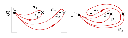
Figure 7: Braiding of two generic multi-contours.

This procedure was described in section 3.3 as an induction process to deform contours around $z_{2}$ in Figure 7 to pass to linear combinations of the types of loops illustrated in Figure 8 and then deform the resulting auxiliary loops into a set of basis contours like those in Figure 1.

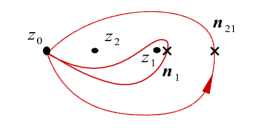
Figure 8: A set of auxiliary contours for the braiding calculation.

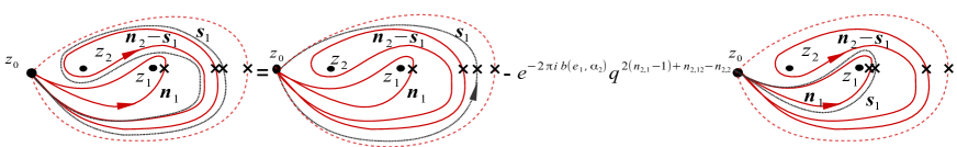
Figure 9: Deformation of the outermost of the contours encircling $z_{2}$.

Part 1:

The first part of the braiding calculation specifically deforms the contours around $z_{2}$ from Figure 7 to linear combinations of loops like in Figure 8. An intermediate step of this procedure is depicted in Figure 9. The ordered marked points $\mathsf{x}$ represent normalization points for the integral over the indicated contours, where the integrand is real. The gray contour being deformed in Figure 9 is associated with a $Q_{1}$ screening charge and carries the label $\mathbf{s}_{1}$. On the right hand side, this loop turns into a sum of two types of contours. The first is a loop around both points $z$ and has normalization point $\mathsf{x}$ at the same position as on the original contour. The second type however, is a loop around only the point $z_{1}$, whose normalization point is related by analytic continuation to the marked point $\mathsf{x}$ on the original gray contour. This means that the relative order of the marked points $\mathsf{x}$ has changed and as a consequence of the exchange relation (2.27), a braiding factor gets generated.

This factor contains a full monodromy $\text{e}^{-2\pi\text{i}b(e_{1},\alpha_{2})}$ due to moving the insertion point of the screening current $S_{1}$ counter-clockwise around $z_{2}$. The factor ${q}^{2(n_{2,1}-1)+n_{2,12}-n_{2,2}}$ then arises because one needs to relate the respective integrands defined by using two different choices of normalization points with the help of the exchange relation (2.27).

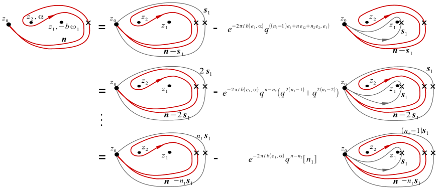
Figure 10: Example illustrating how quantum numbers arise in the braiding calculation.

Repeating the step described in Figure 9 generates quantum numbers $[n]=\frac{1-{q}^{2n}}{1-{q}^{2}}$, as illustrated in Figure 10, which has a generic vertex operator at $z_{2}$ and a degenerate operator at $z_{1}$. Let us explain a few more steps in this example, as it is relevant for one of the braiding calculations in which we are interested. We may denote $\gamma_{1}^{\mathbf{s}_{i}}$ the loop around $z_{1}$ which is associated with screening charges $Q_{1}$ and $Q_{12}$ for $i=1$ and $12$, respectively, and with no charge for $i=0$. If we then denote $\beta_{2}^{\mathbf{n}}$ the deformed loop around $z_{2}$ and $\beta_{21}^{\mathbf{n}_{21}}$ the loop around both points $z$ and denote $I[\beta_{21}^{\mathbf{n}_{21}}\beta^{\mathbf{n}}\gamma_{1}^{\mathbf{s}_{i}}]$ the integral over the indicated contours, then the intermediate results after resolving the contours associated with each type of screening charge are

$$I[\beta_{2}^{\mathbf{{n}}}\gamma_{1}^{\mathbf{s}_{0}}] =I[\beta_{21}^{n_{1}\mathbf{s}_{1}}\beta_{2}^{\mathbf{n}-n_{1}\mathbf{s}_{1}}\gamma_{1}^{\mathbf{s}_{0}}]-\text{e}^{-2\pi\text{i}b(e_{1},\alpha)}{q}^{n-n_{2}}[n_{1}]I[\beta_{21}^{(n_{1}-1)\mathbf{s}_{1}}\beta_{2}^{\mathbf{n}-n_{1}\mathbf{s}_{1}}\gamma_{1}^{\mathbf{s}_{1}}]$$ (C.1)

$$=I[\beta_{21}^{\mathbf{n}-n_{2}\mathbf{s}_{2}}\beta_{2}^{n_{2}\mathbf{s}_{2}}\gamma_{1}^{\mathbf{s}_{0}}]-\text{e}^{-2\pi\text{i}b(e_{12},\alpha)}{q}^{-2+n_{2}}[n]I[\beta_{21}^{n_{1}\mathbf{s}_{1}+(n-1)\mathbf{s}_{12}}\beta_{2}^{n_{2}\mathbf{s}_{2}}\gamma_{1}^{\mathbf{s}_{12}}]-$$

$$\quad~{}~{}-\text{e}^{-2\pi\text{i}b(e_{1},\alpha)}({q}^{-1}-{q}){q}^{-n_{2}}[n]I[\beta_{21}^{n_{1}\mathbf{s}_{1}+(n-1)\mathbf{s}_{12}+\mathbf{s}_{2}}\beta_{2}^{n_{2}\mathbf{s}_{2}}\gamma_{1}^{\mathbf{s}_{1}}]-$$

$$\quad~{}~{}-\text{e}^{-2\pi\text{i}b(e_{1},\alpha)}{q}^{n-n_{2}}[n_{1}]I[\beta_{21}^{(n_{1}-1)\mathbf{s}_{1}+n\mathbf{s}_{12}}\beta_{2}^{n_{2}\mathbf{s}_{2}}\gamma_{1}^{\mathbf{s}_{1}}]$$

$$=I[\beta_{21}^{\mathbf{n}}\gamma_{1}^{\mathbf{s}_{0}}]-\text{e}^{-2\pi\text{i}b(e_{1},\alpha)}({q}^{-1}-{q}){q}^{-n_{2}}[n]I[\beta_{21}^{\mathbf{n}-\mathbf{s}_{12}+\mathbf{s}_{2}}\gamma_{1}^{\mathbf{s}_{1}}]-$$

$$\quad~{}~{}-\text{e}^{-2\pi\text{i}b(e_{12},\alpha)}[n]\left({q}^{-2+n_{2}}+({q}^{-1}-{q}){q}^{-1-n_{2}}[n_{2}]\right)I[\beta_{21}^{\mathbf{n}-\mathbf{s}_{12}}\gamma_{1}^{\mathbf{s}_{12}}]-$$

$$\quad~{}~{}-\text{e}^{-2\pi\text{i}b(e_{1},\alpha)}{q}^{n-n_{2}}[n_{1}]I[\beta_{21}^{\mathbf{n}-\mathbf{s}_{1}}\gamma_{1}^{\mathbf{s}_{1}}]-\text{e}^{-2\pi\text{i}b(e_{12},\alpha){q}^{n-1-n_{2}}}[n_{1}][n_{2}]I[\beta_{21}^{\mathbf{n}-\mathbf{s}_{3}}\gamma_{1}^{\mathbf{s}_{12}}]~{}.$$

Note:

There are two additional technical observations to note here: i) contours associated with the composite screening charge $Q_{12}=Q_{1}Q_{2}-{q}Q_{2}Q_{1}$ are most safely treated when considered as linear combinations of contours for simple charges and ii) one must take care of the ordering of the newly generated contours, in particular when they are associated with the screening charges $Q_{12}$ and $Q_{2}$. Any reordering of contours implies a permutation of their associated normalization points, which generates braiding factors as illustrated for example by

$$\int_{\gamma}dyS_{1}(y)V_{\alpha}^{\mathbf{{n}}}(z)=V_{\alpha}^{\mathbf{{n}}+\mathbf{s}_{1}}(z)\qquad\mathrm{vs.}\qquad\int_{\gamma}dyS_{12}(y)V_{\alpha}^{\mathbf{{n}}}(z)={q}^{n_{1}}V_{\alpha}^{\mathbf{{n}}+\mathbf{s}_{12}}(z)~{}.$$ (C.2)

The case where a screening charge $Q_{2}$ is added has one additional feature. Changing the order of contours such that the $\mathbf{s}_{2}$ contour is inside of the loops with labels $\mathbf{s}_{1}$ means commuting an $S_{2}$ screening current past $S_{1}$, which by the definition of composite screening charges generates a current $S_{12}$ and thus

$$\int_{\gamma}dyS_{2}(y)V_{\alpha}^{\mathbf{{n}}}(z)={q}^{n_{12}-n_{1}}V_{\alpha}^{\mathbf{{n}}+\mathbf{s}_{2}}(z)-{q}^{-n_{1}}[n_{1}]V_{\alpha}^{\mathbf{{n}}+\mathbf{s}_{12}-\mathbf{s}_{1}}(z)~{}.$$ (C.3)

Part 2:

Resolving all of the deformed contours around the point $z_{2}$ in Figure 7, that are generated by the braiding procedure, creates a combination of the types of loops in Figure 8. The second part of the induction procedure described in section 3.3 is then the deformation of any such auxiliary loops that enclose both $z_{1}$ and $z_{2}$ in Figure 8 into combinations of the basis contours in Figure 1. An intermediate step is depicted in Figure 11. The same considerations as above apply here when deforming the gray contour on the left hand side. The resulting gray loops on the right have normalization points $\mathsf{x}$ that are either at the same position as on the original curve or moved to a different position and the integrands associated to different choices of normalization points are related by analytic continuation, which gives rise to a braiding factor. Furthermore, if the gray loop being deformed like in Figure 11 carries labels $\mathbf{s}_{12}$ or $\mathbf{s}_{2}$, it is necessary to reorder the resulting contours like we did in equations (C.2), (C.3) so that they match the order prescribed in Figure 1.

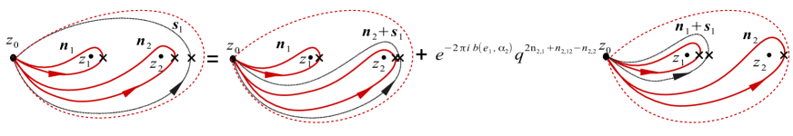
Figure 11: Decomposition of a simple contour associated with the root $e_{1}$ around two punctures into contours enclosing only one of the punctures.

Let us now take the contours in Figure 8 with a generic vertex operator inserted at the position $z_{2}$ and a degenerate operator at $z_{1}$ and deform the loop enclosing both points $z$ into a combination of basis contours like in Figure 1. This case is relevant to the braiding calculation of interest here. If we call $\gamma_{1}^{\mathbf{s}_{i}}$ the loop around $z_{1}$ and $\beta_{21}^{\mathbf{n}_{21}}$ the loop around both points $z$, then the decomposition of integrals over $\beta_{21}$-type contours leads to

$$I[\beta_{21}^{\mathbf{n}_{21}}\gamma_{1}^{\mathbf{s}_{0}}]={q}^{1-n}[n]I[\gamma_{2}^{\mathbf{n}_{21}-\mathbf{s}_{12}}\gamma_{1}^{\mathbf{s}_{12}}]+{q}^{1-n_{1}-n}[n_{1}]I[\gamma_{2}^{\mathbf{n}_{21}-\mathbf{s}_{1}}\gamma_{1}^{\mathbf{s}_{1}}]+{q}^{-n_{1}-n}I[\gamma_{2}^{\mathbf{n}_{21}}\gamma_{1}^{\mathbf{s}_{0}}],$$ (C.4)

$$I[\beta_{21}^{\mathbf{n}_{21}}\gamma_{1}^{\mathbf{s}_{1}}]={q}^{n_{1}-n_{2}}I[\gamma_{2}^{\mathbf{n}_{21}}\gamma_{1}^{\mathbf{s}_{1}}]-{q}^{n-n_{2}}[n_{2}]I[\gamma_{2}^{\mathbf{n}_{21}-\mathbf{s}_{2}}\gamma_{1}^{\mathbf{s}_{12}}]-{q}^{-1-n_{2}}(1-{q}^{2})[n]I[\gamma_{2}^{\mathbf{n}_{21}+\mathbf{s}_{1}-\mathbf{s}_{12}}\gamma_{1}^{\mathbf{s}_{12}}],$$

$$I[\beta_{21}^{\mathbf{n}_{21}}\gamma_{1}^{\mathbf{s}_{12}}]={q}^{n_{2}+n}I[\gamma_{2}^{\mathbf{n}_{21}}\gamma_{1}^{\mathbf{s}_{12}}],~{}~{}$$

with notation $I[\beta_{21}^{\mathbf{n}_{21}}\gamma_{1}^{\mathbf{s}_{i}}]$ for the integral over the indicated contours and where the loop $\gamma_{2}^{\mathbf{s}_{i}}$ is a basis contour enclosing the point $z_{2}$. Combining the two parts of the braiding calculation, we reach the main result.

Main result:

The two types of braid matrices that we compute following the steps outlined above have a degenerate vertex operator inserted at either the point $z_{1}$ or $z_{2}$ and are explicitly

$$\mathsf{B}[W_{\alpha,-b\omega_{1}}^{\ss_{k}-\delta_{\imath},\mathbf{{d}}_{\imath}}(z_{2},z_{1})] = \sum_{\jmath=1}^{3}(\mathsf{b}_{+})_{\imath\jmath}W_{-b\omega_{1},\alpha}^{\mathbf{{d}}_{\jmath},\ss_{k}-\delta_{\jmath}}(z_{1},z_{2})$$ (C.5)

$$\mathsf{B}[W_{-b\omega_{1},\alpha}^{\mathbf{{d}}_{\imath},\ss_{k}-\delta_{\imath}}(z_{2},z_{1})]=\sum_{\jmath=1}^{3}(\mathsf{b}_{-})_{\imath\jmath}W_{\alpha,-b\omega_{1}}^{\ss_{k}-\mathbf{{d}}_{\jmath},\mathbf{{d}}_{\jmath}}(z_{1},z_{2})~{}$$ (C.6)

using the notation $\ss_{k}=(s_{1}-k,k,s_{2}-k)$ and $\delta_{1}=(0,0,0),\delta_{2}=(1,0,0)$ and $\delta_{3}=(1,0,1)$. The matrix elements of $\mathsf{b}_{+}$ are

$$\mathsf{b}_{11}^{+} = {q}^{(h_{1},\nu)}~{},\qquad\mathsf{b}_{22}^{+}={q}^{(h_{2},\nu+e_{1})}~{},\qquad\mathsf{b}_{33}^{+}={q}^{(h_{3},\nu+e_{12})}$$ (C.7)

$$\mathsf{b}_{12}^{+} = {q}^{(h_{2},\nu+e_{1})}({q}-{q}^{-1}){q}^{-s_{2}-(e_{1},\lambda)}\left({q}^{1+2k}[s_{1}-k][1-s_{1}+s_{2}-k+(e_{1},\lambda)]+\mathsf{v}^{-1}[k]\right)$$

$$\mathsf{b}_{23}^{+} = {q}^{(h_{3},\nu+e_{12})}({q}^{-1}-{q})\left([s_{2}-k][1-s_{2}+k+(e_{2},\lambda)]{q}^{-(e_{2},\lambda)}-\mathsf{v}^{-1}[k]{q}^{1-2s_{2}+(e_{2},\lambda)}\right)$$

and

$$\mathsf{b}_{13}^{+}={q}^{(h_{3},\nu+e_{12})} (1-{q}^{2})\Big{(}[s_{1}-k][s_{2}-k][s_{2}-1-k-(e_{2},\lambda)]{q}^{1+4k-3s_{2}+(e_{2}-e_{1},\lambda)}$$ (C.8)

$$+\mathsf{v}^{-1}[k]\big{(}[s_{2}-2-(e_{12},\lambda)]{q}^{2-2k-s_{2}+(e_{12},\lambda)}-[s_{2}-k]{q}^{-2-s_{2}-(e_{12},\lambda)}$$

$$\qquad\qquad+[s_{1}-k]{q}^{2k-3s_{2}+(e_{2}-e_{1},\lambda)}+[s_{2}-k+1]{q}^{2k-2-3s_{2}+(e_{2}-e_{1},\lambda)}\big{)}$$

$$-{q}^{-1}\mathsf{v}^{-2}[k][k-1]{q}^{-3s_{2}-(e_{2}-e_{1},\lambda)}\Big{)}~{},$$

while those of $\mathsf{b}_{-}$ are

$$\mathsf{b}_{11}^{-} = {q}^{(h_{1},\nu)}~{},\qquad\mathsf{b}_{22}^{-}={q}^{(h_{2},\nu+e_{1})}~{},\qquad\mathsf{b}_{33}^{-}={q}^{(h_{3},\nu+e_{12})}$$ (C.9)

$$\mathsf{b}_{21}^{-} = {q}^{(h_{1},\nu)}({q}-{q}^{-1})~{},\qquad\mathsf{b}_{32}^{-}={q}^{(h_{2},\nu+e_{1})}({q}^{2}-1){q}^{-s_{1}+1}\left(\mathsf{v}{q}^{2k}[s_{1}-1-k]-{q}^{2k}\right)$$

$$\mathsf{b}_{31}^{-} = {q}^{(h_{1},\nu)}({q}-{q}^{-1})\mathsf{v}{q}^{s_{1}-1}~{}\qquad\qquad\qquad\qquad\qquad\qquad\qquad\qquad\qquad\qquad\qquad\qquad$$

for $\alpha=-b\lambda$ and $\nu=\lambda-s_{1}e_{1}-s_{2}e_{2}$.

Appendix D Realisation of the generators ${\mathsf{e}}_{i}$ on screened vertex operators

In this section we will indicate how to derive the identification between the action of $L_{-1}$ on screened vertex operators (3.30), which removes one contour of integration, and the action of ${\mathsf{e}}_{i}$ generators on tensor products of representations (3.31). Using notations similar to the ones introduced in section 3.4.1 for the simpler case of $\mathcal{U}_{q}({\mathfrak{s}}{\mathfrak{l}}_{2})$, we find that

$$\big{[}\,L_{-1}\,,\,{V}_{n}^{\alpha}(z)\,\big{]}-\partial_{z}{V}_{n}^{\alpha}(z)=S(z_{0})({q}-{q}^{-1}){\mathsf{k}}^{-1}{\mathsf{e}}{V}_{n-1}^{\alpha}(z),$$ (D.1)

by the following considerations. For screening number $n=2$, there are only two contours of integration. $L_{-1}$ acts by the Leibniz rule on each screening current in ${V}_{n}^{\alpha}(z)$, producing total derivative terms. The contributions from the two boundaries of the integration contour are related by monodromy factors. In this way it is not hard to arrive at the following equation

$$\big{[}\,L_{-1}\,,\,V_{2}^{\alpha}(z)\,\big{]}=\oint dy(1-\text{e}^{-4\pi\text{i}b(\alpha+b)})S(z_{0})S(y)+(1-\text{e}^{-4\pi\text{i}b\alpha})S(y)S(z_{0})V_{\alpha}(z)+\partial_{z}V_{2}^{\alpha}(z)~{}.$$

By factoring off the operator $S(z_{0})$, this simplifies to

$$\big{[}\,L_{-1}\,,\,V_{2}^{\alpha}(z)\,\big{]}={q}^{2(1-\lambda_{\alpha})}({q}-{q}^{-1})^{-1}({q}^{2\lambda_{\alpha}-1}-{q}^{-2\lambda_{\alpha}+1})({q}^{2}-{q}^{-2})S(z_{0})V_{1}^{\alpha}(z)+\partial_{z}V_{2}^{\alpha}(z)~{}.$$

More generally, for arbitrary $n\in\mathbb{N}$ units of screening charge, we find by iterating these steps

$$\big{[}\,L_{-1}\,,\,V^{n}_{\alpha}(z)\,\big{]}=\partial_{z}V_{n}^{\alpha}(z)+{q}^{2(n-1-\lambda)}({q}-{q}^{-1})^{-1}({q}^{2\lambda-n+1}-{q}^{-2\lambda+n-1})({q}^{n}-{q}^{-n})S(z_{0})V_{n-1}^{\alpha}(z)~{}.$$

To compare now with the actions of the ${\mathsf{e}}$ and ${\mathsf{k}}$ generators, notice that these are

$${\mathsf{e}}~{}e^{\lambda}_{n}=({q}-{q}^{-1})^{-2}({q}^{2\lambda-n+1}-{q}^{-2\lambda+n-1})({q}^{n}-{q}^{-n})e^{\lambda}_{n-1}~{},\quad{\mathsf{k}}^{-1}~{}e^{\lambda}_{n-1}={q}^{2(n-1-\lambda)}e^{\lambda}_{n-1}~{},$$

so we arrive indeed at equation (D.1).

At higher rank, for $\mathcal{U}_{q}({\mathfrak{s}}{\mathfrak{l}}_{3})$, one can similarly show for example

$$\big{[}\,L_{-1}\,,\,{V}_{\mathbf{n}}^{\alpha}(z)\,\big{]}-\partial_{z}{V}_{\mathbf{n}}^{\alpha}(z)\sim({q}-{q}^{-1})\left({\mathsf{k}}_{1}^{-1}{\mathsf{e}}_{1}+{\mathsf{k}}_{2}^{-1}{\mathsf{e}}_{2}\right){V}_{\mathbf{n}}^{\alpha}(z)$$ (D.2)

The final observation to make in order to identify the actions of $L_{-1}$ and ${\mathsf{e}}$ is that the action of $L_{-1}$ on composite screened vertex operators correctly reproduces the action of the coproduct

$$\big{[}\,L_{-1}\,,\,{V}_{\mathbf{{n}}_{m},\ldots,\mathbf{{n}}_{1}}^{\alpha_{m},\ldots,\alpha_{1}}(z_{m},\ldots,z_{1})\,\big{]}-\sum_{l=1}^{m}\partial_{z_{l}}{V}_{\mathbf{{n}}_{m},\ldots,\mathbf{{n}}_{1}}^{\alpha_{m},\ldots,\alpha_{1}}(z_{m},\ldots,z_{1})\sim(\Delta(x){V}_{\mathbf{{n}}_{m},\ldots,\mathbf{{n}}_{1}}^{\alpha_{m},\ldots,\alpha_{1}})(z_{m},\ldots,z_{1}),$$

for

$$x=(q-q^{-1})({\mathsf{k}}_{1}^{-1}{\mathsf{e}}_{1}+{\mathsf{k}}_{2}^{-1}{\mathsf{e}}_{2}),$$

which we verified by direct computation.

In order to see that the boundary terms occurring in the commutators with arbitrary generators of the $W$-algebra admit a similar representation in terms of the generators ${\mathsf{e}}_{i}$ the main point to observe is that all commutators between screening currents and $W$-generators can be represented as total derivatives.

References

• [AGT] L.ย F.ย Alday, D.ย Gaiotto, and Y.ย Tachikawa, Liouville Correlation Functions from Four-dimensional Gauge Theories, Lett. Math. Phys. 91 (2010) 167โ€“197.
• [AGGTV] L. F. Alday, D. Gaiotto, S. Gukov, Y. Tachikawa, H. Verlinde, Loop and surface operators in $\mathcal{N}=2$ gauge theory and Liouville modular geometry, J. High Energy Phys. 1001 (2010) 113.
• [BMPTY] L. Bao, V. Mitev, E. Pomoni, M. Taki, F. Yagi, Non-Lagrangian Theories from Brane Junctions, JHEP 1401 (2014) 175.
• [BFS] R. Bezrukavnikov, M. Finkelberg, V. Schechtman, Factorisable sheaves and quantum groups, Lecture Notes in Mathematics 1691, Springer Verlag, Berlin, 1998.
• [BMP] P. Bouwknegt, J. McCarthy, K. Pilch, Free field approach to two-dimensional conformal field theories, Prog. Theor. Phys. Suppl. 102 (1990) 67-135.
• [Bu] M. Bullimore, Defect Networks and Supersymmetric Loop Operators, JHEP 1502 (2015) 066.
• [BT1] A.ย G.ย Bytsko and J.ย Teschner, $R$-operator, co-product and Haar-measure for the modular double of $U_{q}({\mathfrak{s}}{\mathfrak{l}}(2,\mathbb{R}))$. Comm. Math. Phys. 240 (2003) 171โ€“196.
• [CF] L.O. Chekhov, V. Fock: A quantum Teichmรผller space, Theor. Math. Phys. 120 (1999) 1245โ€“1259
• [CGT] I. Coman, M. Gabella, J. Teschner, Line operators in theories of class $\mathcal{S}$, quantized moduli space of flat connections, and Toda field theory, JHEP 1510 (2015) 143.
• [DGOT] N. Drukker, J. Gomis, T. Okuda, J. Teschner, Gauge Theory Loop Operators and Liouville Theory, J. High Energy Phys. 1002 (2010) 057.
• [F95] L. D.ย Faddeev, Discrete Heisenberg-Weyl Group and Modular Group, Lett. Math. Phys. 34 (1995) 249-254.
• [F99] L. D.ย Faddeev, Modular double of a quantum group, Conf rence Mosh Flato 1999, Vol. I (Dijon), 149โ€“156, Math. Phys. Stud., 21, Kluwer Acad. Publ., Dordrecht, 2000, arXiv:math/9912078.
• [FL] V. A. Fateev, A. V. Litvinov, Correlation functions in conformal Toda field theory I, JHEP 0711 (2007) 002.
• [FW] G. Felder, C. Wiecerkowski, Topological representations of the quantum group $U_{q}({\mathfrak{s}}{\mathfrak{l}}(2))$, Comm. Math. Phys. 138 (1991) 583-605.
• [FG1] V.V. Fock, A. Goncharov, Moduli spaces of local systems and higher Teichmรผller theory. Publ. Math. Inst. Hautes ร‰tudes Sci. 103 (2006) 1โ€“211.
• [FG2] Fock, V. V.; Goncharov, A. B. The quantum dilogarithm and representations of quantum cluster varieties. Invent. Math. 175 (2009) 223โ€“286.
• [FI] I. Frenkel, I. Ip, Positive representation of split real quantum groups and future perspectives, International Mathematics Research Notices, 2014 (8) (2014) 2126-2164
• [Ga] D. Gaiotto, N=2 dualities, JHEP 1208 (2012) 034.
• [GMN] D. Gaiotto, G. Moore and A. Neitzke, Wall-crossing, Hitchin systems, and the WKB approximation. Adv. Math. 234 (2013) 239โ€“403.
• [Go] W. Goldman, Convex real projective structures on compact surfaces, J. Differential Geom. 31 (1990) 126-159.
• [GS] C. Gomez, G. Sierra, The Quantum Symmetry of Rational Conformal Field Theories, Nucl.Phys. B352 (1991) 791-828 .
• [GLF1] J. Gomis, B. Le Floch, โ€™t Hooft Operators in Gauge Theory from Toda CFT, JHEP 1111 (2011) 114.
• [GLF2] J. Gomis, B. Le Floch, M2-brane surface operators and gauge theory dualities in Toda, JHEP 1604 (2016) 183.
• [GOP] J. Gomis, T. Okuda and V. Pestun, Exact results for โ€™t Hooft loops in gauge theories on $S^{4}$, JHEP 1205 (2012) 141.
• [Hi] N. Hitchin, Lie group and Teichmรผller space, Topology 31 (1992) 449โ€“473.
• [HK] L. Hollands, O. Kidwai, Higher length-twist coordinates, generalized Heunโ€™s opers, and twisted superpotentials, Preprint arXiv:1710.04438.
• [HN] L. Hollands, A. Neitzke, Spectral Networks and Fenchelโ€“Nielsen Coordinates, Lett. Math. Phys. 106 (2016) 811โ€“877.
• [ILT] N. Iorgov, O. Lisovyy, J. Teschner, Isomonodromic tau-functions from Liouville conformal blocks, Comm. Math. Phys. 336 (2015) 671-694.
• [IMP] M. Isachenkov, V. Mitev, E. Pomoni, Toda 3-Point Functions From Topological Strings II, JHEP 1608 (2016) 066.
• [IOT] Y. Ito, T. Okuda and M. Taki, Line operators on $S^{1}\times R^{3}$ and quantization of the Hitchin moduli space, JHEP 1204 (2012) 010.
• [Ji] M. Jimbo, Monodromy problem and the boundary condition for some Painlev equations. Publ. Res. Inst. Math. Sci. 18 (1982) 1137?1161 (1982)
• [Ka1] R.M. Kashaev: Quantization of Teichmรผller spaces and the quantum dilogarithm, Lett. Math. Phys. 43 (1998) 105-115.
• [Ka2] R. M. Kashaev, The quantum dilogarithm and Dehn twists in quantum Teichmรผller theory. Integrable structures of exactly solvable two-dimensional models of quantum field theory (Kiev, 2000), 211โ€“221, NATO Sci. Ser. II Math. Phys. Chem., 35, Kluwer Acad. Publ., Dordrecht, 2001.
• [Ki] H.C. Kim, The symplectic global coordinates on the moduli space of real projective structures, J. Differential Geom. 53 (1999) 359-401.
• [La1] S. Lawton, Generators, Relations and Symmetries in Pairs of 3x3 Unimodular Matrices, J. Algebra 313 (2007), no. 2, 782โ€“801, Preprint math/0601132.
• [La2] S. Lawton, Poisson Geometry of $SL(3,C)$-Character Varieties Relative to a Surface with Boundary, Trans. Amer. Math. Soc. 361 (2009) 2397โ€“2429, Preprint math/0703251.
• [LF] B. Le Floch, S-duality wall of SQCD from Toda braiding, Preprint arXiv:1512.09128.
• [MP] V. Mitev, E. Pomoni, Toda 3-Point Functions From Topological Strings JHEP 1506 (2015) 049.
• [NRS] N. Nekrasov, A. Rosly, S. Shatashvili, Darboux coordinates, Yang-Yang functional, and gauge theory, Nucl. Phys. Proc. Suppl.ย 216 (2011) 69โ€“93.
• [NS] N. Nekrasov, S. Shatashvili, Quantization of Integrable Systems and Four Dimensional Gauge Theories, Proceedings of the 16th International Congress on Mathematical Physics, Prague, August 2009, P. Exner, Editor, pp.265-289, World Scientific 2010.
• [NT] I. Nidaiev, T. Teschner, On the relation between the modular double of $U_{q}({\mathfrak{s}}{\mathfrak{l}}(2,R))$ and the quantum Teichmueller theory, Preprint arXiv:1302.3454.
• [Pe] R.C. Penner, The decorated Teichmรผller space of punctured surfaces, Comm. Math. Phys. 113 (1987) 299โ€“339.
• [PT1] B.ย Ponsot and J.ย Teschner, Liouville bootstrap via harmonic analysis on a noncompact quantum group, arXiv:hep-th/9911110.
• [PT2] B.ย Ponsot and J.ย Teschner, Clebsch-Gordan and Racah-Wigner coefficients for a continuous series of representations of $U_{q}({\mathfrak{s}}{\mathfrak{l}}(2,\mathbb{R}))$, Commun.ย Math.ย Phys.ย  224 (2001) 613โ€“655.
• [RRR] C. Ramirez, H. Ruegg, M. Ruiz-Altaba, The Contour picture of quantum groups: Conformal field theories. Nucl.Phys. B364 (1991) 195-233.
• [SS1] G. Schrader, A. Shapiro, A cluster realization of $U_{q}(\mathfrak{sl}_{n})$ from quantum character varieties, Preprint arXiv:1607.00271.
• [SS2] G. Schrader, A. Shapiro, Continuous tensor categories from quantum groups I: algebraic aspects, Preprint arXiv:1708.08107.
• [T01] J.ย Teschner, Liouville theory revisited, Class.ย Quant.ย Grav.ย  18 (2001) R153โ€“R222.
• [T03] J. Teschner, On the relation between quantum Liouville theory and the quantized Teichmรผller spaces, Int. J. Mod. Phys. A19S2 (2004) 459โ€“477.
• [T10] J. Teschner, Quantization of the Hitchin moduli spaces, Liouville theory, and the geometric Langlands correspondence I. Adv. Theor. Math. Phys. 15 (2011) 471โ€“564.
• [T17] J. Teschner A guide to two-dimensional conformal field theory, to appear in the proceedings of the Les Houches Summer School, Session 106: Integrability: from Statistical Systems to Gauge Theory, Les Houches, France, June 6โ€“July 1, 2016, Preprint arXiv:1708.00680.
• [TV] J. Teschner, G. S. Vartanov, Supersymmetric gauge theories, quantization of moduli spaces of flat connections, and conformal field theory. Adv. Theor. Math. Phys. 19 (2015) 1โ€“135.
• [TW] Y. Tachikawa, Watanabe, On skein relations in class S theories, JHEP 1506 (2015) 186.
• [ZZ] A.B. and Al.B. Zamolodchikov, Structure constants and conformal bootstrap in Liouville field theory, Nucl. Phys. B477 (1996), 577โ€“605.