On quality of implementation of Fortran 2008 complex intrinsic functions on branch cuts

Abstract

Branch cuts in complex functions in combination with signed zero and signed infinity have important uses in fracture mechanics, jet flow and aerofoil analysis. We present benchmarks for validating Fortran 2008 complex functions - LOG, SQRT, ASIN, ACOS, ATAN, ASINH, ACOSH and ATANH - on branch cuts with arguments of all 3 IEEE floating point binary formats: binary32, binary64 and binary128. Results are reported with 8 Fortran 2008 compilers: GCC, Flang, Cray, Oracle, PGI, Intel, NAG and IBM. Multiple test failures were revealed, e.g. wrong signs of results or unexpected overflow, underflow, or NaN. We conclude that the quality of implementation of these Fortran 2008 intrinsics in many compilers is not yet sufficient to remove the need for special code for branch cuts. The test results are complemented by conformal maps of the branch cuts and detailed derivations of the values of these functions on branch cuts, to be used as a reference. The benchmarks are freely available from cmplx.sf.net. This work will be of interest to engineers who use complex functions, as well as to compiler and maths library developers.

1 Introduction

In the following $w=u+\textrm{i}v$ and $z=x+\textrm{i}y$ are complex variables, and $w=w(z)$ is a conformal mapping function from $z$ to $w$. $\Re z$ and $\Im z$ are the real and the imaginary parts of $z$. Fortran functions and named constants are written in monospaced font.

Fortran intrinsic functions SQRT and LOG accepted complex arguments at least since FORTRAN66 standard [1]. IEEE floating point standard [2] defined signed zero and signed infinity: $+0,-0,+\infty,-\infty$. Fortran 95 standard [3] added support for IEEE floating point arithmetic. Fortran 2008 standard [4] added support for complex arguments to intrinsic functions ACOS, ASIN, ATAN and 3 new inverse hyperbolic intrinsics: ACOSH, ASINH, ATANH, all of which also accept complex arguments.

These 8 complex elementary functions, together with IEEE style signed zero and infinity, have useful applications e.g. in fracture mechanics, because a branch cut can represent a mathematical crack. Perhaps the oldest and simplest example is function

$$z=w+\frac{1}{w}$$ (1)

which maps a complex plane with a cut unit circle onto a complex plane with a cut along $x$ at $-2\leq x\leq 2$. This function has been in use probably since early 20th century, see e.g. [5, 6]. It is still widely used in fracture mechanics today [7]. In practice the inverse of Eqn. (1) is more useful:

$$w=\frac{1}{2}(z+\textrm{copySign}(1,\Re z)\sqrt{z^{2}-4})$$ (2)

where copySign is an IEEE function which returns a value with the magnitude of the first argument and the sign of the second argument [8]. The map of Eqn. (2) is shown in Fig. 1

Figure 1: Map of $w=\frac{1}{2}(z+\textrm{copySign}(1,\Re z)\sqrt{z^{2}-4})$. The branch cut ABCD in $z$ is mapped onto a unit circle ABCD in $w$.

Note that Eqn. (2) produces the desired mapping only if $+0$ and $-0$ can be distinguished, so that points in $z$ on the top and the bottom boundary of the cut, i.e. with $y=+0$ and $y=-0$ are mapped respectively onto the top and the bottom boundary of the unit circle in $w$. For example point $z=0-\textrm{i}0$ is mapped to point $w=0-\textrm{i}1$, point B in Fig. 1, and point $z=0+\textrm{i}0$ is mapped to point $w=0+\textrm{i}1$, point D in Fig. 1.

$\log z$ has a single branch cut along the negative real axis, therefore it can be used for analysis of an edge crack in an infinite plate. A map of $w=\log z$ is shown in Fig. 2.

Figure 2: Map of the branch cut of $w=\log z$. Points A, B, C are on the top boundary of the cut, $y=+0$. Points D, E, F are on the bottom boundary of the cut, $y=-0$.

The 3 inverse trigonometric ($\arcsin$ , $\arccos$ and $\arctan$) and the 2 inverse hyperbolic functions ($\operatorname{arcsinh}$ and $\operatorname{arctanh}$) have 2 cuts on either the real or the imaginary axis, and can therefore be used for the analysis of bodies with 2 cracks along the same line, e.g. an infinite or a finite width plate with 2 opposing cracks with a finite ligament length in between. This case is of significant practical importance in fracture mechanics, see e.g. [9, Sec. 4, ‘Parallel Cracks’].

The third inverse hyperbolic function, $\operatorname{arccosh}$, has a single branch cut and can be used for an edge crack geometry.

Another interesting case is function $w=\tan(\arccos z^{2}/4)$ [5, p. 79] which maps a plane with 2 intersecting cuts onto an upper half plane, $v\geq 0$. The two cuts form a cross centred at the origin, see Fig. 3.

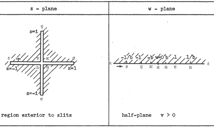
Figure 3: Map of function $w=\tan(\arccos z^{2}/4)$, reproduced from [5].

Jet flows and aerofoils are among other popular practical examples where signed zero is required to obtain correct conformal maps of multivalued complex functions on branch cuts [10, 11].

The usage of $-0$ was further popularised, although with no new examples, in [12, 13].

Although algorithms can be, and have been, developed which use data a short distance away from the cuts, this is not very satisfactory, as it is not an obvious question what this small distance should be. In addition, branch cuts often contain the most important data, e.g. the extremum values of crack tip displacement fields are found on crack flanks, which is useful in experimental fracture mechanics analysis [14]. It would help algorithm developers and programmers significantly if they had full confidence that intrinsics behave correctly on branch cuts, and no special cases need to be considered and coded for.

Expressions for these 8 complex intrinsic, which deal correctly with $\pm 0,\pm\infty$ and NaN, and avoid cancellation, were given by W. Kahan in 1987 [10]. A recent study concludes that no better expressions have been proposed since then [15].

Accuracy of complex floating point calculations was analysed in a number of works. Expressions for the relative errors of complex $\sqrt{}$ and $\log$ (as well as $\exp$, $\sin$, $\cos$) are given in [16], although the authors did not distinguish $+0$ and $-0$. The expressions are given in terms of the relative errors of the real counterparts of these intrinsics, e.g. their bound for the relative error in complex $\sqrt{}$ is $2\epsilon+1.5E_{\textrm{sqrt}}$, where $E_{\textrm{sqrt}}$ is the relative error bound for real $\sqrt{}$. [17] proposed a high speed implementation of complex $\sqrt{}$ which preserved the accuracy of [16]. For complex $\log$ [16] gives the relative error bound of $3.886\epsilon+E_{\log}$, where $E_{\log}$ is the relative error bound for real $\log x,x\gg 1$. For $\arcsin$ and $\arccos$ [18] give the relative error bound of $9.5\epsilon$. The relative error bound of a fused multiply-add (FMA) for complex multiplication was recently estimated as low as $\epsilon$ [19].

This brief introduction shows the practical importance, in fracture mechanics and other areas of engineering, of such seemingly esoteric tools as signed zero and signed infinity. On the other hand, Fortran is still the most widely used language for scientific and engineering computations, particularly in high performance computing (HPC), where Fortran codes use 60-70% of machine cycles [20]. Therefore the question of how well the above 8 complex functions are implemented in modern Fortran deserves attention. This question is addressed in this work with the introduction of a set of benchmarks with 70 tests, which check correctness of the 8 intrinsics on branch cuts. The code used in this work is freely available from cmplx.sf.net.

2 Tests

The tests are designed to verify the behaviour of the 8 intrinsic Fortran functions at special points on branch cuts. The reference expressions used for validating the results from the test programs are derived in the Appendix. All three IEEE basic binary formats are verified: binary32, binary64 and binary128 [8].

To aid portability, Fortran 2008 intrinsic module iso_fortran_env includes named constants for these IEEE data formats: REAL32, REAL64 and REAL128, which are used to define the kinds of real and complex variables and constants in the tests as e.g:

⬇

use, intrinsic :: iso_fortran_env

integer, parameter :: fk=real64

real(kind=fk), parameter :: one=1.0_fk

The tests check that signs of the real and the imaginary parts are correct, and that no undue overflow, underflow or NaN results are produced. Fortran IEEE intrinsics IEEE_CLASS, IEEE_COPY_SIGN, IEEE_IS_FINITE, IEEE_IS_NAN, IEEE_SUPPORT_SUBNORMAL, IEEE_SUPPORT_INF, IEEE_SUPPORT_NAN, IEEE_VALUE are used, as well as named constants ieee_negative_inf, ieee_positive_inf, ieee_negative_zero and ieee_positive_zero. For example, the values of $\pm 0$ and $\pm\infty$ are defined in the tests as:

⬇

real(kind=fk) :: infp, infm, zerop, zerom

infp=ieee_value( one, ieee_positive_inf )

infm=ieee_value( one, ieee_negative_inf )

zerop=ieee_value( one, ieee_positive_zero )

zerom=ieee_value( one, ieee_negative_zero )

In addition, Fortran intrinsics HUGE, TINY and EPSILON are used, which return the largest and the smallest positive model numbers respectively, denoted $h$ and $t$, and machine epsilon, $\epsilon$. Note that the Fortran definition of $\epsilon$ is $\epsilon=r^{1-p}$, where $r$ is the radix, $r=2$ on binary computers, and $p$ is the precision. This definition follows the IEEE standard [8].

To help the reader understand the tests, the maps of the branch cuts for each of the 8 functions are given in the following sections. The values of $z$ and $w$ at all tested special points are given on each map. The plots were calculated using REAL64 real and complex kind with gfortran8 compiler.

2.1 LOG

Behaviour of LOG was checked on the branch cut at 6 points: $z=-h\pm\textrm{i}0$, $z=-1\pm\textrm{i}0$ and $z=-t\pm\textrm{i}0$. The top and the bottom boundaries of the cut are mapped to $w=u+\textrm{i}\pi$ and $w=u-\textrm{i}\pi$ respectively, see Fig. 2.

2.2 SQRT

Behaviour of SQRT was checked on the branch cut at 8 points: $z=-h\pm\textrm{i}0$, $z=-1\pm\textrm{i}0$, $z=-t\pm\textrm{i}0$ and $z=0\pm\textrm{i}0$. The top boundary of the cut is mapped onto the positive imaginary axis, and the bottom boundary of the cut is mapped onto the negative imaginary axis, see Fig. 4.

Figure 4: Map of the branch cut of $w=\sqrt{z}$. Points A and B are on the top boundary of the cut, $y=+0$. Points C and D are on the bottom boundary of the cut, $y=-0$.

2.3 ASIN

$w=\arcsin z$ maps a plane with 2 cuts along the real axis, $x\leq-1$ and $x\geq 1$ to an infinite strip of width $\pi$ along the imaginary axis, $-\pi/2\leq u\leq\pi/2$. The left cut, $x\leq-1$ is mapped onto the left boundary of the strip, $u=-\pi/2$. The right cut, $x\geq 1$ is mapped onto the right boundary of the strip, $u=\pi/2$, as shown in Fig. 5. Behaviour of ASIN was checked on 8 points: $z=\pm h\pm\textrm{i}0$ and $z=\pm 1\pm\textrm{i}0$.

Figure 5: Map of $w=\arcsin z$. Points A, B, E, F are on the top boundary of the cut, $y=+0$. Points C, D, G, H are on the bottom boundary of the cut, $y=-0$. Points B and C are at $x=-1$. Points F and G are at $x=1$.

2.4 ACOS

$w=\arccos z$ has 2 branch cuts, both on the real axis, at $x\leq-1$ and $x\geq 1$, see Fig. 6. For $x\leq-1$, the top boundary of the cut, $y=+0$, is mapped to $w=\pi-\textrm{i}b$ and the bottom boundary of the cut, $y=-0$, is mapped to $w=\pi+\textrm{i}b$. For $x\geq 1$, the top boundary of the cut, $y=+0$, is mapped to $w=0-\textrm{i}b$, and the bottom boundary of the cut, $y=-0$, is mapped to $w=0+\textrm{i}b$. In all cases $b\geq 0$. Behaviour of ACOS was checked on the same 8 points as of ASIN.

Figure 6: Map of the branch cut of $w=\arccos z$. In plane $z$ points A, B, E, F are on the top boundary of the cut, $y=+0$. Points C, D, G, H are on the bottom boundary of the cut, $y=-0$. Points B and C are at $x=-1$. Points F and G are at $x=1$.

2.5 ATAN

$w=\arctan z$ maps a plane with 2 cuts along the imaginary axis, $y\leq-1$ and $y\geq 1$ to an infinite strip along the imaginary axis of width $\pi$ and centred on zero, see Fig. 7.

Behaviour of ATAN was checked in 12 points: $z=\pm 0\pm\textrm{i}h$, $z=\pm 0\pm\textrm{i}1$ and $z=\pm 0\pm\textrm{i}(1+\epsilon)$. The last 4 values are interesting because they are likely to be used as the best substitute for $\pm 0\pm\textrm{i}1$ on systems which do not support $\pm\infty$.

Note that in Fig. 7, $|\Im(\arctan(\pm 0\pm\textrm{i}1))|\approx 5.6\times 10^{-309}$ is subnormal, the smallest REAL64 normal number being $\approx 2.2\times 10^{-308}$. Note that [8] uses the term subnormal instead of the earlier denormal. On systems with no support for subnormals the correct result is $\Im(\arctan(\pm 0\pm\textrm{i}1))=\pm 0$, with the correct sign. On the other hand, on systems with no support for subnormals, a subnormal return value is not acceptable, because such value, $k$, would violate the expected inequalities $|k|>0$ and $|k|<t$, [4].

Also note that the exact value of $\Re(\arctan(\pm 0\pm\textrm{i}1))$ is immaterial, provided it’s finite. For consistency with the other values of $\arctan$ on the cuts, and for aesthetic pleasure, $\pm\pi/2$ might be preferred, but the actual value has no influence on consecutive operations made with the result of $\arctan(\pm 0\pm\textrm{i}1)$, because these will be determined solely by the infinite imaginary part.

Figure 7: Map of the branch cut of $w=\arctan z$. Points A, B, E, F are at $x=+0$. Points C, D, G, H are at $x=-0$.

2.6 ASINH

$w=\operatorname{arcsinh}z$ maps a plane with 2 cuts along the imaginary axis, $y\leq-1$ and $y\geq 1$ to an infinite strip of width $\pi$ along the real axis, $-\pi/2\leq v\leq\pi/2$. The bottom cut, $y\leq-1$ is mapped onto the bottom boundary of the strip, $v=-\pi/2$. The top cut, $y\geq 1$ is mapped onto the top boundary of the strip, $v=\pi/2$, as shown in Fig. 8. Behaviour of ASINH is checked on 8 points: $z=\pm 0\pm\textrm{i}h$ and $z=\pm 0\pm\textrm{i}1$.

Figure 8: Map of $w=\operatorname{arcsinh}z$. Points A, B, E, F are at $x=+0$. Points C, D, G, H are at $x=-0$. Points B, C are at $y=1$. Points F, G are at $y=-1$.

2.7 ACOSH

$w=\operatorname{arccosh}z$ maps a plane with a single cut along the real axis at $x\leq 1$ onto a semi-infinite strip of width $2\pi$, running along the real axis, $u\geq 0$, see Fig. 9.

Figure 9: Map of $w=\operatorname{arccosh}z$. Points A, B, E, F are at $x=+0$. Points C, D, G, H are at $x=-0$. Points B, C are at $y=1$. Points F, G are at $y=-1$.

The tests check that (1) the top side of the cut at $x\leq-1$ is mapped onto the top boundary of the strip, $u\geq 0,v=\pi$; (2) the top side of the cut at $-1\leq x\leq 1$ is mapped onto the end of the strip at $u=0,0\leq v\leq\pi$; (3) the bottom side of the cut at $-1\leq x\leq 1$ is mapped onto the end of the strip at $u=0,-\pi\leq v\leq 0$, and (4) the bottom side of the cut at $x\leq-1$ is mapped onto the bottom boundary of the strip, $u\geq 0,v=-\pi$. Thus, behaviour of ACOSH is checked on 8 points: $z=-h\pm\textrm{i}0$, $z=-1\pm\textrm{i}0$, $z=0\pm\textrm{i}0$ and $z=1\pm\textrm{i}0$.

2.8 ATANH

$w=\operatorname{arctanh}z$ maps a plane with 2 cuts along the real axis, $x\leq-1$ and $x\geq 1$ onto a infinite strip of width $\pi$ centered on 0 and running along the real axis, see Fig. 10. ATANH was verified on 12 points: $z=\pm h\pm\textrm{i}0$, $z=\pm 1\pm\textrm{i}0$ and $z=\pm(1+\epsilon)\pm\textrm{i}0$. Behaviour of ATANH on the branch cuts mirrors many features of that of ATAN, see Sec. 2.5.

Figure 10: Map of $w=\operatorname{arctanh}z$. Points A, B, E, F are at $x=+0$. Points C, D, G, H are at $x=-0$. Points B and C are at $y=1$. Points F and G are at $y=-1$.

3 Results

Fortran compilers, compiler options operating systems and CPUs used in this study are detailed in Tab. 1.

Compiler	Compiler options	OS	CPU
gfortran 8.0	-fsign-zero	FreeBSD	Haswell
Flang 4.0	-Kieee	FreeBSD	Haswell
Cray 8.5.8	-hfp0	linux	IvyBridge
Oracle 12.6 Fortran 95 8.8	-fsimple=0 -ftrap=none	linux	SandyBridge
PGI 16.3-0	-Kieee	linux	SandyBridge
Intel 18.0.1	-assume minus0	linux	Broadwell
NAG 6.2(Chiyoda) Build 6201	-ieee=full	linux	Broadwell
IBM XL Fortran 15.1.5	-qstrict	linux	Power8

Table 1: Compilers, compiler options, operating systems and CPUs used in this work.

Flang (github.com/flang-compiler) is an open source front end based on Nvidia PGI compiler, targeting LLVM. Flang 4.0 does not support inverse hyperbolic intrinsics.

Oracle 12.6 Fortran 95 compiler, released in May 2017, supports some Fortran 2003 and 2008 features, but not complex arguments for inverse trigonometric intrinsics.

PGI 16.3-0 does not support complex arguments to inverse hyperbolic intrinsics.

The results are presented in the form of tables. The dot entry, ”$\cdot$”, means the test has passed. Several kinds of test failures are distinguished, as detailed in Tab. 2.

Symbol	Failure type
$\times$	intrinsic not implemented with this argument
$d$	subnormal value returned, but subnormals are not supported
$m$	wrong magnitude of finite non-zero real/imaginary part
$n$	NaN, the correct value is finite or infinite
$o$	unwarranted overflow, the correct value is finite
$p$	normal finite non-zero result, the correct value is 0
$s$	wrong sign of real/imaginary part, or both
$z$	zero real/imaginary part, the correct value is normal finite non-zero

Table 2: List of test failure types. The symbols are used in Tabs. LABEL:tab:monkey, LABEL:tab:apple and LABEL:tab:pear.

Multiple failures are possible in a single test, e.g. an entry ”$osz$” means that failures of kind ”$o$”, ”$s$” and ”$z$” have occurred in that test. Most failure types are self-explanatory, except type ”$m$”, which is justified in App. A.9.

3.1 REAL32

For REAL32 real and complex variables $h\approx 3.4\times 10^{38}$, $t\approx 1.2\times 10^{-38}$ and $\epsilon\approx 1.2\times 10^{-7}$. The test results are summarised in Tab. LABEL:tab:monkey.

Test	GCC	Flang	Cray	Oracle	PGI	Intel	NAG	IBM
$\log(-h+\textrm{i}0)$	$\cdot$	$\cdot$	$\cdot$	$\cdot$	$\cdot$	$\cdot$	$\cdot$	$\cdot$
$\log(-1+\textrm{i}0)$	$\cdot$	$\cdot$	$\cdot$	$\cdot$	$\cdot$	$\cdot$	$\cdot$	$\cdot$
$\log(-t+\textrm{i}0)$	$\cdot$	$\cdot$	$\cdot$	$\cdot$	$\cdot$	$\cdot$	$\cdot$	$\cdot$
$\log(-t-\textrm{i}0)$	$\cdot$	$\cdot$	$\cdot$	$\cdot$	$\cdot$	$\cdot$	$\cdot$	$\cdot$
$\log(-1-\textrm{i}0)$	$\cdot$	$\cdot$	$\cdot$	$\cdot$	$\cdot$	$\cdot$	$\cdot$	$\cdot$
$\log(-h-\textrm{i}0)$	$\cdot$	$\cdot$	$\cdot$	$\cdot$	$\cdot$	$\cdot$	$\cdot$	$\cdot$
$\sqrt{-h+\textrm{i}0}$	$\cdot$	$o$	$\cdot$	$\cdot$	$o$	$\cdot$	$\cdot$	$\cdot$
$\sqrt{-1+\textrm{i}0}$	$\cdot$	$\cdot$	$\cdot$	$\cdot$	$\cdot$	$\cdot$	$\cdot$	$\cdot$
$\sqrt{-t+\textrm{i}0}$	$\cdot$	$\cdot$	$\cdot$	$\cdot$	$\cdot$	$\cdot$	$\cdot$	$\cdot$
$\sqrt{0+\textrm{i}0}$	$\cdot$	$\cdot$	$\cdot$	$s$	$\cdot$	$\cdot$	$\cdot$	$\cdot$
$\sqrt{0-\textrm{i}0}$	$\cdot$	$s$	$\cdot$	$s$	$s$	$\cdot$	$\cdot$	$s$
$\sqrt{-t-\textrm{i}0}$	$\cdot$	$\cdot$	$\cdot$	$\cdot$	$s$	$\cdot$	$\cdot$	$\cdot$
$\sqrt{-1-\textrm{i}0}$	$\cdot$	$\cdot$	$\cdot$	$\cdot$	$s$	$\cdot$	$\cdot$	$\cdot$
$\sqrt{-h-\textrm{i}0}$	$\cdot$	$o$	$\cdot$	$\cdot$	$os$	$\cdot$	$\cdot$	$\cdot$
$\arcsin(-h+\textrm{i}0)$	$\cdot$	$\cdot$	$os$	$\times$	$os$	$\cdot$	$\cdot$	$o$
$\arcsin(-1+\textrm{i}0)$	$\cdot$	$\cdot$	$s$	$\times$	$s$	$\cdot$	$\cdot$	$\cdot$
$\arcsin(-1-\textrm{i}0)$	$\cdot$	$\cdot$	$\cdot$	$\times$	$\cdot$	$\cdot$	$\cdot$	$\cdot$
$\arcsin(-h-\textrm{i}0)$	$\cdot$	$\cdot$	$o$	$\times$	$os$	$\cdot$	$\cdot$	$o$
$\arcsin(h+\textrm{i}0)$	$\cdot$	$\cdot$	$os$	$\times$	$os$	$\cdot$	$\cdot$	$o$
$\arcsin(1+\textrm{i}0)$	$\cdot$	$\cdot$	$s$	$\times$	$s$	$\cdot$	$\cdot$	$\cdot$
$\arcsin(1-\textrm{i}0)$	$\cdot$	$\cdot$	$\cdot$	$\times$	$\cdot$	$\cdot$	$\cdot$	$\cdot$
$\arcsin(h-\textrm{i}0)$	$\cdot$	$\cdot$	$o$	$\times$	$os$	$\cdot$	$\cdot$	$o$
$\arccos(-h+\textrm{i}0)$	$\cdot$	$\cdot$	$osz$	$\times$	$osz$	$\cdot$	$\cdot$	$o$
$\arccos(-1+\textrm{i}0)$	$\cdot$	$\cdot$	$s$	$\times$	$s$	$\cdot$	$\cdot$	$\cdot$
$\arccos(-1-\textrm{i}0)$	$\cdot$	$\cdot$	$\cdot$	$\times$	$\cdot$	$\cdot$	$\cdot$	$\cdot$
$\arccos(-h-\textrm{i}0)$	$\cdot$	$\cdot$	$o$	$\times$	$oz$	$\cdot$	$\cdot$	$o$
$\arccos(h+\textrm{i}0)$	$\cdot$	$\cdot$	$osz$	$\times$	$ops$	$\cdot$	$\cdot$	$o$
$\arccos(1+\textrm{i}0)$	$\cdot$	$\cdot$	$s$	$\times$	$s$	$\cdot$	$\cdot$	$\cdot$
$\arccos(1-\textrm{i}0)$	$\cdot$	$\cdot$	$\cdot$	$\times$	$\cdot$	$\cdot$	$\cdot$	$\cdot$
$\arccos(h-\textrm{i}0)$	$\cdot$	$\cdot$	$o$	$\times$	$op$	$\cdot$	$\cdot$	$o$
$\arctan(+0+\textrm{i}h)$	$\cdot$	$\cdot$	$n$	$\times$	$n$	$\cdot$	$nz$	$n$
$\arctan(+0+\textrm{i}(1+e))$	$\cdot$	$\cdot$	$\cdot$	$\times$	$\cdot$	$\cdot$	$nz$	$\cdot$
$\arctan(+0+\textrm{i}1)$	$\cdot$	$\cdot$	$\cdot$	$\times$	$\cdot$	$\cdot$	$\cdot$	$\cdot$
$\arctan(-0+\textrm{i}1)$	$\cdot$	$\cdot$	$\cdot$	$\times$	$\cdot$	$\cdot$	$\cdot$	$\cdot$
$\arctan(-0+\textrm{i}(1+e))$	$\cdot$	$s$	$\cdot$	$\times$	$s$	$\cdot$	$nz$	$\cdot$
$\arctan(-0+\textrm{i}h)$	$\cdot$	$s$	$n$	$\times$	$ns$	$\cdot$	$nz$	$n$
$\arctan(-0-\textrm{i}h)$	$\cdot$	$\cdot$	$n$	$\times$	$n$	$\cdot$	$nz$	$n$
$\arctan(-0-\textrm{i}(1+e))$	$\cdot$	$\cdot$	$\cdot$	$\times$	$\cdot$	$\cdot$	$nz$	$\cdot$
$\arctan(-0-\textrm{i}1)$	$\cdot$	$\cdot$	$\cdot$	$\times$	$\cdot$	$\cdot$	$\cdot$	$\cdot$
$\arctan(+0-\textrm{i}1)$	$\cdot$	$\cdot$	$\cdot$	$\times$	$\cdot$	$\cdot$	$\cdot$	$\cdot$
$\arctan(+0-\textrm{i}(1+e))$	$\cdot$	$\cdot$	$\cdot$	$\times$	$\cdot$	$\cdot$	$nz$	$\cdot$
$\arctan(+0-\textrm{i}h)$	$\cdot$	$\cdot$	$n$	$\times$	$n$	$\cdot$	$nz$	$n$
$\operatorname{arcsinh}(+0+\textrm{i}h)$	$\cdot$	$\times$	$o$	$o$	$\times$	$\cdot$	$\cdot$	$o$
$\operatorname{arcsinh}(+0+\textrm{i}1)$	$\cdot$	$\times$	$\cdot$	$\cdot$	$\times$	$\cdot$	$\cdot$	$\cdot$
$\operatorname{arcsinh}(-0+\textrm{i}1)$	$\cdot$	$\times$	$s$	$s$	$\times$	$\cdot$	$\cdot$	$\cdot$
$\operatorname{arcsinh}(-0+\textrm{i}h)$	$\cdot$	$\times$	$os$	$os$	$\times$	$\cdot$	$\cdot$	$o$
$\operatorname{arcsinh}(+0-\textrm{i}h)$	$\cdot$	$\times$	$o$	$o$	$\times$	$\cdot$	$\cdot$	$o$
$\operatorname{arcsinh}(+0-\textrm{i}1)$	$\cdot$	$\times$	$\cdot$	$\cdot$	$\times$	$\cdot$	$\cdot$	$\cdot$
$\operatorname{arcsinh}(-0-\textrm{i}1)$	$\cdot$	$\times$	$s$	$s$	$\times$	$\cdot$	$\cdot$	$\cdot$
$\operatorname{arcsinh}(-0-\textrm{i}h)$	$\cdot$	$\times$	$os$	$os$	$\times$	$\cdot$	$\cdot$	$o$
$\operatorname{arccosh}(+0+\textrm{i}h)$	$\cdot$	$\times$	$o$	$o$	$\times$	$\cdot$	$m$	$\cdot$
$\operatorname{arccosh}(+0+\textrm{i}1)$	$\cdot$	$\times$	$\cdot$	$\cdot$	$\times$	$\cdot$	$\cdot$	$\cdot$
$\operatorname{arccosh}(-0+\textrm{i}1)$	$\cdot$	$\times$	$\cdot$	$\cdot$	$\times$	$\cdot$	$p$	$\cdot$
$\operatorname{arccosh}(-0+\textrm{i}h)$	$\cdot$	$\times$	$\cdot$	$\cdot$	$\times$	$\cdot$	$\cdot$	$\cdot$
$\operatorname{arccosh}(+0-\textrm{i}h)$	$\cdot$	$\times$	$\cdot$	$\cdot$	$\times$	$\cdot$	$s$	$\cdot$
$\operatorname{arccosh}(+0-\textrm{i}1)$	$\cdot$	$\times$	$\cdot$	$\cdot$	$\times$	$\cdot$	$ps$	$\cdot$
$\operatorname{arccosh}(-0-\textrm{i}1)$	$\cdot$	$\times$	$\cdot$	$\cdot$	$\times$	$\cdot$	$s$	$\cdot$
$\operatorname{arccosh}(-0-\textrm{i}h)$	$\cdot$	$\times$	$o$	$o$	$\times$	$\cdot$	$ms$	$\cdot$
$\operatorname{arctanh}(h+\textrm{i}0)$	$\cdot$	$\times$	$n$	$n$	$\times$	$\cdot$	$nz$	$o$
$\operatorname{arctanh}(1+e+\textrm{i}0)$	$\cdot$	$\times$	$\cdot$	$\cdot$	$\times$	$\cdot$	$nz$	$\cdot$
$\operatorname{arctanh}(1+\textrm{i}0)$	$\cdot$	$\times$	$\cdot$	$\cdot$	$\times$	$\cdot$	$\cdot$	$\cdot$
$\operatorname{arctanh}(1-\textrm{i}0)$	$\cdot$	$\times$	$\cdot$	$\cdot$	$\times$	$\cdot$	$\cdot$	$\cdot$
$\operatorname{arctanh}(1+e-\textrm{i}0)$	$\cdot$	$\times$	$\cdot$	$\cdot$	$\times$	$\cdot$	$nz$	$\cdot$
$\operatorname{arctanh}(h-\textrm{i}0)$	$\cdot$	$\times$	$n$	$n$	$\times$	$\cdot$	$nz$	$o$
$\operatorname{arctanh}(-h+\textrm{i}0)$	$\cdot$	$\times$	$n$	$n$	$\times$	$\cdot$	$nz$	$o$
$\operatorname{arctanh}(-1-e+\textrm{i}0)$	$\cdot$	$\times$	$\cdot$	$\cdot$	$\times$	$\cdot$	$nz$	$\cdot$
$\operatorname{arctanh}(-1+\textrm{i}0)$	$\cdot$	$\times$	$\cdot$	$\cdot$	$\times$	$\cdot$	$\cdot$	$\cdot$
$\operatorname{arctanh}(-1-\textrm{i}0)$	$\cdot$	$\times$	$\cdot$	$\cdot$	$\times$	$\cdot$	$\cdot$	$\cdot$
$\operatorname{arctanh}(-1-e-\textrm{i}0)$	$\cdot$	$\times$	$\cdot$	$\cdot$	$\times$	$\cdot$	$nz$	$\cdot$
$\operatorname{arctanh}(-h-\textrm{i}0)$	$\cdot$	$\times$	$n$	$n$	$\times$	$\cdot$	$nz$	$o$
Pass rate	70/70	37/42	42/70	28/42	20/42	70/70	48/70	49/70

Table 3: Test results for REAL32 kind. $t=$ TINY(0.0_REAL32); $h=$ HUGE(0.0_REAL32); $e=$ EPSILON(0.0_REAL32).

3.2 REAL64

For REAL64 real and complex variables $h\approx 1.8\times 10^{308}$, $t\approx 2.2\times 10^{-308}$ and $\epsilon\approx 2.2\times 10^{-16}$. The test results are summarised in Tab. LABEL:tab:apple.

Test	GCC	Flang	Cray	Oracle	PGI	Intel	NAG	IBM
$\log(-h+\textrm{i}0)$	$\cdot$	$\cdot$	$\cdot$	$\cdot$	$\cdot$	$\cdot$	$\cdot$	$\cdot$
$\log(-1+\textrm{i}0)$	$\cdot$	$\cdot$	$\cdot$	$\cdot$	$\cdot$	$\cdot$	$\cdot$	$\cdot$
$\log(-t+\textrm{i}0)$	$\cdot$	$\cdot$	$\cdot$	$\cdot$	$\cdot$	$\cdot$	$\cdot$	$\cdot$
$\log(-t-\textrm{i}0)$	$\cdot$	$\cdot$	$\cdot$	$\cdot$	$\cdot$	$\cdot$	$\cdot$	$\cdot$
$\log(-1-\textrm{i}0)$	$\cdot$	$\cdot$	$\cdot$	$\cdot$	$\cdot$	$\cdot$	$\cdot$	$\cdot$
$\log(-h-\textrm{i}0)$	$\cdot$	$\cdot$	$\cdot$	$\cdot$	$\cdot$	$\cdot$	$\cdot$	$\cdot$
$\sqrt{-h+\textrm{i}0}$	$\cdot$	$o$	$\cdot$	$o$	$o$	$\cdot$	$\cdot$	$o$
$\sqrt{-1+\textrm{i}0}$	$\cdot$	$\cdot$	$\cdot$	$\cdot$	$\cdot$	$\cdot$	$\cdot$	$\cdot$
$\sqrt{-t+\textrm{i}0}$	$\cdot$	$\cdot$	$\cdot$	$\cdot$	$\cdot$	$\cdot$	$\cdot$	$\cdot$
$\sqrt{0+\textrm{i}0}$	$\cdot$	$\cdot$	$\cdot$	$\cdot$	$\cdot$	$\cdot$	$\cdot$	$\cdot$
$\sqrt{0-\textrm{i}0}$	$\cdot$	$s$	$\cdot$	$\cdot$	$s$	$\cdot$	$\cdot$	$s$
$\sqrt{-t-\textrm{i}0}$	$\cdot$	$\cdot$	$\cdot$	$\cdot$	$s$	$\cdot$	$\cdot$	$\cdot$
$\sqrt{-1-\textrm{i}0}$	$\cdot$	$\cdot$	$\cdot$	$\cdot$	$s$	$\cdot$	$\cdot$	$\cdot$
$\sqrt{-h-\textrm{i}0}$	$\cdot$	$o$	$o$	$o$	$os$	$\cdot$	$\cdot$	$o$
$\arcsin(-h+\textrm{i}0)$	$\cdot$	$\cdot$	$os$	$\times$	$os$	$\cdot$	$\cdot$	$o$
$\arcsin(-1+\textrm{i}0)$	$\cdot$	$\cdot$	$s$	$\times$	$s$	$\cdot$	$\cdot$	$\cdot$
$\arcsin(-1-\textrm{i}0)$	$\cdot$	$\cdot$	$\cdot$	$\times$	$\cdot$	$\cdot$	$\cdot$	$\cdot$
$\arcsin(-h-\textrm{i}0)$	$\cdot$	$\cdot$	$o$	$\times$	$os$	$\cdot$	$\cdot$	$o$
$\arcsin(h+\textrm{i}0)$	$\cdot$	$\cdot$	$os$	$\times$	$os$	$\cdot$	$\cdot$	$o$
$\arcsin(1+\textrm{i}0)$	$\cdot$	$\cdot$	$s$	$\times$	$s$	$\cdot$	$\cdot$	$\cdot$
$\arcsin(1-\textrm{i}0)$	$\cdot$	$\cdot$	$\cdot$	$\times$	$\cdot$	$\cdot$	$\cdot$	$\cdot$
$\arcsin(h-\textrm{i}0)$	$\cdot$	$\cdot$	$o$	$\times$	$os$	$\cdot$	$\cdot$	$o$
$\arccos(-h+\textrm{i}0)$	$\cdot$	$\cdot$	$osz$	$\times$	$osz$	$\cdot$	$\cdot$	$o$
$\arccos(-1+\textrm{i}0)$	$\cdot$	$\cdot$	$s$	$\times$	$s$	$\cdot$	$\cdot$	$\cdot$
$\arccos(-1-\textrm{i}0)$	$\cdot$	$\cdot$	$\cdot$	$\times$	$\cdot$	$\cdot$	$\cdot$	$\cdot$
$\arccos(-h-\textrm{i}0)$	$\cdot$	$\cdot$	$o$	$\times$	$oz$	$\cdot$	$\cdot$	$o$
$\arccos(h+\textrm{i}0)$	$\cdot$	$\cdot$	$ops$	$\times$	$ops$	$\cdot$	$\cdot$	$o$
$\arccos(1+\textrm{i}0)$	$\cdot$	$\cdot$	$s$	$\times$	$s$	$\cdot$	$\cdot$	$\cdot$
$\arccos(1-\textrm{i}0)$	$\cdot$	$\cdot$	$\cdot$	$\times$	$\cdot$	$\cdot$	$\cdot$	$\cdot$
$\arccos(h-\textrm{i}0)$	$\cdot$	$\cdot$	$o$	$\times$	$op$	$\cdot$	$\cdot$	$o$
$\arctan(+0+\textrm{i}h)$	$\cdot$	$\cdot$	$n$	$\times$	$n$	$d$	$nz$	$n$
$\arctan(+0+\textrm{i}(1+e))$	$\cdot$	$\cdot$	$\cdot$	$\times$	$\cdot$	$\cdot$	$nz$	$\cdot$
$\arctan(+0+\textrm{i}1)$	$\cdot$	$\cdot$	$\cdot$	$\times$	$\cdot$	$\cdot$	$\cdot$	$\cdot$
$\arctan(-0+\textrm{i}1)$	$\cdot$	$\cdot$	$\cdot$	$\times$	$\cdot$	$\cdot$	$\cdot$	$\cdot$
$\arctan(-0+\textrm{i}(1+e))$	$\cdot$	$s$	$\cdot$	$\times$	$s$	$\cdot$	$nz$	$\cdot$
$\arctan(-0+\textrm{i}h)$	$\cdot$	$s$	$n$	$\times$	$ns$	$d$	$nz$	$n$
$\arctan(-0-\textrm{i}h)$	$\cdot$	$\cdot$	$n$	$\times$	$n$	$d$	$nz$	$n$
$\arctan(-0-\textrm{i}(1+e))$	$\cdot$	$\cdot$	$\cdot$	$\times$	$\cdot$	$\cdot$	$nz$	$\cdot$
$\arctan(-0-\textrm{i}1)$	$\cdot$	$\cdot$	$\cdot$	$\times$	$\cdot$	$\cdot$	$\cdot$	$\cdot$
$\arctan(+0-\textrm{i}1)$	$\cdot$	$\cdot$	$\cdot$	$\times$	$\cdot$	$\cdot$	$\cdot$	$\cdot$
$\arctan(+0-\textrm{i}(1+e))$	$\cdot$	$\cdot$	$\cdot$	$\times$	$\cdot$	$\cdot$	$nz$	$\cdot$
$\arctan(+0-\textrm{i}h)$	$\cdot$	$\cdot$	$n$	$\times$	$n$	$d$	$nz$	$n$
$\operatorname{arcsinh}(+0+\textrm{i}h)$	$\cdot$	$\times$	$o$	$o$	$\times$	$\cdot$	$\cdot$	$o$
$\operatorname{arcsinh}(+0+\textrm{i}1)$	$\cdot$	$\times$	$\cdot$	$\cdot$	$\times$	$\cdot$	$\cdot$	$\cdot$
$\operatorname{arcsinh}(-0+\textrm{i}1)$	$\cdot$	$\times$	$s$	$s$	$\times$	$\cdot$	$\cdot$	$\cdot$
$\operatorname{arcsinh}(-0+\textrm{i}h)$	$\cdot$	$\times$	$os$	$os$	$\times$	$\cdot$	$\cdot$	$o$
$\operatorname{arcsinh}(+0-\textrm{i}h)$	$\cdot$	$\times$	$o$	$o$	$\times$	$\cdot$	$\cdot$	$o$
$\operatorname{arcsinh}(+0-\textrm{i}1)$	$\cdot$	$\times$	$\cdot$	$\cdot$	$\times$	$\cdot$	$\cdot$	$\cdot$
$\operatorname{arcsinh}(-0-\textrm{i}1)$	$\cdot$	$\times$	$s$	$s$	$\times$	$\cdot$	$\cdot$	$\cdot$
$\operatorname{arcsinh}(-0-\textrm{i}h)$	$\cdot$	$\times$	$os$	$os$	$\times$	$\cdot$	$\cdot$	$o$
$\operatorname{arccosh}(+0+\textrm{i}h)$	$\cdot$	$\times$	$no$	$n$	$\times$	$\cdot$	$no$	$\cdot$
$\operatorname{arccosh}(+0+\textrm{i}1)$	$\cdot$	$\times$	$\cdot$	$\cdot$	$\times$	$\cdot$	$\cdot$	$\cdot$
$\operatorname{arccosh}(-0+\textrm{i}1)$	$\cdot$	$\times$	$\cdot$	$\cdot$	$\times$	$\cdot$	$\cdot$	$\cdot$
$\operatorname{arccosh}(-0+\textrm{i}h)$	$\cdot$	$\times$	$\cdot$	$\cdot$	$\times$	$\cdot$	$\cdot$	$\cdot$
$\operatorname{arccosh}(+0-\textrm{i}h)$	$\cdot$	$\times$	$\cdot$	$\cdot$	$\times$	$\cdot$	$s$	$\cdot$
$\operatorname{arccosh}(+0-\textrm{i}1)$	$\cdot$	$\times$	$\cdot$	$\cdot$	$\times$	$\cdot$	$s$	$\cdot$
$\operatorname{arccosh}(-0-\textrm{i}1)$	$\cdot$	$\times$	$\cdot$	$\cdot$	$\times$	$\cdot$	$s$	$\cdot$
$\operatorname{arccosh}(-0-\textrm{i}h)$	$\cdot$	$\times$	$no$	$n$	$\times$	$\cdot$	$no$	$\cdot$
$\operatorname{arctanh}(h+\textrm{i}0)$	$\cdot$	$\times$	$n$	$n$	$\times$	$d$	$nz$	$n$
$\operatorname{arctanh}(1+e+\textrm{i}0)$	$\cdot$	$\times$	$\cdot$	$\cdot$	$\times$	$\cdot$	$nz$	$\cdot$
$\operatorname{arctanh}(1+\textrm{i}0)$	$\cdot$	$\times$	$\cdot$	$\cdot$	$\times$	$\cdot$	$\cdot$	$\cdot$
$\operatorname{arctanh}(1-\textrm{i}0)$	$\cdot$	$\times$	$\cdot$	$\cdot$	$\times$	$\cdot$	$\cdot$	$\cdot$
$\operatorname{arctanh}(1+e-\textrm{i}0)$	$\cdot$	$\times$	$\cdot$	$\cdot$	$\times$	$\cdot$	$nz$	$\cdot$
$\operatorname{arctanh}(h-\textrm{i}0)$	$\cdot$	$\times$	$n$	$n$	$\times$	$d$	$nz$	$n$
$\operatorname{arctanh}(-h+\textrm{i}0)$	$\cdot$	$\times$	$n$	$n$	$\times$	$d$	$nz$	$n$
$\operatorname{arctanh}(-1-e+\textrm{i}0)$	$\cdot$	$\times$	$\cdot$	$\cdot$	$\times$	$\cdot$	$nz$	$\cdot$
$\operatorname{arctanh}(-1+\textrm{i}0)$	$\cdot$	$\times$	$\cdot$	$\cdot$	$\times$	$\cdot$	$\cdot$	$\cdot$
$\operatorname{arctanh}(-1-\textrm{i}0)$	$\cdot$	$\times$	$\cdot$	$\cdot$	$\times$	$\cdot$	$\cdot$	$\cdot$
$\operatorname{arctanh}(-1-e-\textrm{i}0)$	$\cdot$	$\times$	$\cdot$	$\cdot$	$\times$	$\cdot$	$nz$	$\cdot$
$\operatorname{arctanh}(-h-\textrm{i}0)$	$\cdot$	$\times$	$n$	$n$	$\times$	$d$	$nz$	$n$
Pass rate	70/70	37/42	41/70	28/42	20/42	62/70	49/70	47/70

Table 4: Test results for REAL64 kind. $t=$ TINY(0.0_REAL64); $h=$ HUGE(0.0_REAL64); $e=$ EPSILON(0.0_REAL64).

3.3 REAL128

Flang 4.0 and PGI 16.3-0 do not support the REAL128 real kind, or any other extended precision kind.

In addition to the limitations detailed in Sec. 3, Oracle 12.6 does not support inverse hyperbolic intrinsics for complex arguments of REAL128 kind.

Although NAG 6.2 compiler does support REAL128 kind, it does not support IEEE arithmetic with it, i.e. IEEE_SUPPORT_DATATYPE(1.0_REAL128) is false.

IBM XL Fortran 15.1.5 extended precision calculations are enabled with a non-standard REAL(16) kind, which does not conform to IEEE binary128 format. Therefore IBM Fortran does not support REAL128 kind.

For REAL128 real and complex variables $h\approx 1.2\times 10^{4932}$, $t\approx 3.3\times 10^{-4932}$ and $\epsilon\approx 1.9\times 10^{-34}$. The test results are summarised in Tab. LABEL:tab:pear.

Test	GCC	Cray	Oracle	Intel
$\log(-h+\textrm{i}0)$	$\cdot$	$\cdot$	$\cdot$	$\cdot$
$\log(-1+\textrm{i}0)$	$\cdot$	$\cdot$	$\cdot$	$\cdot$
$\log(-t+\textrm{i}0)$	$\cdot$	$\cdot$	$\cdot$	$\cdot$
$\log(-t-\textrm{i}0)$	$\cdot$	$\cdot$	$\cdot$	$\cdot$
$\log(-1-\textrm{i}0)$	$\cdot$	$\cdot$	$\cdot$	$\cdot$
$\log(-h-\textrm{i}0)$	$\cdot$	$\cdot$	$\cdot$	$\cdot$
$\sqrt{-h+\textrm{i}0}$	$\cdot$	$\cdot$	$\cdot$	$\cdot$
$\sqrt{-1+\textrm{i}0}$	$\cdot$	$\cdot$	$\cdot$	$\cdot$
$\sqrt{-t+\textrm{i}0}$	$\cdot$	$\cdot$	$\cdot$	$\cdot$
$\sqrt{0+\textrm{i}0}$	$\cdot$	$\cdot$	$\cdot$	$\cdot$
$\sqrt{0-\textrm{i}0}$	$\cdot$	$\cdot$	$\cdot$	$\cdot$
$\sqrt{-t-\textrm{i}0}$	$\cdot$	$\cdot$	$\cdot$	$\cdot$
$\sqrt{-1-\textrm{i}0}$	$\cdot$	$\cdot$	$\cdot$	$\cdot$
$\sqrt{-h-\textrm{i}0}$	$\cdot$	$\cdot$	$\cdot$	$\cdot$
$\arcsin(-h+\textrm{i}0)$	$o$	$o$	$\times$	$\cdot$
$\arcsin(-1+\textrm{i}0)$	$\cdot$	$\cdot$	$\times$	$\cdot$
$\arcsin(-1-\textrm{i}0)$	$\cdot$	$\cdot$	$\times$	$\cdot$
$\arcsin(-h-\textrm{i}0)$	$o$	$o$	$\times$	$\cdot$
$\arcsin(h+\textrm{i}0)$	$o$	$o$	$\times$	$\cdot$
$\arcsin(1+\textrm{i}0)$	$\cdot$	$\cdot$	$\times$	$\cdot$
$\arcsin(1-\textrm{i}0)$	$\cdot$	$\cdot$	$\times$	$\cdot$
$\arcsin(h-\textrm{i}0)$	$o$	$o$	$\times$	$\cdot$
$\arccos(-h+\textrm{i}0)$	$o$	$o$	$\times$	$\cdot$
$\arccos(-1+\textrm{i}0)$	$\cdot$	$\cdot$	$\times$	$\cdot$
$\arccos(-1-\textrm{i}0)$	$\cdot$	$\cdot$	$\times$	$\cdot$
$\arccos(-h-\textrm{i}0)$	$o$	$o$	$\times$	$\cdot$
$\arccos(h+\textrm{i}0)$	$o$	$o$	$\times$	$\cdot$
$\arccos(1+\textrm{i}0)$	$\cdot$	$\cdot$	$\times$	$\cdot$
$\arccos(1-\textrm{i}0)$	$\cdot$	$\cdot$	$\times$	$\cdot$
$\arccos(h-\textrm{i}0)$	$o$	$o$	$\times$	$\cdot$
$\arctan(+0+\textrm{i}h)$	$n$	$n$	$\times$	$d$
$\arctan(+0+\textrm{i}(1+e))$	$\cdot$	$\cdot$	$\times$	$\cdot$
$\arctan(+0+\textrm{i}1)$	$\cdot$	$\cdot$	$\times$	$\cdot$
$\arctan(-0+\textrm{i}1)$	$\cdot$	$\cdot$	$\times$	$\cdot$
$\arctan(-0+\textrm{i}(1+e))$	$\cdot$	$\cdot$	$\times$	$\cdot$
$\arctan(-0+\textrm{i}h)$	$n$	$n$	$\times$	$d$
$\arctan(-0-\textrm{i}h)$	$n$	$n$	$\times$	$d$
$\arctan(-0-\textrm{i}(1+e))$	$\cdot$	$\cdot$	$\times$	$\cdot$
$\arctan(-0-\textrm{i}1)$	$\cdot$	$\cdot$	$\times$	$\cdot$
$\arctan(+0-\textrm{i}1)$	$\cdot$	$\cdot$	$\times$	$\cdot$
$\arctan(+0-\textrm{i}(1+e))$	$\cdot$	$\cdot$	$\times$	$\cdot$
$\arctan(+0-\textrm{i}h)$	$n$	$n$	$\times$	$d$
$\operatorname{arcsinh}(+0+\textrm{i}h)$	$o$	$o$	$\times$	$\cdot$
$\operatorname{arcsinh}(+0+\textrm{i}1)$	$\cdot$	$\cdot$	$\times$	$\cdot$
$\operatorname{arcsinh}(-0+\textrm{i}1)$	$\cdot$	$\cdot$	$\times$	$\cdot$
$\operatorname{arcsinh}(-0+\textrm{i}h)$	$o$	$o$	$\times$	$\cdot$
$\operatorname{arcsinh}(+0-\textrm{i}h)$	$o$	$o$	$\times$	$\cdot$
$\operatorname{arcsinh}(+0-\textrm{i}1)$	$\cdot$	$\cdot$	$\times$	$\cdot$
$\operatorname{arcsinh}(-0-\textrm{i}1)$	$\cdot$	$\cdot$	$\times$	$\cdot$
$\operatorname{arcsinh}(-0-\textrm{i}h)$	$o$	$o$	$\times$	$\cdot$
$\operatorname{arccosh}(+0+\textrm{i}h)$	$\cdot$	$\cdot$	$\times$	$\cdot$
$\operatorname{arccosh}(+0+\textrm{i}1)$	$\cdot$	$\cdot$	$\times$	$\cdot$
$\operatorname{arccosh}(-0+\textrm{i}1)$	$\cdot$	$\cdot$	$\times$	$\cdot$
$\operatorname{arccosh}(-0+\textrm{i}h)$	$\cdot$	$\cdot$	$\times$	$\cdot$
$\operatorname{arccosh}(+0-\textrm{i}h)$	$\cdot$	$\cdot$	$\times$	$\cdot$
$\operatorname{arccosh}(+0-\textrm{i}1)$	$\cdot$	$\cdot$	$\times$	$\cdot$
$\operatorname{arccosh}(-0-\textrm{i}1)$	$\cdot$	$\cdot$	$\times$	$\cdot$
$\operatorname{arccosh}(-0-\textrm{i}h)$	$\cdot$	$\cdot$	$\times$	$\cdot$
$\operatorname{arctanh}(h+\textrm{i}0)$	$n$	$n$	$\times$	$d$
$\operatorname{arctanh}(1+e+\textrm{i}0)$	$\cdot$	$\cdot$	$\times$	$\cdot$
$\operatorname{arctanh}(1+\textrm{i}0)$	$\cdot$	$\cdot$	$\times$	$\cdot$
$\operatorname{arctanh}(1-\textrm{i}0)$	$\cdot$	$\cdot$	$\times$	$\cdot$
$\operatorname{arctanh}(1+e-\textrm{i}0)$	$\cdot$	$\cdot$	$\times$	$\cdot$
$\operatorname{arctanh}(h-\textrm{i}0)$	$n$	$n$	$\times$	$d$
$\operatorname{arctanh}(-h+\textrm{i}0)$	$n$	$n$	$\times$	$d$
$\operatorname{arctanh}(-1-e+\textrm{i}0)$	$\cdot$	$\cdot$	$\times$	$\cdot$
$\operatorname{arctanh}(-1+\textrm{i}0)$	$\cdot$	$\cdot$	$\times$	$\cdot$
$\operatorname{arctanh}(-1-\textrm{i}0)$	$\cdot$	$\cdot$	$\times$	$\cdot$
$\operatorname{arctanh}(-1-e-\textrm{i}0)$	$\cdot$	$\cdot$	$\times$	$\cdot$
$\operatorname{arctanh}(-h-\textrm{i}0)$	$n$	$n$	$x$	$d$
Pass rate	50/70	50/70	14/14	62/70

Table 5: Test results for REAL128 kind. $t=$ TINY(0.0_REAL128); $h=$ HUGE(0.0_REAL128); $e=$ EPSILON(0.0_REAL128).

4 Recommendations for a future Fortran standard

Fortran 2008 and the draft 2015 standards [4, 21] prohibit LOG from accepting a zero argument, likely because the imaginary part of $\log(\pm 0\pm\textrm{i}0)$ is undefined.

It is proposed to allow $\log(\pm 0\pm\textrm{i}0)$ with the following definition of the imaginary part:

$$\log(0+\textrm{i}0)=-\infty+\textrm{i}q\qquad;\qquad\log(0-\textrm{i}0)=-\infty-\textrm{i}q$$ (3)

where $q>0$ is a processor dependent value. A choice of $q=\pi$ would be consistent with $\log$ values on the rest of the branch cut. However, the exact value of $q$ is immaterial.

Allowing $\log(\pm 0\pm\textrm{i}0)$ would be useful to the programmer, because it will make the fundamental identity

$$z^{a}=\exp(a\log z)$$ (4)

valid for all $z$. An immediately useful example is $\sqrt{0\pm\textrm{i}0}$. The proposed definition of $\log(\pm 0\pm\textrm{i}0)$ will recover Eqn. (10) from App. A.2:

$$\sqrt{0\pm\textrm{i}0} = \exp(\frac{1}{2}\log(0\pm\textrm{i}0))=\exp(\frac{1}{2}(-\infty\pm\textrm{i}q))$$ (5)

$$= \exp(-\infty)(\cos\frac{q}{2}\pm\textrm{i}\sin\frac{q}{2})=0\pm\textrm{i}0$$

where either the $+$ or the $-$ value of $\pm$ is taken consistently.

5 Discussion

Most compiler documentation referred to during this work indicates that evaluation of the 8 complex intrinsics is done via external calls, typically to libm. Therefore, the diversity of results between compilers, in Tabs. LABEL:tab:monkey, LABEL:tab:apple and LABEL:tab:pear, is surprising. Although Cray and Oracle compilers show very similar test failures, other compilers show different patterns. This indicates that not all vendors use the same algorithms and/or maths libraries.

As mentioned in the introduction, both LOG and SQRT Fortran intrinsics accepted complex arguments at least as far back as FORTRAN66, and perhaps even earlier. Therefore it was surprising to find that although all compilers passed the LOG tests, multiple SQRT failures was discovered in different compilers, including overflow, underflow and wrong sign. Given that all CPUs used in this work fully support IEEE arithmetic (see Tab. 1) and had hardware instructions for single and double precision $\sqrt{}$, we speculate that the problems are likely in compiler implementations of complex $\sqrt{}$, e.g. Eqn. (9).

Another surprise was that Flang did significantly better in the tests than PGI despite the fact that Flang front-end is based on the PGI.

Many failures of type ”$n$”, were obtained. These are failures where NaN values were produced. None of the 8 intrinsics should produce NaN results on branch cuts, or indeed anywhere on the complex plane. Hence, such failures are obviously completely unacceptable. This is the most obvious failure type, both to the programmer and to the compiler or library developers. The vendors should be able to find and fix all such failures easily.

Another frequently observed failure type was ”$o$”, overflow, i.e. when $\pm\infty$ results were produced instead of the correct finite values. These are most likely caused by overflow in intermediate computations in the maths library. These failures are more dangerous to the programmer, because they can be hidden by consecutive calculations.

In our opinion the most dangerous type of failure to the programmer is type ”$s$”, where the sign of the real or the imaginary part of the result, or both, is wrong. Such failures will likely cause unexpected results further down in the calculations, which will be very hard to debug. Expressions carefully derived in the Appendix are intended to be used as a reference and a debugging aid.

Other failure types were seen less often.

Failure type ”$z$”, where a zero result was obtained instead of the correct non-zero normal value was seen only together with other failure types, overflow and NaN. We therefore recommend the vendors to focus on resolving failure types ”$n$” and ”$o$” first.

Failures of types ”$d$”, where a subnormal result was obtained while the processor did not support subnormals, and ”$m$”, where the magnitude of the real or the imaginary part was clearly wrong, were peculiar to a single vendor each.

It is important to emphasise that only failures of type ”$n$”, where NaN results were produced, can be interpreted as compiler non-conformance with the standard. This is because Fortran 2008, or any previous Fortran standard, requires very little in terms of accuracy of floating point calculations. Descriptions of many intrinsics have only the phrase ‘processor-dependent approximation’, e.g. the result of $\operatorname{arccosh}$(X) is defined as ‘a value equal to a processor-dependent approximation to the inverse hyperbolic cosine function of X’, where ‘processor’ is defined as a ‘combination of a computing system and mechanism by which programs are transformed for use on that computing system’ [4], i.e. it includes the compiler, the libraries, but also the runtime environment and the hardware. Therefore, we interpret the test results only as ‘quality of implementation’.

6 Conclusions

70 tests for complex Fortran 2008 intrinsics SQRT, LOG, ACOS, ASIN, ATAN, ACOSH, ASINH and ATANH on branch cuts were designed for this work. Only GCC and Intel Fortran compilers passed all tests with complex arguments of kind REAL32 and only GCC passed all tests with complex arguments of kind REAL64. No compiler passed all tests with complex arguments of kind REAL128, although the Intel compiler got very close. Based on this limited testing, the user is advised to deploy inverse trigonometric and hyperbolic intrinsics, $\sqrt{}$ and $\log$ on branch cuts with caution, using extensive testing of the algorithms on known cases. Unfortunately the need to use special code for calculations on branch cuts has not yet disappeared completely. We expect the quality of implementation in all compilers to improve in line with customer demands. Finally, we welcome any feedback on our tests, such as bug reports or results from other compilers or compiler versions. These can be submitted via cmplx.sf.net.

7 Acknowledgments

We acknowledge the use of several computational facilities for this work: The ARCHER UK National Supercomputing Service (http://www.archer.ac.uk); Advanced Computing Research Centre of The University of Bristol
(http://www.bris.ac.uk/acrc) and The STFC Hartree Centre
(http://hartree.stfc.ac.uk). The STFC Hartree Centre is a research collaboration in association with IBM providing High Performance Computing platforms funded by the UK’s investment in e-Infrastructure.

Appendix A Analytic solutions for 8 elementary complex functions on branch cuts

This section contains brief but complete derivations for the values of the 8 elementary complex functions studied in this work on branch cuts. The detailed derivations are given at cmplx.sf.net. The reader is referred to NIST Handbook of Mathematical Functions (DLMF) [22] for all definitions.

The polar form, for $z\neq 0$:

$$z=|z|\exp\textrm{Arg}z$$ (6)

where Arg$z$ is defined in Tab. 6 [22, Sec. 1.9(i), Eqns. 1.9.5, 1.9.6] and $\omega$ is defined as follows:

$$\omega=\arctan\left|\frac{y}{x}\right|;\qquad\omega\in[0,\pi/2]$$ (7)

quadrant	$x$	$y$	Arg$z$
1st	$\geq 0;+0$	$\geq 0;+0$	$\omega$
2nd	$\leq 0;-0$	$\geq 0;+0$	$\pi-\omega$
3rd	$\leq 0;-0$	$\leq 0;-0$	$-\pi+\omega$
4th	$\geq 0;+0$	$\leq 0;-0$	$-\omega$

Table 6: Definition of Arg$z$.

A.1 $\log$

From [22, Sec. 4.2(i), Eqn. 4.2.3]:

$$\log z=\log|z|+\textrm{i}\textrm{Arg}z$$ (8)

$\log z$ has a single branch cut along the negative real axis, $x\leq 0$ [22, Sec. 4.2(i), Fig. 4.2.1].

$z=-a-\textrm{i}0,a>0$ is in the 3rd quadrant, with $\omega=0\Rightarrow$ Arg$z=-\pi$. $|z|=a\Rightarrow\log|z|=\log a$. If $1<a<+\infty$ then $\log|z|>0$. If $0<a<1$ then $\log|z|<0$. If $a=1$ then $\log|z|=0$.

$z=-a+\textrm{i}0,a>0$ is in the 2nd quadrant, with $\omega=0\Rightarrow$ Arg$z=+\pi$. The rest of the analysis follows the previous case. The results are given in Tab. 7. See Sec. 4 for the discussion of $\log(0\pm\textrm{i}0)$.

$z$	$\log z$
$-a-\textrm{i}0$	$\log a-\textrm{i}\pi$
$-a+\textrm{i}0$	$\log a+\textrm{i}\pi$

Table 7: $\log z$ on the branch cut, $a>0$.

A.2 $\sqrt{}$

From (6):

$$\sqrt{z}=\sqrt{|z|}\exp\frac{\textrm{Arg}z}{2}$$ (9)

$\sqrt{z}$ has a single branch cut along the negative real axis, $x\leq 0$, or $\textrm{Arg}z=\pm\pi$. For $\textrm{Arg}z=+\pi$, $\sqrt{z}$ is on the positive imaginary axis. For $\textrm{Arg}z=-\pi$, $\sqrt{z}$ is on the negative imaginary axis, including $|z|=0$:

$$\sqrt{0+\textrm{i}0}=0+\textrm{i}0;\qquad\sqrt{0-\textrm{i}0}=0-\textrm{i}0$$ (10)

the sign of the real part is not important.

A.3 $\arcsin$

From [22, Sec. 4.23(iv), Eqn. 4.23.19]:

$$\arcsin z=-\textrm{i}\log(\sqrt{1-z^{2}}+\textrm{i}z)$$ (11)

$\arcsin z$ has 2 branch cuts, see Fig. 5. Four cases are examined, one for each side of each branch cut. In all cases $a\geq 1$ is a real value.

$z=-a-\textrm{i}0\Rightarrow\textrm{i}z=\textrm{i}(-a-\textrm{i}0)=0-\textrm{i}a\Rightarrow z^{2}=(-a-\textrm{i}0)(-a-\textrm{i}0)=a^{2}+\textrm{i}0\Rightarrow 1-z^{2}=1-a^{2}-\textrm{i}0\Rightarrow\sqrt{1-z^{2}}=\sqrt{1-a^{2}-\textrm{i}0}$. The expression under $\sqrt{}$ is a complex number with a non-positive real part and a negative zero imaginary part. Therefore $\sqrt{1-a^{2}-\textrm{i}0}$ lies on the negative imaginary axis. This can be expressed as follows: $\sqrt{1-z^{2}}=0-\textrm{i}\sqrt{a^{2}-1}\Rightarrow\sqrt{1-z^{2}}+\textrm{i}z=0-\textrm{i}(\sqrt{a^{2}-1}+a)$. The imaginary part of the last expression is $\leq 0$, therefore $\textrm{Arg}(\sqrt{1-z^{2}}+\textrm{i}z)=-\pi/2\Rightarrow\log(\sqrt{1-z^{2}}+\textrm{i}z)=\log(\sqrt{a^{2}-1}+a)-\textrm{i}\pi/2\Rightarrow-\textrm{i}\log(\sqrt{1-z^{2}}+\textrm{i}z)=-\textrm{i}\log(\sqrt{a^{2}-1}+a)-\pi/2=-\pi/2-\textrm{i}b$, where

$$b=\log(\sqrt{a^{2}-1}+a)\geq 0.$$ (12)

Hence $\arcsin z=-\pi/2-\textrm{i}b$. This value lies in the 3rd quadrant.

$z=-a+\textrm{i}0$ is analysed similar to the previous case. $\sqrt{1-z^{2}}=0+\textrm{i}\sqrt{a^{2}-1}\Rightarrow\sqrt{1-z^{2}}+\textrm{i}z=0+\textrm{i}(\sqrt{a^{2}-1}-a)$, where $\sqrt{a^{2}-1}-a\leq 0$ and hence $|\sqrt{a^{2}-1}-a|=a-\sqrt{a^{2}-1}$. Therefore $\textrm{Arg}(\sqrt{1-z^{2}}+\textrm{i}z)=-\pi/2$. Since $0<a-\sqrt{a^{2}-1}\leq 1$ then $\log(a-\sqrt{a^{2}-1})\leq 0$ and $\log(\sqrt{1-z^{2}}+\textrm{i}z)=\log(a-\sqrt{a^{2}-1})-\textrm{i}\pi/2$. Finally $-\textrm{i}\log(\sqrt{1-z^{2}}+\textrm{i}z)=-\textrm{i}\log(a-\sqrt{a^{2}-1})-\pi/2=-\pi/2+\textrm{i}b$, where $b$ is given in Eqn. (12). Hence $\arcsin z=-\pi/2+\textrm{i}b$. This value lies in the 2nd quadrant.

The identity $\arcsin(-z)=-\arcsin z$ from [22, Sec. 4.23(iii), Eqn. 4.23.10] is used to obtain expressions for $\arcsin z$ for the other sides of the branch cuts. The results are summarised in Tab. 8.

$$\begin{array}[]{ r r }\hline\cr\lx@intercol\hfil z\hfil\lx@intercol&\lx@intercol\hfil\arcsin z\hfil\lx@intercol\\ \hline\cr-a-\textrm{i}0&-\pi/2-\textrm{i}b\\ -a+\textrm{i}0&-\pi/2+\textrm{i}b\\ a-\textrm{i}0&\pi/2-\textrm{i}b\\ a+\textrm{i}0&\pi/2+\textrm{i}b\\ \hline\cr\end{array}$$

Table 8: $\arcsin z$ on branch cuts. $a\geq 1$ and $b$ is given in Eqn. (12).

A.4 $\arccos$

From [22, Sec. 4.23(iv), Eqns. 4.23.19 and 4.23.22] $\arccos z=\pi/2-\arcsin z$. $\arccos z$ has the same 2 branch cuts as $\arcsin z$, hence we use the same 4 expressions for $z$ as in Sec. A.3. $a$ and $b$ are also as defined in Sec. A.3.

$z=-a-\textrm{i}0\Rightarrow\arcsin z=-\pi/2-\textrm{i}b\Rightarrow\arccos z=\pi+\textrm{i}b$. This value is in the 1st quadrant.

$z=-a+\textrm{i}0\Rightarrow\arcsin z=-\pi/2+\textrm{i}b\Rightarrow\arccos z=\pi-\textrm{i}b$. This value is in the 4th quadrant.

Using the identity $\arccos(-z)=\pi-\arccos z$ from [22, Sec. 4.23(iii), Eqn. 4.23.11] the values on the other sides of the branch cuts are obtained. The results are summarised in Tab. 9.

$$\begin{array}[]{ r r }\hline\cr\lx@intercol\hfil z\hfil\lx@intercol&\lx@intercol\hfil\arccos z\hfil\lx@intercol\\ \hline\cr-a-\textrm{i}0&\pi+\textrm{i}b\\ -a+\textrm{i}0&\pi-\textrm{i}b\\ a-\textrm{i}0&0+\textrm{i}b\\ a+\textrm{i}0&0-\textrm{i}b\\ \hline\cr\end{array}$$

Table 9: $\arccos z$ on the branch cuts. $a\geq 1$ and $b$ is given in Eqn. (12).

A.5 $\arctan$

$\arctan z$ has 2 branch cuts along the imaginary axis, $y\geq 1$ and $y\leq-1$, See Fig. 7 and [22, Sec. 4.23(ii), Fig. 4.23.1(ii)]. The DLMF expression for $\arctan$ in [22, Sec. 4.23(iv), Eqn. 4.23.26] has branch cuts along the real axis. Expression in [22, Sec. 4.23(iv), Eqn. 4.23.27] can be used only for $\arctan$ on branch cuts. Hence we prefer to use the identity from [10]:

$$\arctan z=\frac{\operatorname{arctanh}(\textrm{i}z)}{\textrm{i}}$$ (13)

which leads to:

$$\arctan z=\frac{\textrm{i}}{2}\log\frac{1-\textrm{i}z}{1+\textrm{i}z}=\frac{\textrm{i}}{2}(\log(1-\textrm{i}z)-\log(1+\textrm{i}z))$$ (14)

which has the branch cuts along the imaginary axis. Both sides of both branch cuts are analysed. In the following $a\geq 1$ is a real number.

The 1st quadrant: $z=0+\textrm{i}a\Rightarrow\textrm{i}z=-a+\textrm{i}0\Rightarrow 1-\textrm{i}z=a+1-\textrm{i}0\Rightarrow\log(1-\textrm{i}z)=\log(a+1-\textrm{i}0)$. Arg$(a+1-\textrm{i}0)=-0\Rightarrow\log(1-\textrm{i}z)=\log(a+1)-\textrm{i}0$. Similarly $1+\textrm{i}z=1-a+\textrm{i}0\Rightarrow\log(1+\textrm{i}z)=\log(1-a+\textrm{i}0)$. Arg$(1-a+\textrm{i}0)=\pi\Rightarrow\log(1+\textrm{i}z)=\log(a-1)+\textrm{i}\pi\Rightarrow\log(1-\textrm{i}z)-\log(1+\textrm{i}z)=\log(a+1)-\textrm{i}0-\log(a-1)-\textrm{i}\pi=\log(a+1)/(a-1)-\textrm{i}\pi$. Finally

$$\arctan z=\frac{\textrm{i}}{2}\left(\log\frac{a+1}{a-1}-\textrm{i}\pi\right)=\frac{\pi}{2}+\textrm{i}c$$ (15)

where

$$c=\frac{1}{2}\log\frac{a+1}{a-1}\geq 0.$$ (16)

If $a=1\Rightarrow\Im(\arctan z)=+\infty$. If $a\to+\infty\Rightarrow\Im(\arctan z)\to+0$.

The 2nd quadrant: $z=-0+\textrm{i}a\Rightarrow\textrm{i}z=-\textrm{i}0-a\Rightarrow 1-\textrm{i}z=a+1+\textrm{i}0\Rightarrow\log(1-\textrm{i}z)=\log(a+1+\textrm{i}0)$. Arg$(a+1+\textrm{i}0)=0\Rightarrow\log(1-\textrm{i}z)=\log(a+1)+\textrm{i}0$. Similarly $1+\textrm{i}z=1-a-\textrm{i}0\Rightarrow\log(1+\textrm{i}z)=\log(1-a-\textrm{i}0)$. Arg$(1-a-\textrm{i}0)=-\pi\Rightarrow\log(1+\textrm{i}z)=\log(a-1)-\textrm{i}\pi\Rightarrow\log(1-\textrm{i}z)-\log(1+\textrm{i}z)=\log(a+1)+\textrm{i}0-\log(a-1)+\textrm{i}\pi=\log(a+1)/(a-1)+\textrm{i}\pi$. Finally

$$\arctan z=\frac{\textrm{i}}{2}\left(\log\frac{a+1}{a-1}+\textrm{i}\pi\right)=-\frac{\pi}{2}+\textrm{i}c$$ (17)

where $c$ is as given in Eqn. (16). If $a=1\Rightarrow\Im(\arctan z)=+\infty$. If $a\to+\infty\Rightarrow\Im(\arctan z)\to+0$.

The identity $\arctan(-z)=-\arctan z$ from [22, Sec. 4.23(iii), Eqn. 4.23.12] is used to obtain expressions for $\arctan z$ for the values on the other sides of the branch cuts. The results are summarised in Tab. 10.

$$\begin{array}[]{ r r }\hline\cr\lx@intercol\hfil z\hfil\lx@intercol&\lx@intercol\hfil\arctan z\hfil\lx@intercol\\ \hline\cr+0+\textrm{i}a&\pi/2+\textrm{i}c\\ -0+\textrm{i}a&-\pi/2+\textrm{i}c\\ -0-\textrm{i}a&-\pi/2-\textrm{i}c\\ +0-\textrm{i}a&\pi/2-\textrm{i}c\\ \hline\cr\end{array}$$

Table 10: $\arctan z$ on the branch cuts. $a\geq 1$ and $c$ is given in Eqn. (16).

A.6 $\operatorname{arcsinh}$

The most convenient expression for $\operatorname{arcsinh}z$ is:

$$\operatorname{arcsinh}z=\textrm{i}\arcsin(-\textrm{i}z)$$ (18)

which can be obtained from Table 1 in [10] or by combining [22, Sec 4.37(iv), Eqn. 4.37.16] with Eqn. (11). Accordingly the branch cuts are moved from the real axis for $\arcsin z$ to the imaginary axis for $\operatorname{arcsinh}z$. In the following $a$ and $b$ are as in Sec. A.3.

$z=-0-\textrm{i}a\Rightarrow-\textrm{i}z=-a+\textrm{i}0$. From Tab. 8 $\arcsin(-a+\textrm{i}0)=-\pi/2+\textrm{i}b\Rightarrow\operatorname{arcsinh}z=-b-\textrm{i}\pi/2$.

$z=0-\textrm{i}a\Rightarrow-\textrm{i}z=-a-\textrm{i}0$. From Tab. 8 $\arcsin(-a-\textrm{i}0)=-\pi/2-\textrm{i}b\Rightarrow\operatorname{arcsinh}z=b-\textrm{i}\pi/2$.

For the values on the other 2 sides of the branch cuts we use the identity $\operatorname{arcsinh}(-z)=-\operatorname{arcsinh}z$ from [22, Sec. 4.37(iii), Eqn. 4.37.10]. The results are summarised in Tab. 11.

$$\begin{array}[]{ r r }\hline\cr\lx@intercol\hfil z\hfil\lx@intercol&\lx@intercol\hfil\operatorname{arcsinh}z\hfil\lx@intercol\\ \hline\cr+0+\textrm{i}a&b+\textrm{i}\pi/2\\ -0+\textrm{i}a&-b+\textrm{i}\pi/2\\ +0-\textrm{i}a&b-\textrm{i}\pi/2\\ -0-\textrm{i}a&-b-\textrm{i}\pi/2\\ \hline\cr\end{array}$$

Table 11: $\operatorname{arcsinh}z$ on branch cuts. $a\geq 1$ and $b$ is given in Eqn. (12).

A.7 $\operatorname{arccosh}$

From Table 1 in [10], which is reproduced in [22, Sec. 4.37(iv), Eqn. 4.37.21]:

$$\operatorname{arccosh}z=2\log(\sqrt{(z+1)/2}+\sqrt{(z-1)/2})$$ (19)

$\operatorname{arccosh}z$ has a single branch cut along the real axis at $x\leq 1$.

$z=-a+\textrm{i}0,a\geq 1$ $\Rightarrow$ $\sqrt{(z+1)/2}=\sqrt{(-a+1+\textrm{i}0)/2}$ and $\sqrt{(z-1)/2}=\sqrt{(-a-1+\textrm{i}0)/2}$. The real parts of both expressions under $\sqrt{}$ are $\leq 0$. The imaginary parts of both expressions under $\sqrt{}$ are $+0$, i.e. the Arg of both expressions under $\sqrt{}$ are $+\pi$. Hence the principal values of both square roots are on the positive imaginary axis: $\sqrt{(z+1)/2}=0+\textrm{i}\sqrt{(a-1)/2}$ and $\sqrt{(z-1)/2}=0+\textrm{i}\sqrt{(a+1)/2}$ $\Rightarrow$ $\sqrt{(z+1)/2}+\sqrt{(z-1)/2}=0+\textrm{i}(\sqrt{(a-1)/2}+\sqrt{(a+1)/2})$. The imaginary part of the last expression is $\geq 1$, therefore it is in the 1st quadrant. Hence $\log(\sqrt{(z+1)/2}+\sqrt{(z-1)/2})=\log(\sqrt{(a-1)/2}+\sqrt{(a+1)/2})+\textrm{i}\pi/2$. Further, $2\log(\sqrt{(a-1)/2}+\sqrt{(a+1)/2})=b$ $\Rightarrow$ $\operatorname{arccosh}z=b+\textrm{i}\pi$, where $b$ is given in Eqn. (12)

$z=a+\textrm{i}0,-1\leq a\leq 1$ $\Rightarrow$ $\sqrt{(z+1)/2}=\sqrt{(a+1+\textrm{i}0)/2}=\sqrt{(a+1)/2}+\textrm{i}0$. However in $\sqrt{(z-1)/2}=\sqrt{(a-1+\textrm{i}0)/2}$ the real and the imaginary parts of the expression under $\sqrt{}$ are $\leq 0$ and $+0$ respectively, meaning that the Arg of this expression is $+\pi$. Hence the principal value of $\sqrt{\ldots}$ is on the positive imaginary axis: $\sqrt{(z-1)/2}=0+\textrm{i}\sqrt{(-a+1)/2}$ $\Rightarrow$ $\sqrt{(z+1)/2}+\sqrt{(z-1)/2}=\sqrt{(a+1)/2}+\textrm{i}\sqrt{(-a+1)/2}$. The absolute value of this expression is 1 and $\textrm{Arg}(\sqrt{(z+1)/2}+\sqrt{(z-1)/2})=\arctan\sqrt{(-a+1)/(a+1)}$. Thus

$$\log\left(\sqrt{\frac{z+1}{2}}+\sqrt{\frac{z-1}{2}}\right)=0+\textrm{i}\arctan\sqrt{\frac{-a+1}{a+1}}$$ (20)

or $\operatorname{arccosh}z=0+\textrm{i}d$ where

$$d=2\arctan\sqrt{\frac{-a+1}{a+1}}\qquad;\qquad 0\leq d\leq\pi$$ (21)

As $a\to-1\Rightarrow\Im(\operatorname{arccosh}z)\to\pi$. As $a\to 1\Rightarrow\Im(\operatorname{arccosh}z)\to 0$. If $a=0\Rightarrow\Im(\operatorname{arccosh}z)=\pi/2$.

The case of $z=a-\textrm{i}0,-1\leq a\leq 1$ is analysed similar to the case of $z=a+\textrm{i}0,-1\leq a\leq 1$. It is easy to show that $\sqrt{(z+1)/2}+\sqrt{(z-1)/2}=\sqrt{(a+1)/2}-\textrm{i}\sqrt{(-a+1)/2}$ and $\operatorname{arccosh}z=0-\textrm{i}d$, where $d$ is given in Eqn. (21). As $a\to-1\Rightarrow\Im(\operatorname{arccosh}z)\to-\pi$. As $a\to 1\Rightarrow\Im(\operatorname{arccosh}z)\to 0$. If $a=0\Rightarrow\Im(\operatorname{arccosh}z)=-\pi/2$.

Finally, the case of $z=-a-\textrm{i}0,a\geq 1$ is analysed similar to the case of $z=-a+\textrm{i}0,a\geq 1$. The same logical steps lead to $\sqrt{(z+1)/2}+\sqrt{(z-1)/2}=0-\textrm{i}(\sqrt{(a-1)/2}+\sqrt{(a+1)/2})$ and $\operatorname{arccosh}z=b-\textrm{i}\pi$. The results are summarised in Tab. 12.

$$\begin{array}[]{ r r c }\hline\cr\lx@intercol\hfil z\hfil\lx@intercol&\lx@intercol\hfil a\hfil\lx@intercol&\operatorname{arccosh}z\\ \hline\cr-a+\textrm{i}0&a\geq 1&b+\textrm{i}\pi\\ a+\textrm{i}0&-1\leq a\leq 1&0+\textrm{i}d\\ a-\textrm{i}0&-1\leq a\leq 1&0-\textrm{i}d\\ -a-\textrm{i}0&a\geq 1&b-\textrm{i}\pi\\ \hline\cr\end{array}$$

Table 12: $\operatorname{arccosh}z$ on the branch cut. $b$ and $d$ are given in Eqns. (12) and (21).

A.8 $\operatorname{arctanh}z$

From Eqn. (13) $\operatorname{arctanh}z=\textrm{i}\arctan(-\textrm{i}z)$. $\operatorname{arctanh}z$ has 2 branch cuts along the real axis: $x\geq 1$ and $x\leq-1$.

$z=a+\textrm{i}0,a\geq 1\Rightarrow-\textrm{i}z=0-\textrm{i}a$. From Tab. 10 $\arctan(+0-\textrm{i}a)=\pi/2-\textrm{i}c\Rightarrow\operatorname{arctanh}z=c+\textrm{i}\pi/2$, where $c$ is given by Eqn. (16).

$z=-a+\textrm{i}0,a\geq 1\Rightarrow-\textrm{i}z=0+\textrm{i}a$. From Tab. 10 $\arctan(+0+\textrm{i}a)=\pi/2+\textrm{i}c\Rightarrow\operatorname{arctanh}z=-c+\textrm{i}\pi/2$, where $c$ is given by Eqn. (16).

Using the identity $\operatorname{arctanh}(-z)=-\operatorname{arctanh}(z)$ from [22, Sec. 4.37(iii), Eqn. 4.37.12], the values on the other two sides of the branch cuts are obtained. The results are summarised in Tab. 13.

$$\begin{array}[]{ r r }\hline\cr\lx@intercol\hfil z\hfil\lx@intercol&\lx@intercol\hfil\operatorname{arctanh}z\hfil\lx@intercol\\ \hline\cr a+\textrm{i}0&c+\textrm{i}\pi/2\\ -a+\textrm{i}0&-c+\textrm{i}\pi/2\\ -a-\textrm{i}0&-c-\textrm{i}\pi/2\\ a-\textrm{i}0&c-\textrm{i}\pi/2\\ \hline\cr\end{array}$$

Table 13: $\operatorname{arctanh}z$ on the branch cuts. $a\geq 1$ and $c$ is given in Eqn. (16).

A.9 $\log(2h)$

Tabs. 8, 9, 11 and 12 show that on the branch cuts $\Im\arcsin z=\pm b$, $\Im\arccos z=\pm b$, $\Re\operatorname{arcsinh}z=\pm b$ and, on the part of the cut with $x\leq-1$, $\Re\operatorname{arccosh}z=b$, where $b$ is given in Eqn. (12). The fact that the same expression for $b$ appears as either a real or an imaginary part in these 4 complex functions on the branch cuts is used in the tests.

When calculation is done using IEEE floating point arithmetic, and $a=h$, then $b=\log(\sqrt{h^{2}-1}+h)=\log(2h)$, because within precision, $p$, of REAL32, REAL64 or REAL128 real kinds, $h+1=h-1=h$. A truncated value of $\log(2h)$, denoted log2h, is used in the tests for validating the calculated real or imaginary parts of $\arcsin$, $\arccos$, $\operatorname{arcsinh}$ and $\operatorname{arccosh}$:

⬇

log2h=real(int(log(2.0_fk)+log(huge(0.0_fk))),kind=fk)

where fk is either REAL32, REAL64 or REAL128.

The calculated difference $\log(2h)-\texttt{log2h}$ is much greater than the expected relative error in calculated $\log(2h)$, see Sec. 1. Hence tests can be constructed to require that the following is true: $\Im\operatorname{arccosh}(-h+\textrm{i}0)>\texttt{log2h}$, with similar tests for the other 3 functions. Failures of such tests are assigned type ”$m$”, see Tab. 2.

References

• [1] ANSI X3.9-1966. FORTRAN Standard. 1966.
• [2] IEEE Std 754-1985. IEEE Standard for Floating-Point Arithmetic. 1985.
• [3] ISO/IEC 1539-1:1997. Fortran – Part 1: Base language, International Standard. 1997.
• [4] ISO/IEC 1539-1:2010. Fortran – Part 1: Base language, International Standard. 2010.
• [5] H. Kober. Dictionary of Conformal Representations. Dover, 1952.
• [6] N. I. Muskhelishvili. Some Basic Problems of the Mathematical Theory of Elasticity; translated from the Russian by J.R.M. Radok. Groningen, Noordhoff, 3 edition, 1953.
• [7] P. Lopez-Crespo, R. L. Burguete, E. A. Patterson, A. Shterenlikht, P. J. Withers, and J. R. Yates. Study of a crack at a fastener hole by digital image correlation. Experimental Mechanics, 49:551–559, 2009.
• [8] ISO/IEC/IEEE 60559:2011. Standard for Floating-Point Arithmetic. 2011.
• [9] H. Tada, P. C. Paris, and G. R. Irwin. The Stress Analysis of Cracks Handbook. ASME, 3 edition, 2000.
• [10] W. Kahan. Branch cuts for complex elementary functions, or much ado about nothing’s sign bit. In A. Iserles and M. J. D. Powell, editors, The State of the Art in Numerical Analysis. Clarendon Press, Oxford, 1987.
• [11] W. Kahan. The John von Neumann lecture. In 45th SIAM annual meeting, 1997. https://people.eecs.berkeley.edu/$\sim$wkahan/SIAMjvnl.pdf.
• [12] D. Goldberg. What every computer scientist should know about floating-point arithmetic. ACM Computing Surveys, 23:5–48, 1991.
• [13] M. L. Overton. Numerical Computing with IEEE Floating Point Arithmetic. SIAM, 2001.
• [14] P. Lopez-Crespo, A. Shterenlikht, E. A. Patterson, J. R. Yates, and P. J. Withers. The stress intensity of mixed mode cracks determined by digital image correlation. Journal of Strain Analysis of Engineering Design, 43:769–780, 2008.
• [15] J.-M. Muller, N. Brisebarre, F. de Dinechin, C.-P. Jeannerod, V. Lefèvre, G. Melquiond, N. Revol, D. Stehlé, and S. Torres. Handbook of Floating-Point Arithmetic. Birkhäuser, Boston, 2010.
• [16] T. E. Hull, T. F. Fairgrieve, and P. T. P. Tang. Implementing complex elementary functions using exception handling. ACM Transactions of Mathematical Software, 20:215–244, 1994.
• [17] M. D. Ercegovac and J.-M. Muller. Complex square root with operand prescaling. Journal of VLSI signal processing, 49:19–30, 2007.
• [18] T. E. Hull, T. F. Fairgrieve, and T. P. T. Ping. Implementing the complex arcsine and arccosine functions using exception handling. ACM Transactions of Mathematical Software, 23:299–335, 1997.
• [19] C.-P. Jeannerod, P. Kornerup, N. Louvet, and J.-M. Muller. Error bounds on complex floating-point multiplication with an FMA. Mathematics of Computation, 86:881–898, 2017.
• [20] A. Turner. Parallel software usage on UK national HPC facilities 2009-2015. ARCHER white papers, EPCC, Edinburgh, UK, 2015. http://archer.ac.uk/documentation/white-papers/app-usage/UKParallelApplications.pdf.
• [21] ISO/IEC CD 1539-1. Fortran – Part 1: Base language, International Standard. 2017.
• [22] F. W. J. Olver, D. W. Lozier, R. F. Boisvert, and C. W. Clark, editors. NIST Handbook of Mathematical Functions. Cambridge, 2010. Online: dlmf.nist.gov - Digital Library of Mathematical Functions (DLMF).