Resonant kink-antikink scattering through quasinormal modes

Abstract

We investigate the role that quasinormal modes can play in kink-antikink collisions, via an example based on a deformation of the $\phi^{4}$ model. We find that narrow quasinormal modes can store energy during collision processes and later return it to the translational degrees of freedom. Quasinormal modes also decay, which leads to energy leakage, causing a closing of resonance windows and an increase of the critical velocity. We observe similar phenomena in an effective model, a small modification of the collective-coordinate approach to the $\phi^{4}$ model.

1 Introduction

It is well-known that kinks in nonintegrable models such as the $\phi^{4}$ theory can interact in a complicated way. One of the most interesting features is the existence of a resonance structure in kink – antikink collisions [1, 2, 3]. During the initial impact (or ‘bounce’), oscillational modes can be excited, storing energy which on recollision can be given back to the translational modes of the kink and antikink. If the initial velocities are right, a significant fraction of the energy is returned, and kink-antikink pair can reseparate after one or more further bounces, albeit with the loss of some energy to radiation For other initial velocities less energy is returned, and the kink-antikink pair annihilate, leading to a ‘fractal’ structure of nested escape windows [4, 5].

Such features were reported in many different models, including the double sine Gordon model [3], a coupled nonlinear Schrödinger equation [6], and a two-component $\phi^{4}$ model [7, 8, 9]. A collision of a kink with a suitable impurity [10, 11, 12] or with a nontrivial boundary [13, 14] can also lead to resonant behaviour and a fractal structure. Furthermore, a boundary collision can induce boundary decay with the associated creation of an extra kink or antikink, resulting in a secondary resonant structure [13].

For a long time it was thought that the existence of an oscillational mode of the kink was a necessary condition for the formation of a resonant structure. More recently, it was shown that even in models such as the $\phi^{6}$ theory, where kinks have no internal oscillational modes, a fractal structure can still be observed, with modes trapped in the interval between the kink and antikink standing in for the localised modes [15]. This new mechanism can be expected to lead to a fractal structure in many cases of asymmetric kinks in models with different masses of small perturbations around different vacua [16, 17, 18, 19, 20]. Some efforts have also been made to reproduce the resonant structure of the $\phi^{4}$ theory in more realistic situations, such as graphene ribbons [21].

In this paper we exhibit yet another mechanism which can lead to resonant scattering. Energy can also be stored in narrow resonance modes, which in order to avoid confusion with the resonant structure will be called quasinormal modes throughout this paper. Quasinormal modes (QNM) are especially long-lived states which are in some senses similar to oscillational modes, though they satisfy purely outgoing boundary conditions and hence are not normalisable. They decay exponentially, losing energy due to their radiative tails.

1.1 Quasinormal modes

Quasinormal modes play important roles both in quantum and classical physics. They satisfy purely outgoing wave boundary conditions, breaking the hermicity of the Hamiltonian. As a result, in quantum physics, they have complex energies $E=E_{r}+i\Gamma$. The imaginary part $\Gamma$ is responsible for exponential decay of the state. One of the earliest applications of this idea was in the explanation of radioactivity: a nucleus forms an effective potential barrier which almost traps a particle, but which vanishes at larger distances, allowing the particle to tunnel through it. QNMs can be also seen as peaks of crosssections in scattering processes.

Quasinormal modes are also often important in the classical evolution of dynamical systems, and indeed that is the context where they were first discussed [22]. The long-time dynamics are governed by the poles of the Green’s function [23, 24, 25], with the position of the pole determining the nature of the mode. Poles corresponding to real frequencies are normal oscillational modes which in the linear approximation last infinitely long. Poles corresponding to imaginary frequencies are unstable modes which grow exponentially fast. The poles for complex frequencies describe QNM, which represent decaying oscillations [23]. For massive fields so called threshold modes decaying according to some power law can also dominate the long time dynamics [24]. One of the most surprising features of QNM is that their dynamics can have nonlinear tails which start to dominate when the mode decays below a certain amplitude [26].

The most notable current applications of QNMs are for signals of merging black holes. From gravitational wave measurements they can for example be used to find the masses of the colliding black holes [27, 28, 29].

2 The model

2.1 Recalling the $\phi^{4}$ model

In the following we limit our considerations to 1+1 dimensional theories of a single scalar field:

$$\mathcal{L}=\frac{1}{2}\dot{\phi}^{2}-\frac{1}{2}{\phi^{\prime}}^{2}-U(\phi)$$ (1)

The first example of the resonant scattering mechanism was found for the $\phi^{4}$ theory, with the field theory (scalar) potential

$$U(\phi)=\frac{1}{2}(\phi^{2}-1)^{2}\equiv W.$$ (2)

The two vacuum configurations $\phi(x)=\phi_{\pm}=\pm 1$ break the $\mathbb{Z}_{2}$ symmetry of the model; kinks and antikinks are stationary solutions which interpolate between these vacua. The static kink solution can be found from the BPS equation

$$\phi_{K}^{\prime}(x)=\sqrt{2U(x)}\,,$$ (3)

with a solution

$$\phi_{K,\bar{K}}(x)=\pm\tanh(x)\,.$$ (4)

Small perturbations around the kink $\phi(x,t)=\phi_{K}(x)+e^{i\omega t}\eta(x)$ satisfy the linearised equation

$$-\eta^{\prime\prime}+V(x)\eta=\omega^{2}\eta,\qquad V(x)=\biggl{.}U^{\prime\prime}(\phi(x))\biggr{|}_{\phi=\phi_{K}}$$ (5)

which has the form of a Schrödinger equation with a ‘potential’ for the linearised fluctuations given by $V(x)$. In this particular case this is the famous Pöschl-Teller potential

$$V(x)=4-\frac{6}{\cosh^{2}(x)}$$ (6)

and it supports two bound states, with frequencies $\omega_{0}=0$ and $\omega_{d}=\sqrt{3}$. The first is the translational mode of the kink, while the second is referred to as the oscillational mode. The existence of this oscillational mode leads to the resonance windows during kink-antikink collisions. Some of the initial kinetic energy is stored in the oscillational mode, which for appropriate (resonant) initial conditions can be given back to the translational degrees of freedom in a subsequent recollision. The kink and antikink can bounce multiple times and either separate or end their existence as an oscillon. The resonant structure is very complicated, exhibiting fractal-like properties. The model has been studied extensively using both numerical and analytical methods. An effective model was introduced [1, 2] which later was used in many variants and approximations [4] and reproduced reasonably well both the fractal structure, and the critical velocity above which no multibounce windows are observed. However, it is important to note that the initial effective model contained some errors, which were corrected in [30].

2.2 Designing the model

Our aim is to study the influence of QNM on collision scenarios similar to those known in the literature. The kink of the standard $\phi^{4}$ model, defined above, does not have QNM in its spectrum of small perturbations. This is a rare feature, in this case a consequence of the reflectionlessness nature of the linearised potential for fluctuations about the $\phi^{4}$ kink. Our strategy will be to modify the field theory potential $W$ so as to turn the oscillational mode about the kink into a quasinormal mode. The linearised potential for the $\phi^{4}$ kink tends to the asymptotic value $V(|x|\to\infty)=4$, meaning that waves with frequencies below $2$ cannot propagate. However if at some distance from the kink this potential would decrease further, changing its asymptotic to $V(|x|\to\infty)=m^{2}<4$, waves with frequencies below $2$ but above $m$ would become able to propagate. In particular if $m<\sqrt{3}$ the oscillational mode could tunnel through the barrier and would become a quasinormal mode. We will use of this observation to design a model for which the linearised potential for fluctuations about a static kink is very similar to that of the $\phi^{4}$ model and yet its height decreases as $\left\lvert x\right\rvert\to\infty$.

It is worth mentioning that having the linearised potential $V(x)$ one can in principle reconstruct the field theory potential $U(\phi)$ [31, 32]. However, except some rare cases, the procedure gives a very complicated potential which only can be found numerically, so we will not adopt this approach. Instead, we look for a field theory potential which is very similar to the $\phi^{4}$ potential, $U\approx W$, when the field is far away from either vacuum. But when the field approaches one or other vacuum, which will happen far from the kink, the behavior of the potential should change. Recall that $V(x)=U^{\prime\prime}(\phi(x))$. For $\phi=\pm 1$ the linearised potential is equal to $m^{2}$, which is the squared mass of the scalar field. For the $\phi^{4}$ theory with our normalisations, this mass is equal to $2$. The second feature which we want for our field theory potential is that its second derivative around the vacuum $\phi=\pm 1$ would be $m^{2}<3$ to allow the oscillational mode to tunnel through the barrier and to become the QNM.

We have found one such family of field theory potentials to be

$$U(\phi,\epsilon)=W+\frac{m^{2}-4}{4}\frac{\epsilon W}{W+\epsilon},$$ (7)

which for $\epsilon=0$ restores the standard $\phi^{4}$ potential. For $\epsilon>0$ the potential has a shape close to $\phi^{4}$, but near vacua (where $W\lesssim\epsilon$) it behaves as a field with mass $m$. Unless stated otherwise throughout the paper $m=1$. Some examples of this potential for different values of $\epsilon$ are shown in Fig. 1.

The $\phi^{4}$ kink approaches its vacuum as

$$\phi_{\phi^{4}}(x)=\tanh x\approx 1-2e^{-2x}$$ (8)

For small values of $\epsilon$, the additional term in the potential becomes important when $W\approx\epsilon$, which is for

$$x\approx-\frac{1}{4}\log(\epsilon/8).$$ (9)

Beyond this point the approach to the vacuum changes. The BPS equation (for $\phi=1-\xi$) takes the asymptotic form

$$\xi^{\prime}=-m\xi+\frac{m}{2}\xi^{2}-\frac{4-m^{2}}{m\epsilon}\xi^{3}+\mathcal{O}(\xi^{4}).$$ (10)

Note that the third term is singular in $\epsilon$. This means that in general the above expansion is not valid for $\epsilon=0$. The singular term can be canceled only when $m=2$ which restores the $\phi^{4}$ model. For $\epsilon>0$ there is always such $\xi>0$ that the third term can be neglected and the approach to the vacuum can be found as:

$$\xi(x)\approx\frac{2}{1+Ce^{mx}}\approx 2\left(\frac{e^{-mx}}{C}-\frac{e^{-2mx}}{C^{2}}+\frac{e^{-3mx}}{C^{3}}\right)+\cdots\,,$$ (11)

where $C$ is an integration constant depending on $\epsilon$. When the expansion in $e^{-mx}$ is used the solution of the equation including also the third term can be found. For $m=1$ it can be written as

$$\xi(x)\approx a(\epsilon)e^{-x}-\frac{1}{2}a^{2}(\epsilon)e^{-2x}+\frac{6+\epsilon}{4\epsilon}a^{3}(\epsilon)e^{-3x}+\cdots$$ (12)

where $a(\epsilon)>0$ is some constant, depending on the perturbation parameter $\epsilon$, which can be estimated by matching the above solution with $\tanh(x)$ at the distance $x_{0}$. The asymptotic of the linearised potential $V(x)$ changes from

$$V(x)\approx 4-24e^{-2x}+\cdots$$ (13)

to

$$V(x)\approx 1-3ae^{-x}+\frac{3a^{2}(12-\epsilon)}{\epsilon}e^{-2x}+\cdots$$ (14)

Note that for small values of $\epsilon$ the coefficient standing before $e^{-2x}$ is large and the third term can be larger than the second until a certain distance is reached.

Figure 2 shows the kink profiles and linearised potentials $V(x)$ for various values of $\epsilon$. When $\epsilon$ is small, the form of $V(x)$ near to the centre of the kink is close to that of the Pöschl-Teller potential of the $\phi^{4}$ model. Far away from the kink, the linearised potential, after a small bump, drops to 1. Note that this behavior cannot be explained when only first two terms of (14) are taken into account. As mentioned earlier, for certain range of $x$ the third term with $\epsilon$ in the denominator is larger than the second, matching the fact that $V(x)$ appears to be larger than 1 in the asympototic region in the plots on Figure 2. Nevertheless, we have checked that indeed $V(x)$ ultimately approaches 1 from below, as would be expected from (14), though this effect is small and only kicks in at larger values of $x$.

Hence the linearised potential has the property which we were looking for: for a certain distance it is almost equal to 4, and then it drops to 1. Limited to a finite distance the potential has a bound state with a frequency close to $\omega_{d}$. This mode can tunnel through the wall and leak to infinity. The parameter $m$ controls the asymptotic height of the potential and $\epsilon$ controls the width of the barrier $x_{0}$. The larger the barrier, the more difficult the tunneling and the longer the lifetime of the QNM. It is also worth noting that for $\epsilon>0$ the potentials do not have any oscillational modes. Moreover the potentials are symmetric and no alignment of kinks and antikinks can form a potential trap of the sort seen in the $\phi^{6}$ model. Therefore neither of the known mechanisms explaining resonant structure is relevant for these models.

Figure 1: The field theory potentials $U(\phi,\epsilon)$ for various values of $\epsilon$.

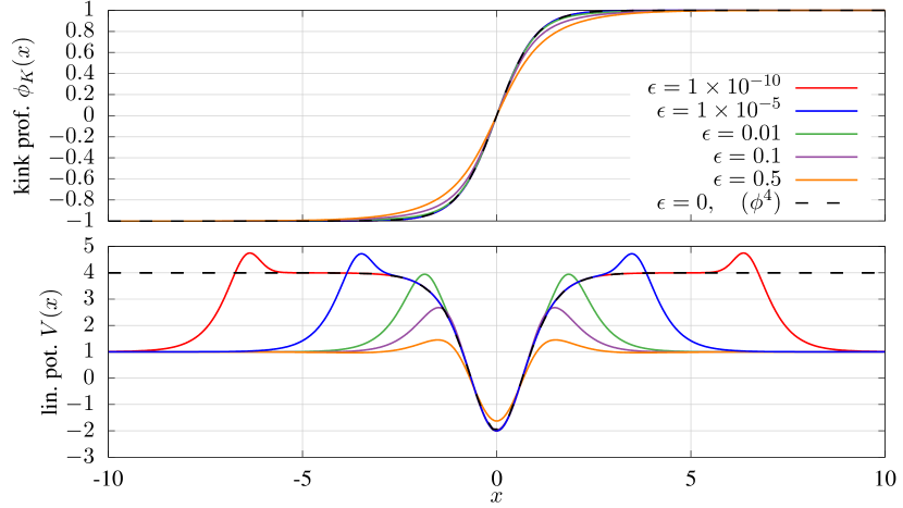
Figure 2: Profiles of the kinks and their linearised potentials.

Formally the QNMs satisfy the same linearised equation as oscillational modes. However the boundary conditions are different. For $\phi=\phi_{K}+e^{i\omega t}\eta(x)$ we require that far away from the kink

$$\eta(x)\to e^{-ik|x|},\qquad k=\sqrt{\omega^{2}-m^{2}}.$$ (15)

This condition cannot be fulfilled for real frequencies, and complex frequencies $\omega=\Omega+i\Gamma$ must be used. The imaginary part $\Gamma>0$, often referred to as the width, is responsible for the exponential decay of the mode, as seen in Figure 3.

We found the frequencies of the quasinormal modes using one of the simplest approaches, based on the Prony’s method [33]. We simulated the linear evolution with the excited profile of the $\phi^{4}$ oscillational mode and fitted a damped trigonometric function to the field measured at the $x=0.88$ for times $5<t<30$. The results are gathered in Table 1 and shown in Fig. 4. It is possible that higher QNM exist, but only the narrowest QNM contributes to the dynamics.

Figure 3: a) Exponential decay of the QNM for initial conditions $\phi(x,0)=\phi_{K}(x)+0.1\eta_{D}(x)$, $\phi_{t}(x,0)=0$ in the full nonlinear PDE. b) Profile of the QNM for different times compared with the profile of $\phi^{4}$ oscillational mode (dashed line) for linearised equation. $\epsilon=0.01$.

Table 1: Quasinormal modes frequencies

$\epsilon$	$\Omega$	$\Gamma$
0.000	1.73205	0.00000
0.001	1.75152	0.01049
0.002	1.75553	0.01559
0.005	1.76099	0.02678
0.010	1.76345	0.04075
0.020	1.76079	0.06229
0.030	1.75429	0.07975
0.050	1.73697	0.10813
0.100	1.68703	0.15922

We found that a good fit to the resonance, valid for $\epsilon<0.04$ with an accuracy of about 2%, is

$$\omega\approx 1.738+0.490\sqrt{\epsilon}-2.280\epsilon+(0.325\sqrt{\epsilon}+0.783\epsilon)i\,.$$ (16)

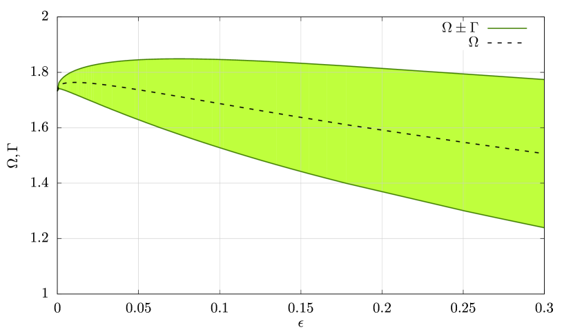
Figure 4: Quasinormal modes: frequency $\Omega$ and decay rate $\Gamma$ vs $\epsilon$.

3 Numerical results

For small values of $\epsilon$ the QNMs act very similarly to the normal, oscillational mode (NM) of the $\phi^{4}$ model: they store energy and via the resonant coupling they return it to the translational modes of the kinks. However not all the energy is given back, as some fraction of it escapes as the QNM decays exponentially. The shorter the lifetime of the QNM, the more energy escapes, and as a result bounce windows close. Our numerical simulations support this thesis, see Figures 5 and 6. The bounce windows disappear, starting from those which for $\epsilon=0$ had the largest numbers of oscillations of the internal mode and were more narrow. The windows vanish completely for $\epsilon\approx 0.033$ which corresponds to $\Gamma\approx 0.084$.

There is another interesting effect, worthy of further study. QNMs are very effective in radiating the energy from the kinks. For larger vales of $\epsilon$ one can observe that the critical velocity increases. QNM are excited but the lose energy very quickly, gluing the kink and antikink together.

We also expected that when the kinks annihilate they would form an oscillon. Surprisingly, this is not entirely true. A long-lived, almost periodic state is indeed created, but its fundamental frequency is above the $m=1$ mass threshold of the deformed theory, though still below the $\phi^{4}$ mass threshold. As a result this object radiates via its first harmonic and decays faster than a standard oscillon. Initially its decay is slow and resembles that of the $\phi^{4}$ oscillon but in time, when the amplitude decreases, the decay rate increases. We leave the detailed study of this object for future work.

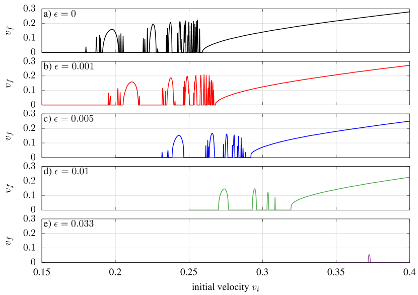
Figure 5: Final velocities of the escaping kink as a function of initial velocity for different values of $\epsilon$.

Figure 6: Scan of final velocities as a function of the initial velocity $v_{i}$ and the perturbation parameter $\epsilon$.

4 Effective model

When the resonant fractal structure was found in the $\phi^{4}$ theory, an effective model was proposed. The conjecture was that the field describing a kink-antikink collision should be described as a simple superposition of their profiles:

$$\phi(x,t)\approx\phi_{K}(x-X)-\phi_{K}(x+X)+1+\\ +\sqrt{\frac{3}{2}}A\left[\eta_{d}(x-X)-\eta_{d}(x+X)\right]$$ (17)

where $X(t)$ is the collective coordinate describing the position of the kinks and $A(t)$ is the amplitude of the oscillational modes with the profile $\eta_{d}(x)$. Substituting the above approximation into the Lagrangian and integrating one obtains an effective (mechanical) Lagrangian for $X$ and $A$. Some further approximations were used, neglecting for example anharmonic terms. After substituting (6) and integrating over spacial dimension the Lagrangian could be written in the form

$$L=a_{1}\dot{X}^{2}-a_{2}+a_{3}\dot{A}^{2}-a_{4}A^{2}+a_{5}A,$$ (18)

where the coefficients were given by appropriate integrals. This effective model gave a reasonably good approximation, reconstructing qualitatively multibounce windows, and predicting a critical velocity about 10% higher than that observed in the solution of the full PDE. Originally the coefficients (after appropriate rescaling) were given as

$$a_{1}(X)=\frac{4}{3}\left[1+\frac{6X\coth 2X-3}{\sinh^{2}2X}\right],$$ (19a)

$$a_{2}(X)=8\left[-\frac{2}{3}+2X+3\coth 2X-\right.\\ \left.-(2+6X)\coth^{2}2X+4X\coth^{3}2X\right],$$ (19b)

$$a_{3}=1,\qquad a_{4}=3,$$ (19c)

$$a_{5}(X)=-\sqrt{6}\pi\frac{\tanh^{2}2X}{\cosh^{2}2X}.$$ (19d)

Unfortunately, as pointed out in [30], the effective model had a typographic error which has been repeated in many of the following papers. The term $a_{5}$ (in literature referred to as $F(X)$) should have a different form:

$$a_{5}(X)=-3\pi\sqrt{\frac{3}{2}}\left[2-2\tanh^{3}X-\frac{3}{\cosh^{2}X}+\frac{1}{\cosh^{4}X}\right].$$ (20)

More surprisingly, the corrected version gave incorrect results, including a prediction that the resonant structure would extend to all velocities. The cure found in [30] was to take into account all the terms without any approximations. The full effective model had a further problem in that the equations were singular for $X=0$, requiring an additional term to be introduced to regularize the system of ODEs.

We decided to take the advantage of the simplicity of the original model (19) and treat it as some sort of toy or phenomenological model. The appropriate equations of motion, neglecting higher terms in $A$, can be written as

$$\ddot{X}=\frac{1}{2a_{1}}\left(a_{1}^{\prime}\dot{X}^{2}-a_{2}^{\prime}+a_{5}^{\prime}A\right),$$ (21a)

$$\ddot{A}+\Omega^{2}A-\frac{1}{2}a_{5}=0$$ (21b)

where the source term for $a_{5}$ is given by the equation (19d).

We have adapted this method for our purposes. Our model differs very little from $\phi^{4}$ for small values of $\epsilon$. The asymptotic profiles of the kinks are different but since in the original and our model they decay exponentially fast, the actual profiles of the tails do not contribute much to the collision process, especially for the large velocities that we deal with. The important modification is the change in the nature of the oscillational mode which now becomes the quasinormal mode. We leave the frequency $\Omega\approx\omega_{d}$ but we add an additional damping term to the equation for $A(t)$ describing the decay of the mode

$$\ddot{A}+2\Gamma\dot{A}+\Omega^{2}A-\frac{1}{2}a_{5}=0.$$ (22)

The width of the QNM was approximated from the fit $\Gamma\approx 0.325\sqrt{\epsilon}$. With this technique we have found that the value of $\epsilon$ for which the resonant structure vanishes is $\epsilon_{cr}=0.015$, which is a little less than half the value $\epsilon_{cr}=0.033$ found from the numerical solution of the full PDE. The results are shown in Figure 7. The resonance windows are again shifted towards higher velocities, but these shifts are rather smaller in the effective model than in the full theory, as can be seen by comparing Figures 7 and 6.

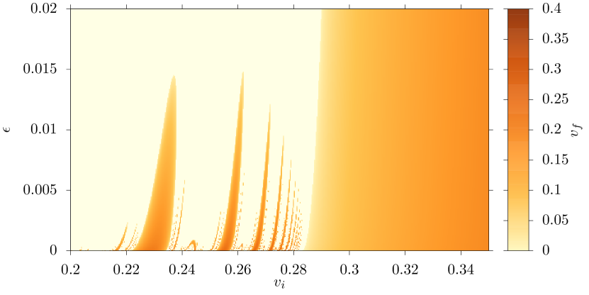
Figure 7: Scan of final velocities $v_{f}$ in the modified effective model as a function of the initial velocity $v_{i}$ and the perturbation parameter $\epsilon$.

Note that our modification does not include the change of the real part of the frequency of the QNM mode. Moreover the profile of the QNM is a complex function. Because of the radiation tails, the QNM can interact at large distances. However, our modification qualitatively reproduces the results seen in solutions of the full PDE, and we believe it will be a good starting-point for further investigations.

5 Comparison with other models

To the best of our knowledge this is the first report concerning the role of QNMs in kink collisions. One of our results is that the resonant structure of bounces can be preserved for narrow resonances. In addition we found that the critical frequency increases as the width of the resonance becomes larger. This can be explained by the fact that the collision excites the QNM, which itself quickly gets rid off energy. However it is also important that the collision excites the QNM. Over the years, many models have been studied in the context of colliding solitons, and it might be interesting to correlate the critical velocities in other models with the existence of QNM.

It is known that neither sine-Gordon (sG) nor the $\phi^{4}$ models have QNM. The linearised potentials for these two models are reflectionless Pöschl-Teller potentials. Moreover the sG model is integrable, and there is no energy exchange between the scattering modes and the solitons. The critical velocity is exactly 0 – the kinks always separate after the collision. For the $\phi^{4}$ model the critical velocity is $v_{cr}=0.26$ but the first window opens for $v=0.18$. So in a sense the oscillational mode prevents the kinks from separating for $0.18<v<0.26$.

Collisions in the $\phi^{6}$ model also have a resonant structure. However a different mechanism takes place in this model. For certain kink configurations, when the vacuum with smaller mass lies between the two kinks, some separation dependent modes could be trapped between the solitons. On the contrary when the kinks collided with the opposite arrangement the collision did not show any windows. However the critical frequency was more than six times higher, $v_{cr}=0.289$. There are known solutions to the linearised problem [34]. To calculate the position of QNM it is enough to know the asymptotic form of the solutions:

$$\begin{cases}\eta_{+\infty}(x)\to e^{-ikx},\\ \eta_{-\infty}(x)\to A(-q,-k)e^{-iqx}+A(q,-k)e^{iqx}\end{cases}$$ (23)

with

$$\begin{gathered}q=\sqrt{\omega^{2}-1},\;k=\sqrt{\omega^{2}-4},\\ A(q,k)=\frac{\Gamma(1-ik)\Gamma(-iq)}{\Gamma(-\frac{1}{2}ik-\frac{1}{2}iq+\frac{5}{2})\Gamma(-\frac{1}{2}ik-\frac{1}{2}iq-\frac{3}{2})}.\end{gathered}$$ (24)

The condition for the purely outgoing wave is that the reflection coefficient $A(q,-k)/A(-q,-k)$ has a pole. From the above form it is straightforward to obtain the positions of the poles:

$$\omega_{n}=2i\sqrt{\frac{(n+4)!}{(5+2n)^{2}n!}},\qquad n=0,1,2,\ldots$$ (25)

Note that all of the poles are on the imaginary axis. These are not unstable modes because the stability of the kink solution is guaranteed by energy arguments and the topological charge.

The nonintegrable double sine-Gordon model was studied in [3]. For certain values of parameter $-1/4<\eta<0$ it was shown that no oscillational modes exist, and a resonant structure was not found. Two critical velocities were reported: $v_{cr}(\eta=-0.05)=0.112$ and $v_{cr}(\eta=-0.15)=0.390$. For the value $\eta=-0.05$ there are no signs of QNM in the spectrum presented in [25]. If a QNM exists it is either very wide or is located below the mass threshold. On the other hand, for $\eta=-0.15$ there is a QNM with the frequency $\omega=1.078+0.499i$, and it would be particularly interesting to explore this case further in the light of the findings of the present paper.

An important question regarding the problem of increasing the critical velocity is how much the quasinormal modes get excited. If during collisions such modes are only marginally excited, their contribution to the critical velocity would be negligible even if their life-times were large.

6 Conclusions

We have shown that the well-known fractal structure of multiple bounce windows can be seen in models which neither have kinks with oscillational modes, nor kinks and antikinks forming trapping potentials. Narrow quasinormal modes can play a similar role to the oscillational modes. There is however an important difference. QNM decay exponentially, leading to energy leakage from the colliding kinks. As the width of the QNM grows, the windows close, and we have found the largest value of the QNM width which allowed for the formation of a bounce window. A further effect of the QNM is that the kinks need more kinetic energy to separate due to the increased energy leakage, and we observed that the critical velocity increased as the imaginary part of the QNM frequency increased. We have considered an effective model which differed from the standard effective model for the $\phi^{4}$ theory by a damping term in the equation describing the evolution of the mode, finding that the value of the damping term corresponded well with the width of the QNM for the upper limit allowing the bounce windows. The additional term was responsible for the increase of the critical velocity.

It is worth mentioning that a very similar problem can be addressed in a two component model when the $\phi^{4}$ field is coupled with a second second field with smaller mass. The oscillational mode from the $\phi^{4}$ field can radiate through the second channel becoming a quasinormal mode. A similar feature was pointed out in [35].

In physics there are many objects which do not have bound or oscillational modes but do have resonance modes. To name one example, the skyrmions describing nucleons have resonances discovered by Roper [36]. Such resonances can also influence the process of soliton collision, and the model that we have proposed in this paper could serve as a useful toy example for such more-complicated situations.

References

References

- [1] T. Sugiyama, Kink - antikink collisions in the two-dimensional model, Prog. Theor. Phys. 61 (1979) 1550–1563. doi:10.1143/PTP.61.1550.
- [2] D. K. Campbell, J. F. Schonfeld, C. A. Wingate, Resonance structure in kink-antikink interactions in theory, Physica D: Nonlinear Phenomena 9 (1) (1983) 1 – 32. doi:10.1016/0167-2789(83)90289-0.
- [3] M. Peyrard, D. K. Campbell, Kink-antikink interactions in a modified sine-Gordon model, Physica D Nonlinear Phenomena 9 (1983) 33–51. doi:10.1016/0167-2789(83)90290-7.
- [4] P. Anninos, S. Oliveira, R. A. Matzner, Fractal structure in the scalar theory, Phys. Rev. D44 (1991) 1147–1160. doi:10.1103/PhysRevD.44.1147.
- [5] R. H. Goodman, R. Haberman, Kink-antikink collisions in the equation: The n-bounce resonance and the separatrix map, SIAM J. Applied Dynamical Systems 4 (2005) 1195–1228. doi:doi.org/10.1137/050632981.
-
[6]
J. Yang, Y. Tan,
Fractal structure
in the collision of vector solitons, Phys. Rev. Lett. 85 (2000) 3624–3627.
doi:10.1103/PhysRevLett.85.3624.
URL https://link.aps.org/doi/10.1103/PhysRevLett.85.3624 - [7] A. Halavanau, T. Romańczukiewicz, Ya. Shnir, Resonance structures in coupled two-component model, Phys. Rev. D86 (2012) 085027. arXiv:1206.4471, doi:10.1103/PhysRevD.86.085027.
- [8] A. Alonso-Izquierdo, Reflection, transmutation, annihilation and resonance in two-component kink collisionsarXiv:1711.10034.
- [9] A. Alonso-Izquierdo, Kink dynamics in a system of two coupled scalar fields in two space-time dimensionsarXiv:1711.08784.
-
[10]
R. H. Goodman, R. Haberman,
Interaction
of sine-gordon kinks with defects: the two-bounce resonance, Physica D:
Nonlinear Phenomena 195 (3) (2004) 303 – 323.
doi:https://doi.org/10.1016/j.physd.2004.04.002.
URL http://www.sciencedirect.com/science/article/pii/S0167278904001678 -
[11]
Z. Fei, Y. S. Kivshar, L. Vázquez,