Optical solitons in periodically managed PT-symmetric media

Abstract

The dynamics of light beams in the nonlinear optical media with periodically modulated in the longtidunal direction parity-time distribution of the complex refractive index is investigated. The possibility of dynamical stabilization of PT-symmetric solitons is demonstrated.

1 Introduction

Investigation of nonlinear optical wave phenomena in media with the parity-time symmetry properties of the complex spatially modulated refraction index attracts a great attention last time [1, 2]. Mainly it is related with the important properties of the systems with non-Hermitian hamiltonian with PT-symmetry. Such systems for values of the gain/loss parameter lower than critical values have real eigenvalues [3]. This phenomenon has direct analogies in the optical systems. For example in the paraxial approximation the wave equation for electromagnetic waves has the form of the Schrödinger equation with the spatial distribution of the gain/loss parameters. The PT symmetry constrain leads to the existence of the stationary modes in the non-conservative optical systems. In nonlinear optical media described by the PT-symmetric extended nonlinear Schrödinger equation it leads to the existence of families of optical solitons [4, 5]. Now a great interest has been attracted to management of solitary waves in media with parity-time invariant properties. In particular the periodically modulated optical systems with balanced gain and loss has been studied in [6], where in the high frequency limit an effective PT-symmetric system has been obtained from initially non - PT symmetric optical system. Note the periodic variation in the longitudinal direction (LD) involving the real part of the refractive index was considered there. Another possibility is to consider periodic variations in the longitudinal direction, involving also the imaginary part of the refractive index, i.e. the imaginary part of the potential $V_{I}$ in the corresponding Schrödinger equation. These possibilities are investigated in the nonlinear directional coupler with periodically modulated gain/loss along LD [7, 8]. The stabilization of nonlinear modes has been found. The considered problem can be called as the imaginary Kapitza problem. In the work [9] a linear Schrödinger equation with oscillating imaginary Gaussian potential has been investigated. It was shown that in the HFL the spectrum of quasi-energy is real valued leading to the existence of stationary modes. The results have applications to the stability of optical resonators with variable reflectivity. Another example is the BEC with spatially distributed gain//loss parameters, described by the Gross-Pitevskii equation with PT symmetric potential [10]. It is of interest to study the imaginary Kapitza problem for the case of nonlinear optical media. We will consider dynamics of solitons in media with the Kerr nonlinearity with rapidly managed PT-symmetric potential. In particular we will study the possibility of stabilization of unstable nonlinear modes.

The paper is organized as follows: In section 2 we formulate the model and describe the procedure of obtaining averaged equation for the GP equation with a PT-potential being periodically varied in the longthidunal direction and inhomogeneous in space. The results of numerical simulations of the full and averaged NLS equations for optical soliton propagation are presented in section 3.

2 The model: Averaged NLS equation

Let us consider propagation of a light in the nonlinear media with modulated in the space complex refraction index. In the parabolic approximation the electric field propagation is described by the wave equation [11]:

$$2ik_{0}n_{0}E_{Z}+E_{xx}+2k_{0}^{2}n_{0}\Delta n(x,z)E+2k_{0}^{2}n_{0}n_{2}|E|^{2}E=0,$$ (1)

where $k_{0}=2\pi/\lambda$, $\Delta n(x,z)=n_{R}(x)+in_{I}(x,z)$ is the complex refraction index. Introducing dimensionless variables

$$t=Z/L_{d},x=X/w_{0},u=(k_{0}|n_{2}|L_{d})^{1/2}E,\ U(x,z)=-k_{0}L_{d}\Delta n(x,z),$$

where $L_{d}=k_{0}n_{0}w_{0}^{2}$ is the diffraction length, $w_{0}$ is the beam initial width , we obtain the following wave equation:

$$iu_{t}+u_{xx}-V(x,t)u+2|u|^{2}u=0.$$ (2)

Analogous equation also describes dynamics of BEC with attractive interaction in the complex trap potential, namely, the time dependent GP equation

$$i\hbar\psi_{\tau}=-\frac{\hbar^{2}}{2m}\Delta\psi+V_{tr}(r,t)\psi+g|\psi|^{2}\psi,$$ (3)

where $m$ is the atom mass, $g=4\pi\hbar^{2}a_{s}/m$ and $a_{s}$ is the atomic scattering length. $a_{s}>0$ corresponds to the BEC with repulsive interaction between atoms and $a_{s}<0$ to the attractive interaction. We restrict ourselves by considering a cigar-shaped condensate that allows us to deal with a quasi 1D mathematical model (2). The complex trap potential in BEC has been realized recently in [12].

We will consider next model of time modulated potential.

$$V(x,t)=\alpha(t)V_{PT}(x).$$

The another possible model is with modulation in time of the imaginary part of the potential

$$V(x,t)=V_{R}(x)+i\alpha(t)V_{I}(x),$$

can also be described by considering in this work method. We come to the following governing equation

$$iu_{t}+u_{xx}-\alpha(t)V_{PT}(x)u+2|u|^{2}u=0,$$ (4)

where $V_{PT}(x)$ is a PT- symmetric potential in $X,t$-space, $\alpha(t)$ describes the time modulations of the potential. $V_{PT}(x)=f(x)$ is a complex function with even real and odd imaginary parts, $\alpha(t)=\alpha_{0}+\gamma(t)$. The modulation of potential is supposed to be periodic in time

$$\gamma(t+T)=\gamma(t),\ \ \ \int_{0}^{T}\gamma(t^{\prime})dt^{\prime}=0.$$ (5)

Temporal modulation is chosen as

$$\gamma(t)=\alpha_{1}\cos(\Omega t).$$ (6)

We suppose the modulation frequency $\Omega$ to be large ($\Omega\gg 1$). Thus in our problem a value $\epsilon=\alpha_{1}/\Omega$ emerges which is a characteristic of the potential strength modulation and the frequency of rapid oscillations.

2.1 Small strength of the trap perturbation $\epsilon=O(0)$

The field $u(x,t)$ can be represented in the form of sum of slowly and rapidly varying parts $U(x,t)$ and $\xi(x,t)$

$$u(x,t)=U(x,t)+\xi(x,t).$$ (7)

For obtaining equation for the averaged field $u(x,t)$ we will present the rapidly varying part of the field as a Fourier series expansion [13, 14]:

$$\xi=A\cos(\Omega t)+B\sin(\Omega t)+C\cos(2\Omega t)+D\sin(2\Omega t)+...\ ,$$ (8)

where $A,B,C$ and $D$ are slowly varying in time small functions of variables $x$ and $t$ of the order $O(1)$. By substituting equations (7) and (8) into (4) we obtain the next set of equations for the slowly varying field $U$ and coefficients of the expansion of the rapidly varying component

$$iU_{t}+U_{xx}+2|U|^{2}U+2U(|A|^{2}+|B|^{2}+|C|^{2}+|D|^{2})+$$

$$U^{*}(A^{2}+B^{2}+C^{2}+D^{2})+A^{*}BD+AB^{*}D+ABD^{*}+$$

$$C(|A|^{2}-|B|^{2})+\frac{1}{2}C^{*}(A^{2}-B^{2})=\alpha_{0}f(x)U+\frac{\alpha_{1}}{2}f(x)A,$$ (9)

$$iA_{t}+i\Omega B+A_{xx}+4|U|^{2}A+2U(AC^{*}+A^{*}C+BD^{*}+B^{*}D)+$$

$$2U^{*}(AC+BD)+2U^{2}A^{*}+A\left(\frac{3}{2}|A|^{2}+|B|^{2}+2|C|^{2}+2|D|^{2}\right)+$$

$$A^{*}\left(\frac{1}{2}|B|^{2}+|C|^{2}+|D|^{2}\right)=\alpha_{0}f(x)A+\frac{\alpha_{1}}{2}f(x)C+\alpha_{1}f(x)U,$$ (10)

$$iB_{t}-i\Omega A+B_{xx}+4|U|^{2}B+2U(AD^{*}+A^{*}D-BC^{*}-B^{*}C)+$$

$$2U^{*}(AD-BC)+2U^{2}B^{*}+B\left(|A|^{2}+\frac{3}{2}|B|^{2}+2|C|^{2}+2|D|^{2}\right)+$$

$$B^{*}\left(\frac{1}{2}|A|^{2}+|C|^{2}+|D|^{2}\right)=\alpha_{0}f(x)B+\alpha_{1}f(x)D,$$ (11)

$$iC_{t}+2i\Omega D+C_{xx}+4|U|^{2}C+2U(|A|^{2}-|B|^{2})+$$

$$U^{*}(A^{2}-B^{2})+2U^{2}C^{*}+C\left(2|A|^{2}+2|B|^{2}+\frac{3}{2}|C|^{2}+|D|^{2}\right)+$$

$$C^{*}\left(|A|^{2}+|B|^{2}+\frac{1}{2}|D|^{2}\right)=\alpha_{0}f(x)C+\frac{\alpha_{1}}{2}f(x)A,$$ (12)

$$iD_{t}-2i\Omega C+D_{xx}+4|U|^{2}D+2U(AB^{*}+A^{*}B)+$$

$$2U^{*}AB+2U^{2}D^{*}+D\left(2|A|^{2}+2|B|^{2}+|C|^{2}+\frac{3}{2}||D|^{2}\right)+$$

$$D^{*}\left(A^{2}+B^{2}+\frac{1}{2}C^{2}\right)=\alpha_{0}f(x)D+\frac{\alpha_{1}}{2}f(x)B.$$ (13)

The parameter $\Omega$ is supposed to be $\gg 1$. Then we can introduce a small parameter $\epsilon=1/\Omega$. Considering Eq. (2.1) and neglecting all small terms of the order of $O(\epsilon^{2})$ we come to

$$iB+O(\epsilon^{2})=\frac{\alpha_{1}}{\Omega}f(x)U+O(\epsilon^{2}).$$

So we have solution for unknown $B$

$$B=-i\epsilon\alpha_{1}f(x)U.$$ (14)

Thus structure of equations (2.1 - 2.1) allows to suppose that

$$B\approx\epsilon,\ \ A\approx\epsilon^{2},\ \ C\approx\epsilon^{2},\ \ D\approx\epsilon^{3}.$$

The rest of parameters $A$ and $C$ are

$$A=-i\epsilon^{2}\alpha_{1}f(x)U_{t}-\epsilon^{2}\alpha_{1}(f(x)U)_{xx}-2\epsilon^{2}\alpha_{1}f(x)|U|^{2}U+\epsilon^{2}\alpha_{0}\alpha_{1}f^{2}(x)U,$$

$$C=\epsilon^{2}{\alpha_{1}}^{2}\frac{f^{2}(x)}{4}U.$$ (15)

Let’s consider Eq. (2.1). Holding only terms of order $\epsilon^{2}$ the equation becomes

$$iU_{t}+U_{xx}+2|U|^{2}U+2U|B|^{2}+U^{*}B^{2}=\alpha_{0}f(x)U+\frac{\alpha_{1}}{2}f(x)A.$$ (16)

Substituting expressions for $A,B,C$ from (14), (2.1) into Eq. (16), we obtain an averaged equation for $U$

$$iU_{t}+U_{xx}+2|U|^{2}U+2\epsilon^{2}{\alpha_{1}}^{2}|f(x)|^{2}|U|^{2}U-\epsilon^{2}{\alpha_{1}}^{2}f^{2}(x)|U|^{2}U=$$

$$\alpha_{0}f(x)U-i\frac{\epsilon^{2}}{2}{\alpha_{1}}^{2}f(x)U_{t}-\frac{\epsilon^{2}}{2}{\alpha_{1}}^{2}f(x)(f(x)U)_{xx}-$$

$$\epsilon^{2}{\alpha_{1}}^{2}[2f(x)-f^{*}(x)]f(x)|U|^{2}U+\frac{\epsilon^{2}}{2}{\alpha_{1}}^{2}\alpha_{0}f^{3}(x)U.$$ (17)

Hereafter we redesignate $\epsilon=\alpha_{1}/\Omega$. Then introducing new field $V(x,t)$

$$\tilde{U}(x,t)=\left(1+\frac{\epsilon^{2}}{2}f^{2}(x)\right)^{1/2}U(x,t),$$ (18)

into Eq. (2.1) we have finally the following equation

$$i\tilde{U}_{t}+\tilde{U}_{xx}+2(1+G_{eff})|\tilde{U}|^{2}\tilde{U}=W_{eff}(x)\tilde{U}.$$ (19)

The averaged equation is a modified NLS equation with an effective slowly varying linear and nonlinear potentials

$$\ W_{eff}(x)=\alpha_{0}f(x)+\frac{\epsilon^{2}}{2}f^{2}_{x}(x),\ 2G_{eff}|\psi|^{2}=2\left(1+\epsilon^{2}(Imf(x))^{2}\right)|\tilde{U}|^{2}.$$ (20)

2.2 Strong management

Let us consider for simplicity the case of pure imaginary potential ($V_{R}=0$). To investigate the dynamics of beam in the case of strong management it is useful to perform transformation of the field

$$u(x,t)=U(x,t)e^{-\Gamma(t)V_{I}(x)},$$ (21)

where $\Gamma(t)$ is the antiderivative for $\gamma(t)$

$$\Gamma(t)=\int_{0}^{t}\gamma(t^{\prime})dt^{\prime}.$$

Here we assume that field $U(x,t)$ is slowly varying on the period of oscillations of complex potential. We will check the consistency of this assumption s by the multiscale perturbation theory below. Substituting this expression into Eq. (2.1) we obtain the equation for $U(x,t)$:

$$iU_{t}+U_{xx}-2U_{x}\Gamma V_{I,x}-U\Gamma V_{I,xx}+U\Gamma^{2}V_{I,x}^{2}+2|U|^{2}Ue^{-2\Gamma V_{I}(x)}=0$$ (22)

Let us consider the case of periodic modulations

$$\gamma(t)=\gamma_{0}\cos(\omega t).$$

and the management is strong i.e. $\gamma_{0},\omega\gg 1,\gamma_{0}/\omega=O(1)$. Averaging this equation over period of modulations we have averaged equation

$$iU_{t}+U_{xx}+\frac{\gamma_{0}^{2}}{2\Omega^{2}}V_{I,x}^{2}U+2I_{0}(\frac{2\gamma_{0}}{\Omega}V_{I}(x))|U|^{2}U=0.$$ (23)

Here we take $<\Gamma>=0,\ <\Gamma^{2}>=\gamma_{0}^{2}/2\omega^{2},\ <...>=\frac{1}{T}\int_{0}^{T}(...)dt,\ T=2\pi/\omega$. $I_{0}(x)$ is the modified Bessel function of the first kind

$$I_{0}(x)=\frac{1}{2\pi}\int_{0}^{2\pi}e^{x\sin(t)}dt.$$

From this averaged equation we can now conclude that dynamics is described now by conservative modified NLS equation with the effective linear potential

$$-\frac{\gamma_{0}^{2}}{2\Omega^{2}}V_{I,x}^{2}$$

and the effective nonlinear potential induced by spatially varying Kerr nonlinearity

$$I_{0}[\frac{2\gamma_{0}}{\Omega}V_{I}(x)]>1.$$

Considering the case of weak management when $2\gamma_{0}/\Omega\ll 1$ and expanding in Eq. (23) coefficients in power series we obtain the averaged equation Eq. (19) for the weak management case.

3 Numerical results

In numerical simulations we use the following PT potential which was used in the works [15]

$$V_{PT}(x)=-V_{0}\mbox{sech}^{2}(x)-W_{0}\sinh(x)\mbox{sech}^{2}(x),$$ (24)

Soliton solution to the standard Gross-Pitaevskii equation

$$iu_{t}+u_{xx}-V_{PT}(x)u+2|u|^{2}u=0,$$ (25)

with potential (24) has the form [4]

$$u_{s}(x,t)=\frac{u_{0}}{\sqrt{2}}\mbox{sech}(x)\exp(i\mu\arctan(\sinh(x))\exp(i\lambda t),$$ (26)

where the solution parameters $\lambda=1,\ \ \ \mu=W_{0}/3$ and $\ \ u_{0}=\left(2-V_{0}+\mu^{2}\right)^{1/2}.$ As known from the work [15] PT-potential Eq. (24) in linear problem exhibits real spectrum provided that $W_{0}\leq V_{0}+1/4$. In other words it means that otherwise the potential leads to unstable solutions of equation  (25).

First we studied travelling of solitons through imaginary PT-potential Eq. (24) (supposing $V_{0}$ to be zero). We considered the NLS soliton having the form

$$u_{sol}(x,t)=A\mbox{sech}\left(A(x-vt)\right)\exp\left(i(vx/2+(A^{2}-v^{2}/4)t)\right).$$ (27)

Fig. 1 depicts dynamics of a NLS soliton being scattered by this PT-potential. The soliton of the norm $N=2.5$ incident on the PT-potential moves with the velocity $v=0.4$. The PT potential Eq. (24) with $V_{0}=0$ and $W_{0}=1.5$ is under action of temporal modulation. Parameters of the modulation in full equation (4) are $\alpha_{0}=0,\ \ \alpha_{1}=36$ and $\Omega=120$ that correspond to modulation parameter $\epsilon=0.3$ in averaged equation (19). One can see that the travelling soliton keeps ideally its form in the course of all its movement. Averaged dynamics of the wave function amplitude is depicted in Fig. 2. Left panel shows that amplitude makes a jump as the soliton passes the potential center. Solid line is for averaged solution of full equation (4), dot line is for solution of averaged equation (19) Non-averaged and averaged amplitudes of full equation (4) is shown in the right panel.

Figure 1: Evolution of the NLS soliton profile when travelling through the imaginary PT-potential.

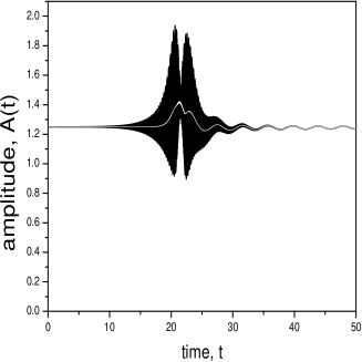
Figure 2: Evolution of the NLS soliton amplitude: left panel shows averaged amplitude of full equation (solid line) and amplitude of averaged equation (dot line). Right panel depicts non-averaged (black line) and averaged (white line) amplitudes of full equation.

Next we studied averaged dynamics of the soliton solution Eq. (26) under action of strong strength modulation of PT-potential Eq. (24). In the case of strong management the results of full numerical simulations were compared with the ones of simulation of the averaged equation Eq. (23). In calculations $\alpha_{0}=1,\ \alpha_{1}=52.5,\Omega=70$ that matches to $\epsilon=0.75$. Figure 3 depicts oscillations of the soliton amplitude when initial position of the soliton is shifted and $x_{0}=-0.2$. The zero value $x_{0}=0$ corresponds to a stationary soliton solution. Parameters of the potential Eq. (24) $V_{0}=1,\ \ W_{0}=1.5$. In such a choice of parameter values imaginary part $W_{0}$ is above the PT threshold where a phase transition occurs and the spectrum enters the complex domain i.e. the soliton solution becomes unstable. Here two solutions are presented, averaged solution of the equation Eq. (4) with rapidly varied strength of potential Eq. (24) and solution of the averaged equation Eq. (23) with the effective potential .

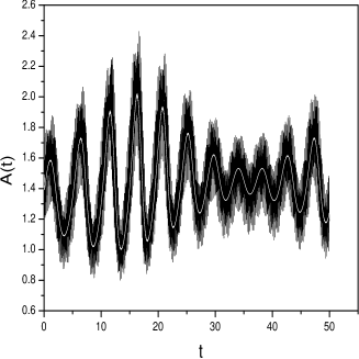
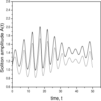
Figure 3: Left panel: Time Dependence of the amplitude of the full equation solution (black line) and the averaged one (white line). Right panel: The dependence of the averaged amplitude of the full equation solution on time (bold line) and amplitude of averaged equation (dot line). PT soliton parameters are $V_{0}=1,W_{0}=1.5,\epsilon=0.75$.

Figure 4 shows the soliton amplitude evolutions when rapid perturbations of the PT-potential Eq. (24) are turned off and so $\epsilon=0$ (solid line) and the case with temporal modulations at $\epsilon=0.4$ (dot line). Parameters of the potential Eq. (24) are $V_{0}=1,\ \ W_{0}=1.5$. As seen when $\epsilon=0$ the solution amplitude diverges ($W_{0}>V_{0}+1/4$ in linear case) and the potential spectrum has complex domain. Applying external modulation suppress the divergence.

Figure 4: The soliton amplitude evolution when rapid oscillations of the potential is turned off, i.e. $\epsilon=0$ (solid line) and evolution at $\epsilon=0.4$ (dot line), i.e. modulation is turned on. PT potential parameters are $V_{0}=1,\ W_{0}=1.5,\ \alpha_{0}=1,\ \alpha_{1}=48,\ \Omega=120.$

Convergence of the parameter $\epsilon$ by the modulation frequency variation is shown in Fig. 5. Note that curves for $\Omega=70$ and $\Omega=120$ coincide.

Figure 5: The soliton amplitude evolutions are depicted at $\epsilon=0.3$ with different rapid oscillations of the potential. PT potential parameters are $V_{0}=1,\ W_{0}=1.5,\ \alpha_{0}=1,\ \alpha_{1}/\Omega=9/30\ ,21/70\ ,36/120$, respectively dash, solid, solid lines.

4 Conclusion

In conclusion we investigate the dynamics of optical solitons in the media with rapidly varying PT-symmetric distribution of the complex refractive index. We derive modified nonlinear Schrodinger equation to describe averaged dynamics of optical solitons. Two cases with the weak and strong managements of the complex refraction index have been considered. In description of the dynamics, the management results in appearance of effective modified linear potential and spatially varying effective Kerr nonlinearity in the NLSE, depending on the ratio of the amplitude and the frequency of modulations. We study propagation of the NLS soliton through oscillating PT-potential and found that the norm of the soliton makes a jump when passing the potential, keeping ideally its form. In the case of strong management $\epsilon\neq 0$ and when $W_{0}>V_{0}+1/4$ (trap potential spectrum has complex domain) we observe that strong management turns off the divergence of the soliton dynamics being observed at $\epsilon=0$, i.e. we observe the dynamical stabilization phenomena. It has been theoretically and numerically shown that two parameters $\alpha_{1}$ and $\Omega$ form a single parameter $\epsilon=\alpha_{1}/\Omega$. These effects open new possibilities for the control and steering of the optical beams.

References

• [1] V. V. Konotop, J. Yang, and D. A. Zezyulin, Rev. Mod. Phys. 88 (2016) 035002.
• [2] S. V. Suchkov, A. A. Sukhorukov, J. Huang, S. V. Dmitriev, C. Lee, Yu. S. Kivshar, Laser & Photonics Reviews, 10 (2016) 177.
• [3] C. M. Bender and S. Boettcher, Phys. Rev. Lett. 80 (1998) 5243–5246.
• [4] Z.H.Musslimani, K.G.Makris, R. El-Ganainy, and D.N. Christodoulides, Phys.Rev Letters 100 (2008) 030402.
• [5] F. K. Abdullaev, Y. V. Kartashov, V. V. Konotop, and D. A. Zezyulin, Phys. Rev. A 83 (2011) 041805.
• [6] X. B. Luo, J. H. Huang, H. H. Zhong, X. Z. Qin, Q. T. Xie, Y. S. Kivshar, and C. H. Lee, Phys. Rev. Lett. 110 (2013) 243902.
• [7] R. Driben and B. A. Malomed, Europhys. Lett. 96 (2011) 51001.
• [8] R. L. Horne, J. Cuevas, P. G. Kevrekidis, N. Whitaker, F. K. Abdullaev, and D. J. Frantzeskakis, J. Phys. A 46 (2013) 485101–19.
• [9] B. Torosov, G.Della Valle, and S. Longhi, Phys. Rev. A 88 (2013) 052106.
• [10] H. Cartarius and G. Wunner, Phys. Rev. A 86 (2012) 013612.
• [11] Yu. S. Kivshar, G.P. Agrawal, Optical Solitons: From Fibers To Photonic Crystals, Academic Press, San Diego, 2003.
• [12] R. Stützle, M. C. Göbel, Th. Hörner, E. Kierig, I. Mourachko, M. K. Oberthaler, M. A. Efremov, M. V. Fedorov, V. P. Yakovlev, K. A. H. van Leeuwen, and W. P. Schleich Phys. Rev. Lett. 95 (2005) 110405.
• [13] Y.S. Kivshar, K.H. Spatschek Chaos, Solitons and Fractals 5, (1995), 2551-2569.
• [14] F.Kh. Abdullaev, R.M. Galimzyanov J.Phys B 36,(2003), 1099-1108.
• [15] Z. Ahmed, Phys. Lett. A 282 (2001) 343-348.