An Unsupervised Homogenization Pipeline for Clustering Similar Patients using Electronic Health Record Data

Abstract

Electronic health records (EHR) contain a large variety of information on the clinical history of patients such as vital signs, demographics, diagnostic codes and imaging data. The enormous potential for discovery in this rich dataset is hampered by its complexity and heterogeneity.

We present the first study to assess unsupervised homogenization pipelines designed for EHR clustering. To identify the optimal pipeline, we tested accuracy on simulated data with varying amounts of redundancy, heterogeneity, and missingness. We identified two optimal pipelines: 1) Multiple Imputation by Chained Equations (MICE) combined with Local Linear Embedding; and 2) MICE, Z-scoring, and Deep Autoencoders.

I Introduction

Doctors provide diagnoses to help predict the health trajectory of their patients. A diagnosis also helps to predict what treatments have the highest likelihood of improving a patient’s health. The more granular the diagnosis, the more specific or “precise” medicine can become. The wealth of medical data gathered from patients, that is digitally available in an electronic health record (EHR), should support highly granular diagnoses. Unfortunately, the current clinical paradigm of a human physician wading through this vast sea of data cannot deliver the promise of precision medicine.

Fortunately, advances in machine learning can be harnessed to sift through this rich dataset and extract useful information to facilitate human decisions. One popular application is phenotyping by cluster analysis. Previous studies [1, 2, 3] have shown that clustering algorithms have the potential to classify patients into similar phenotypes based on data contained in the medical record. For example, using unbiased hierarchical cluster analysis and penalized model-based clustering, Shah et al. [2] identified 3 phenotypes in patients diagnosed with heart failure with preserved ejection fraction. Upon identification of such granular and more homogeneous clusters, the outcomes (e.g. hospitalization, cardiac events or mortality) and attempted therapies within each cluster can then be linked together to predict likely outcomes resulting from choosing particular therapies.

While there have been many advances in the field of cluster analysis [4], the methods rely on the assumption of homogeneous, non-redundant and complete data. However, EHR data are heterogeneous (variables can be continuous or categorical, and with different scales), redundant (multiple measurements may assess the same underlying patient feature), incomplete (many fields in the clinical reports are sparsely filled depending on the purpose of the study), and noisy (not all variables are informative in all conditions). Additionally, human errors and system biases also contribute to measurement errors in EHR data. Thus, to fully utilize the EHR to reliably detect disease subtypes, clustering techniques must be paired with pre-processing techniques that normalize and reduce the complexity of the raw EHR data. Such a clustering pipeline, including pre-processing steps, has not been previously proposed or validated.

In this paper, we assess and propose an optimal clustering pipeline that is robust to the nuisances of EHR data. The pipeline consists of imputation, normalization, feature reduction, and clustering. Multiple commonly used techniques are evaluated at each step, and the best performing pipeline is selected. Since the accuracy of clusters in real EHR applications cannot be measured due to lack of a ground truth, we assessed accuracy using simulated EHR data where ground truth could be easily defined. To the best of our knowledge, this is the first study to propose and validate an unsupervised homogenization pipeline for EHR clustering.

II Methods

II-A EHR Data Simulation

We simulated patient encounters with a sample generator that mimics the redundancy and heterogeneity of EHR data. We defined rows for patient encounters (samples) and columns for measurements taken from the patient (features). We designed three clusters with $n$ samples per cluster, observed dimensionality $m$, and effective dimensionality of 2 (for visualization convenience).

The sample generator drew $3n$ independent samples from a multivariate normal distribution with $\mu=[0,0],$ and $\Sigma=\mathbf{I}_{2\times 2}$ to form the matrix $N_{3n\times 2}$. Then, we separated the clusters by shifting $n$ samples at a time. The first $n$ samples stayed in the origin, while the next $n$ were shifted by $[d,0]$, and the last $n$ were shifted by $[\frac{d}{2},\frac{\sqrt{3}}{2}d],$ forming an equilateral triangle with a distance $d$ from each vertex.

We emulated redundancy by projecting the original feature vector to a $m$-dimensional space: $X_{3n\times m}=N_{3n\times 2}P_{2\times m},$ where the elements of the projection matrix, $P$, were drawn from a uniform distribution in the range $(0,1).$

We then enforced heterogeneity by quantizing half of the variables (set to zero if below the mean and 1 otherwise), chosen at random, and scaling each continuous feature with a random factor between 1 and 100. Finally, we added Gaussian noise ($\mu=0,\sigma=1$) to every element in the data matrix to mimic measurement errors.

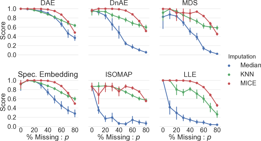
Figure 1: Missingness experiment results.

II-B EHR Clustering Pipeline

II-B1 Imputation

We tested median imputation, where the median value from valid samples complete missing values; k-Nearest Neighbors (KNN), where the average value from the k-nearest samples is used; and Multiple Imputation by Chained Equations (MICE) [5], where the missing values are predicted based on regression models with complete samples.

II-B2 Normalization

For continuous variables, we tested Z-score, where every variable is set to zero mean and unit variance; MinMax, which normalizes to a [0,1] range; and Whitening, where the feature space is linearly projected such that inter-feature covariance is the identity matrix.

II-B3 Feature reduction

We propose the use of Deep Autoencoders (DAE) [6] and Denoising Autoencoders (DnAE) [7] for EHR feature reduction. Autoencoders are trained to reconstruct an input through encoding and decoding networks. In the DnAE case, noise is added to the encoded units to enforce robustness to measurement noise.

We designed the network architechture with a hyper-parameter search for layers, hidden, and encoding units. The network with the least number of encoding units that achieves the reconstruction error of 1% or less is preferred. The encoding vectors represent EHR data in a compressed and continuous vector, suitable for any clustering technique.

For comparison, we evaluated other methods with local (Local Linear Embedding (LLE) [8]) and global neighbor algorithms (Isometric Mapping (ISOMAP) [9]); as well as affinity matrix algorithms, such as Spectral Embedding [10] and Multidimensional Scaling (MDS) [11].

II-B4 Clustering

Without loss of generality, we used K-means to conduct the final cluster analysis.

II-C Simulation Setup and Experiments

First, we simulated a baseline scenario where all parameters were set to an ideal level with complete, free of noise, $d=10$, 5000 samples per cluster, and $m=10$. An effect size of 10 resulted in less than 0.01% overlap between clusters, and heuristically $m=10$ resulted in good performance for all pipelines. This baseline was used to identify the best performing pair of normalization and feature reduction methods, which were then used in the rest of the experiments.

We then simulated four scenarios for testing the pipeline robustness at various levels of severity. In all experiments, we swept one simulation parameter while keeping all others constant. We measured the adjusted rand-score [12], which computes a similarity measure between the results of two sets of labels by counting pairs that are assigned in the same or different clusters in the predicted and true clusterings while adjusting for random chance. Table I describes each experimental setup and the default parameters. Every experiment was run 5 times to extract the mean and standard deviation of the performance.

TABLE I: Simulation experiments with default parameters $p=0$, $\eta=0$, $d=10$, $n=5000$, and $m=10$.

Experiment	Parameter	Levels
Effect Size	$d$	[3, 4, 5, 6, 7, 8]
Features	$m$	[6, 20, 40, 100, 200, 500]
Missingness (%)	$p$	[0, 10, 20, $\dots,$ 80]
Noise	$\eta$	[4, 16, 64, 128, 256]

II-C1 Missingness

To simulate the missing entries in the EHR, we randomly removed a percentage $p$, from the observed data matrix and denoted them as missing values. We varied $p$ from 0 to 80% in increments of 10%.

II-C2 Effect Size

We manipulated the effect size by varying the distance between cluster centers, $d$. In two dimensions, we can calculate the number of overlapped samples by counting the number of samples beyond a distance of $\frac{d}{2}$ in a bivariate standard normal distribution. Then, in a triangular setting, the number of overlapped samples would be 6 times the calculated amount. By conducting a Monte Carlo simulation, we can convert the effect sizes of 3–8 to the percentage of overlapped samples [13.35%, 4.55%, 1.24%, 0.27%, 0.04%, 0.01%]. This can be interpreted as the lower-bound for error in cluster assignment.

II-C3 Redundant Features

We assessed the robustness to the number of redundant features present in the dataset by increasing the dimensionality, $m$, while keeping the ground-truth dimensionality of 2. We simulated projection matrices that generated [6, 20, 40, 100, 200, 500] features.

II-C4 Uninformative/Noisy Features

EHR data contain information that may not be useful in determining clusters of similar patients. We assessed the effects of including non-informative variables by appending $\eta$ random continuous and $\eta$ random binary variables.

TABLE II: Baseline results for identifying best scaling for each feature reduction method. The entries show average score and standard deviation of the scores across repetitions.

	MinMax	Raw	Whitening	Z-score
DAE	0.982(0.03)	0.822(0.20)	0.841(0.15)	0.998(0.00)
DnAE	0.983(0.03)	0.769(0.20)	0.781(0.20)	0.998(0.00)
MDS	0.903(0.17)	0.985(0.03)	0.294(0.18)	0.999(0.00)
ISOMAP	0.264(0.41)	0.235(0.35)	0.822(0.26)	0.390(0.43)
LLE	0.737(0.20)	0.976(0.05)	0.503(0.32)	0.745(0.21)
Spec. Emb.	0.770(0.21)	0.994(0.01)	0.634(0.29)	0.753(0.23)

III Results

The baseline experiment revealed that the performance of the clustering pipeline heavily depended on the choice of normalization and feature reduction method (see Table II).DAE, DnAE, and MDS paired best with Z-scoring, all with scores above 0.99. ISOMAP performed best with Whitening while LLE and Spectral Embedding obtained its best performance when no scaling was used. We used these optimal pairs to conduct the remainder of the experiments.

III-A Robustness Experiments

III-A1 Missingness

As shown in Fig. 1, levels of missingness above 60% significantly impaired the clustering performance for all pipeline configurations (all scores below 0.8). Among the three imputation methods, MICE resulted in the best performance for all feature reduction methods except ISOMAP, for which KNN was marginally better up to 50%. Median imputation consistently the worst performance.

III-A2 Effect Size

As expected, the performance of all configurations increased with the effect size (Fig. 2(a)). Overall, the top three performing feature reduction methods were LLE, DAE, and MDS. LLE exhibited the best performance across feature reduction methods but only marginally better than DAE, e.g. the p-value of a paired t-test was 0.03 at the effect size of 4.

III-A3 Features

LLE, DAE, and MDS were essentially immune to large amounts of redundant features (Fig. 2(b)). DnAE appeared to be similarly immune at low levels, but its performance sharply decreased with greater than 200 features. Conversely, Spectral Embedding benefited from higher numbers of redundant features and performed on par to the best methods for 200 and 500 redundant features. ISOMAP performed poorly at all levels

III-A4 Uninformative/Noisy Features

As shown in Fig. 2(c), most methods, except DnAE and ISOMAP, were immune to large amounts of uninformative variables. DnAE was robust to uninformative variables up to 32 continuous and binary uninformative variables. ISOMAP did not tolerate even the minimum number of uninformative variables.

III-B Interaction Experiments

Following the robustness experiments, we identified DAE and LLE as the top 2 best performing feature reduction methods overall. To further compare these methods, we performed subsequent experiments that allowed for interactions of varying effect sizes, missingness, and noise.

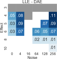
(a) Effect size vs Noise

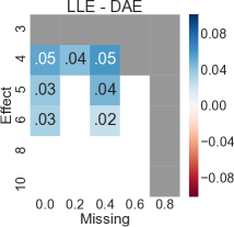
(b) Effect size vs Missingness

Figure 3: Interaction experiments. The gray areas denote where neither method scored above 0.8, the white areas denote no significant difference between score means. The colored areas denote significant differences between LLE and DAE.

Overall, LLE matched or outperformed DAE. In the effect size vs noise experiment, (Fig. 3(a)) large amounts of uninformative variables and medium effect sizes favored LLE. In the effect size vs missingness experiment, (Fig. 3(b)) LLE showed significantly better performance for medium effect sizes and low missingness and no difference for large effect sizes and low to medium missingness.

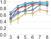
(a) Effect size $d$

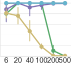
(b) Features $m$

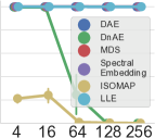
(c) Noise $\eta$

Figure 2: Robustness experiments results

IV Discussion

In the current paper, we propose and evaluate a clustering pipeline tailored for complex EHR data by comparing performances of commonly used techniques. We found two pipelines that outperform other alternatives: 1) MICE imputation + LLE feature reduction; 2) MICE imputation + Z-score normalization + DAE feature reduction. Both pipelines are robust to missingness (up to 60%), uninformative noise and large numbers of redundant features, while LLE performs slightly better at smaller effect size. This is the first study to present an unsupervised homogenization pipeline designed for EHR clustering.

Normalization

EHR data are heterogeneous, containing both categorical and continuous variables at different scales. Normalization is recommended to reduce the variance among variables. Most previous studies [2, 13, 14] normalized EHR variables to a range of (0, 1), however, as shown in Table II, the best normalization method is closely related to the feature reduction method. For example, for DAE and DnAE, Z-score normalization results in the best performing pipelines, while no normalization is necessary for LLE. This is reasonable since, unlike DAE and other distance-based algorithms, neighbor-based algorithms, such as LLE, eliminate the need to estimate distance between objects.

Imputation

Given the wide array of measurements that can be obtained from patients, missing data are common, and it is impossible that every patient has every possible test and measurement. Physicians evaluate the cost-benefit of each test and may not request a particular test if the result will not be informative for the diagnosis or treatment. We evaluated a spectrum of imputation techniques that could induce different levels of artificial similarity. The simulation results favored MICE for all feature reduction methods except ISOMAP. Consistent with our studies, MICE has also shown good performance for life-history/EHR datasets in previous studies [15, 16].

The main assumptions of MICE are that other non-missing values are predictive of the missing ones (redundancy) and that the data are missing-at-random. EHR data satisfies the redundancy assumption, for example, age, sex, and height are known to be good predictors of aortic root diameter [17]. White et al. [18] note that MICE is sensitive to departures from the missing-at-random assumption. However, such assumptions can be relaxed as long as the dataset contains enough complete samples to build reliable predictive models. Theoretically, EHR data is likely to follow a missing not at random over a missing at random mechanism, as there is likely a reason for missing values (e.g. patient’s health, physician’s recommendation, socioeconomic status). However, the true pattern of missingness is likely influenced by both MAR and MNAR. Hence, MICE can still be applied given an abundance of data.

Feature Reduction

The EHR contains many redundant pieces of information. For example, body mass index can be easily computed from height and weight. Thus, it is necessary to reduce the redundancy to extract effective (and possibly latent) features from this high dimensional dataset. Our simulation results show that among the different feature reduction methods, pipelines with DAE and LLE show the highest accuracy. Moreover, LLE outperforms DAE by 0.05-0.12 at medium effect size and high uninformative noise. This suggests that LLE might be better at detecting granular phenotypes that have more overlapped samples (1–-5%, corresponding to an effect size of 4–-5). Additionally, another benefit of using LLE is that no normalization to input data is needed, as discussed above.

However, compared to LLE, DAE is more computationally efficient, that is $O(m\log(k)n\log(n))$ vs $O(nm)$, where $k$ denotes the number of neighbors for LLE. Once the network is trained, the weights can be applied to a new dataset with minimal computation, while LLE computes and sorts distances to all neighbors. Thus, considering the large-scale nature of the EHR data, DAE might be a better choice when used to make predictions for future patients. Recent studies deep auto-encoders have demonstrated their ability to identify meaningful representations of EHR data [13, 14]. Miotto et al. first proposed the use of deep autoencoders for EHR data and called its representation “Deep patient” [13]. They demonstrated its utility by assessing the probability of patients developing various diseases and showing improvement in classification scores for 76,214 patients and 78 different diseases. Similarly, Beaulieu-Jones et al. reported improved classification scores for amyotrophic lateral sclerosis diagnosis in clinical trials using 10,723 patients [14]. These are promising results which demonstrate the potential of the proposed pipeline with DAE to utilize EHR data to identify granular disease phenotypes, and to ultimately facilitate precise diagnoses, risk prediction and treatment strategies. Moreover, while these previous studies have shown the promise of DAE, this is the first study to validate and design the entire pipeline for clustering.

IV-1 Conclusions

In conclusion, we propose an unsupervised homogenization pipeline to fully integrate all components of EHR data for clustering patients. After MICE imputation, both LLE with raw features and DAE with z-score normalization show good clustering results. While LLE marginally outperformed DAE in several direct comparisons, the computational efficiency of DAE in evaluating new observations based on large- scale EHR data (as is desired for precision medicine approaches) provides an important advantage. Future studies are required to evaluate and compare the two pipelines in real clinical scenarios with large-scale EHR data.

References

- [1] W. Guan, M. Jiang, Y. Gao, H. Li, G. Xu, J. Zheng, R. Chen, and N. Zhong, “Unsupervised learning technique identifies bronchiectasis phenotypes with distinct clinical characteristics,” The Int. Journal of Tuberculosis and Lung Disease, vol. 20, no. 3, pp. 402–410, 2016.
- [2] S. J. Shah, D. H. Katz, S. Selvaraj, M. A. Burke, C. W. Yancy, M. Gheorghiade, R. O. Bonow, C.-C. Huang, and R. C. Deo, “Phenomapping for novel classification of heart failure with preserved ejection fraction,” Circulation, vol. 131, no. 3, pp. 269–279, 2015.
- [3] D. H. Katz, R. C. Deo, F. G. Aguilar, S. Selvaraj, E. E. Martinez, L. Beussink-Nelson, K.-Y. A. Kim, J. Peng, M. R. Irvin, H. Tiwari et al., “Phenomapping for the identification of hypertensive patients with the myocardial substrate for heart failure with preserved ejection fraction,” Journal of Cardiovascular Trans. Research, pp. 1–10, 2017.
- [4] A. K. Jain, “Data clustering: 50 years beyond k-means,” Pattern recognition letters, vol. 31, no. 8, pp. 651–666, 2010.
- [5] S. Buuren and K. Groothuis-Oudshoorn, “Mice: Multivariate imputation by chained equations in r,” Journal of statistical software, vol. 45, no. 3, 2011.
- [6] G. Hinton and R. Salakhutdinov, “Reducing the dimensionality of data with neural networks,” science, vol. 313, no. 5786, pp. 504–507, 2006.
- [7] P. Vincent, H. Larochelle, Y. Bengio, and P.-A. Manzagol, “Extracting and composing robust features with denoising autoencoders,” in Proceedings of the 25th international conference on Machine learning. ACM, 2008, pp. 1096–1103.
- [8] S. Roweis and L. Saul, “Nonlinear dimensionality reduction by locally linear embedding,” science, vol. 290, no. 5500, pp. 2323–2326, 2000.
- [9] J. B. Tenenbaum, V. De Silva, and J. C. Langford, “A global geometric framework for nonlinear dimensionality reduction,” science, vol. 290, no. 5500, pp. 2319–2323, 2000.
- [10] A. Ng, M. Jordan, and Y. Weiss, “On spectral clustering: Analysis and an algorithm,” in Advances in neural information processing systems, 2002, pp. 849–856.
- [11] I. Borg and P. J. Groenen, Modern multidimensional scaling: Theory and applications. Springer Science & Business Media, 2005.
- [12] L. Hubert and P. Arabie, “Comparing partitions,” Journal of classification, vol. 2, no. 1, pp. 193–218, 1985.
- [13] R. Miotto, L. Li, B. A. Kidd, and J. T. Dudley, “Deep patient: An unsupervised representation to predict the future of patients from the electronic health records,” Scientific reports, vol. 6, p. 26094, 2016.
- [14] B. K. Beaulieu-Jones, C. S. Greene et al., “Semi-supervised learning of the electronic health record for phenotype stratification,” Journal of biomedical informatics, vol. 64, pp. 168–178, 2016.
- [15] C. Penone, A. D. Davidson, K. T. Shoemaker, M. Di Marco, C. Rondinini, T. M. Brooks, B. E. Young, C. H. Graham, and G. C. Costa, “Imputation of missing data in life-history trait datasets: which approach performs the best?” Methods in Ecology and Evolution, vol. 5, no. 9, pp. 961–970, 2014.
- [16] B. K. Beaulieu-Jones, J. W. Snyder, J. H. Moore, S. A. Pendergrass, and C. R. Bauer, “Characterizing and managing missing structured data in electronic health records,” bioRxiv, p. 167858, 2017.
- [17] R. B. Devereux, G. De Simone, D. K. Arnett, L. G. Best, E. Boerwinkle, B. V. Howard, D. Kitzman, E. T. Lee, T. H. Mosley, A. Weder et al., “Normal limits in relation to age, body size and gender of two-dimensional echocardiographic aortic root dimensions in persons 15 years of age,” The American journal of cardiology, vol. 110, no. 8, pp. 1189–1194, 2012.
- [18] I. R. White, P. Royston, and A. M. Wood, “Multiple imputation using chained equations: issues and guidance for practice,” Statistics in medicine, vol. 30, no. 4, pp. 377–399, 2011.