Absence of long-range order in a triangular spin system with dipolar interactions

Abstract

Antiferromagnetic Heisenberg model on the triangular lattice is perhaps the best known example of frustrated magnets, but it orders at low temperatures. Recent density matrix renormalization group (DMRG) calculations find that next nearest neighbor interaction $J_{2}$ enhances the frustration and leads to a spin liquid for $J_{2}/J_{1}\in(0.08,0.15)$. In addition, DMRG study of a dipolar Heisenberg model with longer range interactions gives evidence for a spin liquid at small dipole titling angle $\theta\in[0,10^{\circ})$. In both cases, the putative spin liquid region appears to be small. Here, we show that for the triangular lattice dipolar Heisenberg model, a robust quantum paramagnetic phase exists in a surprisingly wide region, $\theta\in[0,54^{\circ})$, for dipoles tilted along the lattice diagonal direction. We obtain the phase diagram of the model by functional renormalization group (RG) which treats all magnetic instabilities on equal footing. The quantum paramagnetic phase is characterized by a smooth continuous flow of vertex functions and spin susceptibility down to the lowest RG scale, in contrast to the apparent breakdown of RG flow in phases with stripe or spiral order. Our finding points to a promising direction to search for quantum spin liquids in ultracold dipolar molecules.

Quantum spin liquids evade conventional long-range order or symmetry breaking down to zero temperature Balents (2010); Lee (2014); Savary and Balents (2016); Zhou et al. (2017). These highly entangled states have unique properties including possible topological order or fractional excitations. Theoretically, the existence of certain spin liquid states is firmly established from exactly solvable models Kitaev (2003, 2006). While powerful numerical methods such as Density Matrix Renormalization Group (DMRG) and tensor networks (TN) have yielded clear evidence for spin liquids in geometrically frustrated spin models including the kagome lattice spin $1/2$ Heisenberg model Yan et al. (2011); Depenbrock et al. (2012) and the triangular lattice $J_{1}$-$J_{2}$ Heisenberg model Zhu and White (2015); Hu et al. (2015), the very nature of these spin liquids remains controversial. Experimentally, two class of materials, herbertsmithite Shores et al. (2005) with kagome lattice structure and triangular lattice organic compounds Shimizu et al. (2003); Kurosaki et al. (2005); Yamashita et al. (2010), have emerged as strong candidates for quantum spin liquids. In the continuing search for spin liquids, it is useful to examine other model spin systems that are experimentally accessible.

A new class of quantum spin models, dubbed dipolar Heisenberg model, with long-range exchange interactions were recently predicted to harbor spin liquids. This model can be realized using polar molecules confined in deep optical lattices Yan et al. (2013); Hazzard et al. (2014); Gorshkov et al. (2011); Yao et al. (2018). Similar spin models with tunable range and anisotropy have also been experimentally demonstrated with cold atoms with large magnetic moments de Paz et al. (2013), Rydberg-dressed atoms Schauß et al. (2012); Labuhn et al. (2016), and trapped ions Britton et al. (2012); Islam et al. (2013). These experiments thus motivate the exploration of the phase diagrams of dipolar Heisenberg model. Compared to the $J_{1}$-$J_{2}$ model, further range exchanges compete and sometimes enhance frustration. For example, TN calculation shows a narrow region of paramagnetic phase on the square lattice Zou et al. (2017) which is also supported by RG analysis Keles and Zhao (2018). In Ref. Yao et al., 2018, DMRG predicts a spin liquid phase on the triangular lattice for $\theta$ between 0 to 10 degrees, where the dipole tilting angle $\theta$ controls the spatial anisotropy of the exchange. The spin liquid regions however seem small for both lattices. In addition, both DMRG and TN are limited to small lattice sizes: the range of interaction has to be truncated, and a small cluster is insufficient to accommodate the spiral order which has incommensurate wave vector and occupies much of the classical phase diagram. An independent, alternative approach is needed.

In this paper, we provide compelling evidence that the spin liquid region of the dipolar Heisenberg model can be expanded by five fold, to $\theta\in[0,54^{\circ})$, by tilting the dipoles towards the diagonal of the triangular lattice. Our idea exploits the tunable anisotropy available in experiments to suppress the stripe phase to arrive at a simple phase diagram which contains the quantum paramagnetic phase and the spiral phase, see Fig. 1(d). We argue that quantum paramagnetic phase is a spin liquid by comparing to DMRG. We further obtain the full phase diagram for arbitrary dipole tilting (Fig. 2) using numerical functional renormalization group which is capable of handling long-range interactions and spiral order using large cutoffs for the interaction range.

Dipolar Heisenberg model and its classical phases. Consider dipolar molecules localized in a deep optical lattice. Two rotational states of the molecule can be isolated to play the role of pseudospin 1/2. The dipole-dipole interaction induces long-range exchange interactions of the Heisenberg form (see Ref. Gorshkov et al. (2011); Yao et al. (2018); Zou et al. (2017) for details)

$$H=\sum_{i\neq j}J_{ij}\mathbf{S}_{i}\cdot\mathbf{S}_{j},$$ (1)

where the sum is over all pairs of sites in a triangular lattice and $\mathbf{S}_{i}=(S_{i}^{x},S_{i}^{y},S_{i}^{z})$ are spin half operators at site $i$. We assume one molecule per site and all the dipole moments oriented along a common direction $\hat{d}$ set by an external electric field. In terms of the polar angle $\theta$ and the azimuthal angle $\phi$ as shown in Fig. 1(a), $\hat{d}=(\sin\theta\cos\phi,\sin\theta\sin\phi,\cos\theta)$. The exchange interaction then takes the dipolar form

$$J_{ij}=J_{0}[1-3(\hat{r}_{ij}\cdot\hat{d})^{2}]/r_{ij}^{3}$$ (2)

where $\mathbf{r}_{ij}=\mathbf{r}_{i}-\mathbf{r}_{j}$ for spins at sites $\mathbf{r}_{i}$ and $\mathbf{r}_{j}$. Here the lattice constant is taken to be unity and the energy unit is given by $J_{0}$, the leading dipolar exchange.

The dipolar Heisenberg model, Eq. (1)-(2), is severely frustrated. In addition to the lattice geometric frustration, various (the nearest, second and further neighbor) exchanges, with their relative magnitude and sign controlled by dipole tilting [Fig. 1(c)], prefer different, competing long-range orders. To appreciate the possible orders, we first solve this model for classical spins sup . Consider for example the case of $\phi=0$, i.e. $\hat{d}$ titling along the $x$-axis, and varying $\theta$. From $\theta=0^{\circ}$ to $\sim 20^{\circ}$, it has the familiar 120^∘ order. Stripe order takes over for $\theta\in(20^{\circ},60^{\circ})$, with the spins aligned along $x$ but alternating ($\mathbf{S}\rightarrow-\mathbf{S}$) along $y$. For all other $\theta$ values, the classical ground state is a spiral with incommensurate wave vector $\mathbf{q}(\theta,\phi)$. As $\phi$ is increased, the stripe phase shrinks and eventually vanishes. It is largely dictated by symmetry: stripes along the lattice direction would break the reflection symmetry of the Hamiltonian with respect to the $\hat{z}-\hat{d}$ plane and cost energy. This trend will continue to hold in the quantum phase diagram. The energy minima of the spiral and 120^∘ phase are very shallow, a symptom of frustration sup . As we will show below, they are easily melted by quantum fluctuations, leading to a drastically reconstructed phase diagram, Fig. 1(d).

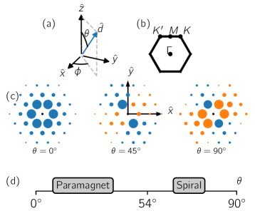
Figure 1: (Color online) Dipolar Heisenberg model on the triangular lattice in the $xy$ plane. (a) The exchange $J_{ij}$ depends on the dipole orientation $\hat{d}$, with polar angle $\theta$ and azimuthal angle $\phi$. (b) High symmetry points within the Brillouin zone. (c) The competing exchange couplings $J_{ij}$ (site $i$ is at the origin) for $\phi=30^{\circ}$ and $\theta=0^{\circ}$, $45^{\circ}$ and $90^{\circ}$ respectively. The size of the circle indicates the magnitude of $J_{ij}$, with positive (negative) $J_{ij}$ shown in blue (orange). (d) The zero temperature phase diagram at $\phi=30^{\circ}$ includes a wide quantum paramagnetic phase, $\theta\in[0,54^{\circ})$, and a spiral phase.

Pseudo-fermion FRG. The key to find the phase diagram of the quantum dipolar Heisenberg model is an accurate, unbiased many-body technique that can treat the spiral order, long-range interactions, and large lattices. Functional renormalization group (FRG) is well suited for this purpose. It starts with the bare interaction, and systematically integrates out the high energy, short wave length fluctuations to track the flow of the effective action functional. Under the flow toward lower energy and longer wave length, the leading many-body instability emerges as the dominant divergence. We follow the pseudo-fermion FRG (pf-FRG) put forward by Reuther and Wölfle, which has been extensively benchmarked against other methods and applied to frustrated spin models Reuther and Wölfle (2010); Reuther and Thomale (2011); Reuther et al. (2011, 2014); Suttner et al. (2014); Buessen and Trebst (2016); Iqbal et al. (2015, 2016). The spin model Eq. (1) is first rewritten in a fermionic representation via $\mathbf{S}_{i}=\frac{1}{2}\mathbf{\sigma}_{\alpha\beta}\psi^{\dagger}_{\alpha i}\psi_{\beta i}$ where $\psi$’s are fermionic field operators. The resulting interacting fermion problem is then solved using the well-established fermionic FRG developed for strongly correlated electrons Metzner et al. (2012); Kopietz et al. (2010); Bhongale et al. (2012); Keleş and Zhao (2016). Specifically, vertex expansion up to one loop order yields the flow equations for the fermion self energy $\Sigma$ and the effective interaction vertex $\Gamma$ as functions of the sliding RG scale $\Lambda$,

$$\partial_{\Lambda}\Sigma(\omega_{1}) =-\sum_{2}\Gamma_{1,2;1,2}S(\omega_{2}),$$ (3)

$$\partial_{\Lambda}\Gamma_{1^{\prime},2^{\prime};1,2} =\sum_{3,4}\Pi(\omega_{3},\omega_{4})\biggr{[}\frac{1}{2}\Gamma_{1^{\prime},2^{\prime};3,4}\Gamma_{3,4;1,2}$$

$$-\Gamma_{1^{\prime},4;1,3}\Gamma_{3,2^{\prime};4,2}+\Gamma_{2^{\prime},4;1,3}\Gamma_{3,1^{\prime};4,2}\biggr{]}.$$ (4)

Hereafter the $\Lambda$ dependence of $\Sigma$, $\Gamma$, $G$, $S$ etc. is omitted for brevity, and we use the shorthand notation $\Gamma_{1^{\prime},2^{\prime};1,2}\equiv\Gamma(i_{1},\alpha_{1},\omega_{1},i_{2},\alpha_{2},\omega_{2};i_{1}^{\prime},\alpha_{1}^{\prime},\omega_{1}^{\prime},i_{2}^{\prime},\alpha_{2}^{\prime},\omega_{2}^{\prime})$ with site index $i$, spin $\alpha$ and frequency $\omega$. The sum denotes integration over $\omega$ as well as summation over lattice sites and spin. The scale-dependent propagators are defined by

$$G(\omega)=\frac{\Theta(|\omega|-\Lambda)}{i\omega+\Sigma(\omega)},\quad S(\omega)=\frac{\delta(|\omega|-\Lambda)}{i\omega+\Sigma(\omega)}.\quad$$ (5)

Note that the bare fermion propagator only has frequency dependence, $G^{(0)}(\omega)=1/i\omega$ . Eq. (4) includes the particle-particle, the particle-hole as well as the exchange channel as shown by the following diagrams:

$$\leavevmode\hbox to71.85pt{\vbox to34.97pt{\text{[drawing]}}}+\leavevmode\hbox to72.62pt{\vbox to34.97pt{\text{[drawing]}}}+\leavevmode\hbox to72.62pt{\vbox to34.97pt{\text{[drawing]}}} 1 2 1^{\prime} 2^{\prime} 3 4 1 1^{\prime} 2 2^{\prime} 3 4 1 2^{\prime} 2 1^{\prime} 3 4 1 2 1^{\prime} 2^{\prime} 3 4 1 1^{\prime} 2 2^{\prime} 3 4 1 2^{\prime} 2 1^{\prime} 3 4$$

We adopt an improved truncation scheme beyond one loop Katanin (2004) where the bubble $\Pi$ is given by the full derivative

$$\Pi(\omega_{3},\omega_{4})=-\frac{d}{d\Lambda}\left[G(\omega_{3})G(\omega_{4})\right].$$ (6)

The first order nonlinear integro-differential equations in Eq. (3) and (4) are supplemented by the following initial conditions at the ultraviolet scale $\Lambda_{\mathrm{UV}}\rightarrow\infty$,

$$\Sigma(\omega)|_{\Lambda_{\mathrm{UV}}} =0,$$ (7)

$$\Gamma_{1,2;1^{\prime},2^{\prime}}|_{\Lambda_{\mathrm{UV}}} =\frac{1}{4}\sigma^{\mu}_{\alpha_{1}\alpha_{1}^{\prime}}\sigma^{\mu}_{\alpha_{2}\alpha_{2}^{\prime}}J_{i_{1},i_{2}}\delta_{i_{1}i_{1}^{\prime}}\delta_{i_{2}i_{2}^{\prime}}-(1^{\prime}\leftrightarrow 2^{\prime}).$$

We numerically solve the coupled flow equations Eq. (3)-(4) together with the initial condition Eq. (7) and the dipolar exchange Eq. (2) using the fourth order Runge-Kutta, for a logarithmic frequency grid of $N_{\omega}$ frequencies, by taking $N_{\Lambda}$ RG steps from bare scale $\Lambda_{\mathrm{UV}}$ down to zero. We keep all couplings $\Gamma$ within an $N_{L}\times N_{L}$ parallelogram on the triangular lattice sup . The computational cost scales with $N_{\Lambda}\cdot N_{L}^{2}\cdot N_{\omega}^{4}$. We perform simulations up to $N_{L}=13$, $N_{\omega}=64$, and $N_{\Lambda}=4N_{\omega}$, i.e. four RG steps between two neighboring frequency points. Following the efficient spin and frequency parametrization scheme of Ref. Reuther and Wölfle, 2010, and exploiting the reflection symmetry of $H$, we still end up with over 22 million coupling constants ($\Gamma$s). To make the calculation tractable, the FRG code is designed to run parallel on thousands of graphic processing units. We have benchmarked it and found good agreement with known FRG results on the square Reuther and Wölfle (2010) and triangular Iqbal et al. (2016) lattice $J_{1}$-$J_{2}$ model.

From $\Gamma$ and $\Sigma$, we compute the static spin-spin correlation functions in real space and then Fourier transform to obtain the spin susceptibility $\chi(\mathbf{p})$ Reuther and Wölfle (2010). Let $\chi_{\mathrm{max}}$ be the maximum value of $\chi$ reached at wave vector $\mathbf{p}=\mathbf{p}_{\mathrm{max}}$ within the Brillouin zone shown in Fig. 1(b). Together $\chi(\mathbf{p})$ and $\mathbf{p}_{\mathrm{max}}$ offer clues about the onset or lack of long-range order under the FRG flow. Typically $\chi_{\mathrm{max}}$ displays Curie-Weiss behavior for $\Lambda\gg 1$ until the build-up of quantum correlations starts to kick in around $\Lambda\sim 1$. An instability towards long range order is signaled by the divergence of $\chi_{\mathrm{max}}$ at some critical scale $\Lambda_{c}<1$. The finite cluster size and the truncation and discretization regularize the divergence, and replace it with unstable, irregular and oscillatory flow below $\Lambda_{c}$. Despite this, the breakdown of the smooth flow is unmistakable, and the type of incipient order can be inferred from the location of $\mathbf{p}_{\mathrm{max}}$. It may also happen that the flow of $\chi$ remains stable and smooth down to the lowest RG scale $\Lambda\rightarrow 0$. Then the system settles into a paramagnetic phase.

To orient the full FRG solution and compare with the classical results, we first carry out static FRG, i.e. solving the flow equations by ignoring all $\omega$ dependences sup ; Baez and Reuther (2017). This approximation was shown to be consistent with random phase approximation and Luttinger-Tisza method Baez and Reuther (2017). From the flow of $\Gamma$, we extract a “critical scale” $\Lambda_{s}$, at which the maximum value of $\Gamma$ reaches a large cutoff value (diverges). Thus $\Lambda_{s}$ serves as a rough estimation of the critical temperature for the long-range order. Fig. 2 shows the resulting $\Lambda_{s}$ in false color with contour lines. Here we find good agreement with the classical analysis. The $120^{\circ}$ order, where $\chi$ shows maxima at the corners of the Brillouin zone, lies at small $\theta$. For increasing $\theta$, peaks at $K$ and $K^{\prime}$ come together and merge at the $M$ point, indicating the stripe phase. For even larger $\theta$, the peak at $M$ moves towards the $\Gamma$ point, signaling the spiral order. Fig. 2 also shows that the spiral phase has the largest $\Lambda_{s}$ (in green) whereas $\Lambda_{s}$ is significantly suppressed (in dark blue) in the region around $\theta\sim 15^{\circ}$ and near the phase boundaries. These dark areas are where spin liquid is suspected to reside.

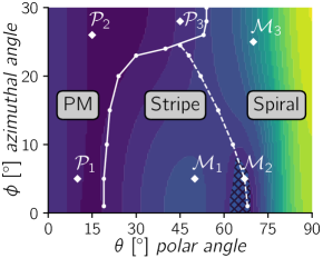
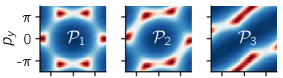
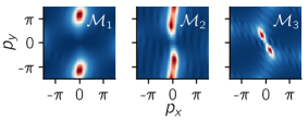
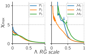
Figure 2: (Color online) Zero temperature phase diagram of the dipolar Heisenberg model on triangular lattice as a function of the dipole tilting angle ($\theta$, $\phi$) showing the quantum paramagnetic (PM), stripe and spiral phases. Solid and dashed white lines are the phase boundaries (see main text). Color contours shows estimated critical temperature $\Lambda_{s}$ from static FRG. Spin susceptibility profiles $\chi(\mathbf{p})$ at scale $\Lambda<0.5$ are shown in the middle panels for representative points marked with $\mathcal{P}_{1}$, $\mathcal{M}_{1}$ etc.. The flows of peak susceptibility $\chi_{\mathrm{max}}$ are shown in the bottom panels. For $\mathcal{M}_{1}$ and $\mathcal{M}_{3}$, the flow becomes unstable below some RG scale indicated by the arrows.

Phase diagram from pf-FRG. Solving the flow equations with full frequency dependence along multiple cuts on the $(\theta,\phi)$ plane and examining the flow of $\chi_{\mathrm{max}}$ and the profile of $\chi(\mathbf{p})$ in momentum space, we arrive at the zero temperature phase diagram of the dipolar Heisenberg model on triangular lattice shown in Fig. 2. The solid line and the dashed line mark the phase boundary between three major phases: the stripe, the spiral, and the quantum paramagnetic (PM) phase. The most striking result from pf-FRG is the abundance of the PM phase. A large portion of the classical spiral, including the $120^{\circ}$ order, completely melts due to strong quantum fluctuations and gives way to quantum paramagnet. Compared to the $J_{1}$-$J_{2}$ Heisenberg model which shows a narrow region of spin liquid between the $120^{\circ}$ and stripe order Zhu and White (2015); Hu et al. (2015), here the long-range dipolar exchanges suppress the $120^{\circ}$ order to favor a disordered state. Our result agrees with earlier DMRG study of dipolar Heisenberg model for $\phi=0$ with truncated interactions Yao et al. (2018). Both predict a spin disordered phase for $\theta<\theta_{c}$, with $\theta_{c}\sim 19^{\circ}$ from pf-FRG and $\theta_{c}\sim 10^{\circ}$ from DMRG. Our new insight is that the PM phase becomes much broader, $\theta_{c}\sim 54^{\circ}$, if we tune $\phi$ to $30^{\circ}$ to suppress the stripe phase.

Now we discuss the pf-FRG results for a few representative points on the phase diagram. Let us start with the point $\mathcal{P}_{1}$ in Fig. 2, $\theta=10^{\circ}$, $\phi=5^{\circ}$. The spin susceptibility profile $\chi(\mathbf{p})$ at $\Lambda\approx 0.2$ is shown in the middle panel. It peaks at $K$ and $K^{\prime}$, indicating the $120^{\circ}$ correlations. There is however no long-range order. We find instead a remarkably smooth flow of $\chi_{\mathrm{max}}$ down to $\Lambda\rightarrow 0$ without any sign of instability in the bottom panel of Fig. 2. Note that small fluctuations at small $\Lambda$ are artifacts due to the frequency discretization and they diminish with finer grid. Similar PM behaviors are observed for point $\mathcal{P}_{2}$ and $\mathcal{P}_{3}$ at larger values of $\phi$, with the $\chi(\mathbf{p})$ profile titled accordingly. These are our most significant findings.

Moving from point $\mathcal{P}_{1}$ towards $\mathcal{M}_{1}$, the peaks at $K$ and $K^{\prime}$ first become flatter and eventually coalesce at $\theta=17^{\circ}$. Here $\chi_{\mathrm{max}}$ shows a massive degeneracy in $\mathbf{p}$-space: it peaks along the entire $K$-$K^{\prime}$ line. Beyond this point, the flow of $\chi_{\mathrm{max}}$ shows increasing jumps at small $\Lambda$, and a kink (or turning point, indicated by the small arrow) is developed for $\theta>19^{\circ}$. At the point $\mathcal{M}_{1}$, $\chi(\mathbf{p})$ is sharply peaked at $M$, and the flow becomes unstable at small $\Lambda$, clearly indicating the stripe phase. Increasing $\theta$ further beyond the point $\mathcal{M}_{2}$, $\chi(\mathbf{p})$ develops a peak at a location between the $M$ and $\Gamma$ point. Similar result is obtained for other values of $\phi$, such as the $\mathcal{M}_{3}$ point in Fig. 2. Here, the sharp peak of $\chi(\mathbf{p})$ as well as the unstable flow unambiguously identify the spiral order.

To locate the phase boundaries in a systematic manner, we introduce an empirical measure to quantify and detect the breakdown of smooth FRG flow. For a given dipolar tilting, we compute $f(\theta,\phi)=\sum_{\Lambda}(\chi_{\mathrm{max}}\big{|}_{\Lambda}-\chi_{\mathrm{max}}\big{|}_{\Lambda-d\Lambda})^{2}$, i.e. the “sum of unphysical jumps” during the flow. The value of $f$ is very small in the paramagnetic phase because of smooth continuous flow, and very large for ordered phases because their unstable flow sup . By comparing to DMRG, we know that at $\theta=0$, independent of $\phi$, the system is deep inside the PM phase. Thus, it provides a standard measure $f_{0}=f(\theta=0,\phi=0)$. If $f(\theta,\phi)\leq f_{0}$, the low energy flow is equally smooth or even smoother than that at $\theta=0$, we then conclude the system flows to a disordered, paramagnetic phase. The resulting boundary of the PM phase is shown by the solid white line bending to the right in Fig. 2. The transition from PM to stripe is marked by a rapid increase in $f/f_{0}$. In contrast, the transition from stripe to spiral is signaled by smoothening of the flow and thus suppression of $f$ (see the flow for $\mathcal{M}_{2}$ in Fig. 2). We identify the stripe-spiral boundary as where $f$ develops a local minimum along the horizontal cuts on the $(\theta,\phi)$ plane. It is shown by the white dashed line bending to the left in Fig. 2. This line is also where the peaks in $\chi(\mathbf{p})$ become smeared and the location of $\mathbf{p}_{\mathrm{max}}$ begins to change character. In the hatched region around $\mathcal{M}_{2}$ in Fig. 2, the flow is much smoother than $\mathcal{M}_{1}$ and $\mathcal{M}_{3}$ at small $\Lambda$. It is analogous to $\mathcal{P}_{1}$ but $\chi_{\mathrm{max}}$ reaches a much bigger value at $\Lambda=0$. Therefore, this small region is likely a second PM phase, but on the verge of being ordered.

To summarize, our numerical FRG calculation reveals a quantum paramagnetic phase occupying a large portion of the phase diagram of the dipolar Heisenberg model. FRG enables us to reach large cutoff distances for an accurate description of the dipolar exchange and the spiral order. It describes quantum fluctuations beyond the spin-wave or Schwinger-boson theory. The widespread lack of divergence in $\chi$ is unexpected. In hindsight, three factors conspire to suppress long-range order. First is the lattice geometric frustration. Second, the stripe order is completely suppressed for dipole titling $\phi=30^{\circ}$ due to symmetry, such that the paramagnetic phase extends to as far as $\theta=54^{\circ}$. Third is the competition of $J_{ij}$, i.e. exchange frustration, stemming from the long-range dipolar exchange (see Fig. 1). Even in the $J_{1}$-$J_{2}$ model, finite $J_{2}$ enhances paramagnetic behavior Hu et al. (2015); Zhu and White (2015); Saadatmand and McCulloch (2017). Longer range exchanges lead to very flat classical energy landscape, with distinct orders close in energy. These weak classical orders are melted by quantum fluctuations to form a quantum paramagnet.

Our results suggest that experiments on ultracold quantum gases of polar molecules with electric dipole moments or atoms with large magnetic dipole moments are promising systems to explore frustrated magnetism and search for spin liquids Yan et al. (2013); de Paz et al. (2013). There are two limitations to the current pf-FRG method. First, the flow equation is restricted to one-loop diagrams. An improvement is to include two-loop terms as achieved recently in Ref. Rueck and Reuther (2017). Second, current pf-FRG implementation cannot directly characterize the spin liquid states. Future work is needed to elucidate the nature of the predicted spin liquid states in various spin $1/2$ models on the triangular lattice Essin and Hermele (2013); Lu (2016), which remains an outstanding open problem.

Supplementary Materials for “Absence of long-range order in a triangular spin system with dipolar interactions”

Ahmet Keleş and Erhai Zhao

I Classical Phase Diagram

To find the classical ground states of dipolar Heisenberg model, we substitute the operator $\mathbf{S}$ with classical vector $S_{i}=S(\cos\mathbf{q}\cdot\mathbf{r}_{i},\sin\mathbf{q}\cdot\mathbf{r}_{i},0)$ in the Hamiltonian $H=\sum_{ij}J_{ij}\mathbf{S}_{i}\cdot\mathbf{S}_{j}$ with dipolar coupling $J_{ij}$ and obtain the classical energy

$$E_{\mathrm{cl}}(\mathbf{q})=S^{2}\sum_{ij}J_{ij}\cos(\mathbf{q}\cdot\mathbf{r}_{i}-\mathbf{q}\cdot\mathbf{r}_{j}).$$ (S1)

We minimize $E_{\mathrm{cl}}$ with respect to $\mathbf{q}=(q_{x},q_{y})$ to find the ordering wave vector $\mathbf{q}_{min}$. As an example, we plot the energy landscapes $E_{\mathrm{cl}}(\mathbf{q})$ and the corresponding spin configurations in real space for three representative angles in Fig. S1. Here, we have chosen a 40-by-40 lattice grid and performed the summation numerically for each value of $\mathbf{q}$ in the Brillouin zone. By performing this analysis for each point in the parameter space of dipolar tilting $(\theta,\phi)$, the phase diagram of the system can be found as shown in Fig. S1.

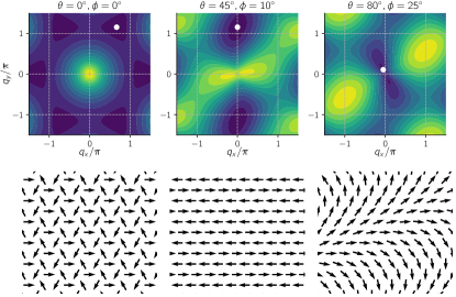
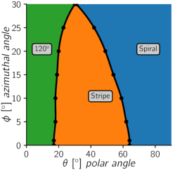
Figure S1: Left: the top row shows classical energy landscapes $E_{\mathrm{cl}}(\mathbf{q})$ as a function of $q_{x}$ and $q_{y}$ for three different dipolar tilting angles. Dark (blue) regions are energy minima whereas bright (yellow) regions are energy maxima. The wavevector minimizing the energy is indicated with a white dot in each figure. The bottom row shows the ordering (spin configuration) in real space for the minimum energy wavevector $\mathbf{q}=\mathbf{q}_{min}$. Right: the phase diagram obtained from classical analysis showing three phases.

From the locations of the minima in the energy landscape, one can see the $120^{\circ}$ order for small tilting with ordering vector $\mathbf{q}_{min}=2\pi(1/3,1/\sqrt{3})$, the stripe order for intermediate tilting with $\mathbf{q}_{min}=2\pi(0,1/\sqrt{3})$, and finally the spiral order with wavevectors that are generally incommensurate with the lattice spacing and change continuously within the Brillouin zone with dipolar angles. Fig. S1 is obtained by scanning the $(\theta,\phi)$ plane along a few horizontal cuts and finding the phase boundaries along these cuts.

II Frequency independent Functional Renormalization

When frequency dependence of the vertex is ignored, the self energy term in the flow equations vanishes and the following spin parametrization can used

$$\Gamma_{1^{\prime},2^{\prime};1,2}=\Gamma_{s}(i_{1},i_{2})\delta_{i_{1}^{\prime}i_{1}}\delta_{i_{2}^{\prime}i_{2}}\sigma_{\alpha_{1}^{\prime}\alpha_{1}}\sigma_{\alpha_{2}^{\prime}\alpha_{2}}-(1^{\prime}\leftrightarrow 2^{\prime}),$$ (S2)

which obeys the following simplified flow equation

$$\frac{d}{d\Lambda}\Gamma_{s}(i_{1},i_{2})=\frac{2}{\pi}\frac{1}{\Lambda^{2}}\biggr{[}-2\Gamma_{s}(i_{1},i_{2})\Gamma_{s}(i_{1},i_{2})+\Gamma_{s}(i_{1},i_{2})\Gamma_{s}(i_{1},i_{1})+\sum_{j}\Gamma_{s}(i_{1},j)\Gamma_{s}(j,i_{2})\biggr{]}.$$ (S3)

Note that a parametrization in the density channel is also allowed by symmetry in the form $\delta_{\alpha_{1}^{\prime}\alpha_{1}}\delta_{\alpha_{2}^{\prime}\alpha_{2}}$, however such a term vanishes under frequency independent renormalization flow as demonstrated in Ref. Reuther and Wölfle (2010) and therefore can be neglected (we will implement parametrization in the density channel in the next section). The factor in front of the right hand side of Eq. (S3) comes from the remaining frequency dependence of Green function bubble and the integral of this term is calculated as

$$\frac{1}{2\pi}\int d\omega 2\Pi(\omega,\omega) =\frac{1}{\pi}\int d\omega\frac{1}{\omega^{2}}\delta(|\omega-\Lambda|)\Theta(|\omega|-\Lambda)$$

$$=\frac{1}{\pi}\left[\frac{1}{2}\frac{1}{\Lambda^{2}}+\frac{1}{2}\frac{1}{(-\Lambda)^{2}}\right]=\frac{1}{\pi}\frac{1}{\Lambda^{2}}.$$ (S4)

The first order coupled differential equations are solved numerically starting from the initial condition at the bare (ultraviolet) scale $\Lambda_{UV}$

$$\Gamma_{s}(i_{1},i_{2})\biggr{|}_{\Lambda=\Lambda_{UV}}=\frac{1}{4}J_{ij}$$ (S5)

down to the infrared scale $\Lambda_{0}\ll 1$. From the vertex, the static spin susceptibility can be calculated as

$$\chi(i_{1},i_{2})\equiv\langle S^{z}_{i_{1}}S^{z}_{i_{2}}\rangle=\frac{1}{2\pi\Lambda}\delta_{i_{0}i_{2}}-\frac{1}{\pi^{2}\Lambda^{2}}\Gamma_{s}(i_{1},i_{2}).$$ (S6)

From translational invariance, the vertex $\Gamma_{s}$ only depends on $i_{1}-i_{2}$. To monitor the flow, we Fourier transform the susceptibility and inspect its momentum space profile. Since the only energy scale in the problem is the exchange energy $J_{0}$ which is taken to be the unit of energy, we set up a renormalization grid for $\Lambda$ starting from two orders of magnitude smaller than this scale $\Lambda_{0}\propto 10^{-2}$ up to two orders of magnitude larger than the exchange scale $\Lambda_{UV}\propto 10^{2}$ with logarithmically spaced mesh. We have checked that further increasing this interval (e.g. increasing $\Lambda_{UV}$) does not change the FRG flow noticeably.

The phase boundary can be located by inspecting the susceptibility profile $\chi(\mathbf{p})$ for each parameter to determine its peak location. Since the sharp peaks turn to flat ridges near the phase boundaries, it is much more convenient to pinpoint the phase boundary by monitoring the degeneracy of the susceptibility profile. For example, as we move along a horizontal cut going from the $120^{\circ}$ phase to the stripe phase, the maxima at $K$ and $K^{\prime}$ points gets elongated and eventually merge to give the shape of an extended ridge along the $K-K^{\prime}$ line at the phase boundary. Once we enter the stripe phase, the maxima at $M$ point dominates to lift the degeneracy along the $K-K^{\prime}$ line. To determine the degeneracy, we divide the momentum space into $N_{bins}$ bins and count $N_{peak}$, the number of bins within which $\chi(\mathbf{p})$ reaches at least 90 percent of its maximum value. Then the degeneracy is assigned as $N_{peak}/N_{bins}$. The phase diagram resulting from this analysis is shown in Fig. S2. It is very similar to the classical diagram Fig. S1. Note the static FRG takes into quantum fluctuations not considered in the classical analysis. As a result, the $120^{\circ}$-stripe boundary is pushed slightly to the left, while the stripe-spiral boundary is shifted slightly to the right, each by about 2^∘. The agreement with the classical phase diagram serves as a sanity check for the back bone of our FRG calculation.

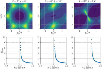
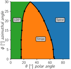
Figure S2: Right: phase diagram of the dipolar Heisenberg model on triangular lattice from static (frequency-independent) FRG calculation, in good agreement with classical analysis. Left: the susceptibility profiles for three selected points in the phase diagram and the corresponding renormalization flow of the susceptibility maximum. The divergence of spin susceptibility maximum indicates long-range order. Dark (blue) regions are susceptibility minima whereas bright (yellow) regions are susceptibility maxima.

III Details of Full Functional renormalization implementation

For numerical implementation of FRG flow equations with full frequency dependence, we use the following parametrization

$$\Gamma_{1^{\prime},2^{\prime},1,2}=\Gamma^{\mathrm{spin}}_{i_{1}i_{2}}(s,t,u)\sigma_{\alpha_{1}^{\prime}\alpha_{1}}\sigma_{\alpha_{2}^{\prime}\alpha_{2}}\delta_{i_{1}^{\prime}i_{1}}\delta_{i_{2}^{\prime}i_{2}}+\Gamma^{\mathrm{density}}_{i_{1}i_{2}}(s,t,u)\delta_{\alpha_{1}^{\prime}\alpha_{1}}\delta_{\alpha_{2}^{\prime}\alpha_{2}}\delta_{i_{1}^{\prime}i_{1}}\delta_{i_{2}^{\prime}i_{2}}-(1^{\prime}\leftrightarrow 2^{\prime})$$ (S7)

where $(1^{\prime}\leftrightarrow 2^{\prime})$ implements fermionic antisymmetry and frequency dependence is expressed in terms of Mandelstam variables $s=\omega_{1}+\omega_{2}=\omega_{1}^{\prime}+\omega_{2}^{\prime}$, $t=\omega_{1}-\omega_{1}^{\prime}$ $u=\omega_{1}-\omega_{2}^{\prime}$. In this parametrization, the first term is the spin-spin interaction parametrized by the well known $\sigma\cdot\sigma$ form, whereas the second term is the density-density interactions. Site dependence is parametrized by terms like $\delta_{i_{1}^{\prime}i_{1}}$ or $\delta_{i_{1}^{\prime}i_{2}}$ so that a $\psi^{\dagger}$ term is matched with $\psi$ term in the interaction vertex $\psi^{\dagger}\psi^{\dagger}\psi\psi$. This parametrization, along with site independent self energy and full Green function

$$G(i_{1}^{\prime},\omega_{1}^{\prime},\alpha_{1}^{\prime};i_{1},\omega_{1},\alpha_{1};)=\delta_{i_{1}^{\prime}i_{1}}\delta_{\omega_{1}^{\prime}\omega_{1}}\frac{1}{i\omega_{1}+\Sigma(\omega_{1})}$$ (S8)

ensures that the fermion hopping is forbidden and number of fermion per site is fixed at one. This has been discussed in detail in Ref. Reuther and Wölfle, 2010. It has been explicitly checked in Ref. Buessen et al., 2018 that the fermion number constraint is preserved exactly in pseudofermion FRG at zero temperature as implemented here.

Once $G$ and $\Gamma$ are obtained from the numerical renormalization flow, we calculate the static spin susceptibility using the following diagrammatic expression

$$\chi_{i_{1},i_{2}}=\int_{0}^{\infty}d\tau\langle TS_{i_{1}}(\tau)S_{i_{2}}(0)\rangle=\leavevmode\hbox to166.23pt{\vbox to27.33pt{\text{[drawing]}}} + +$$ (S9)

where “” is the representation for the Pauli matrix $\sigma$ for spin at site $i$, $S_{i}=1/2\sigma_{\alpha^{\prime}\alpha}\psi^{\dagger}_{\alpha^{\prime}i}\psi_{\alpha i}$.

III.1 A. Frequency Grid

We use the zero temperature formalism such that the Matsubara frequencies become continuous variables $\omega\in[-\infty,\infty]$ and frequency summations become infinite integration $\int_{-\infty}^{\infty}d\omega/2\pi$. Since the vertex contains three independent frequency variables (the fourth one is given by energy conservation), the computational cost increases quickly as the frequency resolution is increased. Changing frequency variables into Mandelstam form significantly reduces the cost due to symmetry of the vertex $s\rightarrow-s$, $t\rightarrow-t$, $u\rightarrow-u$ and self energy $\Sigma(-\omega)=-\Sigma(\omega)$ as shown in Ref. Reuther and Wölfle (2010) based on the structure of the flow equations. As a result, it is sufficient to restrict the frequency integrations to positive axis $\int_{0}^{\infty}d\omega$ based on this symmetry. For numerical implementation, one has to introduce minimum $\omega_{min}$ and maximum $\omega_{max}$ frequencies in the positive axis which can be considered as ultraviolet and infrared limits of the theory. In choosing these limits, we have to remember that the only energy scale is the dipolar exchange energy $J_{0}$ defined in Eq. 1 of main text which is taken to be the unit of energy in our theory, i.e. $J_{0}=1$. Thus, the conditions on the frequency limits are $w_{max}\gg 1$ and $\omega_{min}\ll 1$. In our simulations we take $\omega_{max}=100$ or $400$ and $\omega_{min}=0.01$ or $0.005$ and checked that the final results do not change.

The most important step in setting up the frequency grid is to decide the number of points between $\omega_{min}$ and $\omega_{max}$ and their spacing. Recall that the frequency dependence of the running couplings is weak at large frequencies due to the Green function bubbles in the flow equation. So we choose a logarithmically spaced frequency grid, with a spacing increasing with $\omega$, containing $N_{\omega}=48$ or $64$ points within the entire frequency range. We have check that the final results do not change with further increase in $N_{\omega}$ or when we switch to a grid with spacing given by a geometric series $\omega_{n}=\omega_{min}(\epsilon^{n}-1)/(\epsilon-1)$ with grid parameter $\epsilon$ determined by $\omega_{n=N_{\omega}}=\omega_{max}$. Once the frequency grid is set up, the RG grid is automatically determined which can be symbolically demonstrated as

We take four renormalization steps between each frequency grid and solve the flow equation using standard Runge-Kutta method. Due to discreteness of the frequencies, there may be small “oscillations” in the flow of $\chi$ as $\Lambda$ moves from one frequency grid point to the next (see for example, point $\mathcal{P}_{1}$ and $\mathcal{P}_{3}$ in Fig. S3). These small oscillations are natural for any numerical implementation and well controlled: they can be reduced by choosing a denser grid.

III.2 B. Truncation of Interaction Range

We emphasize that our calculation is not done for a finite lattice with open boundary conditions. We assume translational invariance such that the vertex $\Gamma^{\mathrm{spin}}_{i_{1}i_{2}}$ and $\Gamma^{\mathrm{density}}_{i_{1}i_{2}}$ only depend on the difference $\mathbf{r}_{i_{1}}-\mathbf{r}_{i_{2}}$ which can be visualized as a bond between site $i_{1}$ and site $i_{2}$. Note that each bond has three frequency variables. In practice, the computational cost increases rapidly with the number of bonds and the number of discrete frequencies. We choose a reference site $i_{1}$ at the origin, consider all bonds within the region of a $N_{L}$-by-$N_{L}$ parallelogram and discard bonds outside this region. (We have also tried a circular cutoff region with radius $N_{L}$. The results are essentially the same for sufficiently large $N_{L}$. The parallelogram is adopted because it is easy to implement on parallel computing platforms.) Formally, this corresponds to an infinite spin system with truncated effective interaction range. (In the pfFRG literature, this truncation in the interaction range is simply referred to as “the cluster size” for brevity. It is not to be confused with a finite lattice with open boundary conditions. There is no physical boundary in our implementation. In passing, we mention that periodic boundary conditions have recently been considered within pfFRG in an alternative implementation in Ref. Göttel et al. (2012).) It is critical to choose a sufficiently large $N_{L}$ while keeping the calculation feasible on modern GPU devices.

From the real space susceptibility data $\chi_{i_{1},i_{2}}\equiv\chi(\mathbf{r}_{i_{1}}-\mathbf{r}_{i_{2}})$, we take the Fourier transform as

$$\chi(\mathbf{p})=\sum_{i_{1}-i_{2}}\chi_{i_{1},i_{2}}e^{i\mathbf{p}\cdot(\mathbf{r}_{i_{1}}-\mathbf{r}_{i_{2}})}.$$ (S10)

Here, the number of points $\mathbf{p}$ in the Brillouin zone can be taken as arbitrarily large, since an infinite lattice is assumed. By inspecting $\chi(\mathbf{p})$, we determine the leading ordering tendency from the maximum susceptibility $\chi_{\mathrm{max}}$ and monitor its RG flow. To understand the susceptibility flows, one can view heuristically the renormalization scale $\Lambda$ as the temperature of the system. Probing collective phenomena at lower energies by reducing the sliding RG scale corresponds to reducing the temperature of the system. At low temperatures, the system either enters into a magnetically ordered phase or stays paramagnetic down to the lowest numerical scales. If a magnetic order develops, the correlations functions such as the spin susceptibility would show divergence at some critical temperature. At this point, the correlation length becomes infinite indicating long range order in the thermodynamic limit. However, since we have to truncate the correlations due to finite computational resources, such divergences will be regulated. Therefore, instead of a simple divergence commonly encountered in single channel RG, the growth of $\chi_{\mathrm{max}}$ beyond the critical scale $\Lambda_{c}$ will eventually be replaced by unstable flows as shown in Fig. S3 for point $M_{1}$ and $M_{3}$. This is the price we have to pay for retaining all channels on equal footing and flowing the entire $\Gamma$ instead of just a few running couplings. In practice, the breakdown of smooth flow beyond the critical scale is actually a blessing. It serves as a telling sign of the many-body instability toward the development of long range order. In contrast, if the FRG flow smoothly reaches the lowest infrared scale without any disturbance (see point $\mathcal{P}_{1}$ and $\mathcal{P}_{3}$ in Fig. S3), there is no indication for long range order and the ground state is a quantum paramagnet.

We have systematically investigated the effect of varying $N_{L}$ on the flow and phase boundary. Some examples are shown in Fig. S3 for a few different truncations ($N_{L}=7$, $13$ and $19$).

Paramagnetic phase – We observe that the RG flows for parameters within the quantum paramagnetic phase, such as point $\mathcal{P}_{1}$ and $\mathcal{P}_{3}$, remain smooth and finite. Susceptibilities stay almost unchanged when we double or triple $N_{L}$. Such $N_{L}$-independence points to a quantum paramagnetic phase in the thermodynamic limit, and is consistent with the conjecture that it is a spin liquid with short range correlations.

Magnetic phases – On the other hand, for the stripe ($\mathcal{M}_{1}$ point) and spiral phase ($\mathcal{M}_{3}$ point), the onset of the long range order can be easily identified from the RG flows in Fig. S3. Here the susceptibility shows a divergence tendency until a critical scale $\Lambda_{c}$ which is indicated roughly by the black arrows. For these two points, the divergence becomes stronger and the value of $\Lambda_{c}$ converges as $N_{L}$ is increased. Thus, the instability toward long range order is unequivocal. Below the critical scale $\Lambda<\Lambda_{c}$, the RG flows break down and show unphysical, discontinuous jumps depending on $N_{L}$, in sharp contrast to the continuous flows for point $\mathcal{P}_{1}$ and $\mathcal{P}_{3}$.

The spiral phase presents a challenge for FRG calculations. Ideally, a very large $N_{L}$ is preferred because the ordering wave vector $\mathbf{p}_{\mathrm{max}}$ may, in principle, depend on the details of the bare and effective interactions at longer distances beyond the cutoff $N_{L}$. This turns out not to be the case. We have checked that $\mathbf{p}_{\mathrm{max}}$ is not very sensitive to $N_{L}$ provided it is large enough (e.g. $N_{L}=13$). To get an accurate estimation of $\Lambda_{c}$ and the critical temperature for the spiral phase, which is not our main goal here, one has to carefully track the dependence of the flows as $N_{L}$ is increased, preferably to very large $N_{L}$, because the convergence of the flow is slower compared to the stripe phase. In summary, we emphasize that whether or not the systems flows into a long range ordered phase, as reflected by the breakdown of the smooth flow, does not depend in the choice of truncation $N_{L}$ (see Fig. S3). The identification of the spiral and stripe phase is thus unambiguous.

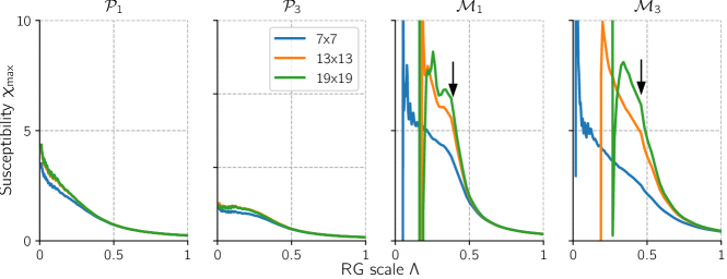
Figure S3: Renormalization flows of the susceptibility maxima $\chi_{\mathrm{max}}$ toward paramagnetic phases ($\mathcal{P}_{1}$, $\mathcal{P}_{3}$) and magnetic phases ($\mathcal{M}_{1}$, $\mathcal{M}_{3}$) for different truncations of interaction range $N_{L}=7,13$ and $19$. The black arrow indicates the critical scale $\Lambda_{c}$.

III.3 C. Estimation of the Phase Boundaries

Here we present additional details about the $f$ function introduced to estimate the phase boundary between the paramagnetic and magnetic phases,

$$f(\theta,\phi)=\sum_{\Lambda}(\chi_{\mathrm{max}}\big{|}_{\Lambda}-\chi_{\mathrm{max}}\big{|}_{\Lambda-d\Lambda})^{2}.$$ (S11)

By comparing the flows in Fig. S3, one can see that the value of $f$ is very small in the paramagnetic phase because of the smooth continuous flow, and very large for ordered phases because the unphysical discontinuous jumps below $\Lambda_{c}$. The value of $f$ changes dramatically as the phase boundary is crossed.

As an example, the left panel of Fig. S4 shows the values of $f$ along a cut for small azimuthal angle $\phi=1^{\circ}$ and $\theta$ from $0^{\circ}$ to $90^{\circ}$. Details of the susceptibility flow for selected points along this cut is shown in the top row of Fig. S5. The smooth, continuous flow at $\theta=0$ indicates a paramagnetic phase. This is consistent with the recent DMRG study that claims the ground state at this point is a spin liquid Yao et al. (2018). As $\theta$ is increased, $f$ stays flat before dipping slightly around $\theta=16^{\circ}$ and then starts increasing slowly afterwards. At $\theta=19^{\circ}$, $f$ reaches the same value at $\theta=0^{\circ}$ and we mark this point as the phase boundary (the phases are indicated by different color fillings in Fig. S4). Note that this is a conservative estimation, because a sharp increase of $f$ occurs later. So the paramagnetic phase may actually persist to larger values of $\theta$. In the stripe phase, $f$ is very large. Around $\theta=68^{\circ}$, $f$ shows a local minimum. This point is identified as the boundary between the stripe and spiral phase, and it is consistent with the change in the profile of $\chi_{\mathrm{max}}(\mathbf{p})$.

The right panel of Fig. S4 shows the value of $f$ for azimuthal angle $\phi=30^{\circ}$. The detailed flows of selected points are shown at the bottom row of Fig. S5. Here the paramagnetic phase persists to much larger $\theta$ angles. The same criterion for $f$ gives the phase boundary at $\theta_{c}=54^{\circ}$. The situation here differs from the small $\phi$ case. The stripe phase is completely suppressed and the paramagnetic phase directly transitions to the spiral phase.

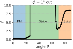
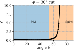
Figure S4: The value of $f$ along two distinct horizontal cuts of the phase diagram, $\phi=1^{\circ}$ (left) and $\phi=30$ (right).

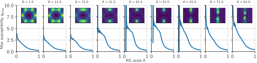
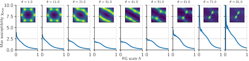
Figure S5: Details of the susceptibility flow for $\phi=1^{\circ}$ (top row) and $\phi=30^{\circ}$ (bottom row). The values of $\theta$ are shown in the title of each subplot. Insets show the susceptibility profiles in the Brillouin zone.