Utilizing Semantic Visual Landmarks for Precise Vehicle Navigation

Abstract

This paper presents a new approach for integrating semantic information for vision-based vehicle navigation. Although vision-based vehicle navigation systems using pre-mapped visual landmarks are capable of achieving submeter level accuracy in large-scale urban environment, a typical error source in this type of systems comes from the presence of visual landmarks or features from temporal objects in the environment, such as cars and pedestrians. We propose a gated factor graph framework to use semantic information associated with visual features to make decisions on outlier/ inlier computation from three perspectives: the feature tracking process, the geo-referenced map building process, and the navigation system using pre-mapped landmarks. The class category that the visual feature belongs to is extracted from a pre-trained deep learning network trained for semantic segmentation. The feasibility and generality of our approach is demonstrated by our implementations on top of two vision-based navigation systems. Experimental evaluations validate that the injection of semantic information associated with visual landmarks using our approach achieves substantial improvements in accuracy on GPS-denied navigation solutions for large-scale urban scenarios.

1 Introduction

Vehicle navigation using a pre-built map of visual landmarks has received lots of attention in recent years for future driver assistance systems or autonomous driving applications [1], which require sub-meter or centimeter level accuracy for situations such as obstacle avoidance or predictive emergency braking. The map of the environment is constructed and geo-referenced beforehand, and is used for global positioning during future navigation by matching new feature observations from on-board perception sensors to this map. Due to the low cost and small size of camera sensors, this approach is more appealing than traditional solutions using costly and bulky sensors such as differential GPS or laser scanners [2].

Using visual information from permanent structures rather than temporal objects ought to improve the mapping quality and navigation accuracy for these vision-based navigation systems. With new advances in deep learning, previously hard computer vision problems such as object recognition and scene classification can be solved with high accuracy. The availability of these trained models is able to make the use of vison-based navigation algorithms easier. For example, Figure 1 shows the result of using an off-the-shelf video segmentation tool to classify object categories from a street scene. As can be seen from the figure, even pre-trained networks achieve high accuracy and can help the navigation problem.

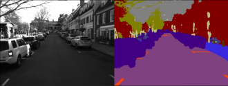
Figure 1: Output of a pre-trained Semantic Segmentation Network [3] used on one of our datasets. The figure above shows a use case for where semantic information is useful in mapping. Features from the parked vehicles can be considered to be temporal and should not be maintained in a long term map.

A recent survey on Simultaneous Localization and Mapping (SLAM) [4] shows the frontiers that have been explored in adding semantic information to the mapping process. They discuss the use of semantic information in mapping, and present arguments for both why semantic information aids SLAM and vice versa. These works have used different approaches to map the environment with different representations for semantic information in the environment. For instance, Choudhary et al [5] map indoor environments at the level of objects. Other works map the environment at the level of planes. These works highlight the importance of semantic mapping, which allows humans to localize themselves because they are able to associate geometric features with semantic categories.

However, the map maintained in these systems only preserves high-level objects/ planes or other semantic entities. These techniques are typically used in the domain of mobile robots that operate indoors. They are interested in maintaining representations of objects or locations of obstacles (such as walls) that the robot can maneuver, and are not directly applicable to the autonomous vehicle navigation problem we try to solve. In our application, it is important to maintain both high-level semantic information and low-level visual features associated with landmarks mapped in the environment. In addition, these works use complex algorithms to perform image/video segmentation to derive semantic information for the localization and mapping process. With recent advances in deep learning, segmentation tasks can be replaced with simpler and off the shelf tools.

In this paper, we present a simple and effective approach for integrating semantic information extracted from a pre-trained deep learning network for vehicle navigation. We propose a new framework which utilizes the semantic information associated with each imaged feature to make a decision on whether to use this feature point in the system. This feature selection mechanism based on semantic information can be performed for both the feature tracking process in the real-time navigation system and the map building process beforehand. For example, as shown in Figure 1, imaged features from the parked vehicles can be considered to be temporal and should not be maintained in the map during the map building process.

Our framework is designed to be applied to any vision-based SLAM systems for vehicle navigation. To demonstrate the feasibility and generality of our approach, we apply our framework on two state-of-the-art visual-based navigation systems [6, 7]. The popular ORB-SLAM2 system [7] uses only cameras as the input sensor, and cannot build geo-referenced maps beforehand. Without the use of pre-built maps, we show our approach improves its navigation accuracy by polishing its feature tracking process.

We also utilize the system from [6], which efficiently fuses pre-mapped visual landmarks as individual point measurements to achieve sub-meter overall global navigation accuracy in large-scale urban environments. This system constructs the visual map beforehand by using a monocular camera, IMU, and high-precision differential GPS. Our approach improves both the mapping quality and the tracking process in this system, and achieves approximately 20% improvement in accuracy for its GPS-denied navigation solution.

The rest of the paper is organized as follows. In Section II, we present the related work for vehicle navigation both with and without semantic information. In Section III, we introduce a new gated factor graph framework, which incorporates semantic information in the factor graph formulation for vision-based vehicle navigation systems. We present how our framework is used for improving the feature tracking process, constructing the landmark database during the pre-mapping process, and achieving high-precision navigation performance using pre-mapped landmarks. In Section IV, we present our experimental setup and our experimental results on top of two state-of-the-art vision-based navigation systems. Finally the conclusions and future work is presented in Section V.

2 Related Work

Traditional solution to achieve high-level accuracy for vehicle navigation is to fuse high precision differential GPS with high-end inertial measurement units (IMUs), which is prohibitively expensive for commercial purpose. Non-differential GPS can be cheap, but rarely reach satisfactory accuracy due to signal obstructions or multipath effects.

Many methods for visual SLAM [8, 9, 10, 11, 7] which solve the joint problem of state estimation and map building simultaneously in unknown environments, have been proposed for vehicle navigation applications. Visual inertial navigation has also been extensively studied [12, 13] for using feature tracks and IMU measurement to solve the navigation problem. However, without absolute measurements, none of these methods maintain overall sub-meter global accuracy within large-scale urban environments.

There are a few methods which incorporate semantic information into SLAM systems for vehicle navigation. For example, Reddy et al [14] use a multi-layer conditional random field (CRF) framework to perform motion segmentation and object class labeling. It improves localization performance by only mapping stationary objects in the environment and excluding dynamic objects from the scene. The semantic motion segmentation is computed from the disparity and computed optical flow between inputs. Another method [15] proposes to use CRF and factor graph to jointly model the environment and recover the pose of the navigation platform. They also use labels and visual SLAM to densely reconstruct the 3D environment.

Using a pre-optimized visual map is able to achieve high-level accuracy for vehicle navigation, by matching new feature observations to mapped landmarks. There are a number of methods [6, 16] that propose to use cameras to construct a geo-referenced map of visual landmarks beforehand. Each optimized visual landmark in the map consists its absolute 3D coordinate, with its 2D locations and visual descriptors from 2D images. This map of 2D-3D visual landmarks then provides absolute measurements for future vehicle navigation. However, none of these works utilize semantic information to improve the mapping quality or the navigation accuracy.

Recently, Alcantarilla et al [17] present a way to incorporate semantic information to improve the mapping quality. They use a deconvolution network to classify changes between two query images taken from the same pose in the world. They present a dataset with annotation for changes in images taken from the same pose at different times. They train a deconvolutional network on this data, and show that a network can be learnt effectively to detect changes in street view images. There are also approaches based on information theory to reduce the number of landmarks in the visual codebook, such as [18]. They use information theoretic heuristics to remove landmarks that are adding little value.

The closest work to our presented framework is the episodic localization approach proposed by Biswas et al [19] using a varying graphical network. They propose a method that distinguishes temporal and permanent objects based on the reprojection error of the feature. This allows them to classify the features into long and short term features in the map. They also modify the cost function at every timestep with the current estimate of the feature being long/ short term to improve navigation accuracy. Temporary maps [20] is another approach that is proposed to keep track of newly appearing objects in the environment or objects that have not been previously mapped to improve navigation accuracy. All these works focus on indoor navigation, and are not directly applicable to autonomous vehicle navigation applications.

In contrast to previous works, our approach improves both the tracking process and the mapping quality by selecting visual landmarks based on semantic categories associated with the extracted features. Our framework is also easy to be formulated, and can be applied in any vision-based navigation systems. We show that our approach uses semantic information to improve vehicle navigation performance, both with and without the use of pre-mapped visual landmarks.

Note the main interest of this work is the overall global navigation accuracy including places where only few or no valid visual landmarks are available due to scene occlusion or appearance change. Thus, we evaluate our GPS-denied navigation accuracy against ground truths provided by fusing high-precision differential GPS with IMUs, which is different from calculating the localization error as the relative distance to the visual map [21].

3 Approach

This section describes our approach to incorporate semantic information for vision-based vehicle navigation. Note our approach is generic to any vision-based SLAM systems for vehicle navigation. However, for implementation and demonstration purposes, our approach is built on top of two state-of-the-art vision-based navigation systems [6, 7].

Our approach improves the system performance in three ways: the feature tracking process, the map building process, and the navigation accuracy using pre-mapped landmarks. The ORB-SLAM2 system [7] has been proposed for vehicle navigation applications without the use of GPS or geo-referenced visual maps. For this system, our approach utilizes the semantic information to improve its feature tracking process during navigation.

The tightly-coupled visual-inertial navigation system in [6] efficiently utilizes pre-mapped visual landmarks to achieve sub-meter overall global accuracy in large-scale urban environments, using only IMU and a monocular camera. It also builds a high-quality, fully-optimized map of visual landmarks beforehand using IMU, GPS, and one monocular camera. Our approach incorporates semantic information in this system for both the map building process and GPS-denied navigation using pre-mapped visual landmarks.

3.1 Semantic Segmentation

The semantic segmentation for the input sequence is processed using the SegNet encoder decoder network [3]. The encoder decoder network comprises of 4 layers for both encoder and decoder, 7x7 convolutional layers and 64 features per layer. The SegNet architecture is used to generate the per-pixel label for the input sequences. There are total 12 different semantic class labels: Sky, Building, Pole, Road Marking, Road, Pavement, Tree, Sign Symbol, Fence, Vehicle, Pedestrian, and Bike. The SegNet architecture is used here because of available trained models for urban segmentation tasks and the ease of use. Note our framework is designed to incorporated semantic information from any available methods, so this pre-trained network can be replaced by any method that can generate a dense segmentation labels on video frames.

3.1.1 Gray-Scale Conversion

Note the navigation system we used from [6] focuses on visual feature extraction, tracking, and matching on gray-scale video frames, not color images. Therefore, all the video data from [6] used for experiments is grayscale. For the purpose of evaluating the SegNet encoder decoder network [3], we fine-tuned the network on the CamVid dataset [22] for about 50 epochs with the images in the training sequence converted to grayscale.

3.1.2 Computation Improvement

Note SegNet is not designed for real-time navigation applications. To fulfill the computation requirements for navigation systems, we improve the efficiency of the SegNet model while still maintaining its accuracy by converting the model into a low rank approximation of itself. The conversion is based on the method proposed by [23]. The configuration chosen for this approximation is shown in Table 1. The segmentation time, which is the forward pass performance time of the SegNet model, is therefore improved from 160 ms to 89 ms (almost 2x performance) to process one image on a single Nvidia K40 GPU. Similar accuracy is maintained by fine-tuning this low-rank approximation for approximately 4 epochs. For comparison, we show the performance of the final low-rank approximation using the same test sequences of the CamVid dataset against the original pre-trained SegNet model. This comparison is shown in Table 2.

Table 1: The table below shows the configuration that was used to generate a low rank approximation of the SegNet architecture.

# of Kernels	Original	Low Rank
conv1_1	64	8
conv1_2	64	32
conv2_2	128	32
conv3_1	256	32
conv3_2	256	64
conv3_3	256	64
conv4_1	512	64
conv4_2	512	64
conv4_3	512	128
conv5_1	512	128
conv5_2	512	128
conv5_3	512	128
conv5_3_D	512	128
conv5_2_D	512	128
conv5_1_D	512	128
conv4_3_D	512	128
conv4_2_D	512	64
conv4_1_D	512	64
conv3_3_D	256	64
conv3_2_D	256	64
conv3_1_D	256	32
conv2_2_D	128	32

Table 2: The table below shows the accuracy comparison between the original pre-trained SegNet model and its low-rank approximation.

	Global Accuracy	Class Average	Mean IOU	Sky	Building	Pole	Road	Tree	Vehicle	Sign	Fence	Pedestrian	Bike
SegNet	90.0207	72.097	60.15	90.43	93.72	56.72	95.88	93.04	89.66	56.24	61.54	98.52	86.23
Low Rank SegNet	86.965	74.292	56.03	93.68	79.90	43.74	95.00	92.96	81.01	61.31	56.19	87.22	74.47

3.2 Gated Factor graph

We proposed a new gated factor graph framework (Figure 2), which is inspired by the work of [24], to incorporate semantic information on top of vision-based SLAM systems for vehicle navigation applications.

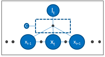
Figure 2: The figure shows a portion of our gated factor graph. The black dots represent the factors across navigation states $x$ and landmark states $l$. The dotted lines represent the gated approach and $c$ is the condition variable.

Factor graphs [25] are graphical models that are well suited to modeling complex estimation problems, such as SLAM. A factor graph is a bipartite graph model comprising two node types: factors $f_{i}\in\mathcal{F}$ and state variables $\theta_{j}\in\Theta$. As shown in Figure 2, there are two kinds of state variable nodes in our factor graph formulation for vision-based SLAM systems: The navigation state nodes $X$ includes the platform information (such as pose and velocity) at all given time steps, while the landmark states $L$ encodes the estimated 3D position of external visual landmarks. Sensor measurements $z_{k}\in Z$ are formulated into factor representations, depending on how a measurement affects the appropriate state variables. For example, a GPS position measurement only involves a navigation state $x$ at a single time. A camera feature observation can involve both a navigation state $x$ and a state of unknown 3D landmark position $l$. Estimating both navigation states and landmark positions simultaneously is very popular in SLAM problem formulation, which is also known as bundle adjustment [26] in computer vision.

The inference process of such a factor graph can be viewed as minimizing the non-linear cost function as follows.

$$\sum_{k=1}^{K}||h_{k}(\Theta_{j_{k}})-\tilde{z_{k}}||_{\Sigma}^{2}$$ (1)

where $h(\Theta)$ is measurement function and and $||\cdot||_{\Sigma}^{2}$ is the Mahalanobis distance with covariance $\Sigma$. There are many efficient solutions to solve this inference process for SLAM systems using the factor graph representation. One popular solution is iSAM2 [27], which uses a Bayes tree data structure to keep all past information and only updates variables influenced by each new measurement. For the details on the factor graph representation and its inference process for SLAM systems, we refer to [28].

Our new gated factor graph framework extends the factor graph representation by modeling the semantic constraint as a gated factor (the dashed lines in Figure 2) in the factor graph for the inference process. As shown in Figure 2, a landmark state $l_{t}$ is only added to the graph to participate the inference process if the condition variable $c$ is $true$. Otherwise this landmark is not used during the inference process in the vision-based SLAM system.

The value on the condition variable $c$ associated with a landmark state is assigned based on the modes of semantic class labels from all observations (2D visual features) on camera images for the same 3D visual landmark (Section 3.1). Note our SegNet architecture generates semantic class label for each pixel on the image and there are total 12 different semantic class labels. However, the same landmark may have different class labels generated by SegNet for its observations across different video frames. Therefore we accumulate the labels among 12 classes for all imaged features correspondent to the same landmark, and decide the Boolean value of the condition variable c for this landmark based on the final counts among all 12 classes. If the landmark is classified as a “valid” semantic class based on the final counts, the condition variable $c$ becomes $true$.

The selection of valid semantic classes for gated factors is different across three perspectives for the navigation system: the feature tracking process, the geo-referenced map building process, and the navigation system using pre-mapped landmarks. We describe how we define the “valid” semantic classes for each situation in the following subsections.

3.3 Visual Feature Tracking

Our framework is able to directly improve real-time navigation performance by enhancing the feature tracking process inside visual SLAM systems (such as [8, 9, 10, 11, 7]). To validate the influence of our approach in pure feature tracking process, we apply our framework on top of the popular ORB-SLAM2 system [7], which cannot incorporate GPS or pre-built geo-referenced maps for navigation.

For each of the tracked features identified on the current video frame from [7], our gated factor graph framework (Figure 2) makes inlier/outlier decision based on the modes of semantic class labels from all 2D imaged positions tracked on past frames of the same tracked feature. Visual features identified as non-static (such as Pedestrian, Vehicle, Bike) or far-away classes (such as Sky) are rejected, and will not contribute to the navigation solution in visual SLAM systems.

3.4 Geo-Referenced Map Building

For high-precision vision-based vehicle navigation systems (such as [6, 16]), our framework improves both the mapping quality beforehand and the localization process using pre-mapped visual landmarks. For demonstration, we implemented our framework on top of the visual-inertial navigation system from [6]. This system builds a high-quality, fully-optimized map of visual landmarks beforehand using IMU, GPS, and one monocular camera. Our gated factor graph for this geo-referenced mapping process is shown in Figure 3. Note there are GPS measurements (green factors in Figure 3) used in the mapping process.

We integrated our semantic segmentation module which classifies imaged regions on input video frames (as shown in Figure 1) into this system [6]. This system uses a landmark matching module to construct the keyframe database, which is used to match features across images to the key frame database. It also has a visual odometry module which generates the features to track across sequential video frames, and passes these features to both the landmark matching module and the inference engine. Our semantic segmentation module receives information about the tracked landmarks from the landmark matching module, and generates the values for the $c$ for the associated landmark constraints to the inference engine, as shown in Figure 3. Note only the 2D-3D visual landmarks from selected semantic classes are preserved in our map. The map of all 2D-3D semantic visual landmarks is then generated and optimized.

The semantic class label of the landmark is computed by using the mode of the labels from all tracked 2D imaged features of the same 3D landmark. The value of the semantic categories is determined empirically. The classes for visual landmarks that were found to be most useful for mapping were Pole, Road Marking, Pavement, Sign Symbol, Tree, Building, Fence. The semantic class labels that were rejected for landmark selection were Sky, Pedestrian, Vehicle, Bike, Road. This makes sense since the rejected classes of landmarks are associated with non-static or far away objects. The road often does not add much value visually since most of the extracted features from the road are typically associated with shadows, which change over time.

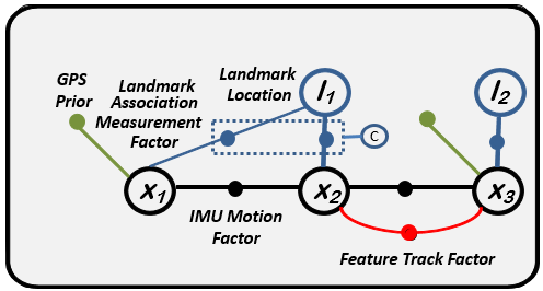
Figure 3: The figure above shows a section of our constructed factor graph for the pre-mapping process in the system from [6]. Factors are formed using measurements from GPS, IMU, and feature tracks. Note factors formed from different kinds of sensor measurements are shown as different colors. The black bubbles represent the state denoted $x$ and the green bubbles represent a prior. The blue dots represent measurements and the blue bubbles represent $l$ states. The dotted lines represent our gated approach and $c$ is the condition variable.

3.5 High-Precision GPS-Denied Navigation

After the landmark database generated from the pipeline in Figure 3, GPS-denied navigation problem reduces to estimate only the pose at the current time in the system from [6]. The pre-built database is used by the landmark matching module to match features tracked from the visual odometry module on new perceived video frames, and provides absolute 2D-3D corrections through pre-mapped visual landmarks in the inference engine. Note the tracked features are also passed from visual odometry module to our semantic segmentation module. This allows our semantic segmentation module to generate the condition variable $c_{i}$values for all the constraints associated with the tracked features during GPS-denied navigation, as shown in Figure 4. Only visual features from selected semantic classes are used in the inference engine.

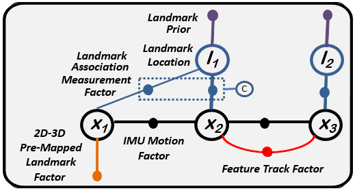
Figure 4: The figure above shows a section of our constructed factor graph for the GPS-denied navigation system from [6] using pre-mapped semantic visual landmarks. Factors are formed using measurements from IMU, feature tracks, and pre-mapped visual landmark observations. Note factors formed from different kinds of sensor measurements are shown as different colors. The black bubbles represent the state denoted $x$ and the green, orange and purple bubbles represent a prior. The blue dots represent measurements and the blue bubbles represent $l$ states. The dotted lines represent the gated approach and $c$ is the condition variable.

Our framework with the GPS-denied navigation system from [6] is visualized in Figure 5. The pictures on the left show the current image and the segmentation from our semantic segmentation module for that image. The estimated trajectory generated from our system is visualized in green, and the red trajectory shows the ground truth for this sequence.

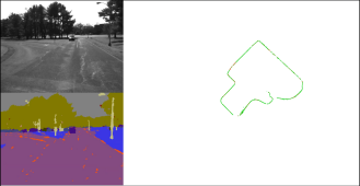
Figure 5: The figure above shows the visualization of the system. The image on the top left is the current frame, and the bottom left is the segmentation for that image. On the right, the trajectory visualized in green is the estimated trajectory generated by our system and the red trajectory shows the ground truth for this sequence.

4 Experimental Evaluation

We validated our framework on top of two vision-based vehicle navigation systems [6, 7], as described in Section 3. Based on the different characteristics of these two systems, we conducted our experiments on various data sets to demonstrate that our approach is able to utilize the semantic information to improve the quality of the navigation solution from different perspectives.

4.1 Feature Tracking for Navigation without Pre-Built Maps

To demonstrate the improvement in feature tracking using our method, we modified the ORB-SLAM2 system [7] (Section 3.3) which uses stereo camera input on the publicly available sequences (sequences 00 - 10) from the KITTI localization benchmark [29] without the use of pre-built maps. We keep the same configuration for all sequences, and use the same configuration for both the baseline performance and the results generated by combining our method with [7]. The parameters chosen for this configuration were 2000 features, 1.2 scale factor, and 8 levels in the scale pyramid. The initial FAST threshold is 12, and the minimum FAST threshold is 7.

Note among these 11 KITTI sequences, there are 6 open-loop sequences which cannot leverage the simultaneous on-the-fly mapping capability from [7] to correct drift when closing the loops during navigation. For these open-loop sequences, the navigation accuracy is purely decided by the visual feature tracking quality. As shown in Table 3, our approach reduces approximately 0.1% drift rate over 9.195 km distance by removing wrong tracked features for these open-loop sequences. It also improves accuracy for sequences with loop-closure optimization.

Table 3: The table below shows our approach reduces the drift rate and mean final location error of the ORB-SLAM2 system for 6 open-loop sequences (open-loop), 5 sequences with loop closures (closed-loop), and all 11 sequences (overall) respectively.

	Location drift rate		Mean Final Location Error
Location drift rate	ORB-SLAM2 (%)	ORSB-SLAM2+Ours (%)	ORB-SLAM2 (m)	ORB-SLAM2 + Ours
Open-Loop	1.6103	1.5234	24.6778	23.3461
Closed-Loop	0.5369	0.5292	13.7130	13.5164
Overall	0.9862	0.9453	19.6938	18.878

Figure 6 shows the qualitative improvement in one of the KITTI open-loop sequences (sequence 09). For this sequence, there are moving vehicles in both directions during driving. Our method avoids the use of tracked features on moving vehicles in ORB-SLAM2 system, and shows clear improvement over the standard ORB-SLAM2 performance . For this sequence, the final error in location without semantic selection is 12.6363 meters whereas the final location error is 3.9253 meters with out method. The total trajectory distance for this sequence is 1.71 km.

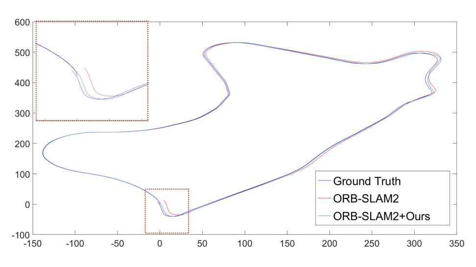
Figure 6: The qualitative improvement (visualized in color) on KITTI sequence 09, using our approach on top of ORB-SLAM2 system. The x and y axes are in meters.

4.2 Landmark Matching Using Semantic Selection

To demonstrate our framework for high-precision vehicle navigation applications using pre-built maps, we applied our framework on top of the system from [6]. We collected data across seasons within same large-scale urban environments which include a variety of buildings, highway driving, and lighting variations. The vehicle we used for experiments incorporates a 100Hz MEMS Microstrain GX4 IMU and one 20Hz front-facing monocular Point Grey camera. High-precision differential GPS, which is also installed on the vehicle, was used both for geo-referenced map construction and for ground truth generation (fused with IMU) to evaluate our GPS-denied navigation system. All three sensors are calibrated and triggered through hardware synchronization. Note for testing this system, we are not aware of any publicly available vehicle data that provides raw IMU and differential GPS measurements with forward-facing camera inputs across season changes at the same place.

The total driving distance is 5.6 km and the total driving time is around 10 minutes for each of the test sequences. Representative images from the test sequences can be seen in Figure 7. Three sequences are used for our experiments, and they are collected by driving in a clockwise loop along the same path around the campus. The database for all experiments is constructed from one data sequence collected in the morning on a partly cloudy day in winter.

Table 4: The table below shows the improvement in the landmark matching module between using the semantic selection of the landmarks and traditional landmark matching. The 3D mean/std error is from the camera re-sectioning error given the pre-mapped 3D locations from the database sequence.

3D Position Accuracy	Without Semantic Selection (meter: mean/std deviation)	With Semantic Selection (meter: mean/std deviation)
Winter, Partly Cloudy Morning	1.871 / 5.745	1.457 / 3.756
Winter, Partly Cloudy Noon	2.084 / 5.851	1.586 / 3.141
Spring, Sunny Morning	1.405 / 0.992	1.140 / 0.476

Table 5: The table below shows the 3D RMS error, 3D Median error, 3D 90 percentile error in the visual-inertial navigation solution with/ without semantic landmark selection.

	3D RMS Error		3D Median Error		3D 90 percentile error
	without semantic (m)	with semantic selection (m)	without semantic (m)	with semantic selection (m)	without semantic (m)	with semantic selection (m)
Winter Partly Cloudy Noon	0.5378	0.4207	0.3532	0.2856	0.7878	0.6109
Spring Sunny Morning	1.1300	0.9640	0.7077	0.6227	1.8656	1.5476

(a)

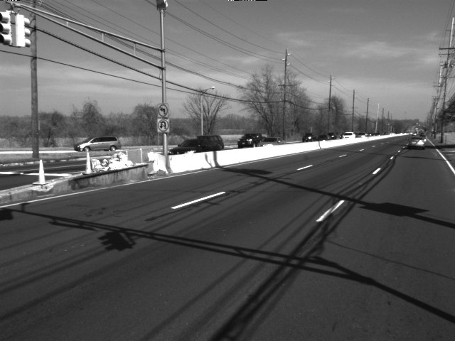
(b)

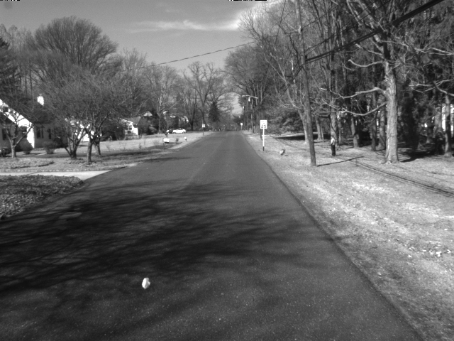
(c)

Figure 7: The figures above show representative images in the sequences. The figure on the far left shows an image where there are trees on both sides and no dynamic objects in the scene. The middle images shows cars on both sides and is on the highway, the right image shows houses on both sides and parked cars. These 3 types of environments are present in all the test sequences used in the experiments.

In this experiment, we evaluate the camera re-sectioning error and the improvement that can be only gained by using semantic selection for the pre-mapped visual landmarks. The results of this experiment are shown in Table 4. As can be seen from Table 4, the overall accuracy in the 3D error is reduced by approximately 30 cm in all sequences and the standard deviation is compressed in all the sequences which shows the improved robustness of the system across seasonal variations using our approach for semantic selection.

Note the camera resection error is computed using all the matched 2D-3D landmarks from the same single key frame stored in the database. All landmarks with different 3D estimated uncertainty are treated equally to compute the camera resection error. There are also outliers in landmark matching results, which increase the error.

4.3 Navigation Using Semantic Pre-Mapped Landmarks

In this evaluation, we measure 3 error metrics to show the improvement by using our semantic selection module for the entire visual inertial navigation solution. Note there are some portions in the test sequence where there are few or no pre-mapped landmarks available due to occlusion or scene changes. However, the navigation system from [6] continuously estimates 3D global pose by tightly fusing IMU data, local tracked features from a monocular camera, and global landmark points from associations between new observed features and pre-mapped visual landmarks. It treats each new observation of a pre-mapped visual landmark as a single measurement instead of computing only one pose measurement from all landmark observations (such as in Section 4.2) at a given time. This way tightly incorporates geo-referenced information into landmark measurements, and is capable of propagating precise 3D global pose estimates for longer periods in GPS-denied setting, which results lower error than pure landmark matching error in Section 4.2.

The 3D RMS error from our GPS-denied navigation solutions is computed across the whole test sequence and is compared to the ground truth generated by the solution using differential GPS and the IMU. We compare our solution using semantic information to the solutions presented by [6]. The first metric is the 3D root mean square error for the trajectory with and without the semantic selection module. As can be seen in Table 5, there is 21% improvement in the 3D RMS error. Table 5 also shows the 3D median error and the 90 percentile error. As can be seen, our approach improves the 3D Median error of the navigation solution by 19.1% and improves the 3D 90 percentile error by 22%.

5 Conclusions

In this paper, we present our framework to improve GPS-denied vehicle navigation accuracy in large-scale urban environments, using semantic information associated with visual landmarks. Our framework utilizes the semantic information to improve the quality of the navigation solution from three perspectives: the feature tracking process, the geo-referenced map building process, and the navigation system using pre-mapped landmarks. In comparison to previous state of the art techniques, we show an improvement of around $20\%$ accuracy which is significant for the precise vehicle navigation applications using pre-mapped visual landmarks.

Compared to other semantic localization and mapping efforts, we present a simple and yet effective approach to both construct landmark databases and to perform localization. This could be further augmented by incorporating cues from other types of information and is not limited to semantic segmentation. We are also not dependent on using a single technique for segmentation and this can be replaced by other techniques as the state of the art improves.

For future work, we plan to accumulate better maps by aggregating physically close features using their semantic labels and enhance the visual map construction by intelligently gathering data from multiple collections. Since we are already able to separate visual features that are associated with permanent objects, the accuracy would only improve with multiple runs since we can aggregate different information to update the label associated with the landmark. We also plan on experimenting with deep learned features in our system, that can be trained to extract both a visual descriptor and a category label for the landmark.

References

- [1] E. Guizzo, “How google’s self-driving car works,” IEEE Spectrum Online, October, vol. 18, 2011.
- [2] J. Levinson and S. Thrun, “Robust vehicle localization in urban environments using probabilistic maps,” in Robotics and Automation (ICRA), 2010 IEEE International Conference on. IEEE, 2010, pp. 4372–4378.
- [3] V. Badrinarayanan, A. Handa, and R. Cipolla, “Segnet: A deep convolutional encoder-decoder architecture for robust semantic pixel-wise labelling,” arXiv preprint arXiv:1505.07293, 2015.
- [4] C. Cadena, L. Carlone, H. Carrillo, Y. Latif, D. Scaramuzza, J. Neira, I. D. Reid, and J. J. Leonard, “Simultaneous localization and mapping: Present, future, and the robust-perception age,” arXiv preprint arXiv:1606.05830, 2016.
- [5] S. Choudhary, A. J. Trevor, H. I. Christensen, and F. Dellaert, “Slam with object discovery, modeling and mapping,” in IROS 2014, 2014.
- [6] H.-P. Chiu, M. Sizintsev, X. S. Zhou, P. Miller, S. Samarsekera, and R. T. Kumar, “Sub-meter vehicle navigation using efficient pre-mapped visual landmarks,” in International Conference on Intelligent Transport Systems, 2016.
- [7] R. Mur-Artal, J. Montiel, and J. Tardós, “Orb-slam: A versatile and accurate monocular slam system,” IEEE transactions on robotics, vol. 31, no. 5, pp. 1147–1163, 2015.
- [8] H. Durrant-Whyte and T. Bailey, “Simultaneous localization and mapping: part i,” IEEE robotics & automation magazine, vol. 13, no. 2, pp. 99–110, 2006.
- [9] J. Fuentes-Pacheco, J. Ruiz-Ascencio, and J. M. Rendón-Mancha, “Visual simultaneous localization and mapping: a survey,” Artificial Intelligence Review, vol. 43, no. 1, pp. 55–81, 2015.
- [10] A. J. Davison, I. D. Reid, N. D. Molton, and O. Stasse, “Monoslam: Real-time single camera slam,” IEEE transactions on pattern analysis and machine intelligence, vol. 29, no. 6, pp. 1052–1067, 2007.
- [11] A. J. Davison, “Real-time simultaneous localisation and mapping with a single camera,” in Computer Vision, 2003. Proceedings. Ninth IEEE International Conference on. IEEE, 2003, pp. 1403–1410.
- [12] H.-P. Chiu, S. Williams, F. Dellaert, S. Samarasekera, and R. Kumar, “Robust vision-aided navigation using sliding-window factor graphs,” in Robotics and Automation (ICRA), 2013 IEEE International Conference on. IEEE, 2013, pp. 46–53.
- [13] S. Leutenegger, S. Lynen, M. Bosse, R. Siegwart, and P. Furgale, “Keyframe-based visual–inertial odometry using nonlinear optimization,” The International Journal of Robotics Research, vol. 34, no. 3, pp. 314–334, 2015.
- [14] N. D. Reddy, P. Singhal, V. Chari, and K. M. Krishna, “Dynamic body vslam with semantic constraints,” in Intelligent Robots and Systems (IROS), 2015 IEEE/RSJ International Conference on. IEEE, 2015, pp. 1897–1904.
- [15] A. Kundu, Y. Li, F. Dellaert, F. Li, and J. M. Rehg, “Joint semantic segmentation and 3d reconstruction from monocular video,” in European Conference on Computer Vision. Springer, 2014, pp. 703–718.
- [16] C. Beall and F. Dellaert, “Appearance-based localization across seasons in a metric map,” 6th PPNIV, Chicago, USA, 2014.
- [17] P. F. Alcantarilla, S. Stent, G. Ros, R. Arroyo, and R. Gherardi, “Street-view change detection with deconvolutional networks,” in Robotics: Science and Systems, 2016.
- [18] S. Choudhary, V. Indelman, H. I. Christensen, and F. Dellaert, “Information-based reduced landmark slam,” in 2015 IEEE International Conference on Robotics and Automation (ICRA). IEEE, 2015, pp. 4620–4627.
- [19] J. Biswas and M. Veloso, “Episodic non-markov localization: Reasoning about short-term and long-term features,” in 2014 IEEE International Conference on Robotics and Automation (ICRA). IEEE, 2014, pp. 3969–3974.
- [20] D. Meyer-Delius, J. Hess, G. Grisetti, and W. Burgard, “Temporary maps for robust localization in semi-static environments,” in Intelligent Robots and Systems (IROS), 2010 IEEE/RSJ International Conference on. IEEE, 2010, pp. 5750–5755.
- [21] H. Lategahn, M. Schreiber, J. Ziegler, and C. Stiller, “Urban localization with camera and inertial measurement unit,” in 2013 IEEE Intelligent Vehicles Symposium (IV). IEEE, 2013.
- [22] G. J. Brostow, J. Fauqueur, and R. Cipolla, “Semantic object classes in video: A high-definition ground truth database,” Pattern Recognition Letters, vol. 30, no. 2, pp. 88–97, 2009.
- [23] C. Tai, T. Xiao, Y. Zhang, X. Wang, and E. Weinan, “Convolutional neural networks with low-rank regularization,” in 2016 International Conference on Learning Representations (ICLR), 2016.
- [24] T. Minka and J. Winn, “Gates,” in Advances in Neural Information Processing Systems, 2009, pp. 1073–1080.
- [25] F. Kschischang, B. Fey, and H. Loeliger, “Factor graphs and the sum-product algorithm,” IEEE Trans. Information Theory, vol. 47, no. 2, 2001.
- [26] B. Triggs, P. F. McLauchlan, R. I. Hartley, and A. W. Fitzgibbon, “Bundle adjustment - a modern synthesis,” Lecture Notes in Computer Science, vol. 1883, pp. 298–375, 2000.
- [27] M. Kaess, H. Johannsson, R. Roberts, V. Ila, J. Leonard, and F. Dellaert, “isam2: Incremental smoothing and mapping using the bayes tree,” Intl. J. of Robotics Research, vol. 31, pp. 217–236, 2012.
- [28] F. Dellaert, “Factor graphs and gtsam: A hands-on introduction,” in Georgia Institute of Technology, 2012.
- [29] A. Geiger, P. Lenz, and R. Urtasun, “Are we ready for autonomous driving? the kitti vision benchmark suite,” in Computer Vision and Pattern Recognition (CVPR), 2012 IEEE Conference on. IEEE, 2012, pp. 3354–3361.