Mobility and Congestion in Dynamical Multilayer Networks with Finite Storage Capacity

Abstract

Multilayer networks describe well many real interconnected communication and transportation systems, ranging from computer networks to multimodal mobility infrastructures. Here, we introduce a model in which the nodes have a limited capacity of storing and processing the agents moving over a multilayer network, and their congestions trigger temporary faults which, in turn, dynamically affect the routing of agents seeking for uncongested paths. The study of the network performance under different layer velocities and node maximum capacities, reveals the existence of delicate trade-offs between the number of served agents and their time to travel to destination. We provide analytical estimates of the optimal buffer size at which the travel time is minimum and of its dependence on the velocity and number of links at the different layers. Phenomena reminiscent of the Slower Is Faster (SIF) effect and of the Braess’ paradox are observed in our dynamical multilayer set-up.

Extensive studies on congestion phenomena in complex networks latora_nicosia_russo_2017 have highlightened the role of routing strategies Echenique  et al. (2004, 2005); Scellato  et al. (2010); Wang  et al. (2014); Lima  et al. (2016); Yan  et al. (2006) and network topologies De Domenico  et al. (2014); Duch and Arenas (2007); Crucitti  et al. (2004); De Domenico  et al. (2014); Duch and Arenas (2007) on the propagation of faults and on the emergence of congestion Guimerà  et al. (2002); Çolak  et al. (2016); De Domenico  et al. (2015); De Martino  et al. (2009); Yang  et al. (2009). Recently, multilayer network models have been introduced to better describe complex systems composed of interconnected networks Kivelä  et al. (2014); De Domenico  et al. (2013); Morris and Barthélemy (2012); Manfredi (2017). Diffusion processesGómez  et al. (2013); Granell  et al. (2013); Nicosia  et al. (2017) and congestion have also been explored in the context of multilayer networks Ren  et al. (2014); Chodrow  et al. (2016). For instance, Ref. Solé-Ribalta  et al. (2016) has shown that multiplexity can induce congestions that otherwise would not appear if the individual layers were not interconnected. Also the effects on congestion of the mechanism of changing layer as a function of the velocities of the links of two layers has been analyzed Morris and Barthélemy (2012). However, essential aspects of the dynamics of congestions, which can play even a more important role in multilayer systems, are still missing. Firstly, nodes and links have been treated as static entities, in the sense that the dynamical effects of the congestion on the node queue length and agents’ routing have not been explicitely considered Morris and Barthélemy (2012); Strano  et al. (2015); Solé-Ribalta  et al. (2016); Chodrow  et al. (2016). Secondly, the capacity of storing agents or packets at nodes has usually been assumed infinite Solé-Ribalta  et al. (2016), neglecting the dynamical evolution of a node to be available or unavaible during time according to whether its queue is uncongested or congested, respectively.

In this Letter, we introduce a multilayer mobility model capturing both the dynamic nature of the queues at the network nodes, and also the consequent congestion phenomena induced by the limited storage capacity, i.e. finite buffer size, of the nodes of any real multilayer system. Our model well describes the mechanisms of congestion occurring at the routers of a multilayer communication network. The main ingredient of the model is that it takes into account that agents seek for uncongested paths during their navigation. This makes the routing strategy of the agents explicitly dependent on the dynamic effects of the congestion at the nodes rather than at the links of the network Echenique  et al. (2004, 2005); Scellato  et al. (2010). Moreover, in our model a node is unavailable when congested and again available when becomes uncongested. Therefore, the onset of congestion triggers a sort of temporary fault of the node and affects the routing of agents, which seek for uncongested paths. In this respect, the model allows to investigate the effect of temporary faults on the performance of a multilayer network, extending the analysis originally performed on single-layer networks, and limited to permanent faults Motter and Lai (2002); Crucitti  et al. (2004); Motter (2004). Finally, the combination of the above dynamical effects yields a coevolving multilayer network due to the circular argument by which the agents’ routing depends on the congestion phenomena and the latter is in turn influenced by the agents’ behavior to seek for uncongested paths. This leads to novel multilayer phenomena characterised by the existence of an optimal value of the node buffer size where the travel time is minimum, and which critically depends on the topologies and on the velocities of the different layers.

The model.  The backbone of our system is modeled as a weighted multilayer network with $L$ layers and $N^{\alpha}$ nodes at layer $\alpha$, with $\alpha=1,2,\ldots,L$. Agents moving on the network can for instance represent information packets in a communication system: they are generated at the nodes of the network and move from a node to one of its neighbours until they arrive at their assigned final destination, where they are removed from the network. The dynamics of the nodes and links is illustrated in Fig.1 of Supp. Mat. The main quantity of interest to characterize the state of node $i$ at layer $\alpha$ and at time $t$, is its queue length $q_{i}^{\alpha}(t)$ which represents the number of agents at the node. Additionally, we assume that each node $i$ at layer $\alpha$ is characterized by its maximum resource $B_{i}^{\alpha}$, representing the node capability to store agents, for instance the buffer size of a router in a computer network. This implies that $q_{i}^{\alpha}(t)\leq B_{i}^{\alpha}$ for all $t$. We also adopt First-In-First-Out (FIFO) queues, which means that agents are processed by the queue at any given node in order of their arrival. The basic assumption of our transportation model is that the agents have a global knowledge of the network Scellato  et al. (2010), and move from their origins to their destinations by following minimum-weight paths. Since our aim is to model the dynamics of agents that try to minimise distances but also to avoid congested nodes Echenique  et al. (2004, 2005); Scellato  et al. (2010), we assume that the link weights depend on the node queue lengths Crucitti  et al. (2004); Kinney  et al. (2005). Namely, the weight $w_{ij}^{\alpha\beta}$ of the link connecting node $i$ at layer $\alpha$ to node $j$ at layer $\beta$ is defined as:

$$w_{ij}^{\alpha\beta}(t)=c\cdot\gamma_{ij}^{\alpha\beta}+\frac{q_{j}^{\beta}(t)}{B_{j}^{\beta}-q_{j}^{\beta}(t)}$$ (1)

where $\gamma_{ij}^{\alpha\beta}$ for $\alpha\neq\beta$ represents the time of going from node $i$ at layer $\alpha$ to node $j$ at layer $\beta$, and $c$ is the equivalent cost per unit time, so that $c\cdot\gamma_{ij}^{\alpha\beta}$ is the intrinsic cost of traversing the link. Similarly, $c\cdot\gamma_{ij}^{\alpha\alpha}$ is the intrinsic cost of link $(i,j)$ in layer $\alpha$. The second term in the right hand side of Eq. (1) represents the cost perceived by the agents and due to the level of congestion found at the node $j$. Notice that $w_{ij}^{\alpha\beta}(t)\in[c\cdot\gamma_{ij}^{\alpha\beta},\infty)$, with the weight of the link from $i$ to $j$ taking its minimum value $c\cdot\gamma_{ij}^{\alpha\beta}$ when the queue at $j$ is empty, i.e. when $q_{j}^{\beta}(t)=0$, while the weight diverges when the queue is full, i.e. when $q_{j}^{\beta}(t)=B_{j}^{\beta}$. At each time step, each agent computes its next move on the network based on the set of weights associated to the links at time $t$. Let us denote as $R_{i}^{\alpha}(t)$ the resulting net flow at node $i$ of layer $\alpha$:

$$R_{i}^{\alpha}(t)=I_{i}^{\alpha}(t)+\delta I_{i}^{\alpha}(t)-O_{i}^{\alpha}(t)-\delta O_{i}^{\alpha}(t),$$ (2)

where $I_{i}^{\alpha}(t)$ and $O_{i}^{\alpha}(t)$ are respectively the queue incoming and outgoing rate from and to other nodes, while $\delta I_{i}^{\alpha}(t)$ and $\delta O_{i}^{\alpha}(t)$ are the number of agents generated or removed at node $i$ and layer $\alpha$, at each time. In particular, the output rate $O_{i}^{\alpha}(t)$ of node $i$ is related to the capacity of the node to serve agents and route them towards other nodes, and we assume that each node $i$ is characterized by a maximum service rate $\hat{O}_{i}^{\alpha}$, such that $O_{i}^{\alpha}(t)\leq\hat{O}_{i}^{\alpha}$. Once all the values of $R_{i}^{\alpha}(t)$ are calculated, we adopt the following update rule of node queues:

$$q_{i}^{\alpha}(t+1)=\begin{cases}0&q_{i}^{\alpha}(t)+R_{i}^{\alpha}(t)\leq 0\\ q_{i}^{\alpha}(t)+R_{i}(t)^{\alpha}&0<q_{i}^{\alpha}(t)+R_{i}^{\alpha}(t)<B_{i}^{\alpha}\\ B_{i}^{\alpha}&B_{i}^{\alpha}\leq q_{i}^{\alpha}(t)+R_{i}^{\alpha}(t)\end{cases}$$ (3)

for each $\alpha=1,\ldots,L$ and $i=1,\ldots,N^{\alpha}$. Notice that the waiting time spent by an agent at node $i$ at time $t$ is ${q_{i}^{\alpha}(t)}/{\hat{O}_{i}^{\alpha}}$, and can take a maximum value of ${B_{i}^{\alpha}}/{\hat{O}_{i}^{\alpha}}$. The model takes into account that agents seek for uncongested paths during their navigation. Moreover, agent loss may also occur in the model because of the congestion (i.e. packet loss in communication networks). Specifically, an agent is lost at a node when it cannot be forwarded to one of the neighbouring nodes because they are all congested. Summing up, the control parameters of our network model are: $B_{i}^{\alpha}$, $\hat{O}_{i}^{\alpha}$, $\gamma_{ij}^{\alpha\beta}$, $\forall i,j,\alpha$ and $\beta$.

Results.  To illustrate the rich dynamical behaviour of the model under different control parameters, we consider a network with two layers ($L=2$) of $N^{1}=150$ and $N^{2}=30$ nodes respectively. The two layers are generated as geometric random graphs by randomly placing the nodes on the unit square and connecting two nodes $i$ and $j$ if their Euclidean distance is $R_{ij}<0.11$ (layer 1) or $0.11\leq R_{ij}\leq 0.19$ (layer 2) Barthélemy (2011); Solé-Ribalta  et al. (2016). The aim is to represent with layer 1 a denser network with high clustering coefficient and short-range connections, and with layer $2$ a network of fewer nodes with long-range connections. We also assume that layer $2$ is a faster transportation system. Hence, we fix $\gamma^{11}_{ij}=\gamma^{11}=1$ and $0<\gamma^{22}_{ij}=\gamma^{22}\leq\gamma^{11}$ $\forall i,j$, so that we can explore different values of the time ratio $\gamma=\gamma^{22}/\gamma^{11}$ in the range $(0,1]$. As the time to traverse a link is inversely proportional to the velocity or bandwidth of the link, in the following we will refer to $\gamma$ as the velocity ratio. We also fix $c=1$, $\gamma^{12}_{ij}=\gamma^{12}=1$, $\hat{O}_{i}^{1}=\hat{O}_{i}^{2}=\hat{O}=640$ and $B_{i}^{1}=B_{i}^{2}=B~{}\forall i,j$. At each time step $t$, and for each node $i$ and layer $\alpha$, we generate with a probability $\rho$ an agent to be delivered to each of the remaining $N^{1}+N^{2}-1$ of the multilayer network, such that $\delta I_{i}^{\alpha}(t)$ is on average equal to $\rho(N^{1}+N^{2}-1)~{}\forall i,\alpha$.

To evaluate the performance of the system we have looked at quantities such as the average travel time and the number of lost agents for various velocity ratios $\gamma\in(0,1]$ and buffer sizes $B$. All the performance indexes are obtained as averages when the network has reached a steady state condition.

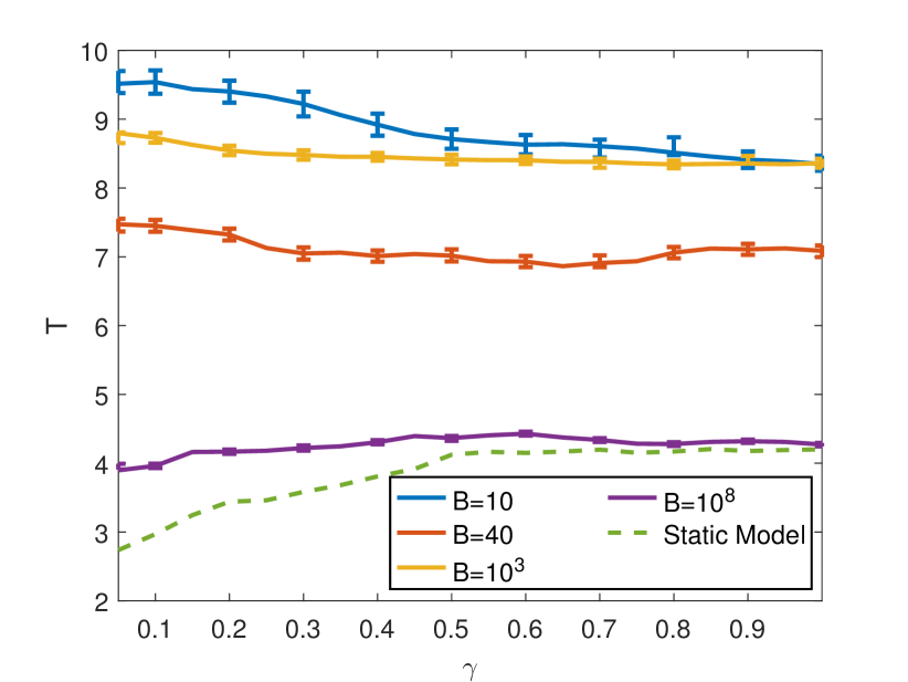
Figure 1: Average travel time $T$ of delivered agents as a function of the velocity ratio $\gamma$ in our dynamic multilayer mobility model with three different values of node buffer size $B=10,40,10^{3},10^{8}$ (continuous lines) and in the corresponding static model (dashed line). Numerical results are reported as symbols, with the error bars representing fluctuations over random agent generations and 100 different network realizations.

Fig. 1 reports the average travel time $T$, defined as $T=1/N_{a}\sum_{a=1}^{N_{a}}(t^{\rm OUT}_{a}-t^{\rm IN}_{a})$, where $t^{\rm OUT}_{a}$ and $t^{\rm IN}_{a}$ are respectively the times at which agent $a$ enters the network and arrives at its destination, and $N_{a}$ is the total number of delivered agents.

The plots of $T$ as a function of $\gamma$ for buffer sizes $B=10,40$ and $10^{3}$ show that the travel time decreases when $\gamma$ increases, i.e. when we decrease the velocity of the faster layer $2$, keeping fixed the velocity of layer $1$. This is an example, in a multilayer set-up, of the Slower Is Faster (SIF) effect reported for several complex systems in the literature and in which the decrease of the velocity can yield to an improvement of the system performance SIF . The increase of $T$ we observe here when $\gamma$ decreases is due to the increasing waiting times $q(t)/\hat{O}$ experimented by agents along the preferential and bottlenecked paths induced by the increasingly different velocities of the two layers. Interestingly, the effect does not occur in a static model not accounting for the queue dynamics Morris and Barthélemy (2012). The results of the static model, reported for comparison as dashed line, show indeed that $T$ decreases for decreasing values of $\gamma$. As expected, our model tends to the dashed line of the static model for very large values of $B$ (see the curve for $B=10^{8}$), since the link weights in Eq. (1) become independent from the queue $q(t)$ when $B\to\infty$.

An analogous of the Braess’s paradox, in which the addition of resources in terms of links leads to a worsening of network performance, shows up in our model in the dependence of $T$ on the buffer (i.e the addition of physical space to the nodes). In fact, when we increase $B$ from 10 to 40 we reduce congestion and agent losses and, as expected, we observe a drop of the travel time (for any value of $\gamma$). However, a further increase of the node buffer size does not lead to an additional improvement of the system, as we observe, for instance at at $B=10^{3}$, an increase of the travel time $T$.

Figure 2: Average travel time $T$ (a), percentage of agent loss $\Lambda$ (b), and (c) maximum betweenness centrality $C^{\rm max}$ for the dynamic multilayer mobility model as functions of the node buffer size $B$, and for three different values of velocity ratio $\gamma=0.05,0.5,1$.

To better highlight the non-monotonous dependence of the average travel time from the node buffer size $B$ observed in Fig. 1, in panel (a) and (b) of Fig. 2 we report $T$ as a function of $B$, together with the agent loss $\Lambda$, defined as the percentage of agents that are unable to reach their destination with respect to the total number of generated agents. We adopt a logarithmic scale for $B$, and we show the results for three different velocity ratios, namely $\gamma=0.05,0.5$ and 1. We first describe the case $\gamma=1$. In the limit $B\to\infty$ the network is uncongested and $\Lambda\to 0$. By decreasing the value of the buffer size, the agent loss $\Lambda$ starts to increase at $B\simeq 10^{2}$ and triggers nodes alternatively being full and empty. In this regime, the average queue length $\bar{q}$ is well approximated by $\bar{q}\simeq B/2$ with an average waiting time ${{\bar{q}}}/{\hat{O}}\simeq B/2\hat{O}$, so that the average travel time $T$ linearly decreases with the buffer size $B$. This behavior holds until a value $B_{T_{\rm min}}\simeq 40$, at which the average travel time $T$ assumes its optimal value. Finally, when the buffer size is reduced to values $B<B_{T_{\rm min}}$, a congestion collapse occurs with a sharp increase of agent loss. In such high-congestion regime, the average travel time $T$ increases because of the high number of alternative but longer paths available. We can notice from panel (c) of Fig. 2 that, for $B\in[40,80]$, the increase in the travel time is related to the increase of the network maximum betweenness centrality $C^{\rm max}$, which is upper bounded by the node buffer size. This is in agreement with the results found in Refs. Danila2006 ; Danila2007 for single-layer networks. When $B>80$, the increase in $T$ is mainly due to the increased waiting time ${q(t)}/{\hat{O}}$ of the agents in a queue, combined with the nonlinear dynamics of link weights. Conversely, the maximum betweenness centrality $C^{\rm max}$ decreases, as the agents go through a lower number of more congested nodes. The curves for $\gamma<1$ reported in Fig. 2 indicate in general a worsening of the travel time $T$ with respect to the case $\gamma=1$. Specifically, for $B\gg B_{T_{\rm min}}$, the increase of the average travel time $T$ is due to the increase of the waiting time $q(t)/\hat{O}$ on preferential paths which gives rise to the Braess’ paradox observed already in Fig.  1. For low value of buffer size $B\ll B_{T_{\rm min}}$, lower value of $\gamma$ makes the faster layer more and more preferential and congested such that the paths crossed by the agents include a larger number of links and nodes of the slower layer. The effect is an increase of $T$ for decrease of $\gamma$. In this case the number of agent loss is almost the same but it is differently distributed along the multilayer networks, with most occurring at the fast layer.

Differently, for buffer sizes around $B_{T_{\rm min}}$, as shown in the inset, the average time $T$ is lower for higher velocity (lower $\gamma$) as in the case of the static model. This is because the waiting time $q(t)/\hat{O}$ can be neglected with respect to the intrinsic time to traverse a link.

Analytical estimations of $B_{T_{\rm min}}$.  The most striking result of our model with finite storing capacity is that the optimal value $B_{T_{\rm min}}$ of the buffer depends on the velocities of the layers of the multilayer. It is therefore of outmost importance to obtain an analytical expression of $B_{T_{\rm min}}$ as a function of $\gamma$. We observe that, under standard working conditions, the network is characterized by a steady state in which the number of generated agents equals the number of agents leaving the network at their destination. By the Little’s law Little and Graves (2008) we can then write:

$$Q=\frac{N{\bar{q}}}{\bar{\tau}}$$ (4)

where $Q$ is the total generated traffic per unit time, $\bar{q}$ is the average queue length, $\bar{\tau}$ is the average time spent by the agent over the network, and $N=N^{1}+N^{2}$. To evaluate $\bar{\tau}$, consider that on average the time spent by an agent from the output of a node $i$ to the output of its neighbour $j$ is $\bar{\gamma}+{{\bar{q}}}/{\hat{O}}$, namely the sum of the average intrinsic time to cover the link $(i,j)$ and the average waiting time at the queue ${{\bar{q}}}/{\hat{O}}$. The value $\bar{\gamma}$ can be evaluated as $\bar{\gamma}=\frac{\gamma^{11}K^{1}+\gamma^{22}K^{2}+\gamma^{12}K^{12}}{K^{1}+K^{2}+K^{12}}$, where $K^{12}$, $K^{1}$ and $K^{2}$ are respectively the number of interlinks and of links in the two layers. Hence, the average time spent by an agent on a typical path is $\bar{\tau}=\bar{h}(\bar{\gamma}+\frac{{\bar{q}}}{\hat{O}})$ where $\bar{h}$ is the average number of links on the shortest path. Since the buffer $B_{T_{\rm min}}$ is associated to the onset of the network congestion collapse, i.e. when all queues are full and we have $\bar{q}/B_{T_{\rm min}}\simeq 1$, by plugging the expression of $\bar{\tau}$ in Eq. (4) and solving it for $\bar{q}$, we get the following estimate for the minimum buffer size:

$$B_{T_{\rm min}}\simeq\bar{q}=\frac{\bar{\gamma}Q\overline{h}}{N-\frac{Q\overline{h}}{\hat{O}}}$$ (5)

In particular, for the case considered in our simulations, we have $N=120$, $\overline{h}=4.1$, $Q=N(N-1)\rho$ with $\rho=0.08$, and $\hat{O}=500$. For $\gamma=0.05$, $\gamma=0.5$ and $\gamma=1$ we get respectively $B_{T_{\rm min}}\simeq 35$, $B_{T_{\rm min}}\simeq 38$ and $B_{T_{\rm min}}\simeq 42$. These values are reported as vertical lines in the inset of Fig. 2 and are in good agreement with the optimal values obtained numerically. Eq. (5) highlights that a faster multilayer network, i.e. one with lower $\bar{\gamma}$, has a lower $B_{T_{\rm min}}$. This is well confirmed by Fig. 3, where we report both the numerically derived and the analytical prediction of $B_{T_{\rm min}}$ as function of $\gamma$ for multilayer networks with different values of $K^{1}$ and $K^{2}$. We observe that the variation of $B_{T_{\rm min}}$ as a function of $\gamma$ is larger when fast and slow layers have a similar number of links. On the other hand, when the fast layer has much fewer links than the slow layer, the value of $B_{T_{\rm min}}$ of the multilayer network is almost independent on the difference of the layer velocity. This also suggests that even a slight improvement in the velocity of links of the denser layer can have better effects on $B_{T_{\rm min}}$ than speeding up or adding new links to the faster layer.

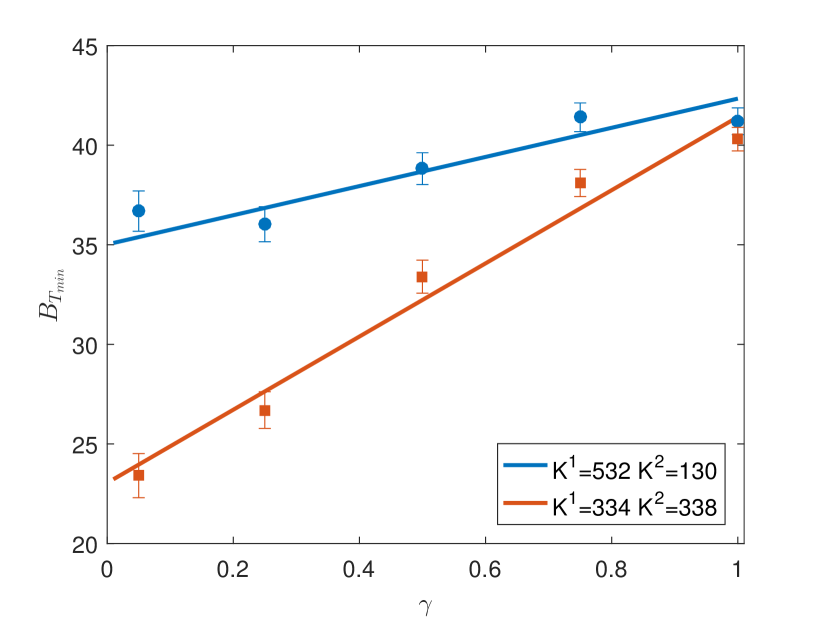
Figure 3: Optimal buffer values $B_{T_{\rm min}}$ as a function of the velocity ratio $\gamma$ and for two multilayers (the first with $K^{1}=532$ and $K^{2}=130$ is the one considered in the previous figures, while the second has $K^{1}=K^{2}=334$). Numerical results are reported as symbols, with the error bars representing fluctuations over random agent generations and 100 different network realizations, while the continuous lines are the theoretical predictions of Eq. (5).

The analytical estimate of $B_{T_{\rm min}}$ provided in this Letter can be useful to design efficient multilayer mobility systems. In particular, the model shows that an increase of network resources in terms of the link velocities or of the buffer sizes can surprisingly lead to a worsening of the performance. The first behavior is reminiscent of the SIF effect SIF while the latter is an analogous of the Braess’ paradox originally defined for single layer networks Valiant and Roughgarden (2010) and recently observed in multiplex networks as a function of the layer average degrees Solé-Ribalta  et al. (2016). Here we found both effects in dynamical multilayer mobility networks with finite storing capacity.

- (1) V. Latora, V. Nicosia, G. Russo, Complex Networks: Principles, Methods and Applications, Cambridge University Press (2017).
- Echenique et al. (2004) P. Echenique, J. Gómez-Gardeñes, and Y. Moreno, Phys. Rev. E 70, 056105 (2004).
- Echenique et al. (2005) P. Echenique, J. Gómez-Gardeñes, and Y. Moreno, EPL (Europhysics Letters) 71, 325 (2005).
- Scellato et al. (2010) S. Scellato, L. Fortuna, M. Frasca, J. Gómez-Gardeñes, and V. Latora, The European Physical Journal B 73, 303 (2010).
- Wang et al. (2014) P. Wang, L. Liu, X. Li, G. Li, and M. C. González, New Journal of Physics 16, 013012 (2014).
- Lima et al. (2016) A. Lima, R. Stanojevic, D. Papagiannaki, P. Rodriguez, and M. C. González, Journal of The Royal Society Interface 13, 20160021 (2016).
- Yan et al. (2006) G. Yan, T. Zhou, B. Hu, Z.-Q. Fu, and B.-H. Wang, Phys. Rev. E 73, 046108 (2006).
- De Domenico et al. (2014) M. De Domenico, A. Solé-Ribalta, S. Gómez, and A. Arenas, PNAS 111, 8351 (2014).
- Duch and Arenas (2007) J. Duch and A. Arenas, in Proc. SPIE, Vol. 6601 (2007) pp. 66010O–66010O–8.
- Crucitti et al. (2004) P. Crucitti, V. Latora, and M. Marchiori, Phys. Rev. E 69, 045104 (2004).
- Guimerà et al. (2002) R. Guimerà, A. Díaz-Guilera, F. Vega-Redondo, A. Cabrales, A. Arenas, Phys. Rev. Lett. 89, 248701 (2002).
- Çolak et al. (2016) S. Çolak, A. Lima, and M. C. González, Nature communications 7 (2016).
- De Domenico et al. (2015) M. De Domenico, A. Lima, M. C. González, and A. Arenas, EPJ Data Science 4, 1 (2015).
- De Martino et al. (2009) D. De Martino, L. Dall’Asta, G. Bianconi, and M. Marsili, Phys. Rev. E 79, 015101 (2009).
- Yang et al. (2009) R. Yang, W.-X. Wang, Y.-C. Lai, and G. Chen, Phys. Rev. E 79, 026112 (2009).
- Kivelä et al. (2014) M. Kivelä, A. Arenas, M. Barthélemy, J. P. Gleeson, Y. Moreno, and M. A. Porter, Journal of complex networks 2, 203 (2014).
- De Domenico et al. (2013) M. De Domenico, A. Solé-Ribalta, E. Cozzo, M. Kivelä, Y. Moreno, M. A. Porter, S. Gómez, and A. Arenas, Phys. Rev. X 3, 041022 (2013).
- Morris and Barthélemy (2012) R. G. Morris and M. Barthélemy, Phys. Rev. Lett. 109, 128703 (2012).
- Manfredi (2017) S. Manfredi, Multilayer Control of Networked Cyber-Physical Systems. (Advances in Industrial Control Series, Springer, 2017).
- Gómez et al. (2013) S. Gómez, A. Díaz-Guilera, J. Gómez-Gardeñes, C. J. Pérez-Vicente, Y. Moreno, and A. Arenas, Phys. Rev. Lett. 110, 028701 (2013).
- Granell et al. (2013) C. Granell, S. Gómez, and A. Arenas, Phys. Rev. Lett. 111, 128701 (2013).
- Nicosia et al. (2017) V. Nicosia, P. S. Skardal, A. Arenas, and V. Latora, Phys. Rev. Lett. 118, 138302 (2017).
- Ren et al. (2014) Y. Ren, M. Ercsey-Ravasz, P. Wang, M. C. González, and Z. Toroczkai, Nature Communications 5 (2014).
- Chodrow et al. (2016) P. S. Chodrow, Z. Al-Awwad, S. Jiang, and M. C. González, PLoS one 11, e0161738 (2016).
- Solé-Ribalta et al. (2016) A. Solé-Ribalta, S. Gómez, and A. Arenas, Phys. Rev. Lett. 116, 108701 (2016).
- Strano et al. (2015) E. Strano, S. Shai, S. Dobson, and M. Barthélemy, Journal of The Royal Society Interface 12, 20150651 (2015).
- Motter and Lai (2002) A. E. Motter and Y.-C. Lai, Phys. Rev. E 66, 065102 (2002).
- Motter (2004) A. E. Motter, Phys. Rev. Lett. 93, 098701 (2004).
- Kinney et al. (2005) R. Kinney, P. Crucitti, R. Albert, and V. Latora, The European Physical Journal B 46, 101 (2005).
- Barthélemy (2011) M. Barthélemy, Physics Reports 499, 1 (2011).
- (31) B. Danila, Y. Yu, J. A. Marsh, and K. E. Bassler, Phys. Rev. E 74, 046106 (2006).
- (32) B. Danila, Y. Yu, J. A. Marsh, and K. E. Bassler, Chaos 17, 026102 (2007).
- Little and Graves (2008) J. D. Little and S. C. Graves, in Building intuition (Springer, 2008) pp. 81–100.
- Valiant and Roughgarden (2010) G. Valiant and T. Roughgarden, Random Structures & Algorithms 37, 495 (2010).
- (35) C. Gershenson and D. Helbing, Complexity 21, 9 (2015).