Brightest group galaxies-II: the relative contribution of BGGs to the total baryon content of groups at $z<1.3$

Abstract

We performed a detailed study of the evolution of the star formation rate (SFR) and stellar mass of the brightest group galaxies (BGGs) and their relative contribution to the total baryon budget within $R_{200}$ ($f^{BGG}_{b,200}$). The sample comprises 407 BGGs selected from X-ray groups ($M_{200}=10^{12.8}-10^{14}\;M_{\odot}$) out to $z\sim 1.3$ identified in the COSMOS, XMM-LSS, AEGIS fields. We find that BGGs constitute two distinct populations of quiescent and star-forming galaxies and their mean SFR is $\sim 2$ dex higher than the median SFR at $z<1.3$. Both the mean and the median SFRs decline with time by $>2$ dex. The mean (median) of stellar mass has grown by $0.3$ dex since $z=1.3$ to the present day. We show that up to $\sim 45\%$ of the stellar mass growth in a star-forming BGG can be due to its star-formation activity. With respect to $f^{BGG}_{b,200}$, we find it to increase with decreasing redshift by $\sim 0.35$ dex while decreasing with halo mass in a redshift dependent manner. We show that the slope of the relation between $f^{BGG}_{b,200}$ and halo mass increases negatively with decreasing redshift. This trend is driven by an insufficient star-formation in BGGs, compared to the halo growth rate. We separately show the BGGs with the 20% highest $f^{BGG}_{b,200}$ are generally non-star-forming galaxies and grow in mass by processes not related to star formation (e.g., dry mergers and tidal striping). We present the $M_{\star}-M_{h}$ and $M_{\star}/M_{h}-M_{h}$ relations and compare them with semi-analytic model predictions and a number of results from the literature. We quantify the intrinsic scatter in stellar mass of BGGs at fixed halo mass ($\sigma_{logM_{\star}}$) and find that $\sigma_{logM_{\star}}$ increases from 0.3 dex at $z\sim 0.2$ to 0.5 dex at $z\sim 1.0$ due to the bimodal distribution of stellar mass.

1 Introduction

The baryon content of the universe and its partitioning between different components, e.g., hot/cold gas and stars, is one of the most important observations in cosmology. Clusters of galaxies are thought to have baryon fractions that approach the cosmic mean, with most of the baryons in the form of x-ray emitting hot gas and stars, and are particularly important in this context (White & Frenk, 1991). This has been confirmed by previous studies which found that, after including baryons in stars, the baryon content in the most massive clusters closely matches that measured from observations of the CMB (White et al., 1993; David et al., 1995; Vikhlinin et al., 2006; Allen et al., 2008; Dunkley et al., 2009; Simionescu et al., 2011; Bulbul et al., 2016). These features make clusters important tools to probe cosmological parameters and cosmic evolution. Several gravitational (e.g., mergers, tidal stripping) and non-gravitational (e.g., outflows from the active galactic nuclei (AGN), supernovae explosions) processes act on cluster components and play a major role in driving cluster galaxy evolution (Evrard, 1997; Mohr et al., 1999; Roussel et al., 2000; Lin et al., 2003; Allen et al., 2004; McCarthy et al., 2007; Allen et al., 2008; Ettori et al., 2009; Giodini et al., 2009; McGaugh et al., 2009; Andreon, 2010; Allen et al., 2011; Simionescu et al., 2011; Dvorkin & Rephaeli, 2015). These processes could account for the deviations reported between the universal baryon fraction and that of low mass clusters. The baryon fraction in low mass clusters or galaxy groups with halo masses $M_{h}<10^{14}\;M_{\odot}$ is generally smaller than the baryon fraction in massive galaxy clusters (Mathews et al 2005, Sanderson et al 2013), possibly due to AGN feedback (McCarthy et al., 2010, 2011). Admittedly, observations suggest that some galaxy groups with a large X-ray to optical luminosity ratio ($L_{X}/L_{opt}$) such as fossil galaxy groups (Khosroshahi et al., 2007) represent systems with a baryon fraction close to the cosmic mean value, $f_{b}$ = 0.16 (Mathews et al., 2005).

While studies of the cluster/group baryon fractions have been mostly focused on the estimate of the baryons contained in their galaxies and the hot intracluster/intragroup gas, understanding the relative contribution of the satellite galaxies and the brightest cluster/group galaxies (BCGs/BGGs) is highly important for precise modelling of galaxy formation especially in low-mass haloes. Giodini et al. (2009) have shown that the stellar mass fraction contained in 91 galaxy groups/clusters at $0.1<z<1.0$ selected from the COSMOS survey scales with total mass as $M_{500}^{-0.37\pm 0.04}$ ($M_{500}$ corresponds to the halo mass at the radius at which the over-density is 500 times the mean density) and is independent of redshift. Gonzalez et al. (2013) have also found that the fraction of the baryons residing in stars and hot-gas are strong functions of the total mass and scale as $f_{star}\propto M_{500}^{-0.45\pm 0.04}$ and $f_{gas}\propto M_{500}^{0.26\pm 0.03}$, indicating that the baryons contained in stars become important in low mass haloes. Determining the contribution of stars to the total baryon fraction in groups, as opposed to massive clusters, is also important because baryonic effects (e.g., radio feedback) are more significant in groups (e.g., Giodini et al., 2012). The primary goal of the present study is to quantify the contribution of central galaxies to the total baryonic mass of hosting groups.

In order to separate the role of different physical mechanisms in galaxy evolution, a number of studies have constrained stellar-to-halo mass (SHM) relations and ratios as a function of time using the abundance matching technique (e.g. Behroozi et al., 2010a; Moster et al., 2010; Behroozi et al., 2010b), the conditional luminosity function technique proposed by Yang et al. (2003), the halo occupation distribution (HOD) formalism (e.g. Berlind & Weinberg, 2002; Kravtsov et al., 2004; Moster et al., 2010), and by combining the HOD, N-body simulations, galaxy clustering, and galaxy-galaxy lensing techniques (e.g., Leauthaud et al., 2012; Coupon et al., 2015). Distinguishing the properties of central galaxies from those of satellite galaxies in studies based only on the distribution of luminosity or stellar mass is challenging (e.g., George et al., 2011). By combining several observables and techniques (e.g. HOD, galaxy-galaxy lensing, galaxy clustering) one can probe a global SHM relation for central galaxies and satellite galaxies (e.g., Leauthaud et al., 2012; Coupon et al., 2015). Coupon et al. (2015), for example, used multi-wavelength data of $\sim 60000$ galaxies with spectroscopic redshifts in the CFHTLenS/VIPERS field to constrain the relationship between central/satellite mass and halo mass, characterising the contributions from central and satellite galaxies in the SHM relation. In this paper, we directly identify the BGGs using their precise redshifts and estimate stellar masses using the broad band Spectral Energy Distribution (SED) fitting technique (Ilbert et al., 2010a) as used by Coupon et al. (2015). We utilise the advantages of the X-ray selection of galaxy groups and a wealth of multi-wavelength, high signal-to-noise ratio observations such as the UltraVISTA survey in the COSMOS field (Laigle et al., 2016) to investigate the SHM relation for the central galaxies over 9 billion years. We aim to quantify the intrinsic (lognormal) scatter in stellar mass at fixed redshift in observations and compare them to the recently implemented semi-analytic model (SAM) by Henriques et al. (2015).

This paper is the second in a series of three studying the evolution of the properties of BGGs. We use a sample of 407 X-ray galaxy groups with halo masses ranging from $\sim 10^{12.8}$ to $10^{14}M_{\odot}$ at $0.04<z<1.3$ selected from the XMM-LSS (Gozaliasl et al., 2014), COSMOS (Finoguenov et al., 2007; George et al., 2011) and AEGIS (Erfanianfar et al., 2013) fields.

In the first paper in this series (Gozaliasl et al., 2016), we presented our data and the sample selection criteria. We studied the distribution of stellar mass ($M_{\star}$) and (specific) star-formation rate (SFR) of the BGGs and found that the stellar mass distribution of the BGGs evolves towards a normal distribution with decreasing redshift. We also showed that the average $M_{\star}$ of BGGs grows by a factor of $\sim 2$ from $z=1.3$ to the present day. This $M_{\star}$ growth slows down at $z<0.5$ in contrast to the SAM predictions. We also revealed that BGGs are not completely quenched systems, and about $20\pm 3$% of them with stellar mass of $\sim 10^{10.5}M_{\odot}$ continue star-formation with rates up to $SFR\sim 200\;M_{\odot}yr^{-1}$.

In this paper, we measure the total baryon content of galaxy groups and compute the ratio of the stellar mass of BGGs to the total baryonic mass of haloes within $R_{200}$ as $f^{BGG}_{b,200}$ and investigate whether this ratio changes as a function of redshift and halo mass. We showed that the mean value of the SFR of BGGs is considerably higher than the median value of SFR and the mean value is influenced by the very high SFRs. Thus, we decided to investigate the evolution of both mean and median values of SFR, $M_{\star}$, and $f^{BGG}_{b,200}$, individually. Similarly to the first paper of this series, we use observations here to probe the predictions by four SAMs based on the Millennium simulation as presented in Bower et al. (2006, hereafter B06), De Lucia & Blaizot (2007, hereafter DLB07), Guo et al. (2011, hereafter G11), and Henriques et al. (2015, hereafter H15).

This paper is organised as follows: we briefly describe our sample in section 2; Section 3 presents the relation between $f^{BGG}_{b,200}$ and $M_{h}$ ($M_{h}$ corresponds to $M_{200c}$ or $M_{200m}$ , where the internal density of haloes is 200 times the critical or mean density of the universe). We investigate the smoothed distribution of $f^{BGG}_{b,200}$ in different redshift bins. We also examine the redshift evolution of the mean (median) value of $SFR,M_{\star}$ and $f^{BGG}_{b,200}$. Section 3 also presents the SHM relation and ratio and assigns a lognormal scatter in the stellar mass of BGGs at fixed halo mass. We compare our findings with a number of results from the literature. Section 4 summaries the results and conclusions.

Unless stated otherwise, we adopt a cosmological model, with $(\Omega_{\Lambda},\Omega_{M},h)=(0.70,0.3,0.71$), where the Hubble constant is parametrised as 100 h km s^-1 Mpc^-1 and quote uncertainties as being on the 68% confidence level.

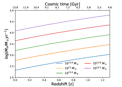
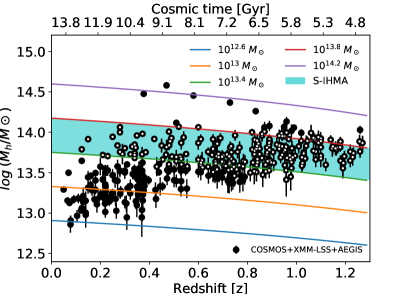
Figure 1: (Upper panel) Mean mass accretion rate of dark matter on to haloes ($\dot{M}_{h}$) as a function of cosmic time and redshift from $z=1.3$ to $z=0$ in Millennium simulations I & II (following equation 2 in Fakhouri et al., 2010). The solid lines show trends for a set of haloes of given masses, $M_{h}=10^{12.6}\;M_{\odot},10^{13}\;M_{\odot},10^{13.4}\;M_{\odot},10^{13.8}\;M_{\odot},10^{14.2}\;M_{\odot}$. (Lower panel) The halo mass of X-ray galaxy groups selected from COSMOS, AEGIS, and XMM-LSS fields as a function of cosmic time (z) (filled and open circles). Solid lines illustrate the redshift evolution of $M_{h}$ for a set of typical haloes with a given initial halo mass (as mentioned in the upper panel) from $z=1.3$ to the present day. In order to investigate the impact of the halo mass growth on the evolution of stellar properties of galaxies such as stellar mass growth, we define a new sample of galaxy groups (open circles) which lie in the highlighted area (S-IHMA).

2 Data of BGGs

2.1 Sample definition and BGG selection

We use galaxy group catalogues, with $M_{h}\sim 5\times 10^{12}$ to $10^{14.5}M_{\odot}$ at $0.04<z<1.9$, which have been selected from the COSMOS (Finoguenov et al., 2007; George et al., 2011), XMM–LSS (Gozaliasl et al., 2014), and AEGIS (Erfanianfar et al., 2013) fields. To ensure the high quality of the photometric redshift of groups, we constrain our study to the redshift range of $0.04<z<1.3$ and study groups with halo mass ranging from $M_{h}\simeq 7.25\times 10^{12}$ to $1.04\times 10^{14}(M_{\odot})$. As in Fig. 1 of paper I (Gozaliasl et al., 2016), we define five subsamples of galaxy groups considering their halo mass-redshift plane as follows:

(S-I) $0.04<$ z $<0.40$ $\&$ $12.85<log(\frac{M_{200}}{M_{\odot}})\leq 13.50$

(S-II) $0.10<$ z $\leq 0.4$ $\&$ $13.50<log(\frac{M_{200}}{M_{\odot}})\leq 14.02$

(S-III) $0.4<$ z $\leq 0.70$ $\&$ $13.50<log(\frac{M_{200}}{M_{\odot}})\leq 14.02$

(S-IV) $0.70<$ z $\leq 1.0$ $\&$ $13.50<log(\frac{M_{200}}{M_{\odot}})\leq 14.02$

(S-V) $1.0<$ z $\leq 1.3$ $\&$ $13.50<log(\frac{M_{200}}{M_{\odot}})\leq 14.02$

Four subsamples (S-II to S-V) cover a similar narrow halo mass range, which allows us to compare the stellar properties of BGGs within haloes of the same masses at different redshifts. The subsample of S-I has a similar redshift range to that of S-II but with a different halo mass range, which enables us to inspect the impact of halo mass on the properties of BGGs at $z<0.4$.

The full details of the sample selection, stellar mass and halo mass measurements have been presented in Gozaliasl et al. (2016) and Gozaliasl et al. (2014). We estimate the halo mass using the $L_{x}-M_{h}$ relation as presented in Leauthaud et al. (2010). We also assume a 0.08 dex extra error in the halo mass estimate in our analysis, which corresponds to a log-normal scatter of the $L_{x}-M_{h}$ relation (Allevato et al., 2012). Table 1 presents the mean stellar mass and halo mass with corresponding statistical and systematic errors for S-I to S-V. The systematic error corresponds to uncertanities in the stellar and halo mass measurements. We note that these systematic errors are taken from the galaxy and group catalogues by Finoguenov et al. (2007); Wuyts et al. (2011); Erfanianfar et al. (2013); Gozaliasl et al. (2014); Laigle et al. (2016).

According to the cold dark matter (CDM) hierarchical structure formation paradigm, dark matter haloes grow by accretion of matter and merging with other (sub)haloes (Frenk et al., 1988). It is well-known that many of the observed galaxy properties correlate with the environment such as the known positive correlation between the stellar mass of the BCGs/BGGs and the halo mass of their host dark matter haloes (Gozaliasl et al., 2016). The slope of this correlation is less than unity, implying that the cluster growth is faster than the BCG growth at the same time. As a result, it is important that the effect of halo growth is taken into account, when galaxy growth is determined. To do this, we use the results presented by Fakhouri et al. (2010) who construct merger trees of dark matter haloes and estimate their merger rates and mass growth rates using the joint data set of the Millennium I and Millennium-II simulations. We use equation 2 by Fakhouri et al. (2010) and determine the mean halo mass growth rates for some typical haloes of given masses ($M_{h}=10^{12.6}\;M_{\odot},10^{13}\;M_{\odot},10^{13.4}\;M_{\odot},10^{13.8}\;M_{\odot},10^{14.2}\;M_{\odot}$) at $z=1.3$. As shown in Fig. 1, the mean mass growth rate slowly decreases with cosmic time for all halo masses. Considering these mass accretion rates, we determine whether $M_{h}$ of these set of haloes grow with cosmic time (z) from $z=1.3$ to the present day (solid lines in the lower panel of Fig. 1).

Following the method used by Groenewald (2016), we construct an evolutionary sequence of galaxy groups at $z<1.3$, then select a new sample of galaxy groups such that their masses lie in the narrow highlighted cyan area and between two halo mass limits (green and red lines), which represent the $M_{h}$ growth for two dark matter haloes with initial masses of $10^{13.4}$ and $10^{13.8}M_{\odot}$ at $z=1.3$, respectively. If a group with $M_{h}\pm 1\sigma$ falls in the highlighted area, it is also included in the sample. We analyse this new sample of groups and the associated BGGs at $0.2<z<1.3$ in §3.3 and compare the results with those for subsamples of S-II to S-V, where the halo mass range is the same for all subsamples and halo mass growth is not taken into account. Hereafter, we will refer to the new Sample with Including Halo Mass Assembly effect as S-IHMA.

We select most of the BGGs from groups by cross-matching their spectroscopic redshifts with the redshift of groups. BGGs with no spectroscopic observations are selected using their photometric redshift (Wuyts et al., 2011; McCracken et al., 2012; Ilbert et al., 2013; Laigle et al., 2016) and the colour-magnitude diagram of group members, as described in detail in Gozaliasl et al. (2014). In this paper, the physical properties of BGGs in the COSMOS field are taken from the COSMOS2015 catalogue (Laigle et al., 2016). This catalogue contains $1,182,103$ objects with a high photometric redshift precision of $\sigma_{\Delta z/(1+z_{sec})}=0.007$ in the 1.5 deg² UltraVISTA-DR2 region. For more detail on the photometric redshift calculation/precision and physical parameter measurement of galaxies, we refer the reader to Laigle et al. (2016).

The sample selection for this work relies on the detection of the outskirts of X-ray galaxy groups. As such, this sample is unbiased towards the presence of the cool cores and therefore the properties of the BCGs. The difference in the completeness are minimized by selecting a relatively narrow range of halo masses for the study. As reported in Tab. 1, the differences ($\lesssim 0.11$ dex) among the mean halo mass of haloes for S-II to S-V lie within the total error.

Table 1: The average systematic error (SYSE) and the statistical error on the mean (SEM) of $log(M_{\star}/M_{\odot})$ and $log(M_{h}/M_{\odot})$ for S-I to S-V. The error values are given in dex.

Sample	$\langle log(M_{\star}/M_{\odot})\rangle$	$dM_{\star}$(SYSE)	$dM_{\star}$(SEM)	$\langle log(M_{h}/M_{\odot})\rangle$	$dM_{h}$(SYSE)	$dM_{h}$(SEM)
S-I	10.84	0.12	0.08	13.28	0.16	0.01
S-II	11.06	0.15	0.07	13.68	0.12	0.02
S-III	11.15	0.16	0.07	13.69	0.15	0.01
S-IV	11.02	0.15	0.05	13.75	0.15	0.01
S-V	10.89	0.19	0.05	13.79	0.16	0.02

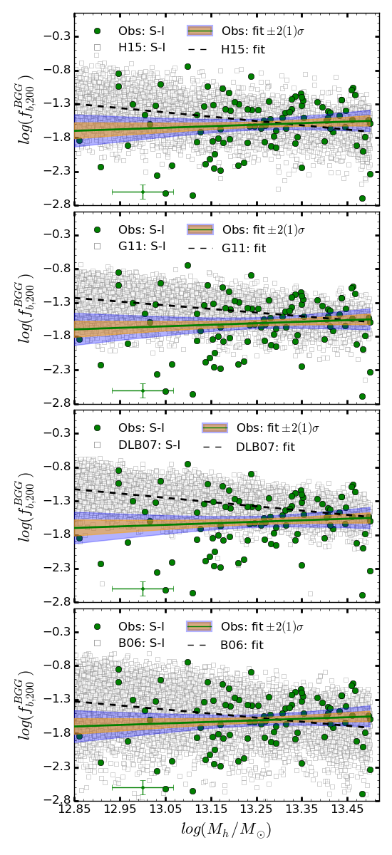
Figure 2: The relative contribution of the stellar populations of the BGGs to the total baryonic mass of hosting groups, $log(f_{200}^{BGG})$, as a function of halo mass ($log(M_{h}/M_{\odot})$). Each row from top to bottom compares the observational data (filled green circles) with the data taken from SAMs of H15, G11, DLB07, and B06 (open gray squares), respectively. The best-fit relation to the data in observations with associated $\pm 1\sigma$ and $\pm 2\sigma$ confidence intervals are shown as the solid green lines and the highlighted orange and blue regions. The best-fit relation for the SAMs are plotted as the dashed black lines. In each plot, we have shown the scale of the median of observed uncertainties on the $log(M_{h}/M_{\odot})$ and $log(f_{200}^{BGG})$ estimates with green error bars.

2.2 Semi-analytic models

We compare our results with a number of theoretical studies, namely with four semi-analytic models (SAMs): Bower et al. (2006) (B06); De Lucia & Blaizot (2007) (DLB07); Guo et al. (2011) (G11); Henriques et al. (2015) (H15). All the models are based on merger trees from the Millennium Simulation (Springel et al., 2005) which provides a description of the evolution of dark matter structures in a cosmological volume. While B06, DLB07 and G11 use the simulation in its original WMAP1 cosmology, H15 scales the merger trees to follow the evolution of large scale structures expressed for the more recent cosmological measurements. With respect to the treatment of baryonic physics, B06 uses the GALFORM version of the Durham model, while DLB07, G11, and H15 follow the Munich L-Galaxies model.

In Gozaliasl et al. (2014), we described some important features of the G11, DLB07, and B06 models. We thus, briefly describe the recent improvements and modifications in the H15 model here and the reader is referred to the Henriques et al. (2015) for further details. With respect to the previous version of L-Galaxies, in addition to the implementation of a PLANCK cosmology, Henriques et al. (2015) uses the Henriques et al. (2013) model for the reincorporation of gas ejected from SN feedback. The scaling of reincorporation time with virial mass, instead of virial velocity, suppresses star-formation in low mass galaxies at earlier times and results in an excellent match between theoretical and observed stellar mass functions at least since $z=3$.

In addition, the H15 model assumes that ram-pressure stripping is only effective in clusters ($M_{vir}>1.2\times 10^{14}\;M_{\odot}$) and has a cold gas surface density threshold for star-formation that is $\sim$ two times smaller than in earlier models. These two modifications ensure that satellite galaxies retain more fuel for star-formation and continue to form stars for longer. This eases a long standing problem with satellite galaxies in theoretical models being quenched too quickly and provides a good match to quenching trends as a function of environment (Henriques et al., 2016). Finally, H15 modified the AGN radio mode accretion rate in order to enhance accretion at $z<0.5$ with respect to earlier times and ensure that galaxies around M* grow significantly down to that redshift, but are predominantly quenched in the local universe.

Table 2: The parameters of the best-fit relation, $log(f_{b,200}^{BGG})=\alpha\times log(M_{200}/M_{\odot})+log(\beta)$, obtained by linear least squares (LLS) and Markov chain Monte Carlo (MCMC) methods for both observations and SAMs. The first column presents the id of subsamples. The second and the third columns list the optimised parameters with 68% confidence intervals by the MCMC method. The fourth and fifth columns present the parameters with $\pm 1\sigma$ error obtained by LLS.

Subsamples	$\alpha_{MCMC}$	$log(\beta_{MCMC})$	$\alpha_{LLS}$	$log(\beta_{LLS})$
S-I
Obs	$+0.209^{+0.166}_{-0.196}$	$-4.393^{+2.598}_{-2.203}$	$+0.228\pm 0.274$	$-4.627\pm 3.624$
H15	$-0.601^{+0.022}_{-0.022}$	$6.412^{+0.288}_{-0.291}$	$-0.6377\pm 0.0215$	$6.890\pm 0.283$
G11	$-0.601^{+0.022}_{-0.021}$	$6.413^{+0.28}_{-0.286}$	$-0.544\pm 0.015$	$5.762\pm 0.190$
DLB07	$-0.603^{+0.014}_{-0.014}$	$6.622^{+0.182}_{-0.184}$	$-0.632\pm 0.014$	$7.00\pm 0.178$
B06	$-0.491^{+0.021}_{-0.021}$	$4.949^{+0.272}_{-0.27}$	$-0.601\pm 0.022$	$6.402\pm 0.283$
S-II
Obs	$-0.573^{+0.289}_{-0.19}$	$6.077^{+2.61}_{-3.944}$	$-0.679\pm 0.338$	$7.520\pm 4.627$
H15	$-0.564^{+0.032}_{-0.033}$	$5.912^{+0.446}_{-0.433}$	$-0.598\pm 0.0328$	$6.389\pm 0.449$
G11	$-0.562^{+0.032}_{-0.033}$	$5.891^{+0.452}_{-0.436}$	$-0.506\pm 0.0359$	$5.247\pm 0.493$
DLB07	$-0.557^{+0.035}_{-0.035}$	$6.006^{+0.481}_{-0.485}$	$-0.573\pm 0.034$	$6.221\pm 0.472$
B06	$-0.495^{+0.057}_{-0.055}$	$4.96^{+0.757}_{-0.779}$	$-0.542\pm 0.057$	$5.610\pm 0.784$
S-III
Obs	$-0.371^{+0.313}_{-0.278}$	$3.361^{+3.792}_{-4.294}$	$-0.493\pm 0.301$	$5.021\pm 4.115$
H15	$-0.625^{+0.028}_{-0.028}$	$6.731^{+0.381}_{-0.382}$	$-0.641\pm 0.028$	$6.943\pm 0.390$
G11	$-0.626^{+0.029}_{-0.029}$	$6.743^{+0.398}_{-0.396}$	$-0.500\pm 0.020$	$5.101\pm 0.269$
DLB07	$-0.563^{+0.019}_{-0.019}$	$6.007^{+0.255}_{-0.258}$	$-0.574\pm 0.019$	$6.153\pm 0.255$
B06	$-0.623^{+0.032}_{-0.032}$	$6.583^{+0.434}_{-0.436}$	$-0.668\pm 0.032$	$7.204\pm 0.433$
S-IV
Obs	$-0.05^{+0.277}_{-0.28}$	$-1.23^{+3.836}_{-3.799}$	$-0.269\pm 0.301$	$1.770\pm 4.255$
H15	$-0.566^{+0.031}_{-0.032}$	$5.925^{+0.434}_{-0.422}$	$-0.585\pm 0.033$	$6.186\pm 0.454$
G11	$-0.57^{+0.032}_{-0.033}$	$5.966^{+0.447}_{-0.437}$	$-0.590\pm 0.030$	$5.164\pm 0.415$
DLB07	$-0.59^{+0.026}_{-0.026}$	$6.321^{+0.36}_{-0.353}$	$-0.600\pm 0.030$	$6.434\pm 0.365$
B06	$-0.67^{+0.048}_{-0.049}$	$7.133^{+0.665}_{-0.652}$	$-0.709\pm 0.048$	$7.669\pm 0.653$
S-V
Obs	$+0.087^{+0.282}_{-0.403}$	$-3.291^{+5.542}_{-3.883}$	$+0.230\pm 0.570$	$-5.252\pm 7.860$
H15	$-0.515^{+0.037}_{-0.038}$	$5.234^{+0.518}_{-0.506}$	$-0.521\pm 0.041$	$5.318\pm 0.554$
G11	$-0.515^{+0.04}_{-0.04}$	$5.239^{+0.541}_{-0.548}$	$-0.499\pm 0.043$	$4.997\pm 0.595$
DLB07	$-0.598^{+0.039}_{-0.04}$	$6.384^{+0.54}_{-0.54}$	$-0.599\pm 0.040$	$6.406\pm 0.541$
B06	$-0.537^{+0.068}_{-0.07}$	$5.232^{+0.951}_{-0.939}$	$-0.578\pm 0.072$	$5.800\pm 0.978$

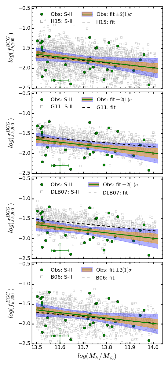
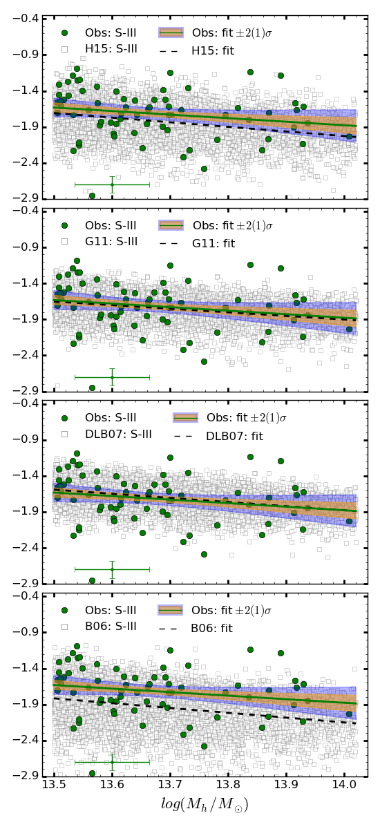
Figure 3: The relative contribution of the BGGs to the total baryonic mass of hosting groups, $log(f_{200}^{BGG})$, as a function of halo mass ($log(M_{h}/M_{\odot})$). Same as in Fig. 2 but for S-II (left column) and S-III (right column), respectively.

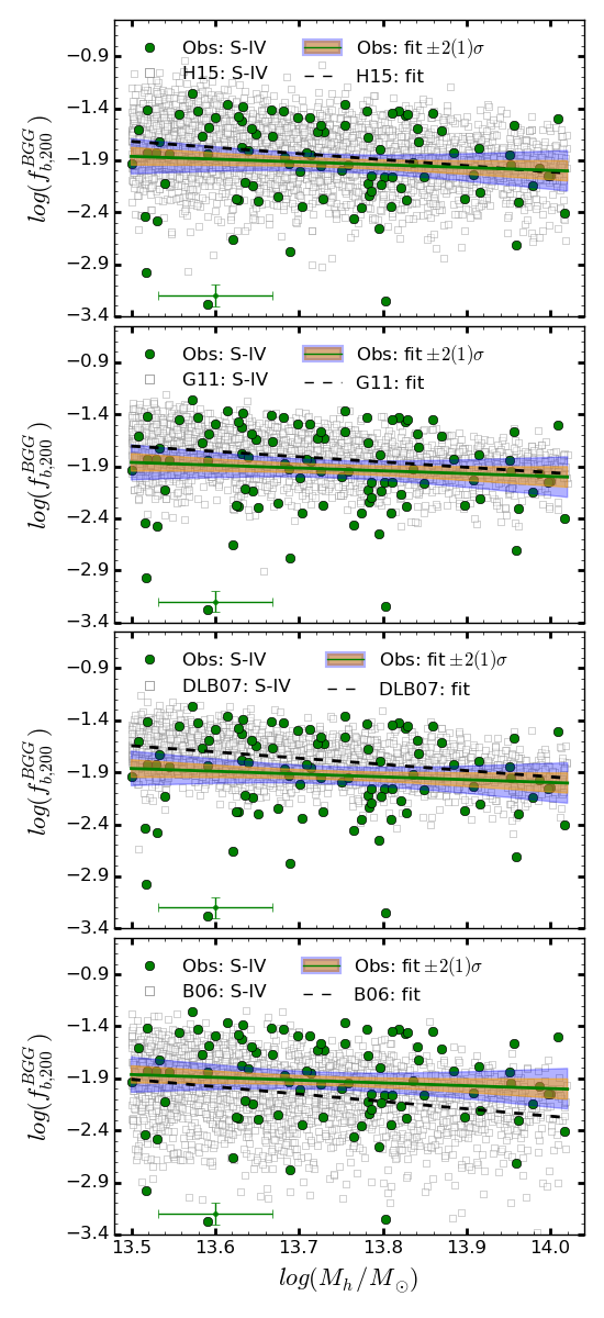
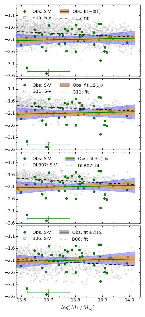
Figure 4: The relative contribution of the BGGs to the total baryonic mass of hosting groups, $log(f_{200}^{BGG})$, as a function of halo mass ($log(M_{h}/M_{\odot})$). The same as in Fig. 2 but for S-IV (left column) and S-V (right column), respectively.

3 Results

3.1 The halo mass dependence of the stellar baryon fractions contained in the BGGs

Galaxy clusters/groups are large enough to represent the mean matter distribution of the Universe (White et al., 1993), thus the ratio of their total baryonic mass (stars, stellar remnants, and gas; $M_{b}$) to their total mass including dark matter ($M_{tot}$) is expected to match the ratio of $\Omega_{b}$ to $\Omega_{m}$ for the universe

$$f_{b}=\frac{M_{b}}{M_{tot}}=\frac{\Omega_{b}}{\Omega_{m}}.$$ (1)

We use cosmological parameters from the full-mission Planck satellite observations of temperature and polarisation anisotropies of the cosmic microwave background radiation (CMB) and Baryon Acoustic Oscillations (BAO) and estimate the observed baryon fraction of the universe ($\Omega_{b}h^{-2}=0.02226\pm 0.00023,\Omega_{m}h^{-2}=0.1415\pm 0.0019$, $f_{b}=0.1573\pm 0.0037$) (Ade et al., 2015) and determine the total baryonic mass of each galaxy group within $R_{200}$ as $M_{b,200}=f_{b}M_{200}$.

In order to quantify the contribution of the BGG stellar component to the total group baryons in observations and SAMs, we estimate the ratio of the stellar mass of BGGs to the total baryonic mass of hosting groups as follows

$$f_{b,200}^{BGG}=\dfrac{M_{\star}^{BGG}}{M_{b,200}}=(\frac{\Omega_{b}}{\Omega_{m}})^{-1}(\frac{M^{BGG}_{*}}{M_{200}}),$$ (2)

where $f_{b,200}^{BGG}$ defines the fraction of the total baryon of a group within $r\sim R_{200}$ contained in stars of the BGG. In §3.1 to 3.2, we only compare our results with predictions from four SAMs (Bower et al., 2006; De Lucia & Blaizot, 2007; Guo et al., 2011; Henriques et al., 2015). The halo mass of groups ($M_{h}$) in all these models correspond to $M_{200c}$, we thus prefer to also use the $M_{200c}$ of groups in observations. However, we convert $M_{200c}$ to $M_{200m}$ in the rest of results presented in §3.4 to 3.6.

In Fig. 2 to 4 , we focus on the halo mass dependency of the $f_{b,200}^{BGG}$. The data associated with the observed sample are shown as filled green circles while the data for the SAMs as shown with open grey squares. Panels from top to bottom compare observations with the SAM of H15, G11, DLB07, and B06, respectively. We approximate the observed and predicted data using a power law relation (e.g., Giodini et al., 2009) given by

$$f_{b,200}^{BGG}=\beta\times(\dfrac{M_{h}}{M_{\odot}})^{\alpha},$$ (3)

where $\alpha$ and $\beta$ present the power low exponent and constant of the $f_{b,200}^{BGG}-M_{h}$ relationship. We take advantage of the properties of logarithms and convert this relation into a linear relationship given by

$$log\;(f_{b,200}^{BGG})=log\;(\beta)+\alpha\times log\;(\dfrac{M_{h}}{{M_{\odot}}}),$$ (4)

we fit this equation to data and quantify the best-fit and optimised parameters by the Linear Least Squares approach and the Markov chain Monte Carlo (MCMC) method in Tab. 2. Since the fitted parameters by two methods are comparable in some cases, we decide to report both parameters in this table. The first column of Tab. 2 presents the subsample ID. The second and third columns present $\alpha_{MCMC}$ and $log\;(\beta_{MCMC})$ with corresponding 68% confidence interval, respectively. The $4^{th}$ and $5^{th}$ columns report $\alpha_{LSS}$ and $log\;(\beta_{LLS})$ with $\pm 1\sigma$ uncertainties, respectively.

In Fig. 2 to 4, the solid green and dashed black lines illustrate the LLS best-fit relations in observations and SAMs, respectively. Our major findings are as follows:

1. For S-I (Fig. 2), we find that $log(f_{b,200}^{BGG})$ shows no significant dependence on $log(M_{h}/M_{\odot})$, while models show that $log(f_{b,200}^{BGG})$ decreases with increasing $log(M_{h}/M_{\odot})$. We note that the best-fit relation to the observational data might be affected due to insufficient number of the low-mass haloes at $log(M_{h}/M_{\odot})<13.15$. Beyond this mass, observations and models become consistent.

2. For S-II (Fig. 3, left), we find that $log(f_{b,200}^{BGG})$ decreases as a function of increasing $log(M_{h}/M_{\odot})$, in a good agreement with all model predictions within $\pm 2\sigma$ errors. Among the models, H15 and B06 are more successful in predicting the observed trend.

3. For S-III (Fig. 3, right), $log(f_{b,200}^{BGG})$ also decreases as a function of increasing $log(M_{h}/M_{\odot})$. The models are consistent with the observed trend within $\pm 2\sigma$ errors. It appears that B06 underestimates $log(f_{b,200}^{BGG})$ at a given halo mass.

4. For S-IV (Fig. 4, left), we find that $log(f_{b,200}^{BGG})$ decreases slowly as a function of increasing $log(M_{h}/M_{\odot})$, in agreement with models within $\pm 2\sigma$ uncertainties.

5. For S-V (Fig. 4, right), we find that $log(f_{b,200}^{BGG})$ increases slowly as a function of increasing $log(M_{h}/M_{\odot})$, which is in contrast with most of the model predictions.

In summary, the observed $log(f_{b,200}^{BGG})$ is found to decrease as a function of increasing $log(M_{h}/M_{\odot})$ a trend which is mildly redshift dependent. The models predict a similar trend but with no significant dependence on redshift.

At $z<0.4$, we find that $log(f_{b,200}^{BGG})$ - $log(M_{h}/M_{\odot})$ relation within haloes with $M_{h}<10^{13.5}\;M_{\odot}$ show an opposite trend compared to the trend within massive haloes.

SAMs generally reproduce the observed $f_{b,200}^{BGG}-M_{200}$ relation of BGGs for S-II to S-V within the uncertainty, however, they fail to adequately predict this relation for S-I.

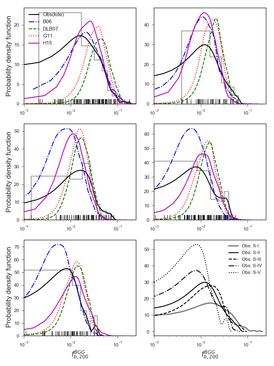
Figure 5: Distribution of $f_{200}^{BGG}$ in observations (solid grey histogram). The smoothed observed distribution (KDE) (solid black line) is compared to those from SAMs of G11 (dotted red line), DLB07 (dashed green line), B06 (dashed-dotted line), and H15 (solid magenta line), respectively. The lower right panel compares the observed KDE functions among S-I to S-V and that of the whole sample of 407 BGGs in observations (solid cyan distribution). The large black ticks (rugs) present the observed one-dimensional density along $f_{200}^{BGG}$-axis.

3.2 Distribution of $f_{b,200}^{BGG}$

In Fig. 5, we present the distribution of $f_{b,200}^{BGG}$ (grey histogram). To compare the observations to models, we use the Kernel Density Estimation (KDE) technique (Rosenblatt, 1956) and determine the smoothed distribution of $f_{b,200}^{BGG}$ in observations (solid black line) and the SAMs of H15 (solid magenta line), G11 (dotted red line), DLB07 ( dashed green line), and B06 (dash-dotted blue line). The y-axes in this distribution display the probability density function and they are normalised in a way that the area under the curves is unity. The lower right panel present the smoothed distribution of $f_{b,200}^{BGG}$ for S-I to S-V and the full sample of BGGs in observations. The rest of panels illustrate the results in observations and models for S-I to S-V, separately. Our main findings in each panel of Fig. 5 are as follows:

1. For S-I, the $f_{b,200}^{BGG}$ distribution spans between $\sim$ 0.002 and 0.18. All SAMs overestimate the position of the centre of the peak (mean value) in the observed distribution. Among them, H15 and B06 predictions are closer to the observations.

2. For S-II, the $f_{b,200}^{BGG}$ distribution extends over 0.004 to 0.06. All the models overestimate the height of the peak. However, H15 and B06 predict correctly the position of the centre of the observed peak.

3. For S-III, the $f_{b,200}^{BGG}$ distribution ranges between 0.001 and 0.08. All models overestimate the height of the peak in the observed distribution. H15 and B06 underestimate the position of the centre of the peak. It appears that models also underestimate the observed probability distribution function at high $f_{b,200}^{BGG}$.

4. The $f_{b,200}^{BGG}$ distribution for S-IV spans between 0.0005 and 0.055. The height of the peak is overestimated by all the models. Among models, H15 better predicts the observations.

5. The $f_{b,200}^{BGG}$ distribution for S-V extends from 0.0003 to 0.037. DLB07, G11, and H15 all over-predict the centre of the peak, while the B06 prediction is in a good agreement with observations.

6. The lower right panel of Fig. 5 compares the smoothed distribution of $f_{b,200}^{BGG}$ in observations for S-I to S-V. We find that the position of the centre of the peak tends to move to lower values with increasing redshift. In addition, we observe that the height of the peak also increases with increasing redshifts of BGGs. The significant changes in the distribution of $f_{b,200}^{BGG}$ occur at $z\sim 0.7$. This comparison shows that $f_{b,200}^{BGG}$ evolves with redshift. As a result, the fraction of BGGs that contribute strongly to the total baryon budget of hosting groups increases with decreasing redshift, suggesting that BGGs may grow considerably in stellar mass at $z<1.3$.

   In addition, we find that the $f_{b,200}^{BGG}$ distribution for S-I skews more to higher values along the x-axes compared to BGGs within massive groups. This indicates that the central galaxies in the low-mass haloes contribute strongly to the total baryonic content of haloes.

3.3 Evolution of SFR, $M_{\star}$, and $f_{b,200}^{BGG}$ of BGGs

In Fig. 5, we find evidence for the redshift evolution of the $f_{b,200}^{BGG}$ distribution. To understand the origin of this evolution, we investigate the stellar mass, SFR, and $log(f_{b,200}^{BGG})$ of the BGGs for S-II to S-V and S-IHMA. We described both data sets in detail in §2.1. We determine the mean and median values of $log(SFR/M_{\odot}yr^{-1})$ (hereafter $log(SFR)$) , $log(M_{\star}/M_{\odot})$ (hereafter $log(M_{\star}$)), and $log(f_{200}^{BGG})$ for S-II to S-V. We also measured these quantities for S-IHMA within 5 redshift bins.

We note that the halo mass growth is taken into account in the sample selection for S-IHMA, while this effect is not considered in the BGG selection for S-II to S-V. The left and right columns of Fig. 6 show results for S-II to S-V and S-IHMA, respectively.

To gain further knowledge on the relative contribution of the BGG stars to the total baryon content of groups, we repeat the same computation for 20% of the BGGs with the highest $f_{200}^{BGG}$ in each redshift bin for both S-II to S-V and S-IHMA, as presented in Fig. 7.

The upper, middle and bottom panels of Fig. 6 and Fig. 7 show the mean and median values of $log(SFR/M_{\odot}yr^{-1})$ (hereafter $log(SFR)$) , $log(M_{\star}/M_{\odot})$ (hereafter $log(M_{\star}$)), and $log(f_{200}^{BGG})$ versus redshift. We describe these relationships in §3.3.1 to §3.3.3, respectively.

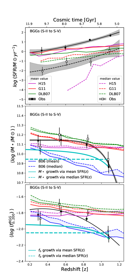
Figure 6: (Upper panels) the mean (median) of $log(SFR/M_{\odot}yr^{-1})$ as a function of redshift for S-II to S-V (left panel) and S-IHMA (right panel). The solid (dashed) black lines show the best-fit function to the mean (median) of $log(SFR/M_{\odot}yr^{-1})$ versus redshift in observations. The mean (median) of $log(SFR/M_{\odot}yr^{-1})-z$ relations in predictions by H15, G11, and DLB07 are shown with solid (dashed) magenta, red, and green lines, respectively. (Middle panels) same as in the upper panel but for $log\;(M_{\star}/M\odot)$ as a function of redshift. We highlight the area between the mean and median trends in model predictions. The cyan solid (dashed) line shows the $M_{\star}$ growths for typical BGGs through the mean (median) SFR-z relations with initial stellar masses which correspond to the mean (median) of stellar mass of BGGs for S-V. (Lower panels) the average/median value of $log(f_{200}^{BGG})$ versus redshift for S-II to S-V (left panel) and S-IHMA (right panel). Same as in the middle panel the shaded regions present the model predictions. The solid (dashed) cyan line shows the growth of $log(f_{200}^{BGG})$ through star-formation for two typical BGGs with initial baryon fractions which correspond to the mean (median) value of $log(f_{200}^{BGG})$ for S-V. Stars in these two typical BGGs are formed in time with mean (median) rate which we approximate in the upper panel.

3.3.1 The SFR evolution of BGGs

In Gozaliasl et al. (2016), we have shown that $\sim 25\%$ and $\sim 60\%$ of the BGGs lie on the main sequence of the star forming galaxies at $0.4<z<0.5$ and $1<z<1.3$, respectively. The SFRs of these galaxies can reach up to $\sim$ 100 $\times$ solar mass per year, in a good agreement with a similar study on 90 BCGs selected from the X-ray galaxy clusters in the 2500-square-degree South Pole Telescope survey by McDonald et al. (2016). They have also found that the SFR of 34% of the BCGs exceeds $10M_{\odot}yr^{-1}$ at $0.25<z<1.25$ and this fraction rises up to $92^{+6}_{-31}$% at $z>1$.

In this paper, we study the redshift evolution of the mean (median) $log(SFR)$ of the BGG to find out what fraction of the $M_{\star}$ and $f^{BGG}_{b,200}$ growth at $z<1.3$ could be driven by the star formation.

The upper panel in Fig. 6 illustrates mean (median) $log(SFR)$ as a function of redshift for BGG within S-II to S-V (left) and BGG within S-IHMA (right). The filled/open black points show the data in the observations. The solid (dashed) green, red, and magenta lines indicate the mean (median) $log(SFR)-z$ relations in the SAMs by DLB07, G11, and H15, respectively. We find that the BGG SFRs in both observations and models follow a bimodal distribution, implying that the mean SFR deviates significantly from the median SFR. In addition, this indicates that BGGs consist of two distinct populations of quiescent and star forming galaxies.

The data in observations shows a rapid evolution at $z>0.7$. This causes the observed trend over $0.1<z<1.3$ to deviate from a linear form. Thus, we use two non-linear relations such as

$$f(z)=\alpha\times z^{\beta}+\gamma,$$ (5)

or the quadratic polynomial

$$f(z)=a+b\times z+c\times z^{2},$$ (6)

to reproduce the trend in the observations. We fit both relation to the data and select the best one. We also note that these best-fit relations may not be valid beyond the redshift range of our BGG sample ($0.1<z<1.3$). The highlighted grey area represents $\pm 1\sigma$ confidence intervals.

Just as in Fig.6, we measure the redshift evolution of mean (median) $log(SFR)$ for 20% of BGGs with the highest $f_{b,200}^{BGG}$ for S-II to S-V and S-IHMA in the upper panel of Fig. 7. Tab. 3 presents the best-fit $log(SFR)-z$ relations.

We summarise the observed and predicted $log(SFR)-z$ relations as follows:

1. The mean (median) $log(SFR)$ of BGGs for both S-II to S-V and S-IHMA decrease considerably with cosmic time by $\sim 2$ dex since $z=1.3$. A significant decline occurs at $z>0.7$. Including the halo mass growth in sample selection has no considerable impact on the evolution of star formation in BGGs at $z<1.3$.

   The mean $log(SFR)$ of 20% of BGGs with the highest $f_{b,200}^{BGG}$ for both S-II to S-V and S-IHMA also decrease in time by $\sim 2$ and $4$ dex since $z=1.3$ to the present day, respectively. It appears that accounting for the halo mass growth in sample selection causes the SFR of BGGs with the highest $f_{b,200}^{BGG}$ to decline more efficiently.

   The median $log(SFR)$ of BGGs (20%) with the highest $f_{b,200}^{BGG}$ show no significant changes with redshift within the uncertainties at $0.2<z<1.2$. The trend for S-IHMA shows a decrease by $\sim$2 dex from z=1.2 to z=0.7 followed by an increase of about 1 dex at low redshifts.

2. All the SAMs consistently predict that mean (median) $log(SFR)$ decreases with redshift by around $0.5-1$ dex. At $z>0.6$, they underestimate the observed mean $log(SFR)$ up to $\sim 1.5$ dex. At lower redshift, their predictions are closer to the observations. The halo mass growth has no considerable effect on the $log(SFR)-z$ relation in model predictions. Except for H15, all the models make a similar prediction for the redshift evolution of the BGG SFR. In the H15 model, the median $log(SFR)$ begins to drop significantly at $z=0.6$. The trends of the mean (median) $log(SFR)-z$ relations in models for the BGGs (20%) with the highest $f_{b,200}^{BGG}$ do not deviate significantly to those of the full BGG sample.

3. In agreement with the models, mean $log(SFR)$ is higher than the median $log(SFR)$ at a given redshift by at least $\sim 1$ dex. This finding shows that BGGs generally consist of two distinct types of galaxies: dead/quiescent objects with no star-formation activity and main-sequence/star-forming galaxies. Thus, the mean SFR of BGGs is influenced by outliers having either very low or very high values of SFRs. It suggests that the mean value of the BGG SFR could not be a typical indicator of star formation activity for all BGGs.

Table 3: We summarise the relation of mean (median) value of $log(SFR/M\odot yr^{-1})$, $log(M\star/M_{\odot}$), and $log(f_{b,200}^{BGG}$) with redshift(z) in observations (as illustrated in Fig. 6 and Fig. 7) using Eq. (5):$f(z)=\alpha\times z^{\beta}+\gamma$ or Eq.(6):$f(z)=a+b\times z+c\times z^{2}$. We have reported the best-fit relations for the full sample of BGGs and 20% of BGGs with the highest f${}_{b,200}^{BGG}$. Since the mean and median values of $log(M\star/M_{\odot}$), and $log(f_{b,200}^{BGG})$ are consistent within errors at fixed redshift, we just present the relation between the mean value of these quantities and redshift. The first column presents the relation and subsample. The columns from 2 to 7 list the best-fit parameters.

Relation (sample)	a	b	c	$\alpha$	$\beta$	$\gamma$
All BGG sample
Mean log(SFR)-z (S-II to S-V)	-2.38 $\pm$ 2.11	0.9 $\pm$ 6.6	1.12 $\pm$ 4.58	-	-	-
Median log(SFR)-z (S-II to S-V)	-0.31 $\pm$ 0.63	0.81 $\pm$ 1.98	0.95 $\pm$ 1.37	-	-	-
Mean log(SFR)-z (S-IHMA)	-	-	-	2.56$\pm$0.56	1.54$\pm$ 0.19	-1.8 $\pm$ 0.16
Median log(SFR)-z (S-IHMA)	-	-	-	1.83$\pm$0.1	1.43$\pm$0.04	0.01$\pm$0.04
20% of BGGs with high $f_{b,200}^{BGG}$
Mean log(SFR)-z (S-II to S-V)	$-1.74\pm 1.7$	$2.96\pm 5.04$	$-0.81\pm 3.26$	-	-	-
Mean log(SFR)-z (S-IHMA)	$-1.23\pm 0.52$	$0.43\pm 1.64$	$1.96\pm 1.15$	-	-	-
All BGG sample
Mean log(M$\star$)-z (S-II to S-V)	-	-	-	7.55 $\pm$ 1.02	-0.14 $\pm$ 0.02	11.14 $\pm$ 0.01
Mean log(M$\star$)-z (S-IHMA)	-	-	-	$1.54\pm 0.19$	$-0.31\pm 0.02$	$11.27\pm 0.02$
20% of BGGs with high $f_{b,200}^{BGG}$
Mean log(M$\star$)-z (S-II to S-V)	11.63 $\pm$ 0.18	-0.37 $\pm$ 0.54	0.19 $\pm$ 0.35	-	-	-
Mean log(M$\star$)-z (S-IHMA)	$11.52\pm 0.23$	$0.59\pm 0.71$	$-0.78\pm 0.5$	-	-	-
All BGG sample
Mean log(f${}_{b,200}^{BGG}$)-z (S-II to S-V)	-1.82 $\pm$ 0.01	0.41 $\pm$ 0.02	-0.61 $\pm$ 0.01	-	-	-
Mean log(f${}_{b,200}^{BGG}$)-z (S-IHMA)	$-1.94\pm 0.08$	$0.68\pm 0.24$	$-0.72\pm 0.16$	-	-	-
20% of BGGs with the highest $f_{b,200}^{BGG}$
Mean log(f${}_{b,200}^{BGG}$)-z (S-II to S-V)	-1.35 $\pm$ 0.14	0.08 $\pm$ 0.41	-0.21$\pm$ 0.27	-	-	-
Mean log(f${}_{b,200}^{BGG}$)-z (S-IHMA)	$-1.68\pm 0.15$	$1.48\pm 0.47$	$-1.38\pm 0.33$	-	-	-

3.3.2 Stellar mass evolution of the BGGs

The hierarchical structure formation theory predicts that the most massive galaxies (e.g., BCGs/BGGs) in the universe should form in the late epochs. In a semi-analytic modelling of galaxy formation based on the Millennium simulation (Springel et al., 2005), De Lucia & Blaizot (2007) found that the BCG mass is assembled relatively late. They obtain 50% of their final mass at z < 0.5 by galactic merging. Using a deep near-IR data of BCGs, (e.g., Collins et al., 2009; Stott et al., 2010) showed that BCGs exhibit little growth in stellar mass at $z<1$. Lidman et al. (2012) studied the correlation between the stellar mass of BCGs and the halo mass of their hosting X-ray clusters and found that the stellar mass of BCGs grows by a factor of 1.8 since $z=0.9$ to $z=0.2$. Such contradictory findings indicate that the detail of the stellar mass growth of BCGs/BGG still remains an unresolved issue in galaxy formation.

In the middle panel of Fig. 6, we determine the mean (median) value of $log(M_{\star})$ as a function of redshift for S-II to S-V (left panel) and S-IHMA (right panel). We do the same computation for the BGGs (20%) with the highest $f_{b,200}^{BGG}$, as shown in the middle panel of Fig. 7.

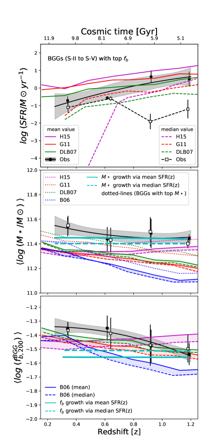
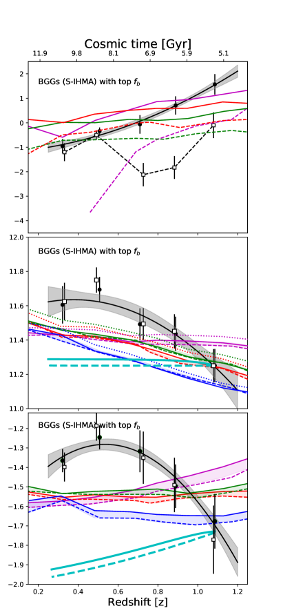
Figure 7: Same as in Fig. 6 but for the 20% of the BGGs with the highest $f_{200}^{BGG}$. In the middle left panel, the dotted magenta, red, green, and blue lines represent the mean stellar mass of 20% of the BGG with highest $M_{\star}$ in the H15, G11, DLB07, and B06 models as a function of redshift.

In the middle panel of Fig. 6, the observed trend indicates that the mean (median) stellar mass of BGGs changes with time in a non-linear fashion (filled/open black points). We fit both non-linear equations of Eq. (5) and (6) to the relation between the mean stellar mass and redshift in observations and choose the best-fit, as presented in Tab. 3. The highlighted gray area illustrates $\pm 1\sigma$ confidence intervals from the fit.

The observed mean $log(SFR)-z$ relation shows that some of BGGs have relatively high-SFRs in particular at $z>0.7$. To quantify a possible contribution of star-formation in the stellar mass growth of BGGs, we assume a typical galaxy with an initial mass which equals the mean (median) stellar mass of BGGs within S-V. We then allow this galaxy to form stars at a rate permitted by the mean (median) $log(SFR)-z$ relations, as approximated in the upper panel of Tab. 3. The solid (dashed) cyan lines represents the $M_{\star}-z$ relation for this typical galaxy.

We summarise our findings in the middle panels of Fig. 7 and Fig. 6 as follows:

1. We find that the mean and median stellar mass of BGGs at a given redshift for observations and model predictions are the same and differences between two quantities lie within the respective errors.

2. The mean (median) stellar mass of BGGs for S-II to S-V and S-IHMA grows as a function of decreasing redshift from z=1.13 (mean (median) redshift of BGGs for S-V) to z=0.31 (mean/median redshift of BGGs for S-II) by $\sim 0.31/0.32$ dex. While the net growth of the BGG stellar mass for S-II to S-V and S-IHMA are similar, however, their trends with redshift differ. The stellar mass of BGGs for S-IHMA changes more linearly with redshift compared to that of S-II to S-V. We note that the significant growth of stellar mass of BGGs for S-II to S-V occurs at $z>0.7$.

3. For 20% of BGGs with the highest $f_{b,200}^{BGG}$ for S-II to S-V, mean (median) $log(M_{\star})$ grows with cosmic time by 0.11 dex, while this growth for S-IHMA is 0.44 dex. This growth is $\sim 0.12$ dex higher than that seen for the full BGG sample, indicating that accounting for the halo growth in the sample selection reveals that BGGs with the highest $f_{b,200}^{BGG}$ assemble more stellar mass by $\sim 0.3$ dex, compared to mass-limited samples (S-II to S-V).

4. In contrast to observations, the mean (median) $M_{\star}$ of BGGs for S-II to S-V and S-IHMA in the G11 and DLB07 SAMs grow slowly in time by about 0.15 dex and 0.25 dex, respectively. The H15 model shows no trend between $M_{\star}$ with redshift. It is also evident that the Munich SAMs (G11, DLB07, and H15) overestimate the stellar mass of BGGs at $z>0.7$. The net growth of $M_{\star}$ for S-II to S-V and S-IHM in the B06 model is much closer to the observed trend compared to the other models. However, this model predicts a linear evolution for the BGG mass and underestimates $M_{\star}$ at intermediate redshifts.

   We find that models underestimate the stellar mass for 20% of BGGs with the highest $f_{b,200}^{BGG}$ for S-II to S-V at a given redshift. For S-IHMA, their predictions are consistent with observations at z=1, but they underpredict the observed stellar mass at lower redshifts. In the middle panel of Fig. 7, we have also shown that the evolution of mean stellar mass for 20% of BGGs with the highest $M_{\star}$ in the SAM predictions by H15, G11, DLB07, and B06 ( dotted magenta, red, green, and blue lines). All the models make predictions which lie under the observed stellar mass.

5. The Munich SAMs overestimate the BGG mass for the full sample of BGGs for S-V at $z>0.8$. On the other hand, they also underestimate the mean SFR of BGGs for S-V. These findings suggest that the star-formation quenching processes in models are more efficient than they needed to be in the early epochs and the BGGs should have possibly grown by non-star forming mechanisms such as dry merger or the tidal striping of stars from satellite galaxies.

6. We find that the mean $log(M_{\star})$ of a typical BGG which obeys the mean $SFR-z$ relation can increase via star-formation by $\sim 0.17$ dex since $z\sim 1.2$, which may explain about 50% of the mean mass growth of a typical star forming BGG at $0.8<z<1.2$. At this period, the stellar mass growth for a typical BGG which follows from the median $SFR-z$ relation is negligible (see solid and dashed cyan lines). The mean (median) stellar mass growth of a typical BGG with the highest $f_{b,200}^{BGG}$ which follows from the mean (median) $SFR-z$ relation for 20% of BGGs with the highest $f_{b,200}^{BGG}$ is also not significant, indicating that BGGs with the highest $f_{b,200}^{BGG}$ grow mainly in stellar mass through dry merging and tidal stripping.

7. In observations, BGGs with the highest $f_{b,200}^{BGG}$ are generally more massive than the BGGs with low $f_{b,200}^{BGG}$ at a fixed redshift by at least 0.25 dex.

3.3.3 The evolution of $f_{200}^{BGG}$

Similarly to computation for the stellar mass of BGGs, we determined the redshift evolution of the mean (median) value of $log(f_{b,200}^{BGG})$ of the full sample of BGGs and 20% of BGGs with the highest $f_{b,200}^{BGG}$ for S-II to S-V (left panel) and S-IHMA (right panel) in the lower panel of Fig. 6 and Fig. 7, respectively.

We quantify what fraction of the growth of $f^{BGG}_{b,200}$ may be driven by star formation in BGGs (solid and dashed cyan lines). We also use Eq. (5) and (6) and summarise the observed trend. The best-fit parameters presented in the lower panel of Tab. 3. We describe the observed and predicted trends as follows:

1. We find that $log(f_{b,200}^{BGG})$ of the entire sample of BGGs for S-II to S-V and S-IHMA increase as a function of decreasing redshift by 0.35 and 0.30 dex since $z\sim 1.13$ (mean/media redshift of BGGs for S-V) to $z\sim 0.31$ (the mean/median redshift of BGGs for S-II). These growths for 20% of the BGGs with the highest $f_{b,200}^{BGG}$ are 0.22 and 0.41 dex, respectively. As a result, the $log(f_{b,200}^{BGG})$ growth of 20% of BGGs with the highest $f_{b,200}^{BGG}$ for S-II to S-V is lower than that of the full sample of BGGs by 0.13 dex. However, this growth for 20% of BGGs with the highest $f_{b,200}^{BGG}$ for S-IHMA is 0.1 dex higher than that of the full sample of BGGs.

2. It is evident that the observed growth in $f_{b,200}^{BGG}$ slows down at $z<0.5$ possibly due to the star-formation quenching in the BGGs and small evolution of the BGG mass.

3. For S-II to S-V, the DLB07 and G11 models predict that the $f_{b,200}^{BGG}$ increases slightly with cosmic time. H15 predicts no $log(f^{BGG}_{b,200})$ growth. The Munich models overestimate the mean (median) of $log(f_{b,200}^{BGG})$ at $z>0.8$. This can be explained by overprediction of the BGG mass at $z>0.8$. Within the models, B06 predictions of the $f_{b,200}^{BGG}$ growth is closer to the observations. However, B06 underestimates $log(f^{BGG}_{b,200})$ at intermediate redshifts. In addition, the Munich models show no significant growth of $f_{b,200}^{BGG}$ for 20% BGGs with the highest $f_{b,200}^{BGG}$. At $z=0.5$, these models underestimate observations.

   For S-IHMA, models estimate a flat trend between $log(f^{BGG}_{b,200})$ and redshift for both the full sample of BGGs and 20% of BGGs with the highest $f_{b,200}^{BGG}$. Within model predictions, B06 predicts $log(f^{BGG}_{b,200})$ to grow a little with redshift. In addition, we observe that accounting for the growth of halo mass in the comparison leads to a 0.1 dex larger increase in $log(f^{BGG}_{b,200})$.

4. We find that $\overline{f_{b,200}^{BGG}}$ of a typical BGG which grows in stellar mass via star-formation (as summarized in Tab. 3) can increase with cosmic time by 0.18 dex (solid cyan line in the lower left panel of Fig. 6) when assuming the halo mass of hosting halo remains constant at $log(M_{200}/M_{\odot})=13.8$ with redshift. In contrast, once we assume this halo to grow in mass according to the rates as illustrated in Fig. 1, the $log(f_{b,200}^{BGG})$ growth via star-formation in the BGG (solid cyan line in the lower right panel of Fig. 6) for S-IHMA becomes less effective at $z\gtrsim 0.8$. At $z\lesssim 0.8$, the halo mass growth rate becomes faster than the SFR. As a result, the growth of $log(f_{b,200}^{BGG})$ at low redshifts can be explained by BGG growth mass through non-star forming process (e.g., dry merger and tidal striping). The $log(f_{b,200}^{BGG})$ growth due to the star-formation is negligible for both the full BGG sample and 20% of the BGGs with the highest $f_{b,200}^{BGG}$.

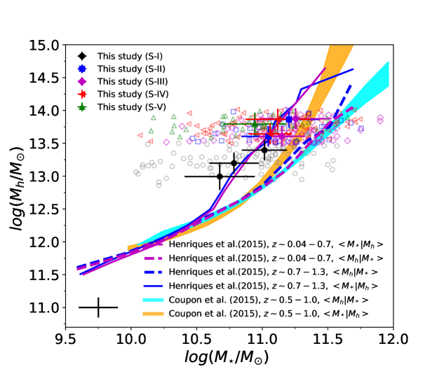
Figure 8: The $M_{\star}-M_{h}$ relation for BGGs in observations, the H15 model, and the result from Coupon et al. (2015). The open symbols show the observed data for S-I to S-V in different color and symbols. The filled data points represent the average $M_{\star}$ of BGGs in our data at fixed halo mass ($\langle M_{\star}|M_{h}\rangle$). The solid magenta and blue lines show $\langle M_{\star}|M_{h}\rangle$ relations in the SAM presented by H15 at $0.04<z<0.7$ and $0.7<z<1.3$ . Similarly, $\langle M_{h}|M_{\star}\rangle$ relations in this model are plotted with dashed blue and magenta lines. The relations from Coupon et al. (2015) results are plotted as orange ($\langle M_{\star}|M_{h}\rangle$) and cyan ($\langle M_{h}|M_{\star}\rangle$) area.

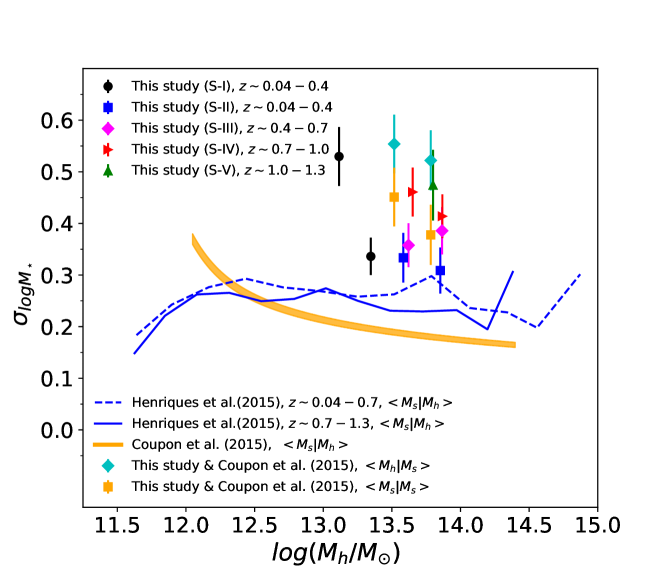
Figure 9: The scatter in the stellar mass of central galaxies ($\sigma_{log\;M_{\star}}$) as a function of halo mass at a fixed halo mass ($\langle M_{\star}|M_{h}\rangle$) in the H15 model at $0.04\leq z\leq 0.7$ (dashed blue line) and $0.7<z\leq 1.3$ (solid blue line). Scatter in $M_{\star}$ at a given halo mass in observations are plotted as the filled black (S-I), blue (S-II), magenta (S-III), red (S-IV), and green (S-V) circles, respectively. The orange area presents $\sigma_{log\;M_{\star}}$ as a function of halo mass from Coupon et al. (2015) results. The cyan diamonds and orange squares represent the scatter between the mean stellar mass of our BGGs and that from $\langle M_{h}|M_{\star}h\rangle$ and $\langle M_{\star}|M_{h}\rangle$ relations presented by Coupon et al. (2015) .

‘

3.4 $M_{*}-M_{h}$ relation and the lognormal scatter in $M_{\star}$ at fixed $M_{h}$ of the BGGs

It is well-known that the stellar mass of central galaxies is correlated with the halo mass and the stellar mass-halo mass relation is a fundamental relationship which is used to link the evolution of galaxies to that of the host haloes. Constraining this relation offers a powerful tool for identifying the role of different physical mechanisms over the evolutionary history of galaxies (Yang et al., 2012; Behroozi et al., 2010b, 2013; Moster et al., 2013; Coupon et al., 2015). Every successful galaxy formation model is expected to make a reasonable prediction of how galaxies grow in mass along with their hosting (sub-)haloes.

The $M_{\star}-M_{h}$ relation can be parametrised in one of the following ways: representing the average stellar mass of BGGs at fixed halo mass or determining the mean halo mass at fixed stellar mass. Hereafter, we will refer to these formalisms as $\langle M_{\star}|M_{h}\rangle$ and $\langle M_{h}|M_{\star}\rangle$, respectively (e.g., Coupon et al., 2015).

Figure 8 shows the $M_{\star}-M_{h}$ relation ($M_{h}$ corresponds to $M_{200m}$, where the mean internal density of the halo is 200 times the mean density of the universe). The halo mass of groups in observations ranges from $10^{12.8}\;M_{\odot}$ to $10^{14}\;M_{\odot}$. Our data also span a wide dynamic range of stellar mass: $10\lesssim log(M_{\star}/M_{\odot})\lesssim 12$. Error bars include both the systematic and statistical errors. We have shown the median error bar on $M_{\star}$ and $M_{h}$ with a black line. In Tab. 1, we have also reported the mean systematic and statistical errors on stellar and halo masses for S-I to S-V. The typical total error on the stellar mass and halo mass in our data correspond to $\sim 0.22$ and $\sim 0.16$ dex, respectively.

In Fig. 8, we have plotted the data for S-I to S-V with open black, blue, magenta, red, and green symbols, respectively. We have also shown the mean stellar mass of BGGs in each subsample with filled symbols. The data show that the stellar mass of BGGs increases as a function of increasing halo mass and more massive haloes host generally more massive central galaxies.

Within four SAMs (G11,DLB07,B06,H15) probed in this paper, we selected the most recently implemented model of H15 and measured both $\langle M_{\star}|M_{h}\rangle$ and $\langle M_{h}|M_{\star}\rangle$ relations over a large range of $M_{h}$ from $10^{11.5};M_{\odot}$ to $10^{14.75}\;M_{\odot}$ at two redshift ranges $0.04<z<0.7$ and $0.7<z<1.3$. As shown in Fig. 8, we find that both $\langle M_{h}|M_{\star}\rangle$ and $\langle M_{\star}|M_{h}\rangle$ show no significant dependence on redshift. Both relations also reveal that $M_{\star}$, similarly, increases with increasing $M_{h}$, however, at $log(M_{h}/M_{\odot})>12.25$, the slope of the $\langle M_{\star}|M_{h}\rangle$ relation becomes steeper than the slope of the $\langle M_{h}|M_{\star}\rangle$ relation and the two trends are separated from each other at higher halo messes. The differences in $M_{\star}$ between $\langle M_{h}|M_{\star}\rangle$ and $\langle M_{\star}|M_{h}\rangle$ relations at a given $M_{h}$ appears to increase as a function of increasing $M_{h}$ by up to 0.5 dex. This means that different type of averaging of halo/stellar mass can highly influence the $M_{\star}-M_{h}$ relation due to the scatter in $M_{\star}$. We find a good agreement between the $\langle M_{\star}|M_{h}\rangle$ relation from the H15 model (solid blue and magenta lines) with our data of BGGs (filled symbols with error bars).

Figure 8 also illustrates the best-fit relation of $\langle M_{\star}|M_{h}\rangle$ (orange area) and $\langle M_{h}|M_{\star}\rangle$ (cyan area) with associated 68% confidence limits for central galaxies at $0.5<z<1.0$ by Coupon et al. (2015). At $log(M_{h}/M_{\odot})<12.75$ and $log(M_{\star}/M_{\odot})<11$, the two relations show similar trends, however, when halo and stellar mass are increased the slope of the $\langle M_{\star}|M_{h}\rangle$ relation becomes steeper than the slope of the $\langle M_{h}|M_{\star}\rangle$ relation and the two trends diverge at $M_{h}=10^{13};M_{\odot}$. The $\langle M_{\star}|M_{h}\rangle$ relation by Coupon et al. (2015) agrees with our observed data within errors. However, the $\langle M_{\star}|M_{h}\rangle$ relation from the H15 model better predicts the observed data compared to the relations of Coupon et al. (2015). The $\langle M_{h}|M_{\star}\rangle$ relation by Coupon et al. (2015) shows a good agreement with that from the H15 model. There is a $\sim 0.4$ dex differences between $M_{\star}$ at a given halo mass between the measurements by Coupon et al. (2015) and H15, which could have arisen from the different methods and quality of data for estimating stellar mass/halo mass estimates and populating haloes by galaxies (such as the difference in the HOD model). We note that the stellar masses in our study are measured by using the Lephare code (Ilbert et al., 2010a) based on the broad band SED fitting technique. Coupon et al. (2015) also use this method. However, we utilize a wealth of multi-wavelength, high signal-to-noise ratio observations such as UltraVISTA survey in the COSMOS field (Laigle et al., 2016) in which the depth of image is higher than data for SPIDER by about $\sim 3$ (AB magnitude) in $K_{s}$ band. Thus, the stellar mass and photometric redshift of galaxies in our sample have been estimated with high accuracy. In addition, using different stellar population models can also bias the stellar mass estimation.

H15 estimated the stellar mass using the Maraston (2005) model as the default stellar population model with a Chabrier (2003) initial mass function (IMF). They have argued that the measurement by Charlot & Bruzual (2007) IMF also gives similar results for all properties of galaxies. However, the measurement with the older model of Bruzual & Charlot (2003) shows some differences in properties of galaxies. Coupon et al. (2015) computed the stellar masses following a procedure reproduced by Arnouts et al. (2013) and use a library of SED templates based on the stellar population synthesis (SPS) code from Bruzual & Charlot (2003) with the Chabrier (2003) IMF. Adopting a different choice of SPS models and IMF can lead to large systematic errors in stellar mass measurements of up to 0.2 dex (Behroozi et al., 2010b; Coupon et al., 2015). In addition, various choice of dust extinction laws can also bias the stellar mass estimates as well. Ilbert et al. (2010b) have estimated a 0.14 dex difference between stellar masses measured with the Calzetti et al. (2000) attenuation law and the Charlot & Fall (2000) dust model. In addition, the assumed cosmology and photometric calibration can also cause further uncertainties in the stellar mass estimates, which are larger than the statistical errors (Coupon et al., 2015).

Observations indicate that galaxy groups can be very diverse in their BGG properties. For example, at fixed group/cluster mass, the $M_{\star}$ of the central galaxies in fossils are larger compared to normal BGGs (e.g., Harrison et al., 2012). Figure 8 shows that $M_{\star}$ at a given $M_{h}$ largely scatters due to the fact that environments have a strong impact on galaxy evolution and every BGG may experience a variety of environmental effects and evolutionary histories.

Models based on the sub-halo abundance matching (SHAM) technique, such as Moster et al. (2013), assume a lognormal scatter in the stellar mass of (central) galaxies at fixed halo mass as $\sigma_{log\;M_{\star}}\sim 0.18$. In Fig. 9, we investigate whether the scatter in the stellar mass of our central galaxies ($\sigma_{log\;M_{\star}}$) changes as a function of halo mass. We compute $\sigma_{log\;M_{\star}}$ for two samples of BGGs selected from the H15 model at $0.04\leq z\leq 0.7$ and $0.7<z\leq 1.3$, as shown with the dashed and solid blue lines, respectively. $\sigma_{log\;M_{\star}}$ corresponds to the standard deviation of stellar mass at a given halo mass. We find that at the halo masses studied here, $\sigma_{log\;M_{\star}}$ exhibits no trend with $M_{h}$ and redshift and it remains constant around $\sigma_{log\;M_{\star}}\sim 0.25$. In addition, we also measure $\sigma_{log\;M_{\star}}$ at fixed halo mass for BGGs in observations. For S-I to S-IV, we determine $\sigma_{log\;M_{\star}}$ in two halo mass bins. For S-I, the stellar mass of BGGs spread over a range characterised by $\sigma_{log\;M_{\star}}=0.5$.

For S-II, we measure a constant scatter for both halo mass bins with $\sigma_{log\;M_{\star}}\sim 0.3$, which is in a good agreement with the prediction of the H15 SAM. We estimate a redshift-dependent scatter for S-III, S-IV as $\sigma_{log\;M_{\star}}\sim 0.35$, $\sigma_{log\;M_{\star}}\sim 0.4$, and $\sigma_{log\;M_{\star}}\sim 0.45$, respectively. It is clearly seen that the scatter in stellar mass of BGGs increases with increasing redshift by $\sim 0.15$ dex between $z\sim 0.1$ and $z\sim 1.3$. In Tab.1, we compare the systematic and statistical errors of the stellar and halo masses, the systematic/statistical errors among different sub-samples (S-I to S-V) and we see a suggestion that the redshift evolution of $\sigma_{log\;M_{\star}}$ might not be due to uncertainties associated to stellar/halo mass measurements. At high redshifts ($z\sim 1$), haloes host a variety of BGG populations in terms of structure, stellar age, and star-formation activities, thus the high scatter in the stellar mass of BGGs at high-z is feasible compared to BGGs at low redshifts, where the majority of them are quiescent elliptical galaxies. In Gozaliasl et al. (2016), we find that the stellar mass distribution of BGGs deviates from a normal/Gaussian distribution with increasing redshift. We find evidence for the presence of a second peak in the stellar mass distribution at lower masses. We suggest that the large scatter in the stellar mass of BGGs in observation is due to their bimodal stellar mass distribution.

The orange area presents the scatter in stellar mass at fixed halo mass from the Coupon et al. (2015) results. Coupon et al. (2015) have presented a parametrised function for $\sigma_{log\;M_{\star}}$ as a function of $M_{\star}$ (see function 9 in Coupon et al. (2015)). Using this function and the $M_{\star}-M_{h}$ relation, we estimate $\sigma_{logM_{\star}}$ as a function of $M_{h}$. $\sigma_{log\;M_{\star}}$ increases with decreasing $M_{h}$, however, at $log(M_{h}/M_{\odot})>12.5$, $\sigma_{logM_{\star}}$ shows no trend with halo mass and remains constant around $\sigma_{log\;M_{\star}}=0.2$. Coupon et al. (2015) report a medium mass ($M_{\star}\sim 10^{10}\;M_{\odot}$) scatter of $\sigma_{log\;M_{\star}}=0.35$ and a high-mass ($M_{\star}\sim 10^{11}\;M_{\odot}$) scatter of $\sigma_{log\;M_{\star}}\simeq 0.2$.

In Fig. 9, to quantify $\sigma_{log\;M_{\star}}$ between the $\langle M_{\star}|M_{h}\rangle$ or $\langle M_{h}|M_{\star}\rangle$ relations from Coupon et al. (2015) results and our data at $0.5<z<1.0$, we follow the procedure that has been presented by Leauthaud et al. (2010) and measure $\sigma_{log\;M_{\star}}$ using the following equation:

$$\sigma_{log\;M_{\star}}=\sqrt{\dfrac{\Delta M_{\star}}{(\gamma-1)}}$$ (7)

where $\Delta M_{\star}$ is the difference of the $log\;M_{\star}$ between our measurement and that from the $\langle M_{\star}|M_{h}\rangle$ or $\langle M_{h}|M_{\star}\rangle$ relations by Coupon et al. (2015). $\gamma-1$ is the slope of halo mass function ($dn/d\;log\;M_{h}\propto M^{-(\gamma-1)}_{h}$). For more details, the reader is referred to Leauthaud et al. (2010).

The filled cyan diamonds and filled orange squares in Fig. 9 illustrate $\sigma_{log\;M_{\star}}$ between the mean stellar mass of our BGGs and those from $\langle M_{h}|M_{\star}\rangle$ and $\langle M_{\star}|M_{h}\rangle$ relations by Coupon et al. (2015), respectively. We find that these dispersions agree with our measurements within errors.

In summary, we conclude that the observed intrinsic lognormal scatter in the stellar mass of BGGs spans a wide range from $\sigma_{log\;M_{\star}}\sim$ 0.25 to 0.5 at $z<1.3$, this holds true over a large range of halo masses. Our measurement is in remarkable agreement with a recent study by Chiu et al. (2016) who estimated the $M_{\star}-M_{h}$ scaling relation for 46 X-ray groups detected in the XMM-Newton-Blanco Cosmology Survey (XMM-BCS) with a halo mass range of $2\times 10^{13} M_{\odot}\leq M_{500}\leq 2.5\times 10^{14}M_{\odot}$(median mass $8\times 10^{13} M_{\odot}$) at redshift $0.1\leq z\leq 1.02$ (median redshift 0.47). They found an intrinsic scatter of $\sigma_{logM_{\star}|M_{500}}=0.36^{+0.07}_{-0.06}$. These scatters that are measured from the observational data are higher than that assumed by theoretical models based on the sub-halo abundance matching (SHAM) technique.

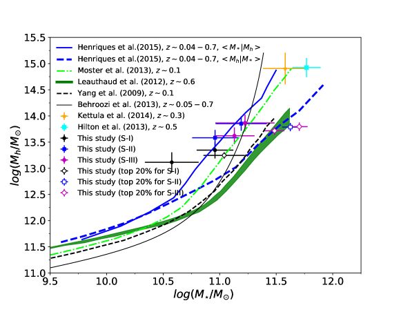
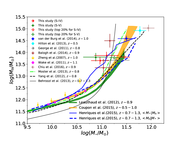
Figure 10: The $M_{\star}-M_{h}$ relation for BGGs/central galaxies compared with a number of results from the literature at similar redshift ranges: $z<0.7$ (upper panel) and $0.7<z<1.3$ (lower panel). The results presented here represent the average stellar mass at fixed halo mass, $\langle M_{\star}|M_{h}\rangle$, but plotted $M_{h}$ as function of $M_{\star}$ to ease the comparison with the literature. The dashed blue line shows the $\langle M_{h}|M_{\star}\rangle$ relation which represents the average halo mass at fixed stellar mass for central galaxies in the H15 model. Following Coupon et al. (2015), the stellar mass of central galaxies in the $M_{\star}-M_{h}$ relation by Leauthaud et al. (2010) (green area) is shifted by 0.2 dex to lower values to compare directly with other results.

3.5 Comparison with the literature

3.5.1 $\langle M_{\star}|M_{h}\rangle$

In Fig 10, we compare the $M_{\star}-M_{h}$ relationship for the BGGs with a number of results from the literature. This relation describes the mean stellar mass at fixed halo mass ($\langle M_{\star}|M_{h}\rangle$), however, to facilitate the comparison with the literature, we plot $M_{h}$ as a function of $M_{\star}$. We have also taken data from Fig. 10 as presented in Coupon et al. (2015) and separately reproduce this figure here at two redshift ranges, $z<0.7$ (upper panel) and $0.7<z<1.3$ (lower panel), respectively.

In the upper panel of Fig. 10, we show $M_{h}$ as a function of $M_{*}$ for S-I, S-II, and S-III, as plotted with filled black, blue and magenta symbols with error bars, respectively. Error bars include both 1$\sigma$ error on the mean value and the error assigned to the stellar/halo mass estimations. We have similarly shown the $M_{h}$ versus $M_{*}$ for the 20% of BGGs with the highest $f_{b,200}^{BGG}$ for S-I to S-III with open black, blue and magenta symbols.

The lower panel of Fig. 10 presents $M_{\star}-M_{h}$ for S-IV (filled red triangles) and S-V (green triangles). We illustrate $M_{h}$ versus $M_{*}$ for the 20% of BGGs with highest $f_{b,200}^{BGG}$ for S-IV and S-V with open red and green symbols. The average stellar mass of BGGs increases with halo mass with a minor dependence on redshift. In both panels of Fig. 10, we find that $M_{\star}$ of the 20% of BGGs with highest $f_{b,200}^{BGG}$ for each subsample are more massive than that of the entire population of BGGs in the same subsample at fixed halo mass.

In both panels of Fig. 10, we show the $M_{h}-M_{*}$ relationship from Behroozi et al. (2013) (solid black line), who constrain it by populating the dark matter haloes from N-body simulation employing the SHAM method and using the observed stellar mass function. They take into account a number of systematic uncertainties such as the errors arising from the choice of cosmology, stellar population synthesis, and IMF, which may affect stellar mass measurements. While this study seems to be consistent with our data at intermediate halo masses, it fails to reproduce the observed results from other studies at high halo masses.

Similarly to Fig. 8, the best-fit $M_{\star}-M_{h}$ relation for the central galaxies with associated $1\sigma$ confidence limits from the Coupon et al. (2015) result is shown as an orange area. This relation is consistent with our observed data within the observational errors.

Figure 10 also shows the results from Leauthaud et al. (2012) (green area) at two redshift ranges $z\sim 0.9$ and $z\sim 0.6$, respectively. Leauthaud et al. (2012) measured the total stellar mass fraction as a function of halo mass at $z=0.2-1.0$ using the HOD model. They also derived the total stellar mass fraction at group scales using the X-ray galaxy groups catalogue in the COSMOS field. Coupon et al. (2015) found a $\sim 0.2$ dex systematic discrepancy between their stellar mass-halo mass scaling relation and that of Leauthaud et al. (2012) at fixed halo mass. This discrepancy is attributed to the differences in the modelling of the HOD, stellar mass measurements and separate choices for the dust extinction law. Coupon et al. (2015) estimated $M_{\star}$ using the SED fitting method similar to the approach presented in Ilbert et al. (2010a) and our study. While Leauthaud et al. (2012) measured $M_{\star}$ with the method described in Bundy et al. (2006). Coupon et al. (2015) compared the stellar mass estimates applying the same IMF and the set of SPS models as Bundy et al. (2006) and Ilbert et al. (2010a) and determined an offset of $\sim 0.2$ dex. Thus they shift the stellar mass-halo mass relation of Leauthaud et al. (2012) to lower values by 0.2 dex along x-axis ($M_{\star}$). Since we have taken the data from Coupon et al. (2015), we applied this shift to the relation by Leauthaud et al. (2012) to lower the stellar mass by 0.2 dex.

Moster et al. (2013), shown as the dot-dashed lime line in Fig. 10, used statistical and SHAM approaches and provided a redshift-dependent parametrisation for the $M_{\star}-M_{h}$ relationship of central galaxies. We find a good agreement between our data and that from Moster et al. (2013).

Figure 10 shows the average stellar mass of BCGs versus the average halo mass for some massive clusters at $z\sim 0.3$ in the CFHTLens field by Kettula et al. (2015) (orange triangle in upper panel). Similarly, Fig. 10 shows the average stellar mass of BCGs versus the average halo mass for clusters at $0.27<z<1.07$ detected using the Atacama Cosmology Telescope, and the Sunyaev-Zeľdovich (SZ) effect by Hilton et al. (2013) (cyan square in both upper and lower panel). The mean stellar mass versus mean halo mass from Chiu et al. (2016) results is shown with a single pink triangle. The halo mass range of these studies are above the halo mass range of our groups.

We show as a single blue diamond the average $M_{h}$ versus mean $M_{\star}$ from van der Burg et al. (2014) in the GCLASS/SpARCS cluster sample at $z\sim 1$, indicating a remarkable agreement with the results of Moster et al. (2013); Coupon et al. (2015); Henriques et al. (2015).

The dashed black line in the upper panel of Fig. 10 presents the $M_{\star}-M_{h}$ relation from the results of Yang et al. (2009), they use the SDSS DR4 catalogue of galaxy groups (Yang et al., 2007) and determine halo mass through an iteratively calculated group luminosity-mass relation. The stellar masses of galaxies were estimated using the relation between $M/L$ and $g-r$ colour assuming a WMAP3 cosmology (Bell, 2003). Yang et al. (2009) is not fully consistent with our data.

The dashed black line in the lower panel of Fig. 10 presents the $M_{\star}-M_{h}$ relation at $z\sim 0.8$ by Yang et al. (2012). This model also overestimates the stellar mass of our BGGs by $0.2$ dex.

The magenta squares with error bars in the lower panel of Fig. 10 illustrate the results from the NEWFIRM Medium-Band Survey at $z\sim 1.1$ by Wake et al. (2011). There is a good agreement between the Wake et al. (2011) results and those from different studies (e.g. Moster et al., 2013; Behroozi et al., 2013; Coupon et al., 2015).

The yellow triangles with error bars present results for the DEEP2, a deep spectroscopic survey with high-density $z\sim 1$ galaxies from the HOD modelling by Zheng et al. (2007), based on real-space clustering and number density measurements.

The grey triangle shows the mean stellar mass of BGGs and the halo mass of their host groups at $0.5<z<1$ in COSMOS field by George et al. (2011). The halo mass of groups has been matched to an X-ray detected sample of groups with the $L_{X}-M_{h}$ relation calibrated weak lensing. The stellar mass has been estimated with an identical method to that of Leauthaud et al. (2012). Our result agree with this study within errors.

The brown triangles represent results from Balogh et al. (2014) with halo mass estimates made using the kinematics of satellites for 11 groups/clusters at $0.8<z<1$ within the COSMOS field.

In the same way as the calculations done in Fig. 8, we show the $\langle M_{\star}|M_{h}\rangle$ (solid blue line) and $\langle M_{h}|M_{\star}\rangle$ (dashed blue line) relations from the SAM of H15 at $z<0.7$ and $0.7\leq z<1.3$ in Fig. 10. The $\langle M_{\star}|M_{h}\rangle$ relation matches remarkably well with observations in both aforementioned redshift ranges.

3.6 $M_{\star}/M_{h}-M_{h}$ relation

As discussed before, the stellar to halo mass ratio ($M_{*}/M_{h}$, SHMR) is one of the key parameter, which provides a powerful insight into the connection between galaxies and their haloes and a useful clue for comprising the integrated efficiency of the past stellar mass assembly (i.e., star-formation and mergers) (e.g. Leauthaud et al., 2012; Coupon et al., 2015; Hudson et al., 2015; Harikane et al., 2016). The studies of low-redshift galaxy systems find a SHMR with a peak at a dark matter halo mass of $M_{h}\sim 10^{12}\;M_{\odot}$, independent of redshift (e.g., Coupon et al., 2015; Hudson et al., 2015; Harikane et al., 2016). However, Leauthaud et al. (2012) claim a redshift evolution of SHMRs from $z\sim 1$ to the present day.

Figure 11 presents the $M_{*}/M_{h}$ as a function of $M_{h}$ for central galaxies at $0.04<z<0.7$ (upper panel) and $0.7<z<1.3$ (lower panel). Just like in Fig. 10, Fig. 11 also compares results from the literature. For further information on the data and studies, we refer the reader to §3.6. We use the same symbols and line styles for the data set used in Fig. 10.

We determine the $M_{\star}/M_{h}-M_{h}$ relation using the H15 model at fixed halo and stellar masses at $0.04<z<0.7$ and $0.7<z<1.3$, as shown in the upper and lower panels of Fig. 11, respectively. At $0.04<z<0.7$, $M_{\star}/M_{h}$ at fixed halo mass (blue solid line) peaks at $log(M_{h}/M_{\odot})=12.08\pm 0.13$ with an amplitude of $0.0200\pm 0.0001$. While $M_{\star}/M_{h}$ at fixed $M_{\star}$ (blue dashed line) reaches its maximum value of $0.0218\pm 0.0003$ at $log(M_{\star}/M_{\odot})=10.93\pm 0.01$, where the average halo mass corresponds to $log(M_{h}/M_{\odot})=12.73\pm 0.01$. In addition, the $M_{\star}/M_{h}-M_{h}$ relation at fixed stellar mass illustrates a flat peak at the halo mass range $log(M_{h}/M_{\odot})=12-13$. At $0.7<z<1.3$, the $M_{\star}/M_{h}$ relation at fixed halo mass (blue solid line) peaks at $log(M_{h}/M_{\odot})=12.09\pm 0.13$ with an amplitude of $0.0181\pm 0.0002$. While this relation at fixed stellar mass (blue dashed line) reaches its maximum value of $0.0202\pm 0.0005$ at $log(M_{\star}/M_{\odot})=10.92\pm 0.09$, where host groups have an average halo mass of $log(M_{h}/M_{\odot})=12.73\pm 0.01$. We find that the $M_{\star}/M_{h}-M_{h}$ relation in the H15 model shows no considerable redshift evolution over $z<1.3$.

In the upper panel of Fig. 11, our data for S-I to S-III show a good agreement with most of the $M_{\star}/M_{h}-M_{h}$ relations presented by Yang et al. (2009); Behroozi et al. (2013); Moster et al. (2013); Henriques et al. (2015). Other observational data from Hilton et al. (2013); Kettula et al. (2015) are also consistent with these theoretical studies at high halo masses. The position and height of the peaks agree with the studies by Yang et al. (2009); Behroozi et al. (2013); Moster et al. (2013). The majority of these studies estimate that $M_{\star}/M_{h}$ reaches its maximum value at around $log(M_{h}/M_{\odot})\sim 11.78-12.3$ with an amplitude of $\sim 0.01-0.02$. Leauthaud et al. (2012) measured the highest peak within studies.

In the lower panel of Fig. 11, we find that our data for S-IV and S-V are also in general agreement with previous studies notably Behroozi et al. (2013); Moster et al. (2013); Coupon et al. (2015); Henriques et al. (2015). There is also a good agreement between other observational results from Zheng et al. (2007); Wake et al. (2011); Hilton et al. (2013); Balogh et al. (2014); van der Burg et al. (2014); Chiu et al. (2016) and theoretical models.

We illustrate $M_{\star}/M_{h}$ versus $M_{h}$ for 20% of the BGGs with the highest $f_{b,200}^{BGG}$ for S-I to S-III (upper panel) and for S-IV and S-V (lower panel) with open symbols. In both panels of Fig 11, we find that $M_{\star}/M_{h}$ for 20% of the BGGs with the highest $f_{b,200}^{BGG}$ for each subsample are higher than that for the full BGG sample at fixed halo mass.

We observe that the scatter in $M_{\star}/M_{h}$ increases towards high halo masses. At $M_{h}=10^{13.8}\;M_{\odot}$, we measure a scatter of $0.003\pm 0.002$ and $0.002\pm 0.001$ in $M_{\star}/M_{h}$ in observations at $0.04<z<0.7$ and $0.7<z<1.3$, respectively. This scatter corresponds to the standard deviation of $M_{\star}/M_{h}$ at fixed halo mass.

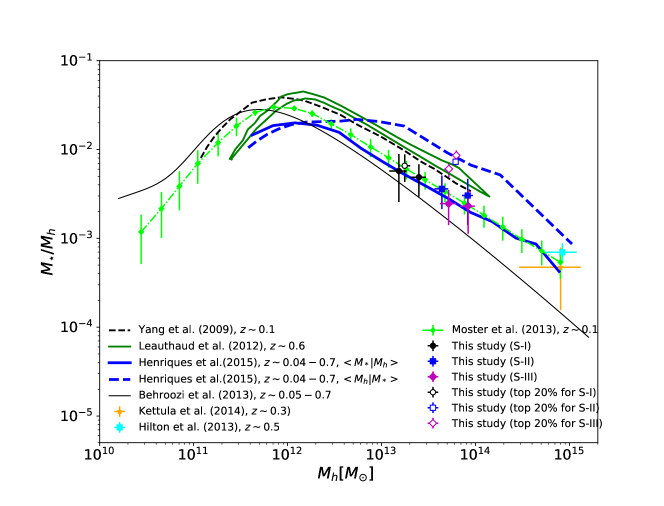
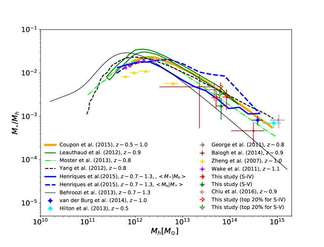
Figure 11: Same data set as used in Fig. 10 but for the stellar to halo mass ratio ($M_{*}/M_{h}$ or SHMR) of BGGs/central galaxies as a function of halo mass at $z<0.7$ (upper panel) and $0.7<z<1.3$ (lower panel).

4 Summary and conclusions

We study the relative contribution of stellar mass of the brightest group galaxies to the total baryonic mass of hosting groups ($f^{BGG}_{b,200}$) and its evolution over $0.04<z<1.3$, using a unique sample of BGGs selected from 407 X-ray galaxy groups in the COSMOS, XMM-LSS and AEGIS fields. We also study the $M_{\star}-M_{h}$ and $M_{\star}/M_{h}-M_{h}$ relations, and quantify the intrinsic (lognormal) scatter in the stellar mass at a fixed halo mass. We define five subsamples of BGGs (S-I to S-V) such that four out of five have similar halo mass range. This definition allows us to compare the properties of the BGGs within haloes of similar masses at different redshifts. In addition, we also selected a new sample of the BGGs accounting for the $M_{h}$ growth of dark matter haloes at $z<1.3$ (S-IHMA). We compare results between these two samples to quantify the impact of the halo mass assembly on the properties of BGGs and their growth over the past 9 billion years. We interpret our results with predictions from four SAMs (H15, G11, DLB07, and B06) based on the Millennium simulation and with a number of results from the literature. We summarize our findings as follows:

1. In agreement with the SAM predictions, the relative contribution of the BGGs to the total baryon content of haloes, $log(f^{BGG}_{b,200})$ decreases with increasing $M_{200}$, at $z<1.0$. While $log(f^{BGG}_{b,200})$ shows no trend with halo mass for the lowest/highest-z BGGs for S-I and S-V. Using the linear least square and MCMC techniques, we quantified the $f^{BGG}_{b,200}-M_{200}$ relations (see Tab. 2) and found that the observed relation evolves mildly with redshift. The slope of the relation becomes steeper with decreasing redshift while the zero-point ($log\beta_{MCMC}$) increases significantly.

2. We obtain an smoothed distribution of the $f^{BGG}_{b,200}$ by applying a non-parametric method to estimate the KDE function. We found that the observed KDE function evolves with redshift and tends be skewn at lower values by increasing redshift. In addition, the smoothed $f^{BGG}_{b,200}$ distribution of the BGGs within $z<0.4$ and low mass group (S-I) skews to higher values compared to that of the BGGs within the same redshift and massive groups (S-II), indicating a high contribution of BGGs to baryons in low-mass haloes. The semi-analytic models probed here are not able to reconstruct the observed $f^{BGG}_{b,200}$ distribution, although H15 and B06 provide, relatively, better predictions.

3. We measured the mean and median SFRs of the BGGs as a function of redshift and found that these quantities decline by $\sim 2$ dex between z=1.2 to z=0.2. As the hierarchical structure formation scenario implies, haloes grow with cosmic time and their abundance with masses $\geq 10^{12}M_{\odot}$ increases (Mo & White, 2002). In this halo mass regime, the influences of environments on galaxy properties within virial radius, heating by virial shocks of infalling gas, energy feedback from an AGN, and gravitational heating of a gas disk by clumpy mass infall, all are efficiently increased (e.g., Lewis et al., 2002; Wetzel et al., 2012). As a result, this makes it likely that the strong evolution of abundance of such massive haloes play a key role in quenching star formation in cluster central galaxies.

   In agreement with observations, SAMs also predict that the observed mean SFR decreases with decreasing redshift by about 1 dex between z=1.2 to z=0.2. However, they underestimate the mean SFR at a given redshift at $z>0.5$. The differences in the mean SFR of BGGs between observations and the models reach up to 1.5 dex at $z=1$. It may be that the BGGs in these models have ended their star-forming activities early.

   We found that the median SFR in the G11 and DLB07 models decreases slowly with cosmic time by $\sim 0.5$ dex from z=1.2 and this trend overcomes observations at $z<0.8$. The median SFR predicted by H15 model decreases sharply by $\geq 4$ dex and this model underestimates significantly SFRs in particular at low redshifts.

   In agreement with the models, we find no considerable differences among the mean (median) SFR of the full BGG sample between S-II to S-V and S-IHMA. This indicates that accounting for the growth of halo mass in the comparison leads to no significant changes in the SFR evolution.

   The mean SFR of 20% of the BGGs with the highest $f^{BGG}_{b,200}$ for both S-II to S-V and S-IHMA decrease as a function of decreasing redshift by $\sim 2$ dex and $\sim 3$ dex, respectively. The trend for S-II to S-V is slower than that of S-IHMA at $z>0.6$. Models predict better evolution the mean (median) SFR of the 20% of BGGs for S-II to S-V and S-IHMA than SFR of the full BGG sample.

   We found that the BGG SFR exhibits a bimodal distribution. As a result, the mean SFR is $\sim 2$ dex higher than the median SFR at fixed redshift. Such a large gap indicates that the mean SFR of BGGs is influenced by outliers (very high and low SFRs). We suggest that BGGs consist of two distinct populations of star-forming and passive galaxies.

4. We determined that the stellar mass of BGGs for both S-II to S-V and S-IHMA grows as a function of decreasing redshift by at least 0.3 dex. While the significant growth for S-II to S-V occurs at $z>0.7$ and slows down at low redshifts, the stellar mass for S-IHMA linearly increases with redshift from z=1.2 to the present day.

   The mean (median) stellar mass of the 20% of BGGs with the highest $f^{BGG}_{b,200}$ for S-II to S-V and S-IHMA increases by 0.11 dex and 0.44 dex over $0.31<z<1.13$. The stellar mass growth for S-IHMA is substantially higher than that of S-II to S-V by 0.33 dex, illustrating that the halo mass growth results in BGGs with the highest $f^{BGG}_{b,200}$ to grow further. We found that 20% of the BGGs with the highest $f^{BGG}_{b,200}$ are generally more massive galaxies compared to BGGs with low $f^{BGG}_{b,200}$ by at least 0.2 dex at a given redshift.

   We show that 45% of the growth of stellar mass for a typical star forming BGG which follow the mean $SFR-z$ relation (as presented in Tab. 3) could be driven by star-formation since $z<1.3$. However, this growth for a typical BGG which follows the median $SFR-z$ relation is not significant.

   Munich models are found to underestimate the stellar mass growth of BGGs at $z<1.3$. They also overestimate the stellar mass of BGGs at $z>1.0$. This can be explained to be due to overestimating the number density of massive galaxies and the number of major mergers that BGGs may have experienced at high-z. For the 20% BGGs with highest $f_{b,200}^{BGG}$, models underestimate the BGGs mass, particularly at intermediate redshifts. We quantified the growth of the mean $M_{\star}$ for the 20% BGGs with the highest $M_{\star}$, with redshift, in models and showed that their trends approach the observed trend, however, their predictions are still below observations by $1\sigma$.

5. We investigated the mean (median) $log(f_{b,200}^{BGG})-z$ relation of the BGGs and found that $log(f_{b,200}^{BGG})$ increases with decreasing redshift from $z=1.13$ to $z=0.31$ by $0.33-0.35$ dex. Munich models (H15, G11, and DLB07) predict no significant growth for $log(f_{b,200}^{BGG})$ with redshift and overpredict the $f_{b,200}^{BGG}$ at $z>0.8$. Since models under-predict the SFR at $z>0.8$, we conclude that these models possibly overestimate either the number of early major mergers or early SFRs of the BGGs.

   The $log(f_{b,200}^{BGG})$ for the 20% BGGs with the highest $f_{b,200}^{BGG}$ for S-II to S-V and S-IHMA increases with cosmic time by $0.22$ and $0.41$ dex, indicating that the halo mass growth is efficient in the $log(f_{b,200}^{BGG})$ growth. SAMs match data for S-II to S-V better than those of S-IHMA.

   We quantified what fraction of the $f_{b,200}^{BGG}$ growth for a typical galaxy may have been driven by star formation in the BGGs. We assume a typical galaxy with an initial mass which corresponds to the mean (median) stellar mass of BGGs for S-V. We allowed this galaxy to form stars according to the mean (median) SFR-z trends as summarised in Tab. 3. We also measured the halo mass growth for the hosting group with initial mass which is equal to the mean (median) halo mass of groups for S-V. When the halo mass of a typical halo remains constant with redshift, $f_{b,200}^{BGG}$ of the typical star forming BGG can increase via star formation by 0.18 dex over $z<1.3$. In contrast, once we allow the halo to grow in mass with redshift, the $f_{b,200}^{BGG}$ growth via star formation becomes negligible at $z<0.8$, indicating that the halo mass growth rate is more efficient than the star formation rate.

   In addition, $f_{b,200}^{BGG}$ which follows the median SFR-z relation indicates no growth through star-formation for both the entire sample of the BGGs and the 20% BGGs with the highest $f_{b,200}^{BGG}$.

6. We found no strong correlation between the $f^{BGG}_{b,200}$ and the evolutionary state of the groups, probed by the luminosity gap in the r-band magnitude between the BGG and the second brightest satellite ($r\simeq 0.052$).

7. The observed $M_{\star}/M_{h}-M_{h}$ and $M_{\star}-M_{h}$ relations are generally consistent with the SAM predictions. However, there are some discrepancies at low and high halo masses which can depend on the statistical methods used for the comparison. As an example, we obtained both $\langle M_{\star}|M_{h}\rangle$ and $\langle M_{h}|M_{\star}\rangle$ relations for the H15 model and found that the slope of the $\langle M_{\star}|M_{h}\rangle$ relation becomes steeper than that of $\langle M_{h}|M_{\star}\rangle$ relation at $M_{h}>10^{12.5}\;M_{\odot}$.

8. By comparing a number of $M_{\star}-M_{h}$ relations from the literature, we showed that the scatter in stellar mass of BGGs ($\sigma_{log\;M_{\star}}$) at a given halo mass is one of the key issues which leads to inconsistencies between results.

   Using the H15 model, we find that $M_{\star}-M_{h}$, and $\sigma_{log\;M_{\star}}-M_{h}$ relations show no evolution since $z\sim 1$ and $\sigma_{log\;M_{\star}}$ also shows no trend with $M_{h}$ at halo mass $M_{h}=10^{12}$ to $10^{14.5}M_{\odot}$. The scatter in the stellar mass of BGGs is found to remain constant at around $\sigma_{log\;M_{\star}}\sim 0.25$.

   The scatter in $M_{\star}$ of BGGs in observations is relatively higher than the model predictions and $\sigma_{log\;M_{\star}}$ increases when increasing redshift from $\sigma_{log\;M_{\star}}\sim 0.3$ at $z\sim 0.2$ to $\sigma_{log\;M_{\star}}\sim 0.5$ at $z\sim 1.0$. Our findings are in remarkable agreement with the recent research by Chiu et al. (2016) who estimated the $M_{\star}-M_{h}$ scaling relation for 46 X-ray groups detected in the XMM-Newton-Blanco Cosmology Survey (XMM-BCS) with a median halo mass of $8\times 10^{13} M_{\odot}$ at a median redshift of $z=0.47$. This study measured an intrinsic scatter in stellar mass of BGGs by $\sigma_{logM_{\star}|M_{500}}=0.36^{+0.07}_{-0.06}$. In Gozaliasl et al. (2016), we have found evidence for the presence of a second peak in the $M_{\star}$ distribution of BGGs around $M_{\star}\sim 10^{10.5}\;M_{\odot}$ and showed that the shape of $M_{\star}$ distribution deviates from a normal distribution when increasing redshift. As a result, the BGGs that make the second peak are found to be generally young and star forming systems, implying that the presence of high scatter in the $M_{\star}-M_{h}$ relation is a feasible effect due to the presence of BGGs with a variety of properties e.g., star formation and stellar age.

9. The $M_{\star}/M_{h}-M_{h}$ relation which we measure using the H15 model peaks at $log(M_{h}/M_{\odot})=12.08\pm 0.13$ with an amplitude of $0.0200\pm 0.0001$ at $0.04<z<0.7$ and $0.0181\pm 0.0002$ at $0.7<z<1.3$, which is roughly independent of redshift.

   At $M_{h}=10^{13.8}\;M_{\odot}$, $M_{*}/M_{h}$ in observations scatters by $0.003\pm 0.002$ with no dependence on redshift.

10. We point out that the different choices of the statistical analysis, data fitting techniques, and the ravaging methods, altogether, can cause bias results. It is advantageous to distinguish the results which are derived for the mean and median values of the BGG properties. Classification of BGGs based on their SFR/stellar age can obviously provide more insight onto some of the hidden properties of BGGs.

11. We have compared observed trends with SAMs based on the Millennium Simulation and explored that the models are generally able to predict observational results. However, in order to advance our understanding of galaxy formation further, a grid of model predictions fully sampling the parameter space of amplitude and redshift evolution of the relevant physical processes such as star formation and AGN feedback is necessary.

5 Acknowledgements

This work has been supported by the grant from the Finnish Academy of Science to the University of Helsinki and the Euclid project, decision numbers 266918 and 1295113. The first author wishes to thank Donald Smart and Christopher Haines for the useful comments and the School of Astronomy in Institute for Research in Fundamental Sciences for its support. We used the data of the Millennium simulation and the web application providing on-line access to them were constructed as the activities of the German Astrophysics Virtual Observatory.

References

- Ade et al. (2015) Ade P., Aghanim N., Arnaud M., Ashdown M., Aumont J., Baccigalupi C., Banday A., Barreiro R., Bartlett J., Bartolo N., et al., 2015, arXiv preprint arXiv:1502.01591
- Allen et al. (2008) Allen S., Rapetti D., Schmidt R., Ebeling H., Morris R., Fabian A., 2008, MNRAS, 383, 879
- Allen et al. (2004) Allen S., Schmidt R., Ebeling H., Fabian A., Van Speybroeck L., 2004, MNRAS, 353, 457
- Allen et al. (2011) Allen S. W., Evrard A. E., Mantz A. B., 2011, arXiv preprint arXiv:1103.4829
- Allevato et al. (2012) Allevato V., Finoguenov A., Hasinger G., Miyaji T., Cappelluti N., Salvato M., Zamorani G., Gilli R., George M., Tanaka M., et al., 2012, The Astrophysical Journal, 758, 47
- Andreon (2010) Andreon S., 2010, MNRAS, 407, 263
- Arnouts et al. (2013) Arnouts S., Le Floc’h E., Chevallard J., Johnson B. D., Ilbert O., Treyer M., Aussel H., Capak P., Sanders D. B., Scoville N., McCracken H. J., Milliard B., Pozzetti L., Salvato M., 2013, A&A, 558, A67
- Balogh et al. (2014) Balogh M. L., McGee S. L., Mok A., Wilman D. J., Finoguenov A., Bower R. G., Mulchaey J. S., Parker L. C., Tanaka M., 2014, MNRAS, 443, 2679
- Behroozi et al. (2010a) Behroozi P. S., Conroy C., Wechsler R. H., 2010a, The Astrophysical Journal, 717, 379
- Behroozi et al. (2010b) Behroozi P. S., Conroy C., Wechsler R. H., 2010b, ApJ, 717, 379
- Behroozi et al. (2013) Behroozi P. S., Wechsler R. H., Conroy C., 2013, ApJ, 770, 57
- Bell (2003) Bell E. F., 2003, The Astrophysical Journal, 586, 794
- Berlind & Weinberg (2002) Berlind A. A., Weinberg D. H., 2002, The Astrophysical Journal, 575, 587
- Bower et al. (2006) Bower R., Benson A., Malbon R., Helly J., Frenk C., Baugh C., Cole S., Lacey C. G., 2006, MNRAS, 370, 645
- Bruzual & Charlot (2003) Bruzual G., Charlot S., 2003, MNRAS, 344, 1000
- Bulbul et al. (2016) Bulbul E., Randall S. W., Bayliss M., Miller E., Andrade-Santos F., Johnson R., Bautz M., Blanton E. L., Forman W. R., Jones C., et al., 2016, ApJ, 818, 131
- Bundy et al. (2006) Bundy K., Ellis R. S., Conselice C. J., Taylor J. E., Cooper M. C., Willmer C. N., Weiner B. J., Coil A. L., Noeske K. G., Eisenhardt P. R., 2006, The Astrophysical Journal, 651, 120
- Calzetti et al. (2000) Calzetti D., Armus L., Bohlin R. C., Kinney A. L., Koornneef J., Storchi-Bergmann T., 2000, The Astrophysical Journal, 533, 682
- Chabrier (2003) Chabrier G., 2003, Publications of the Astronomical Society of the Pacific, 115, 763
- Charlot & Bruzual (2007) Charlot S., Bruzual G., 2007, provided to the community but not published
- Charlot & Fall (2000) Charlot S., Fall S. M., 2000, The Astrophysical Journal, 539, 718
- Chiu et al. (2016) Chiu I., Mohr J., McDonald M., Bocquet S., Ashby M., Bayliss M., Benson B., Bleem L., Brodwin M., Desai S., et al., 2016, MNRAS, 455, 258
- Chiu et al. (2016) Chiu I., Saro A., Mohr J., Desai S., Bocquet S., Capasso R., Gangkofner C., Gupta N., Liu J., 2016, Monthly Notices of the Royal Astronomical Society, 458, 379
- Collins et al. (2009) Collins C. A., Stott J. P., Hilton M., Kay S. T., Stanford S. A., Davidson M., Hosmer M., Hoyle B., Liddle A., Lloyd-Davies E., Mann R. G., Mehrtens N., Miller C. J., Nichol R. C., Romer A. K., Sahlén M., Viana P. T. P., West M. J., 2009, Nature, 458, 603
- Coupon et al. (2015) Coupon J., Arnouts S., van Waerbeke L., Moutard T., Ilbert O., van Uitert E., Erben T., Garilli B., Guzzo L., Heymans C., et al., 2015, MNRAS, 449, 1352
- David et al. (1995) David L. P., Jones C., Forman W., 1995, ApJ, 445, 578
- De Lucia & Blaizot (2007) De Lucia G., Blaizot J., 2007, MNRAS, 375, 2
- Dunkley et al. (2009) Dunkley J., Komatsu E., Nolta M., Spergel D., Larson D., Hinshaw G., Page L., Bennett C., Gold B., Jarosik N., et al., 2009, The Astrophysical Journal Supplement Series, 180, 306
- Dvorkin & Rephaeli (2015) Dvorkin I., Rephaeli Y., 2015, MNRAS, 450, 896
- Erfanianfar et al. (2013) Erfanianfar G., Finoguenov A., Tanaka M., Lerchster M., Nandra K., Laird E., Connelly J., Bielby R., Mirkazemi M., Faber S., et al., 2013, ApJ, 765, 117
- Ettori et al. (2009) Ettori S., Morandi A., Tozzi P., Balestra I., Borgani S., Rosati P., Lovisari L., Terenziani F., 2009, A&A, 501, 61
- Evrard (1997) Evrard A. E., 1997, MNRAS, 292, 289
- Fakhouri et al. (2010) Fakhouri O., Ma C.-P., Boylan-Kolchin M., 2010, Monthly Notices of the Royal Astronomical Society, 406, 2267
- Finoguenov et al. (2007) Finoguenov A., Guzzo L., Hasinger G., Scoville N., Aussel H., Böhringer H., Brusa M., Capak P., Cappelluti N., Comastri A., et al., 2007, ApJS, 172, 182
- Frenk et al. (1988) Frenk C. S., White S. D., Davis M., Efstathiou G., 1988, The Astrophysical Journal, 327, 507
- George et al. (2011) George M. R., Leauthaud A., Bundy K., Finoguenov A., Tinker J., Lin Y.-T., Mei S., Kneib J.-P., Aussel H., Behroozi P. S., et al., 2011, ApJ, 742, 125
- Giodini et al. (2012) Giodini S., Finoguenov A., Pierini D., Zamorani G., Ilbert O., Lilly S., Peng Y., Scoville N., Tanaka M., 2012, Astronomy & Astrophysics, 538, A104
- Giodini et al. (2009) Giodini S., Pierini D., Finoguenov A., Pratt G., Boehringer H., Leauthaud A., Guzzo L., Aussel H., Bolzonella M., Capak P., et al., 2009, ApJ, 703, 982
- Gonzalez et al. (2013) Gonzalez A. H., Sivanandam S., Zabludoff A. I., Zaritsky D., 2013, ApJ, 778, 14
- Gozaliasl et al. (2014) Gozaliasl G., Finoguenov A., Khosroshahi H., Mirkazemi M., Salvato M., Jassur D., Erfanianfar G., Popesso P., Tanaka M., Lerchster M., et al., 2014, A&A, 566, A140
- Gozaliasl et al. (2016) Gozaliasl G., Finoguenov A., Khosroshahi H. G., Mirkazemi M., Erfanianfar G., Tanaka M., 2016, Monthly Notices of the Royal Astronomical Society, 458, 2762
- Gozaliasl et al. (2014) Gozaliasl G., Khosroshahi H., Dariush A., Finoguenov A., Jassur D., Molaeinezhad A., 2014, A&A, 571, A49
- Groenewald (2016) Groenewald D. N., 2016, PhD thesis, North-West University (South Africa), Potchefstroom Campus
- Guo et al. (2011) Guo Q., White S., Boylan-Kolchin M., De Lucia G., Kauffmann G., Lemson G., Li C., Springel V., Weinmann S., 2011, MNRAS, 413, 101
- Harikane et al. (2016) Harikane Y., Ouchi M., Ono Y., More S., Saito S., Lin Y.-T., Coupon J., Shimasaku K., Shibuya T., Price P. A., et al., 2016, The Astrophysical Journal, 821, 123
- Harrison et al. (2012) Harrison C. D., Miller C. J., Richards J. W., Lloyd-Davies E., Hoyle B., Romer A. K., Mehrtens N., Hilton M., Stott J. P., Capozzi D., et al., 2012, The Astrophysical Journal, 752, 12
- Henriques et al. (2016) Henriques B., White S. D., Thomas P. A., Angulo R. E., Guo Q., Lemson G., Wang W., 2016, arXiv preprint arXiv:1611.02286
- Henriques et al. (2015) Henriques B. M., White S. D., Thomas P. A., Angulo R., Guo Q., Lemson G., Springel V., Overzier R., 2015, MNRAS, 451, 2663
- Henriques et al. (2013) Henriques B. M., White S. D., Thomas P. A., Angulo R. E., Guo Q., Lemson G., Springel V., 2013, Monthly Notices of the Royal Astronomical Society, 431, 3373
- Hilton et al. (2013) Hilton M., Hasselfield M., Sifón C., Baker A. J., Barrientos L. F., Battaglia N., Bond J. R., Crichton D., Das S., Devlin M. J., et al., 2013, MNRAS, p. stt1535
- Hudson et al. (2015) Hudson M. J., Gillis B. R., Coupon J., Hildebrandt H., Erben T., Heymans C., Hoekstra H., Kitching T. D., Mellier Y., Miller L., et al., 2015, Monthly Notices of the Royal Astronomical Society, 447, 298
- Ilbert et al. (2013) Ilbert O., McCracken H., Le Fèvre O., Capak P., Dunlop J., Karim A., Renzini M., Caputi K., Boissier S., Arnouts S., et al., 2013, A&A, 556, A55
- Ilbert et al. (2010b) Ilbert O., Salvato M., Le Floc’h E., Aussel H., Capak P., McCracken H., Mobasher B., Kartaltepe J., Scoville N., Sanders D., et al., 2010b, The Astrophysical Journal, 709, 644
- Ilbert et al. (2010a) Ilbert O., Salvato M., Le Floc’h E., Aussel H., Capak P., McCracken H., Mobasher B., Kartaltepe J., Scoville N., Sanders D., et al., 2010a, ApJ, 709, 644
- Kettula et al. (2015) Kettula K., Giodini S., Van Uitert E., Hoekstra H., Finoguenov A., Lerchster M., Erben T., Heymans C., Hildebrandt H., Kitching T., et al., 2015, MNRAS, 451, 5978
- Khosroshahi et al. (2007) Khosroshahi H. G., Ponman T. J., Jones L. R., 2007, Monthly Notices of the Royal Astronomical Society, 377, 595
- Kravtsov et al. (2004) Kravtsov A. V., Berlind A. A., Wechsler R. H., Klypin A. A., Gottlöber S., Allgood B., Primack J. R., 2004, The Astrophysical Journal, 609, 35
- Laigle et al. (2016) Laigle C., Capak P., Scoville N., 2016, Astrophysical Journal Supplement Series, 224, Art
- Leauthaud et al. (2010) Leauthaud A., Finoguenov A., Kneib J.-P., Taylor J. E., Massey R., Rhodes J., Ilbert O., Bundy K., Tinker J., George M. R., et al., 2010, The Astrophysical Journal, 709, 97
- Leauthaud et al. (2012) Leauthaud A., George M. R., Behroozi P. S., Bundy K., Tinker J., Wechsler R. H., Conroy C., Finoguenov A., Tanaka M., 2012, ApJ, 746, 95
- Lewis et al. (2002) Lewis I., Balogh M., De Propris R., Couch W., Bower R., Offer A., Bland-Hawthorn J., Baldry I. K., Baugh C., Bridges T., et al., 2002, Monthly Notices of the Royal Astronomical Society, 334, 673
- Lidman et al. (2012) Lidman C., Suherli J., Muzzin A., Wilson G., Demarco R., Brough S., Rettura A., Cox J., DeGroot A., Yee H. K. C., Gilbank D., Hoekstra H., Balogh M., Ellingson E., Hicks A., Nantais J., Noble A., Lacy M., Surace J., Webb T., 2012, MNRAS, 427, 550
- Lin et al. (2003) Lin Y.-T., Mohr J. J., Stanford S. A., 2003, ApJ, 591, 749
- McCarthy et al. (2007) McCarthy I. G., Bower R. G., Balogh M. L., 2007, MNRAS, 377, 1457
- McCarthy et al. (2010) McCarthy I. G., Schaye J., Ponman T. J., Bower R. G., Booth C. M., Dalla Vecchia C., Crain R. A., Springel V., Theuns T., Wiersma R. P., 2010, Monthly Notices of the Royal Astronomical Society, 406, 822
- McCracken et al. (2012) McCracken H., Milvang-Jensen B., Dunlop J., Franx M., Fynbo J., Le Fèvre O., Holt J., Caputi K., Goranova Y., Buitrago F., et al., 2012, A&A, 544, A156
- McDonald et al. (2016) McDonald M., Stalder B., Bayliss M., Allen S., Applegate D., Ashby M., Bautz M., Benson B., Bleem L., Brodwin M., et al., 2016, The Astrophysical Journal, 817, 86
- McGaugh et al. (2009) McGaugh S. S., Schombert J. M., De Blok W., Zagursky M. J., 2009, ApJ, 708, L14
- Maraston (2005) Maraston C., 2005, Monthly Notices of the Royal Astronomical Society, 362, 799
- Mathews et al. (2005) Mathews W. G., Faltenbacher A., Brighenti F., Buote D. A., 2005, The Astrophysical Journal Letters, 634, L137
- McCarthy et al. (2011) McCarthy I. G., Schaye J., Bower R. G., Ponman T. J., Booth C. M., Dalla Vecchia C., Springel V., 2011, MNRAS, 412, 1965
- Mo & White (2002) Mo H., White S., 2002, Monthly Notices of the Royal Astronomical Society, 336, 112
- Mohr et al. (1999) Mohr J. J., Mathiesen B., Evrard A. E., 1999, ApJ, 517, 627
- Moster et al. (2013) Moster B. P., Naab T., White S. D. M., 2013, MNRAS, 428, 3121
- Moster et al. (2010) Moster B. P., Somerville R. S., Maulbetsch C., Van den Bosch F. C., Macciò A. V., Naab T., Oser L., 2010, ApJ, 710, 903
- Rosenblatt (1956) Rosenblatt M., 1956, Ann. Math. Statist., 27, 832
- Roussel et al. (2000) Roussel H., Sadat R., Blanchard A., 2000, Arxiv preprint astro-ph/0007168
- Simionescu et al. (2011) Simionescu A., Allen S. W., Mantz A., Werner N., Takei Y., Morris R. G., Fabian A. C., Sanders J. S., Nulsen P. E., George M. R., et al., 2011, Science, 331, 1576
- Springel et al. (2005) Springel V., White S. D. M., Jenkins A., Frenk C. S., Yoshida N., Gao L., Navarro J., Thacker R., Croton D., Helly J., Peacock J. A., Cole S., Thomas P., Couchman H., Evrard A., Colberg J., Pearce F., 2005, Nature, 435, 629
- Stott et al. (2010) Stott J., Collins C., Sahlén M., Hilton M., Lloyd-Davies E., Capozzi D., Hosmer M., Liddle A., Mehrtens N., Miller C., et al., 2010, ApJ, 718, 23
- van der Burg et al. (2014) van der Burg R. F., Muzzin A., Hoekstra H., Wilson G., Lidman C., Yee H., 2014, A&A, 561, A79
- van der Burg et al. (2014) van der Burg R. F. J., Muzzin A., Hoekstra H., Wilson G., Lidman C., Yee H. K. C., 2014, A&A, 561, A79
- Vikhlinin et al. (2006) Vikhlinin A., Kravtsov A., Forman W., Jones C., Markevitch M., Murray S., Van Speybroeck L., 2006, The Astrophysical Journal, 640, 691
- Wake et al. (2011) Wake D. A., Whitaker K. E., Labbé I., Van Dokkum P. G., Franx M., Quadri R., Brammer G., Kriek M., Lundgren B. F., Marchesini D., et al., 2011, ApJ, 728, 46
- Wetzel et al. (2012) Wetzel A. R., Tinker J. L., Conroy C., 2012, Monthly Notices of the Royal Astronomical Society, 424, 232
- White & Frenk (1991) White S. D., Frenk C. S., 1991, The Astrophysical Journal, 379, 52
- White et al. (1993) White S. D., Navarro J. F., Evrard A. E., Frenk C. S., 1993, Nature, 366, 429
- Wuyts et al. (2011) Wuyts S., Schreiber N. M. F., van der Wel A., Magnelli B., Guo Y., Genzel R., Lutz D., Aussel H., Barro G., Berta S., et al., 2011, The Astrophysical Journal, 742, 96
- Yang et al. (2003) Yang X., Mo H., Van Den Bosch F. C., 2003, Monthly Notices of the Royal Astronomical Society, 339, 1057
- Yang et al. (2009) Yang X., Mo H., Van den Bosch F. C., 2009, ApJ, 695, 900
- Yang et al. (2007) Yang X., Mo H., Van den Bosch F. C., Pasquali A., Li C., Barden M., 2007, The Astrophysical Journal, 671, 153
- Yang et al. (2012) Yang X., Mo H., van den Bosch F. C., Zhang Y., Han J., 2012, ApJ, 752, 41
- Zheng et al. (2007) Zheng Z., Coil A. L., Zehavi I., 2007, ApJ, 667, 760