The large programme on $\omega$ Centauri – III. Absolute proper motion.

Abstract

In this paper we report a new estimate of the absolute proper motion (PM) of the globular cluster NGC 5139 ($\omega$ Cen) as part of the large program GO-14118+14662. We analyzed a field 17 arcmin South-West of the center of $\omega$ Cen and computed PMs with an epoch span of $\sim$15.1 years. We employed 45 background galaxies to link our relative PMs to an absolute reference-frame system. The absolute PM of the cluster in our field is: $(\mu_{\alpha}\cos\delta,\mu_{\delta})=(-3.341\pm 0.028,-6.557\pm 0.043)$ mas yr^-1. Upon correction for the effects of viewing perspective and the known cluster rotation, this implies that for the cluster center of mass $(\mu_{\alpha}\cos\delta,\mu_{\delta})=(-3.238\pm 0.028,-6.716\pm 0.043)$ mas yr^-1. This measurement is direct and independent, has the highest random and systematic accuracy to date, and will provide an external verification for the upcoming Gaia Data Release 2. It also differs from most reported PMs for $\omega$ Cen in the literature by more than 5$\sigma$, but consistency checks compared to other recent catalogs yield excellent agreement. We computed the corresponding Galactocentric velocity, calculated the implied orbit of $\omega$ Cen in two different Galactic potentials, and compared these orbits to the orbits implied by one of the PM measurements available in the literature. We find a larger (by about 500 pc) perigalactic distance for $\omega$ Cen with our new PM measurement, suggesting a larger survival expectancy for the cluster in the Galaxy.

1 Introduction

NGC 5139 ($\omega$ Cen) is one of the most complex and intriguing globular clusters (GCs) in our Galaxy. It was the first GC known to contain multiple stellar populations (Anderson, 1997; Bedin et al., 2004), and its populations show increasing complexity the more we study them (e.g., Bellini et al., 2017a, b, c; Milone et al., 2017a, and references therein). In this context, the large program GO-14118+14662 (PI: Bedin), aimed at studying the white-dwarf cooling sequences of $\omega$ Cen (see Bellini et al., 2013), began observations in 2015.

In Paper I of this series (Milone et al., 2017b), we traced and chemically tagged for the first time the faint main sequences of $\omega$ Cen down to the Hydrogen-burning limit. In Paper II (Bellini et al., 2018) we began to investigate the internal kinematics of the multiple stellar population of the cluster.

In this third study of the series, we present an analysis of the absolute proper motion (PM) of $\omega$ Cen. Despite long being considered a GC, $\omega$ Cen has also been thought to be the remnant of a tidally-disrupted satellite dwarf galaxy (e.g., Bekki & Freeman, 2003). As such, understanding the orbit of this object is an important step toward understanding its true nature.

One of the key pieces of information needed to trace the orbit of an object is its absolute motion in the plane of the sky, i.e., its absolute PM. Most of the current estimates of the PM of $\omega$ Cen were obtained with ground-based photographic plates (e.g. Dinescu et al., 1999; van Leeuwen et al., 2000, hereafter D99 and vL00, respectively), which have very different systematic issues than space-based measurements.

Thanks to the large number of well-measured background galaxies in our deep images (Sect. 2), we are able to determine a new, independent measurement of the absolute PM of $\omega$ Cen (Sect. 3). The PM value we computed differs by more than 5$\sigma$ from the most recent estimates (Sect. 4). Our new measurement also implies a different orbit for the cluster. As such, we also computed orbits for $\omega$ Cen with different Galactic potentials and compared them with those obtained by employing a previous PM estimate available in the literature (Sect. 5).

2 Data sets and reduction.

This study is focused on a $2.73\times 2.73$ arcmin² field (named “F1” in Paper II, ) at about 17 arcmin South-West of the center of $\omega$ Cen . The center of the field F1 is located at $(\alpha,\delta)_{\rm ICRS}$ $\sim$ ($13^{\rm h}25^{\rm m}37^{\rm s}\!\!.32$,$-47^{\circ}40^{\prime}00^{\prime\prime}\!\!.21$). The field was observed with ’s Ultraviolet-VISible (UVIS) channel of the Wide-Field Camera 3 (WFC3) between 2015 and 2017 during GO-14118+14662 (PI: Bedin). Additional archival images were taken with the Wide-Field Channel (WFC) of the Advanced Camera for Surveys (ACS) in 2002 (GO-9444, PI: King) and in 2005 (GO-10101, PI: King). As such, the maximum temporal baseline covered by our observations is about 15.1 yr. The list of the data sets employed here is summarized in Table 1 of Paper II. Note that, as part of the large program GO-14118+14662, there are also WFC3 exposures obtained with the near-infrared (IR) channel. However, we did not use near-IR data because of the worse astrometric precision of WFC3/IR channel as compared to that of ACS/WFC and WFC3/UVIS detectors.

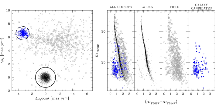
Figure 1: Left: VPD of the relative PMs of the analyzed field. Black dots (within a circle of 1.5 mas yr^-1 from the origin of the VPD) are members of $\omega$ Cen. Field stars are plotted with gray crosses. Objects classified as galaxies in our study are shown as blue circles. The black, dashed circle enclosing these galaxies is centered at $(3.4,6.6)$ mas yr^-1 and has a radius of 1 mas yr^-1. Solid (open) symbols are galaxies employed (discarded) in our estimate of the absolute PM of $\omega$ Cen (see Sect. 3 for detail). Right: Color-magnitude diagrams of all objects in the analyzed field.

A detailed description of the data reduction and relative-PM computation can be found in Paper II. In the following, we provide a brief overview.

We performed our analysis on the _flt exposures corrected by the official pipeline for charge-transfer-efficiency (CTE) defects (see Anderson & Bedin 2010 for the description of this empirical correction). For each camera/filter combination, we extracted positions and fluxes of all detectable sources by point-spread-function (PSF) fitting in a single finding wave without removing the neighbor stars prior to the fit. We used empirical, spatial- and time-varying PSFs obtained by perturbing the publicly available “library” PSFs (see Bellini et al., 2017a). Finally, we corrected the stellar positions for geometric distortion using the solutions of Anderson & King (2006), Bellini & Bedin (2009) and Bellini, Anderson, & Bedin (2011).

We set up a common reference-frame system (“master frame”) for each epoch/camera/filter, which is used to cross-correlate the available single-exposure catalogs. We made use of the Gaia Data Release 1 (DR1, Gaia Collaboration et al., 2016a, b) catalog to (i) set a master-frame pixel scale of 40 mas pixel^-1 (that of WFC3/UVIS detector) and (ii) orient our system with X/Y axes parallel to East/North. Then, we iteratively cross-identified the stars in each catalog with those on the master frame by means of six-parameter linear transformations.

Following Bellini et al. (2017a), we performed a “second-pass” photometry stage by using the software KS2, an evolution of the code used to reduce the ACS Globular Cluster Treasury Survey data in Anderson et al. (2008), and we measured stellar positions and fluxes simultaneously by using individual epochs/filters/exposures at once. We set KS2 to examine F606W- and F814W-filter images to detect every possible object, and then to measure them also in all other filters. Stellar positions and fluxes were measured by re-fitting the PSF in the neighbor-subtracted images. Differently from Bellini et al. (2017a), we are interested not only in the stellar members of $\omega$ Cen, but also field objects (stars and galaxies) that might have moved with respect to $\omega$ Cen by more than 2 pixels (the KS2 method #1 searching radius) between two epochs. Therefore, we executed KS2 independently for the GO-9444+10101 and GO-14118+14662 data to avoid mismatching objects. Finally, our instrumental magnitudes were calibrated onto the Vega magnitude system.

The KS2 software also provides positions and fluxes for detected objects in each raw exposure. Using neighbor-source subtraction, crowded-field issues that might affect the first-pass approach were reduced. Therefore, we employed these raw, KS2-based catalogs to measure the PMs instead of those produced by the first-pass photometry.

PMs were computed using the same methodology described in Bellini et al. (2014). The cornerstones of their iterative procedure are (i) transforming the position of each object as measured in the single catalog/epoch on to the master-frame system, and (ii) fitting a straight line to these transformed positions as a function of the epoch. The slope of this line, computed after several outlier-rejection stages, is a direct measurement of the PM. We refer to Bellini et al. (2014) and Paper II for a detailed description of the PM extraction and systematic corrections.

Because the transformations that relate positions measured in one exposure to those in another were based on cluster stars, by construction, the PM of each star is measured with respect to the average cluster motion. Therefore, the distribution of $\omega$ Cen stars is centered on the origin of the vector-point diagram (VPD), while foreground/background objects are located in different parts of the VPD.

The relative PMs of the objects in our field are shown in Fig. 1. Three groups of objects are clearly distinguishable in the VPD:  
1) cluster stars, centered in the origin of the VPD, with observed dispersion of about 0.34 mas yr^-1 along both $\Delta\mu_{\alpha}\cos\delta$ and $\Delta\mu_{\delta}$ (black points); 
2) background galaxies, clustered in a well-defined location $\sim 7.5$ mas yr^-1 from the mean motion of $\omega$ Cen with a dispersion of 0.40 and 0.32 mas yr^-1 along $\Delta\mu_{\alpha}\cos\delta$ and $\Delta\mu_{\delta}$, respectively (blue circles); 
3) field stars, characterized by a broad distribution at positive $\Delta\mu_{\delta}$ and large negative $\Delta\mu_{\alpha}\cos\delta$, and a narrow tail ending at the galaxy location (gray crosses).

In Paper II we focused on the internal kinematics of the multiple stellar populations hosted in $\omega$ Cen, so that only cluster stars with high-precision PMs were analyzed. In this paper we focus on the global, absolute motion of the cluster. Therefore, we require high accuracy but not necessarily high precision, as was the case in Paper II. As a consequence, we make use of all objects with a PM measurement in our catalog.

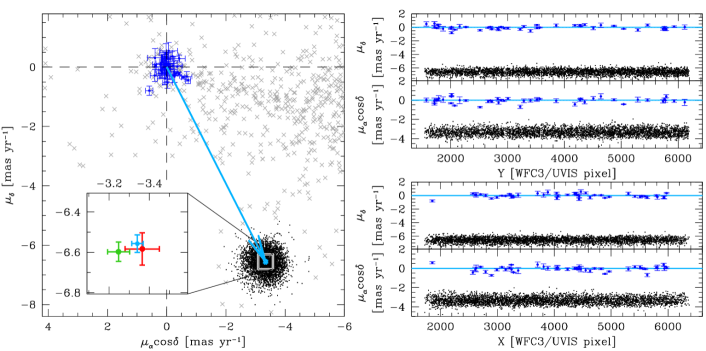
Figure 2: Left: VPD of the absolute PMs in equatorial coordinates of $\omega$ Cen. Black dots and gray crosses represent $\omega$ Cen stars and field objects, respectively. The blue points (with error bars) are the galaxies actually used to compute the absolute PM. The azure arrow indicates the motion of $\omega$ Cen stars with respect to the (fixed) galaxies, the error bars our $\sigma$ uncertainty in the absolute PM value. In the inset, the green and red points (with error bars) are the absolute PMs measured using only F606W- and F814W-filter exposures, respectively (see text for detail). Right: $\mu_{\alpha}cos\delta$ and $\mu_{\delta}$ as a function of X (bottom panels) and Y (top panels) master-frame positions. We omitted field stars for clarity. The dashed, azure stripes represent the absolute PM $\pm\sigma$ error in each component. No systematic trend arises from these plots, proof of the robustness of our PMs.

3 Absolute proper motions

The first step is to link our relative PMs to an absolute reference-frame system. This can be done in two ways: indirectly (by relying on an external catalog of absolute positions), and directly (by computing PMs with respect to fixed sources in the sky, e.g., galaxies).

For the former approach, we can cross-identify cluster members with catalogs providing absolute PMs like the Hipparcos-Tycho (Høg et al., 2000) or the UCAC5 (Zacharias, Finch, & Frouard, 2017), and compute the zero-point offset to be applied to our PMs. Unfortunately, the only stars in common with the UCAC5 catalog are saturated even in the short exposures and are not suitable for astrometry.

Alternatively, we could use the Gaia catalog as a reference. Although intriguing, the major drawback is that only 130 stars are found in common between our catalog and Gaia, and none of them is present in the Tycho-Gaia Astrometric Solution (TGAS), thus preventing us to indirectly register our PMs into an absolute reference frame. Note that TGAS sources would be saturated in our images as is the case of the objects in common with UCAC5 catalog, hence not useful for the registration.

The direct way consists in estimating the absolute PM from our data set using background galaxies in the field as a reference (cf., Bedin et al. 2003, 2006; Milone et al. 2006; Bellini et al. 2010; Massari et al. 2013; Sohn et al. 2015), which is the method we followed.

We started by identifying by eye the center of the distribution of the many galaxy-like objects in the VPD (see Fig. 1). We defined a sample as all objects within a circle of 1 mas yr^-1 from the preliminary center of that group (black, dashed circle in Fig. 1). We then visually inspected the stacked images and rejected all fuzzy galaxies (i.e., objects without a well-defined, point-source-like core), object close to saturated stars or their bleeding columns, and sources which could not be excluded as stars. At the end of our purging process, we are left with 45 galaxies, whose trichromatic rasters are shown in appendix A. Given the tightness of the galaxy distribution in the VPD, it is clear that the positions of these galaxies are measured quite well, even compared to the more plentiful cluster members.

We measured the 5$\sigma$-clipped median value of the PMs in each coordinate for the surviving galaxies. This median value (with the opposite sign) represents the absolute PM of $\omega$ Cen stars at the position of our field F1 (Fig. 2). We find:

$$(\mu_{\alpha}\cos\delta,\mu_{\delta})_{\rm@F1}$$

$$=$$ (1)

$$(-3.341\ \pm\ 0.028,-6.557\ \pm\ 0.043)\textrm{ mas yr${}^{-1}$ .}$$

The quoted errors are the standard error to the mean.

In the right-hand panels of Fig. 2 we also show the absolute PMs along the $\mu_{\alpha}\cos\delta$ and $\mu_{\delta}$ directions as a function of the X and Y positions on the master frame. We find no systematic trends in the PM distribution of either galaxies or $\omega$ Cen stars. Magnitude- and color-dependent systematic errors are also not present in our PMs as shown in Fig. 3 of Paper II.

The cores of our selected galaxies are resolved by , and the galaxies themselves may have different flux distributions and shapes if observed through different filters. As such, the centroid of a galaxy could differ if measured with different filters, resulting in biased PM measurements. Furthermore, Bellini, Anderson, & Bedin (2011) noted that blue and red photons are refracted differently when they pass through the fused-silica window of the CCD of the WFC3/UVIS detector, even if such effect is marginal for filters redder than 3000 Å.

To assess the contributions of these effects to our absolute-PM estimate, we re-computed the relative PMs as described in Paper II in two ways: (1) using only F606W images, and (2) using only F814W images. We then measured the absolute PM of the cluster in both cases, and compared the results with our original estimate. In the inset of the left-hand panel of Fig. 2, we plot the original (in azure), F606W- (in green) and F814W-based (in red) absolute PMs for the cluster. The three absolute PMs are in agreement (well within the error bars), meaning that the galaxy morphology and color effects have negligible impacts in our measurements.

Our observations were obtained in different periods of the year and, as such, our absolute-PM estimate might include an annual-parallax term. However, the contribution of the annual parallax would be of about 0.025 mas yr^-1 at most (by assuming a distance of $\omega$ Cen of 5.2 kpc, Harris, 1996, 2010 edition), a value of the order of our absolute-PM uncertainties.

Furthermore, it is worth noting that our observations were achieved in July (2002), December (2005) and August (2015 and 2017). The highest contribution of the annual parallax would take place if the PM of the galaxies (the parallax effect on $\omega$ Cen stars reflects on background objects because we computed the PMs in a relative fashion) was obtained by employing 2002–2005 or 2005–2015 (or 2017) epoch pairs. However, the PM of 43 out of the 45 galaxies we used in our absolute-PM analysis was computed by adopting all observations at our disposal, for a total temporal baseline of 15.1 yr. Therefore, the fit of the PM is well constrained by the first- and last-epoch observations (at about the same phase in the Earth orbit), and the slope of the straight line (the PM) is expected to be affected by a term much lower than 0.025 mas yr^-1. For all these reasons, we expect the annual parallax to be negligible and we chose not to correct it.

3.1 Cluster rotation

It is well-established that $\omega$ Cen rotates in the plane of the sky (e.g., vL00; Freeman 2001; van Leeuwen & Le Poole 2002; van de Ven et al. 2006, hereafter vdV06). We can also infer the presence of rotation directly from our VPDs. Heyl et al. (2017) showed that the skeweness in the PMs of 47 Tuc is a signature of the differential rotation of the cluster, confirming previous results of the multiple-field PM analysis made by Bellini et al. (2017d). As discussed in Paper II, the PMs of $\omega$ Cen are also skewed in the tangential direction, consistent with cluster rotation.

Therefore, the PM of $\omega$ Cen we obtained in our analysis is a combination of the center of mass (COM) motion and the internal cluster rotation at the position of the field F1. The four fields observed in our large program of $\omega$ Cen are located at different position angles and distances from the cluster center (see Fig. 1 of Paper II), and observations for the other three fields are still ongoing. When all the scheduled multiple-epoch observations are completed for all the fields, we will be able to make a precise measurement of the rotation of the cluster. Here, we use the kinematic analyses of vdV06, in which they adopted the PM catalog of vL00 to derive the rotation of $\omega$ Cen.

Our field is 17 arcmin away from the center of $\omega$ Cen, and projection effects (because of the different line of sight between the COM and our field F1) can produce an additional perspective PM component. In order to measure the PM of the COM of $\omega$ Cen, we must also remove the contribution of the projection from our estimate.

The size of our field is small as compared to its distance from the center of $\omega$ Cen. Therefore, we assumed that, at the first order, the effects of perspective and internal rotation are the same for all stars in field F1. Because of this, we corrected the absolute-PM measurement we inferred in Sect. 3 and not the PM of each individual star.

First, we computed the contribution of perspective using the prescription given in van der Marel et al. (2002). By adopting as the reference position of our field the average position of all its stars, we find:

$$(\mu_{\alpha}\cos\delta,\mu_{\delta})_{\rm Perspective}$$

$$=$$ (2)

$$(0.008,0.043)\textrm{ mas yr${}^{-1}$ .}$$

We then assessed the contribution of the cluster rotation. Table 3 of vdV06 reports the mean PM of $\omega$ Cen in different polar sectors in the plane of the sky. These velocities size the amount of the rotation in different locations of the cluster. After we identified in which polar sector our field lies, we transformed the corresponding PM values in Table 3 of vdV06 from the axisymmetric reference frame adopted in their study to the equatorial reference frame, and decomposed these PMs in the corresponding radial and tangential components. Since we are only interested in the amount of rotation, we just need to correct our PMs by the tangential component. Finally, we transformed these PM values back to the equatorial coordinate system. The expected contribution of cluster rotation to the absolute PM is:

$$(\mu_{\alpha}\cos\delta,\mu_{\delta})_{\rm Rot}$$

$$=$$ (3)

$$(-0.111,0.116)\textrm{ mas yr${}^{-1}$ .}$$

By subtracting the perspective and the rotation components to our absolute PM at the position of our field F1, we obtain our best estimate of the absolute PM of the COM of $\omega$ Cen:

$$(\mu_{\alpha}\cos\delta,\mu_{\delta})_{\rm COM}$$

$$=$$ (4)

$$(-3.238\pm 0.028,-6.716\pm 0.043)\textrm{ mas yr${}^{-1}$ .}$$

The difference between the absolute PM at the position of our field F1 and that of the COM is of about 0.19 mas yr^-1, dominated by cluster rotation. This correction is qualitatively in agreement with that expected by Fig. 6 of vdV06, both in magnitude and direction.

It is important to note that vdV06 employed the PM catalog of vL00, which is known to have severe color- and magnitude-dependent systematic effects as described by Platais et al. (2003). The uncertainty in the COM PM listed above includes only random errors, and no systematic uncertainties in the rotation correction. If the $\sim 4$ km s^-1 PM rotation measured by vdV06 is inaccurate by more than $\sim 30$%, then this systematic error dominates the error budget.

To determine the corresponding Galactocentric velocity of the COM, we adopt a Cartesian Galactocentric coordinate system ($X,Y,Z$), with the origin at the Galactic Center, the $X$-axis pointing in the direction from the Sun to the Galactic Center, the $Y$-axis pointing in the direction of the Sun’s Galactic rotation, and the $Z$-axis pointing towards the Galactic North Pole. We use the same quantities and corresponding uncertainties for the Sun and for $\omega$ Cen as in Sect. 5 below (see Tables 3 and 3). This implies a Galactocentric $(X,Y,Z)$ position

$${\vec{r}}=(-5.1,-3.9,1.3)\textrm{ kpc ,}$$ (5)

and a Galactocentric velocity vector

$${\vec{v}}=(97.9\pm 3.0,-18.0\pm 8.6,-80.2\pm 7.2)\textrm{ km s${}^{-1}$ .}$$ (6)

The corresponding Galactocentric radial and tangential velocities are

$$(V_{\rm rad},V_{\rm tan})=(-82.0\pm 7.8,98.1\pm 10.4)\textrm{ km s${}^{-1}$ ,}$$ (7)

and the observed total velocity with respect to the Milky Way is

$$v\equiv|{\vec{v}}|=(127.9\pm 3.5)\textrm{ km s${}^{-1}$ .}$$ (8)

The listed uncertainties were obtained from a Monte-Carlo scheme that propagates all observational distance and velocity uncertainties and their correlations, including those for the Sun.

3.2 Field stars: who is who

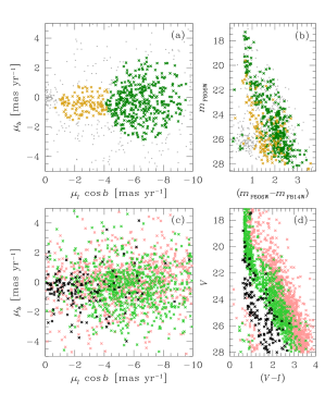
Figure 3: Comparison between observed (top panels) and simulated (bottom panels) VPDs in Galactic coordinates (left-hand panels) and color-magnitude diagrams (right-hand panels). In panels (a) and (b) we show galaxies/field stars with gray dots and highlight the two investigated groups in gold and dark green. In panels (c) and (d) we color-code the simulated halo, thick and thin disk stars in black, light green and pink, respectively.

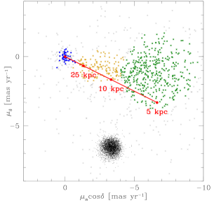
Figure 4: VPD of the absolute PMs in equatorial coordinates highlighting the galaxies (in blue) and the two groups of field stars analyzed in Sect. 3.2 (in gold and dark-green colors). $\omega$ Cen stars and the remaining field objects are shown with black dots and gray crosses, respectively. The red line marks the expected reflex motion of stars at different Galactocentric distances (see text for detail).

The VPDs in Figs. 1 and 2 reveal the presence of two main field-star components. In panel (a) of Fig. 3 we highlighted them with gold and dark-green crosses. These two groups of stars also show different loci in the color-magnitude diagrams (panel b). To identify the stellar populations they belong to, we compared the observed absolute PMs of field stars in our catalog to those of the Besançon models (Robin et al., 2003). We simulated stars out to 50 kpc in a $6\times 6$ arcmin² region centered on our field. We assumed the photometric and PM errors to be zero since we are only interested in tagging each component of the field. The final simulated sample is composed of halo (shown with black crosses in the bottom panels of Fig. 3), thin- (pink crosses), and thick-disk (light-green crosses) stars.

Both color-magnitude diagrams and VPDs (in Galactic coordinates) in Fig. 3 suggest that the broad group of field stars in our observed VPD is mainly constituted by disk stars, while the narrow stream connecting the distributions of disk stars to the galaxies is associated with halo stars.

En passant, we find broad agreement between observed and simulated PMs, an independent validation of the theoretical predictions of Besançon models.

We can reach similar conclusions by considering that, when we look at the stars along the line of sight toward $\omega$ Cen, we see reflex motion due to the motion of the Sun. By assuming a Sun motion in Galactocentric reference frame given in Sect. 5 below (see Table 3), we expect a reflex proper motion of:

$$\left\{\begin{array}[]{rl}\mu_{\alpha}\cos\delta&=-6.391\times(5.2/d)\textrm{ mas yr${}^{-1}$}\\ \mu_{\delta}&=-3.190\times(5.2/d)\textrm{ mas yr${}^{-1}$ ,}\end{array}\right.$$ (9)

with $d$ the distance of a given star from the Galactic center in kpc. For hypothetical stars that stand still in the Galactocentric reference frame, this motion is equal to the observed PM. In the VPD in Fig. 4, we used the equations above to mark the expected location of a given object at different Galactocentric distances.

Galaxies and very-distant halo stars have no motions in the Galactocentric reference frame. Therefore, they fall at the large distance end of the red line with a small scatter (because the PMs induced by their peculiar velocities at large distances are small). Intermediate-distance stars are in the inner disk and bulge, and these stars have a orbital motion in the Milky Way. As such, they do not fall exactly along the line. Finally, nearby stars have a large scatter about the line because of their large PMs induced by peculiar velocities, even if the latter are relatively small.

Looking at Fig. 4, it seems that gold points are much closer to the straight line and at large distances, as expected by halo and intermediate-disk stars. Green objects have instead a broad distribution far from the red line, suggesting that they are nearby disk stars.

Table 1: List of the absolute PM of $\omega$ Cen in the literature and computed in this paper.

ID	Reference	$\bf\mu_{\alpha}\cos\delta$	$\bf\mu_{\delta}$	Extragalactic?	Notes
		[mas yr-1]	[mas yr-1]
M65	Murray, Candy, & Jones (1965)	$+0.5\pm 0.6$	$-7.7\pm 0.5$	No
W66	Woolley (1966)	$-3.6\pm 0.5$	$-6.0\pm 0.5$	No	(a)
D99	Dinescu et al. (1999)	$-4.88\pm 0.35$	$-3.47\pm 0.34$	Yes	(b)
		$-5.08\pm 0.35$	$-3.57\pm 0.34$	Yes
vL00	van Leeuwen et al. (2000)	$-3.97\pm 0.41$	$-4.38\pm 0.41$	No	(c)
G02	Geffert et al. (2002)	$-4.2\pm 0.5$	$-5.1\pm 0.5$	No
		$-4.1\pm 0.5$	$-4.8\pm 0.5$	No	(d)
K13	Kharchenko et al. (2013)	$-6.01\pm 0.25$	$-5.02\pm 0.25$	No	(e)
vL00 (@F1)	This paper	$-4.17\pm 0.41$	$-4.31\pm 0.41$	No	(f)
vL00 (COM)	This paper	$-4.06\pm 0.41$	$-4.43\pm 0.41$	No	(g)
HSOY (@F1)	This paper	$-4.08\pm 0.44$	$-6.68\pm 0.26$	No
HSOY (All)	This paper	$-3.21\pm 0.15$	$-6.51\pm 0.14$	No	(h)
UCAC5 (@F1)	This paper	$-4.10\pm 0.27$	$-7.00\pm 0.26$	No
UCAC5 (All)	This paper	$-3.30\pm 0.03$	$-6.80\pm 0.03$	No	(h)
L18 (@F1)	This paper	$-3.341\pm 0.028$	$-6.557\pm 0.043$	Yes
L18 (COM)	This paper	$-3.238\pm 0.028$	$-6.716\pm 0.043$	Yes	(i)

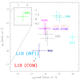
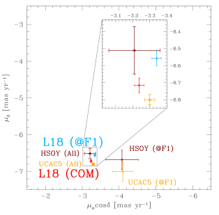
Figure 5: Left: comparison between the absolute PM of $\omega$ Cen obtained with data and the literature. The azure and red points represent the absolute PM at the distance of our field (L18 @F1) and of the COM (L18 COM, obtained with the corrections described in Sect. 3.1), respectively. Using the IDs listed in Table 1, we plot the values of W66 in dark blue, D99 in turquoise, vL00 in magenta, G02 in gray and K13 in cyan. The value of M65 is shown as a light-green point in the inset. The value of $\omega$ Cen COM absolute PM obtained from the corrected vL00 PMs (see text for detail) is shown in purple. The value obtained using stars in vL00 catalog (with PMs corrected only for perspective and solid-body rotations) at the same position of our F1 field (in pink) is plot as reference. Right: absolute-PM of $\omega$ Cen at the position of our field F1 on the same scale obtained by using UCAC5 (in orange) and HSOY (in brown) catalogs. The error bars are the standard errors to the mean. The orange and brown triangles represent the absolute PM of $\omega$ Cen computed using the PMs of all likely cluster members (not only those in the field F1) in UCAC5 and HSOY catalogs, respectively. In the inset, we zoom-in around the location of our absolute-PM estimates.

4 Comparison with the literature

The current estimates of the absolute PMs of $\omega$ Cen available in the literature are collected in Table 1 and are shown in the left-hand panel of Fig. 5. With the interesting exception of the value of Geffert et al. (2002) obtained by linking the PM catalog of Murray, Candy, & Jones (1965) and Woolley (1966) to the Tycho 2 catalog (dark-blue point with label W66), the disagreement between our result and the literature values is clear. For example, there is a difference of more than 2 mas yr ^-1 in modulus and about 30^∘ and 15^∘ in orientation, resulting in 9$\sigma$ and 5$\sigma$ discrepancies, between our value and those of D99 and vL00, respectively.

To understand whether our methodology or the analyzed field can be at the basis of these discrepancies, as test we downloaded the publicly-available vL00 catalog and computed the absolute PM of $\omega$ Cen using PMs therein. We limited our analysis to 45 cluster members (membership probability greater than 85% in the vL00 catalog) at the position of our field F1.

vdV06 pointed out that the PMs of vL00 are affected by perspective and solid-body (due to a misalignment between the photographic plates of different epochs) rotations. Therefore, we corrected the perspective component as described in Sect. 3.1; and the solid-body part as described in vdV06 (Eq. 7), using the average position of the 45 stars as reference, and transforming the corresponding PM correction from the $\omega$ Cen axisymmetric reference frame to the equatorial reference frame. By applying these two corrections, we computed the absolute PM at the position of our field F1 (pink point in the left-hand panel of Fig. 5). Finally, we removed the effect of the cluster rotation as described in Sect. 3.1 and obtained the absolute PM of $\omega$ Cen COM. The result is shown in the left-hand panel of Fig. 5 as a purple point. Again, the difference with our absolute PM estimates is about 5$\sigma$.

We also measured the absolute PM of $\omega$ Cen using the absolute PMs published in the UCAC5 and “Hot Stuff for One Year” (HSOY, Altmann et al., 2017) catalogs. We chose these two catalogs because both of them employ the Gaia DR1 catalog to link their astrometry to an absolute reference-frame system. The absolute-PM measurements were obtained by using 45 cluster members, selected on the basis of their location in the CMD and in the VPD, at the same location of the stars analyzed in our paper. In the right-hand panel of Fig. 5 we show the absolute PM of $\omega$ Cen at the distance of our field F1 (i.e., without considering the effect of the perspective and cluster rotation) for UCAC5 (orange point) and HSOY (brown point) catalogs. Both UCAC5 and HSOY values are closer to our measurements than to those in the literature. For completeness, we also computed the PM of $\omega$ Cen using all likely cluster members in the UCAC5 and HSOY catalogs, not only those at the position of our field F1. By considering a more populated sample in the computation (2394 for UCAC5 and 339 for HSOY), the agreement with our estimate becomes tighter (orange and brown triangles for UCAC5 and HSOY, respectively, in the right-hand panel of Fig. 5). Note that the errors for UCAC5 value are smaller than those for our estimate because of the larger number of considered objects. This external check further strengthens our result.

Table 2: Parameters employed for the Galactic Potential.

Parameter	Value	References
$R_{0}$	$8.30\pm 0.23$ kpc	(a)
${\Theta}_{0}$	$239\pm 7$ km s-1	(a)
$(U,V,W)_{\odot}$	$(-11.10\pm 1.20,12.24\pm 2.10,7.25\pm 0.60)$ km s-1	(a,b)
Galactic Bar
Mass	$1.1\times 10^{10}$ M⊙	(c,d)
Present position of major axis	20∘	(e)
$\Omega_{\rm bar}$	40, 45, 50 km s-1 kpc-1	(f,g)
Cut-off radius	3.28 kpc	(d,h,i)
Spiral Arms
$M_{\rm arms}/M_{\rm disk}$	0.05	(l)
Scale length	5.0 kpc	(m)
Pitch angle	15.5∘	(n)
Angular velocity	25 km s-1 kpc-1	(m,o)

Table 3: $\omega$ Cen parameters adopted in the orbit computation.

Parameter	Value	Reference
$(\alpha,\delta)_{\rm J2000}$	($13^{\rm h}26^{\rm m}47^{\rm s}\!\!.24$,$-47^{\circ}28^{\prime}46^{\prime\prime}\!\!.45$)	(a)
Radial Velocity	$232.2\pm 0.7$ km s-1	(b,c)
Distance	$5.20\pm 0.25$ kpc	(d)
$X$	$-5.1$ kpc
$Y$	$-3.9$ kpc
$Z$	1.3 kpc
Dinescu et al. (1999)
$\mu_{\alpha}\cos\delta$	$(-5.08\pm 0.35)$ mas yr-1
$\mu_{\delta}$	$(-3.57\pm 0.34)$ mas yr-1
$v_{X}$	58.0 km s-1
$v_{Y}$	$-22.8$ km s-1
$v_{Z}$	0.2 km s-1
Our paper (L18 @F1) (∗)
$\mu_{\alpha}\cos\delta$	$(-3.341\pm 0.028)$ mas yr-1
$\mu_{\delta}$	$(-6.557\pm 0.043)$ mas yr-1
$v_{X}$	95.7 km s-1
$v_{Y}$	$-18.4$ km s-1
$v_{Z}$	$-76.1$ km s-1

5 The orbit of $\omega$ Cen

In order to analyze the repercussions of the new PM determinations on the orbit of $\omega$ Cen, we computed the orbit in two detailed mass models based on the Milky Way Galaxy.

The first model is based on an escalation of the axisymmetric Galactic model of Allen & Santillan (1991), for which we converted its bulge component into a prolate bar with the mass distribution given in Pichardo, Martos, & Moreno (2004). We also included the 3D spiral-arm model considered in Pichardo et al. (2003) to explore any possible effect of the spiral arms on $\omega$ Cen. For this first potential, we computed the minimum and maximum distances from the Galactic center, the maximum vertical distance from the Galactic plane, the orbital eccentricity, and the angular momentum. The eccentricity $e$ is defined as:

$$e=(R_{\rm max}-R_{\rm min})/(R_{\rm max}+R_{\rm min})\textrm{ ,}$$ (10)

where $R_{\rm min}$ and $R_{\rm max}$ are successive minimum and maximum distances from the Galactic rotation axis (i.e., $R$ is the distance in cylindrical coordinates), respectively.

From a gravitational perspective, the most influential part of the Galaxy for dynamically hot (eccentric) stellar clusters or dwarf galaxies is the inner region, where the bar and the maximum mass concentration of the Galaxy are located. An accurate model of the central part of the Galaxy is paramount for an accurate determination of the orbit. For these reasons, we performed a second experiment using the new galaxy-modeling algorithm called GravPot16 (Fernández-Trincado et al., 2017a, 2018) that specifically attempts to model the inner Galactic region. GravPot16 is a semi-analytic, steady-state, 3D gravitational potential of the Milky Way observationally and dynamically constrained. GravPot16 is a non-axisymmetric potential including only the bar in its non-axisymmetric components. The potential model is primarily the superposition of several composite stellar components where the density profiles in cylindrical coordinates, $\rho_{i}(R,z)$, are the same as those proposed in Robin et al. (2003, 2012, 2014), i.e., a boxy/peanut bulge, a Hernquist stellar halo, seven stellar Einasto thin disks with spherical symmetry in the inner regions, two stellar sech² thick disks, a gaseous exponential disk, and a spherical structure associated with the dark matter halo. A new formulation for the global potential of this Milky Way density model will be described in detail in a forthcoming paper (Fernández-Trincado et al., 2018). For the second potential, we computed the orbits in a Galactic non-inertial reference frame in which the bar is at rest, and we specifically examined the orbital Jacobi constant per unit mass, $E_{\rm J}$, which is conserved in this reference frame. The orbital energy $E_{\rm J}$ per unit of mass is defined as:

$$E_{\rm J}=\frac{1}{2}\vec{v}^{2}+\Phi_{\rm axi}+\Phi_{\rm non-axi}-\frac{1}{2}|\vec{\Omega}_{\rm bar}\times\vec{R}|^{2}\textrm{ ,}$$ (11)

with $\Phi_{\rm axi}$ and $\Phi_{\rm non-axi}$ the gravitational potential of the axisymmentric and non-axisymmentric (in this case the bar) Galactic potential, respectively; $\Omega_{\rm bar}$ the angular velocity gradient, and $R$ the vector $\vec{r}$ of the particles/stars.

For the potential of the bar, we assumed (i) a total mass of $1.1\times 10^{10}$ M_⊙, (ii) an angle of 20^∘ for the present-day orientation of the major axis of the bar, (iii) an angular velocity gradient of the bar $\Omega_{\rm bar}$ of 40, 45, and 50 km s^-1 kpc^-1, and (iv) a cut-off radius for the bar of $R_{\rm cut}=3.28$ kpc. The bar potential model was computed using a new mathematical technique that considers ellipsoidal shells with similar linear density (Fernández-Trincado et al., 2018). Table 3 summarizes the parameters employed for the Galactic potential, the position and velocity of the Sun in the Local Standard of Rest, and the properties of the bar and of the spiral arms.

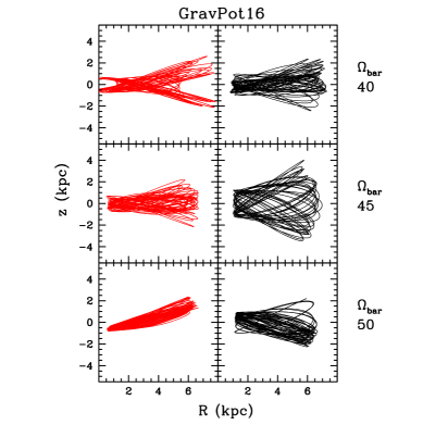
Figure 6: Meridional orbits of $\omega$ Cen for the last 2 Gyr for our first Galactic potential, with an angular velocity gradient of the Galactic bar of 40 (top row), 45 (middle row), 50 (bottom row) km s^-1 kpc^-1. The orbits in the first column (red lines) employed the PM value of D99, while the orbits in the second and third columns (black lines) adopted those computed in this paper. In the third column, the orbits were computed by adding the spiral arms with an angular velocity of 25 km s^-1 kpc^-1.

Figure 7: Same as Fig. 7 but with orbits calculated assuming the second Galactic potential..

Hereafter, we discuss the results achieved by employing the absolute-PM value measured for the stars in field F1. We also ran the corresponding calculations for the estimated COM PM and found a negligible difference (e.g., comparable perigalacticons, apogalacticons, region covered by the orbit) as expected given the small PM difference between the two estimates. The COM is physically the correct quantity to use, but by using the value for F1 we remove any dependence on the assumed, and possibly uncertain, correction for the PM rotation of the cluster (and note that the perspective and rotation corrections for $\omega$ Cen are smaller than the uncertainty in the azimuthal velocity of the Sun). The other $\omega$ Cen parameters are listed in Table 3. Finally, we also calculated, for comparison, the $\omega$ Cen orbit by assuming the PM value of D99.

Figures 7 and 7 present the orbits of $\omega$ Cen obtained by considering the first and the second Galactic potential, respectively. For each value of the angular velocity gradient of the Galactic bar (different rows) we investigated, we show the meridional orbit of $\omega$ Cen obtained using the absolute-PM value of D99 (red lines in the left columns) and that computed with data in our paper (black lines in the other columns). Furthermore, in the rightmost column of Fig. 7, we display the orbit calculated by including the spiral arms in the computation.

Looking at Fig. 7, some differences can be discerned between the different orbits. The radial excursions of the orbit of $\omega$ Cen seem to increase slightly with the new PM value, while the vertical excursions remain similar regardless of the PM adopted. The main difference between the new and the literature PM values is the larger (about half a kpc) perigalactic distance obtained with the PM computed in our paper. This more distant approach to the innermost part of the Galaxy likely means a larger survival expectancy for the cluster.

Examining the impact of the spiral arms, contrary to intuition we find that the spiral arms can influence the orbit, although slightly. However, the differences with this and the bar-only potential model is statistical and does not change the fundamental properties of the orbit (i.e., perigalacticons and apogalacticons).

Finally, by comparing Figs. 7 and 7, we found that both models seem to reproduce a similar behavior in the radial and vertical excursions, and no important differences due to the details of the modeling are detectable. This means that probably the most important features on models that influence the orbital behavior of this particular cluster are the density law and the angular velocity of the bar that are basically the same in both models.

In Tables 5 and 5 we present average orbital parameters for $\omega$ Cen for the various Galactic potentials obtained by using a simple Monte Carlo procedure to vary the initial conditions. 500 orbits for the first potential and 50 000 orbits for the second potential are computed under 1$\sigma$ variation of the absolute PMs, distance, radial velocity, and Solar motion. The errors provided for these parameters were assumed to follow a Gaussian distribution. The parameters listed in the Tables are the minimum and maximum distances to the Galactic center, the maximum distance from the Galactic plane, and the orbital eccentricity. In Table 5 we also provide the angular momentum, while in Table 5 we give the orbital Jacobi energy.

6 Conclusions

As part of the large program GO-14118+14662 on $\omega$ Cen, in this third paper of the series we presented a revised estimate of the absolute PM of this cluster. Thanks to the exquisite -based astrometry and high-precision PMs computed in Paper II, we are able to use background galaxies to link our relative astrometry to an absolute frame. Our measured absolute PM differs significantly from the values available in the literature in magnitude, direction and precision. A comparison with recent catalogs yields instead an excellent agreement.

We also calculated the orbit of $\omega$ Cen with two different models of the potential for the Milky Way Galaxy. The primary difference between the orbits with our new PM and those based on prior estimates is a larger (by about half a kpc) perigalactic distance obtained with our new value. This may imply a larger survival expectancy for the cluster in the inner Galactic environment.

We emphasize that the absolute PM presented here is both an independent (with the exception of the registration of the master-frame absolute scale and orientation with the Gaia DR1 catalog) and direct measurement based on the use of a reference sample of background galaxies. As such, these results presented here provide an external check for future astrometric all-sky catalogs, in particular the upcoming Gaia DR2.

Appendix A Galaxy finding charts

In Fig. 8 we show the trichromatic stacked images of the 45 galaxies used to compute the absolute PM of $\omega$ Cen. Each source is centered in a $51\times 51$ WFC3/UVIS pixel² ($\sim 2\times 2$ arcsec²) stamp. We used F814W, F606W and F336W filters for red, green and blue channels, respectively.

Figure 8: Trichromatic stacked images of the galaxies adopted in our analysis.

References

- Allen & Santillan (1991) Allen C., Santillan A., 1991, RMxAA, 22, 255
- Altmann et al. (2017) Altmann M., Roeser S., Demleitner M., Bastian U., Schilbach E., 2017, A&A, 600, L4
- Anderson (1997) Anderson J., 1997, Ph.D. thesis, Univ. of California, Berkley
- Anderson & King (2006) Anderson J., King I. R., 2006, acs..rept,
- Anderson et al. (2008) Anderson J., et al., 2008, AJ, 135, 2055
- Anderson & Bedin (2010) Anderson J., Bedin L. R., 2010, PASP, 122, 1035
- Anderson & van der Marel (2010) Anderson J., van der Marel R. P., 2010, ApJ, 710, 1032
- Bedin et al. (2003) Bedin L. R., Piotto G., King I. R., Anderson J., 2003, AJ, 126, 247
- Bedin et al. (2004) Bedin L. R., Piotto G., Anderson J., Cassisi S., King I. R., Momany Y., Carraro G., 2004, ApJ, 605, L125
- Bedin et al. (2006) Bedin L. R., Piotto G., Carraro G., King I. R., Anderson J., 2006, A&A, 460, L27
- Bekki & Freeman (2003) Bekki K., Freeman K. C., 2003, MNRAS, 346, L11
- Bellini & Bedin (2009) Bellini A., Bedin L. R., 2009, PASP, 121, 1419
- Bellini et al. (2010) Bellini A., Bedin L. R., Pichardo B., Moreno E., Allen C., Piotto G., Anderson J., 2010, A&A, 513, A51
- Bellini, Anderson, & Bedin (2011) Bellini A., Anderson J., Bedin L. R., 2011, PASP, 123, 622
- Bellini et al. (2013) Bellini A., Anderson J., Salaris M., Cassisi S., Bedin L. R., Piotto G., Bergeron P., 2013, ApJ, 769, L32
- Bellini et al. (2014) Bellini A., et al., 2014, ApJ, 797, 115
- Bellini et al. (2017a) Bellini A., Anderson J., Bedin L. R., King I. R., van der Marel R. P., Piotto G., Cool A., 2017a, ApJ, 842, 6
- Bellini et al. (2017b) Bellini A., Anderson J., van der Marel R. P., King I. R., Piotto G., Bedin L. R., 2017b, ApJ, 842, 7
- Bellini et al. (2017c) Bellini A., Milone A. P., Anderson J., Marino A. F., Piotto G., van der Marel R. P., Bedin L. R., King I. R., 2017c, ApJ, 844, 164
- Bellini et al. (2017d) Bellini A., Bianchini P., Varri A. L., Anderson J., Piotto G., van der Marel R. P., Vesperini E., Watkins L. L., 2017d, ApJ, 844, 167
- Bellini et al. (2018) Bellini A., et al., 2018, arXiv, arXiv:1801.01504
- Bissantz et al. (2003) Bissantz, N., Englmaier, P., & Gerhard, O. 2003, MNRAS, 340, 949
- Brunthaler et al. (2011) Brunthaler A., et al., 2011, AN, 332, 461
- Dinescu et al. (1999) Dinescu D. I., van Altena W. F., Girard T. M., López C. E., 1999, AJ, 117, 277
- Drimmel (2000) Drimmel R., 2000, A&A, 358, L13
- Fernández-Trincado et al. (2015) Fernández-Trincado J. G., Vivas A. K., Mateu C. E., Zinn R., Robin A. C., Valenzuela O., Moreno E., Pichardo B., 2015, A&A, 574, A15
- Fernández-Trincado et al. (2017a) Fernández-Trincado J. G., Robin A. C., Moreno E., Pérez-Villegas A., Pichardo B., 2017a, arXiv, arXiv:1708.05742
- Fernández-Trincado et al. (2017b) Fernández-Trincado J. G., Geisler D., Moreno E., Zamora O., Robin A. C., Villanova S., 2017b, arXiv, arXiv:1710.07433
- Fernández-Trincado et al. (2018) Fernández-Trincado et al. (2018, in preparation)
- Freeman (2001) Freeman K. C., 2001, ASPC, 228, 43
- Gaia Collaboration et al. (2016a) Gaia Collaboration, et al., 2016a, A&A, 595, A1
- Gaia Collaboration et al. (2016b) Gaia Collaboration, et al., 2016b, A&A, 595, A2
- Geffert et al. (2002) Geffert M., Hilker M., Geyer E. H., Krämer G.-H., 2002, ASPC, 265, 399
- Gerhard (2002) Gerhard O., 2002, ASPC, 273, 73
- Gerhard (2011) Gerhard O., 2011, MSAIS, 18, 185
- Harris (1996) Harris W. E., 1996, AJ, 112, 1487
- Heyl et al. (2017) Heyl J., Caiazzo I., Richer H., Anderson J., Kalirai J., Parada J., 2017, ApJ, 850, 186
- Høg et al. (2000) Høg E., et al., 2000, A&A, 355, L27
- Kharchenko et al. (2013) Kharchenko N. V., Piskunov A. E., Schilbach E., Röser S., Scholz R.-D., 2013, A&A, 558, A53
- Martinez-Medina et al. (2017) Martinez-Medina, L. A., Pichardo, B., Peimbert, A., & Carigi, L. 2017, MNRAS, 468, 3615
- Mayor et al. (1997) Mayor M., et al., 1997, AJ, 114, 1087
- Massari et al. (2013) Massari D., Bellini A., Ferraro F. R., van der Marel R. P., Anderson J., Dalessandro E., Lanzoni B., 2013, ApJ, 779, 81
- Milone et al. (2006) Milone A. P., Villanova S., Bedin L. R., Piotto G., Carraro G., Anderson J., King I. R., Zaggia S., 2006, A&A, 456, 517
- Milone et al. (2017a) Milone A. P., et al., 2017a, MNRAS, 464, 3636
- Milone et al. (2017b) Milone A. P., et al., 2017b, MNRAS, 469, 800
- Murray, Candy, & Jones (1965) Murray C. A., Candy M. P., Jones D. H. P., 1965, RGOB, 100, 81
- Navarrete et al. (2017) Navarrete C., Catelan M., Contreras Ramos R., Alonso-García J., Gran F., Dékány I., Minniti D., 2017, A&A, 606, C1
- Pichardo et al. (2003) Pichardo B., Martos M., Moreno E., Espresate J., 2003, ApJ, 582, 230
- Pichardo, Martos, & Moreno (2004) Pichardo B., Martos M., Moreno E., 2004, ApJ, 609, 144
- Pichardo et al. (2012) Pichardo B., Moreno E., Allen C., Bedin L. R., Bellini A., Pasquini L., 2012, AJ, 143, 73
- Platais et al. (2003) Platais I., Wyse R. F. G., Hebb L., Lee Y.-W., Rey S.-C., 2003, ApJ, 591, L127
- Portail et al. (2015) Portail M., Wegg C., Gerhard O., Martinez-Valpuesta I., 2015, MNRAS, 448, 713
- Reijns et al. (2006) Reijns R. A., Seitzer P., Arnold R., Freeman K. C., Ingerson T., van den Bosch R. C. E., van de Ven G., de Zeeuw P. T., 2006, A&A, 445, 503
- Roeser, Demleitner, & Schilbach (2010) Roeser S., Demleitner M., Schilbach E., 2010, AJ, 139, 2440
- Robin et al. (2003) Robin A. C., Reylé C., Derrière S., Picaud S., 2003, A&A, 409, 523
- Robin et al. (2012) Robin A. C., Marshall D. J., Schultheis M., Reylé C., 2012, A&A, 538, A106
- Robin et al. (2014) Robin A. C., Reylé C., Fliri J., Czekaj M., Robert C. P., Martins A. M. M., 2014, A&A, 569, A13
- Schönrich, Binney, & Dehnen (2010) Schönrich R., Binney J., Dehnen W., 2010, MNRAS, 403, 1829
- Sofue (2015) Sofue Y., 2015, PASJ, 67, 75
- Sohn et al. (2015) Sohn S. T., van der Marel R. P., Carlin J. L., Majewski S. R., Kallivayalil N., Law D. R., Anderson J., Siegel M. H., 2015, ApJ, 803, 56
- Sormani, Binney, & Magorrian (2015) Sormani M. C., Binney J., Magorrian J., 2015, MNRAS, 454, 1818
- van de Ven et al. (2006) van de Ven G., van den Bosch R. C. E., Verolme E. K., de Zeeuw P. T., 2006, A&A, 445, 513
- van der Marel et al. (2002) van der Marel R. P., Alves D. R., Hardy E., Suntzeff N. B., 2002, AJ, 124, 2639
- van Leeuwen et al. (2000) van Leeuwen F., Le Poole R. S., Reijns R. A., Freeman K. C., de Zeeuw P. T., 2000, A&A, 360, 472
- van Leeuwen & Le Poole (2002) van Leeuwen F., Le Poole R. S., 2002, ASPC, 265, 41
- Woolley (1966) Woolley R. V. D. R., 1966, ROAn, 2,
- Zacharias et al. (2000) Zacharias N., et al., 2000, AJ, 120, 2131
- Zacharias, Finch, & Frouard (2017) Zacharias N., Finch C., Frouard J., 2017, AJ, 153, 166