The HST large programme on $\omega$ Centauri – II. Internal kinematics

Abstract

In this second installment of the series, we look at the internal kinematics of the multiple stellar populations of the globular cluster $\omega$ Centauri in one of the parallel Hubble Space Telescope (HST) fields, located at about 3.5 half-light radii from the center of the cluster. Thanks to the over 15-year-long baseline and the exquisite astrometric precision of the HST cameras, well-measured stars in our proper-motion catalog have errors as low as $\sim 10\,\mu$as yr^-1, and the catalog itself extends to near the hydrogen-burning limit of the cluster. We show that second-generation (2G) stars are significantly more radially anisotropic than first-generation (1G) stars. The latter are instead consistent with an isotropic velocity distribution. In addition, 1G have excess systemic rotation in the plane of the sky with respect to 2G stars. We show that the six populations below the main-sequence (MS) knee identified in our first paper are associated to the five main population groups recently isolated on the upper MS in the core of cluster. Furthermore, we find both 1G and 2G stars in the field to be far from being in energy equipartition, with $\eta_{\rm 1G}=-0.007\pm 0.026$ for the former, and $\eta_{\rm 2G}=0.074\pm 0.029$ for the latter, where $\eta$ is defined so that the velocity dispersion $\sigma_{\mu}$ scales with stellar mass as $\sigma_{\mu}\propto m^{-\eta}$. The kinematical differences reported here can help constrain the formation mechanisms for the multiple stellar populations in $\omega$ Centauri and other globular clusters. We make our astro-photometric catalog publicly available.

1 Introduction

Table 1: List of HST observations of field F1.

Filter	Exposures	Program ID	PI	Epoch
ACS/WFC (Epoch 1)
F606W	$2\times 1300\,{\rm s}+2\times 1375\,{\rm s}$	9444	King, I. R.	2002/07/03
F814W	$2\times 1340\,{\rm s}+2\times 1375\,{\rm s}$	9444	King, I. R.	2002/07/03
ACS/WFC (Epoch 2)
F606W	$2\times 1285\,{\rm s}+2\times 1331\,{\rm s}$	10101	King, I. R.	2005/12/24
F814W	$4\times 1331\,{\rm s}$	10101	King, I. R.	2005/12/24
WFC3/UVIS (Epoch 3)
F275W	$4\times 1328\,{\rm s}$	14118	Bedin, L. R.	2015/08/23–26
F336W	$4\times 1230\,{\rm s}$	14118	Bedin, L. R.	2015/08/23–26
F438W	$4\times 98\,{\rm s}$	14118	Bedin, L. R.	2015/08/22–26
F606W	$2\times 99\,{\rm s}+2\times 1255\,{\rm s}+2\times 1347\,{\rm s}$	14118	Bedin, L. R.	2015/08/22–23
F814W	$2\times 98\,{\rm s}+2\times 1253\,{\rm s}+2\times 1345\,{\rm s}$	14118	Bedin, L. R.	2015/08/20–21
WFC3/IR (Epoch 3)
F110W	$7\times 142\,{\rm s}+14\times 1302\,{\rm s}$	14118	Bedin, L. R.	2015/08/19–24
F160W	$7\times 142\,{\rm s}+14\times 1302\,{\rm s}$	14118	Bedin, L. R.	2015/08/24–26
WFC3/UVIS (Epoch 4)
F275W	$4\times 1229\,{\rm s}$	14662	Bedin, L. R.	2017/08/19–20
F336W	$4\times 1143\,{\rm s}$	14662	Bedin, L. R.	2017/08/19–20
F438W	$3\times 95\,{\rm s}+1\times 104\,{\rm s}$	14662	Bedin, L. R.	2017/08/19–20
F606W	$2\times 104\,{\rm s}+2\times 1172\,{\rm s}+2\times 1252\,{\rm s}$	14662	Bedin, L. R.	2017/08/19
F814W	$2\times 104\,{\rm s}+2\times 1172\,{\rm s}+2\times 1252\,{\rm s}$	14662	Bedin, L. R.	2017/08/19
WFC3/IR (Epoch 4)
F110W	$7\times 142\,{\rm s}+14\times 1202\,{\rm s}$	14662	Bedin, L. R.	2017/08/20–24
F160W	$7\times 142\,{\rm s}+14\times 1202\,{\rm s}$	14662	Bedin, L. R.	2017/08/24–26

Galactic globular clusters (GCs) have long been assumed to be the best examples of simple stellar populations (SSPs), i.e., made of stars of different masses but at the same age and chemical composition. This paradigm was first challenged in the late sixties by the massive GC $\omega$ Centauri (NGC 5139, hereafter $\omega$ Cen). Photometrically, Woolley (1966) found a sizable broadening of the red-giant branch (RGB), later solidly confirmed by Lee et al. (1999) and Pancino et al. (2000). Significant chemical anomalies among RGB stars were initially detected spectroscopically by Dickens & Woolley (1967), and later confirmed by many authors (e.g., Marino et al. 2011 and references therein).

However, the divide between the traditional picture of SSP GCs and the well established presence of multiple stellar populations (mPOPs) within GCs was the discovery (Anderson 1997) and confirmation (Bedin et al. 2004) that the unevolved stars along the main sequence (MS) of $\omega$ Cen split in at least two distinct groups. The recent discoveries of mPOPs in formally all Milky-Way GCs has dramatically increased research into formation, evolution and populations in these systems: $\omega$ Cen is no longer the exception among GCs, but rather just the most extreme case (Milone et al. 2017a and references therein).

With the continuous development of reduction techniques, detection methods and observing strategies, each of the mPOP groups identified by Bedin et al. (2004) in $\omega$ Cen has been further divided into sub-groups, and two new main population groups were discovered, bringing the current total number of mPOPs in $\omega$ Cen to at least 15 (Bellini et al. 2017a, b, c; Milone et al. 2017a).

Understanding how these mPOPs formed and have evolved is now a main thrust of GC studies (e.g., the dynamical studies of Richer et al. 2013 and Bellini et al. 2015a). As GCs are the oldest objects in the Universe for which reliable ages can be determined, understanding their formation and evolution is paramount to understanding the formation and evolution of the Milky Way itself, and galaxies in general (e.g., Bellini et al. 2015b). Among these investigations, the “Hubble Space Telescope (HST) large programme of $\omega$ Centauri” (GO-14118 + GO-14662, PI: Bedin, L. R.) aims at analyzing the mPOP phenomenon among the faintest white dwarfs (WDs) in the two cooling sequences of $\omega$ Cen (Bellini et al. 2013). The program is currently observing a primary field (field F0, see panel (a) of Fig. 1) with the Wide-Field Channel (WFC) of the Advanced Camera for Surveys (ACS), located about $13\farcm 5$ from the cluster’s center, and three surrounding parallel fields (fields F1, F2 and F3) with both the InfraRed (IR) and the Ultraviolet-VISible (UVIS) channels of the Wide-Field Camera 3 (WFC3). All the planned data for the parallel field F1, which was previously observed in 2002 (GO-9444, PI: King, I. R., see Bedin et al. 2004) and in 2005 (GO-10101, PI: King, I. R., see King et al. 2012), have been observed.

Thanks to the large mass of the cluster ($\sim 4\times 10^{6}\,\mathrm{M}_{\odot}$, D’Souza & Rix 2013), we do not expect mPOPs in the fields at $\gtrsim 17^{\prime}$, ($\gtrsim 3$ half-light radii, Harris 1996) to be relaxed (e.g., D’Ercole et al. 2008; Decressin et al. 2007), so the fossil information of their initial kinematic properties should still be observable. Differences in kinematics among the mPOPs, coupled with differences in the radial distribution (e.g., Sollima et al. 2007; Bellini et al. 2009a) can be used to identify precious clues on the formation and evolution of mPOPs in particular, and of GCs in general.

The long temporal baseline (over 15 years) and the depth available in all epochs in field F1 enable a detailed study of the internal kinematics of the mPOPs in $\omega$ Cen through high-precision proper motions (PMs), which is the main subject of this work.

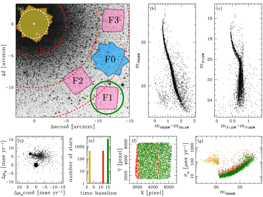
Figure 1: (a) Outlines of the fields of GO-14118 + GO-14662 data, superimposed on a DSS image of $\omega$ Cen. Units are in arcmin with respect to the cluster’s center. The primary ACS/WFC field (F0) is in azure, while the three parallel WFC3 fields are in pink. The data discussed in this paper come from field F1, which is highlighted by a green circle. We also show, in yellow, the central field of Bellini et al. (2017a). The white and red dashed circles mark the core radius ($r_{\rm c}$), the half-light radius ($r_{\rm h}$), $2\times r_{\rm h}$ and $3\times r_{\rm h}$ from the center outward, respectively. (b) The $m_{\rm F606W}$ versus $m_{\rm F606W}-m_{\rm F814W}$ CMD of sources with measured PMs. (c) The $m_{\rm F110W}$ versus $m_{\rm F110W}-m_{\rm F160W}$ CMD for the same sources. (d) The PM diagram, in units of ${\rm mas}\,{\rm yr}^{-1}$. Proper motions are measured relative to the bulk motion of the cluster. Cluster members are gathered together around (0,0). The lesser clump of points at around (+3.5,+6.5) is mainly background galaxies, and will be the subject of the next paper in this series (Libralato et al. 2018). (e) Histogram of the temporal baseline used to compute the PM of each source. Bright stars are unsaturated only in the short exposures of the third and fourth epochs, so that their PM is based on a temporal baseline of just two years (yellow bar). The longer temporal baseline ($\sim 15.1$ yr, green bar) is based on observations taken in at least the first and the fourth epochs. Sources outside the first-epoch FoV but measured in the remaining epochs have a temporal baseline of $\sim 11.7$ yr (red bar). (f) The master frame, in units of WFC3/UVIS pixels (40 mas pixel^-1). Sources are color-coded according to the temporal baseline used to measure their PM. (g) Proper-motion errors as a function of the $m_{\rm F606W}$ magnitude, color-coded as in panels (e) and (f). Well-measured stars in the long exposures have typical PM errors of about 10 $\mu$as yr^-1.

2 Data set and reduction

Field F1 has been observed a total of four times by HST. Long ACS/WFC observations in F606W and F814W were taken during the first two visits, in July 2002 (GO-9444) and in December 2005 (GO-10101). More recently, as part of our HST large program, the field was re-observed in August 2015 (GO-14118) and August 2017 (GO-14662), using both channels of the WFC3. In each of these two recent epochs, UVIS filters F275W, F336W, F438W (the so-called “magic trio”, e.g., Piotto et al. 2015), F606W and F814W, and IR filters F110W and F160W were utilized. The complete list of HST observations of field F1 is reported in Table 1. A link to the data is provided here: http://dx.doi.org/10.17909/T9FD49 (catalog 10.17909/T9FD49).

Panel (a) of Fig. 1 shows the location of the footprints of the GO-14118 and GO-14662 fields (F0 to F3) with respect to the center of the cluster (white cross), superimposed on a DSS image. Coordinates in arcmin with respect to the cluster’s center as measured by Anderson & van der Marel (2010): (R.A.,Dec.) = (13^h26^m47.$\!\!{}^{\rm s}$24,$-$47^∘28^′46$\farcs$45). The primary ACS/WFC field (F0) is in azure, while the three parallel WFC3 fields are in pink. As a reference, we also show the central field (in yellow) analyzed in Bellini et al. (2017a, b, c). The cluster’s core ($r_{\rm c}=1\farcm 31$) and half-light ($r_{\rm h}=2\farcm 37$) radii are marked with white and red dashed circles, respectively. The two outer red circles have a radius of $2\times r_{\rm h}$ and $3\times r_{\rm h}$, respectively. GO-14118 and GO-14662 fields cover a radial extent from $\sim 2\times r_{\rm h}$ to $\sim 4\times r_{\rm h}$. This paper focuses on field F1 (encircled in green), which is the only field for which all exposures have already been acquired.

The astro-photometric catalogs obtained in Milone et al. (2017b, hereafter, Paper I) for field F1 were constructed from the onset with the goal of detecting fine substructures on the color-magnitude diagram (CMD). Here our goal is to measure fine substructures on the PM diagram. Photometry and astrometry make very different demands on PSF analysis, with photometry more focused on sums of pixels, whereas for astrometry differences between nearby pixel values are key. A good PSF model should measure both fluxes and positions well, and our state-of-the-art reduction techniques allow just that. However, measurements that might end up being discarded because of high-precision photometric needs might still be useful for high-precision astrometric investigations, and vice versa. Selection procedures play a crucial role in obtaining appropriate stellar samples for astrometric or photometric studies, and there is generally no one-size-fits-all solution. For these reasons, we reduced all of the available exposures of field F1 from scratch, with the goal of high-precision astrometry right from the start. We will still make use of the photometry of Paper I (Sects 3 and 4) to isolate the mPOPs of the cluster.

Our astrometric and photometric reduction of the data set closely followed the procedures described in detail in Bellini et al. (2014) and in Bellini et al. (2017a), respectively. Below we provide a brief, general description of the entire reduction process, and emphasize the few important differences and fine tuning that we had applied to the Bellini et al. (2014) and Bellini et al. (2017a) procedures. We refer the interested reader to the original publications for an in-depth data-reduction description.

2.1 First-pass photometry

All ACS/WFC and WFC3/UVIS _flt exposures were pipeline-corrected to minimize the loss of charge-transfer efficiency (CTE), by means of the empirical pixel-based CTE correction described in Anderson & Bedin (2010). The WFC3/IR detector is based on a different read-out architecture, and it is not affected by CTE losses.

Next, we derived spatially-variable perturbation PSF models for each exposure, based on the few hundreds of bright, isolated, unsaturated stars within. The perturbation models were then combined to the spatially-variable—but time constant—empirical PSF libraries (e.g., Anderson & King 2006) to account for telescope breathing effects (Di Nino et al. 2008). These image-tailored PSF models were then used to measure stellar positions and fluxes in each exposure using the FORTRAN code hst1pass, which is an advanced version of the family of camera-dependent HST codes based on the img2xym_WFC software package (Anderson & King 2006). The routine hst1pass run a single pass of source finding for each exposure, and does not perform neighbor subtraction. The code then applies the appropriate camera-dependent reduction routines. Stellar positions in each single-exposure catalog (thereafter, first-pass catalog) were corrected using the state-of-the art geometric-distortion corrections of Anderson & King (2006, ACS/WFC), Bellini & Bedin (2009, WFC3/UVIS); Bellini et al. (2011, WFC3/UVIS), and the publicly-available WFC3/IR correction developed by J. Anderson.

2.2 The master frame

We cross-matched unsaturated stars in our first-pass catalogs with those in the Gaia data release 1 (DR1, Gaia Collaboration et al. 2016a, b) within 3 arcmin from the center of field F1. We found 131 sources in common, which were used as a reference to: (1) register our stellar positions to the Gaia-DR1 absolute astrometric system; and (2) define a right-handed, pixel-based, Cartesian reference frame (the master frame) with the X and Y axes parallel to the R.A. and Dec. directions, respectively, and with a pixel scale of exactly 40 ${\rm mas}\,{\rm pixel}^{-1}$(nearly the same as that of the WFC3/UVIS).

Then, we applied general, six-parameter linear transformations to transform the stellar positions of each first-pass catalog into the master frame, with which we created preliminary epoch- and filter-dependent average catalogs of positions and fluxes. The instrumental average photometry of these preliminary catalogs was obtained by rescaling the fluxes of each exposure to the instrumental magnitude zero-point of the first long exposure taken in each filter/epoch. The linear transformations we applied are based on likely $\omega$ Cen members on the basis of their positions on the instrumental F606W versus F606W$-$F814W CMD, so as to minimize large positional residuals due to stellar PMs of field stars over $\sim 15.1$ years.

2.3 Second-pass photometry

The FORTRAN software package KS2 (Anderson in preparation, see Bellini et al. 2017a for details) allows us to simultaneously measure stars in all the individual exposures and for the entire set of filters. KS2 is the evolution of kitchen_sync, originally designed to reduce specific ACS/WFC data (Anderson et al. 2008). KS2 takes the results of the first-pass photometry and the information coming from the six-parameter transformations into the master frame, and uses all the exposures together to find, measure, and subtract stars in several waves of finding, moving progressively from the brightest to the faintest stars. We closely followed most of the reduction prescriptions given in Bellini et al. (2017a), but we also applied a few critical changes (described below) aimed at maximizing the astrometric precision of the reduction.

KS2 is designed to work best in moderately crowded fields, so that it is limited by design to a 2-pixel search radius around the peak defined by each source on the master frame. Because we expect a significant fraction of field objects to have moved by more than 2 pixels (80 mas) over $\sim 15.1$ years with respect to the mean motion of the cluster, we decided to run KS2 over two distinct sets of data: GO-9444 and GO-10101 data (taken in 2002 and in 2005), GO-14118 and GO-14662 data (taken in 2015 and 2017). Both runs have long F606W and F814W exposures, so the finding stage of KS2 is based on these. This choice maximizes the number of common sources found in the two runs. Both KS2 runs performed nine finding passes, which allowed us to find and measure stars down to near the cluster’s hydrogen-burning limit (HBL).

KS2 measures stars in three different ways. The first method (method 1) applies when a star is bright enough to generate a distinct peak within its central $5\times 5$-pixel, neighbor-subtracted raster. In this case, KS2 measures the position and the flux of this star using the appropriate PSF model for the star’s location in an exposure. The other two methods do not fit stellar positions in each exposure, but rely on the positions determined during the finding stage. Although method 1 does not allow us to obtain photometry of stars as faint as those recovered by methods 2 and 3, method 1 is the only method for which stellar positions are solved for in each individual exposure. As such, for the remainder of this paper, we will consider only stellar positions as measured by the KS2 method 1.

In addition to the photometric diagnostics described in Bellini et al. (2017a), we also had KS2 output the RADXS parameter (Bedin et al. 2008). RADXS tells us how much flux a source has with respect to the PSF predictions just outside the PSF core. Galaxies and blends have large positive values of RADXS, while objects sharper than the PSF, e.g. cosmic rays or hot pixels, have large negative values of RADXS.

KS2 found a total of 28 345 sources in the first run based on ACS/WFC exposures, and 14 883 sources in the second run based on WFC3 exposures, due to the smaller field of view (FoV) of the latter data set. In both cases, sources are measured in both F606W and F814W filters. We cross-identified the objects in these two lists and found 8751 sources measured in all four epochs. These sources constitute the master list that we will use in Sect. 2.5 to compute PMs.

2.4 Photometric calibration

Instrumental magnitudes were zero-pointed to the Vega-mag flight system following the prescriptions given in Bellini et al. (2017a). We employed a radius of $0\farcs 4$ (10 pixels on the master frame) for the aperture photometry on the HST-pipeline-calibrated _drc and _drz images. The adopted ACS/WFC Vega-mag zero points are from Bohlin (2016). For the WFC3 filters, Vega-mag zero points are available at the official WFC3 zero-point website.

Panels (b) and (c) of Fig. 1 show the visual $m_{\rm F606W}$ versus $m_{\rm F606W}-m_{\rm F814W}$ and the IR $m_{\rm F110W}$ versus $m_{\rm F110W}-m_{\rm F160W}$ CMDs of the 8751 sources measured in all four epochs. Saturation in the long F606W exposures starts at $m_{\rm F606W}\approx 20.4$. Photometry of brighter stars is based only on the short exposures (four per filter) of GO-14118 and GO-14662.

2.5 Proper-motion measurements

As shown in Bellini et al. (2011), filters bluer than F336W are not suitable for high-precision astrometry, because of the presence of color-dependent residuals in the UVIS distortion solution. Therefore, F275W exposures were not used to compute high-precision PMs.

Unlike the case of WFC3/UVIS and ACS/WFC detectors (Bellini et al. 2014), the characterization of systematic effects possibly affecting astrometry in the WFC3/IR has just begun (e.g., Zhou et al. 2017). In addition, the WFC3/IR detector suffers from a more severe undersampling of the PSF and has a significantly larger pixel scale ($0\farcs 13$ pixel^-1) with respect to both the WFC3/UVIS ($0\farcs 04$ pixel^-1) and ACS/WFC ($0\farcs 05$ pixel^-1). We initially included WFC3/IR exposures to compute PMs, but we found negligible improvements in terms of PM errors and number of measured sources with respect to using only WFC and UVIS exposures. Therefore, for this particular study, IR exposures were not included in the analysis.

Proper motions are computed by closely following the procedures described in detail in Bellini et al. (2014), in which each individual exposure is treated as a stand-alone epoch, and PMs are iteratively obtained as the slope of the straight-line fits to the master-frame stellar positions versus epoch of observation. The main process is divided into five steps: (1) measure stellar positions in each exposure; (2) define/improve a common master list based on a set of reference stars at a specific epoch; (3) cross-identify stars measured in different exposures with those in the master list; (4) transform the (X,Y) position of each star as measured in all the exposures where the star is found on to the master frame, using a local network of reference stars; (5) fit straight lines to the master-frame transformed positions versus epoch. The slope of the fit provides a direct measurement of the PM.

We already have all the necessary pieces of information for step (1). Unlike Bellini et al. (2014), which made use of stellar positions as measured by the first-pass photometry, here we started from the stellar positions measured by KS2 method 1. KS2 offers a significant advantage over the first-pass photometry, since it deblends each source prior to fitting of the PSF. Steps (2), (3), (4), and (5) are nested into each other, and each of them is iterated in order to: (i) allow for the rejection of discrepant observations; and (ii) improve the reference star list, the master-frame transformations, and the PM measurements themselves.

As a common reference frame we started with the Gaia-based master frame defined in Sect. 2.2. We also defined an initial set of likely cluster members (the reference stars) extracted from the master list on the basis of their location on the CMD. Steps (2) to (5) are iterated as detailed in Bellini et al. (2014). At the end of each iteration, the list of reference stars is improved by removing all objects for which the PM is not consistent with the cluster’s mean motion.

Figure 2: From left to right, $m_{\rm F606W}$ versus $F-m_{\rm F814W}$ CMDs, with $F$ increasing from $m_{\rm F275W}$ to $m_{\rm F606W}$, respectively. Each CMD shows only PM-selected cluster members. The horizontal line represents the saturation level in long GO-14118 and GO-14662 exposures. Stars brighter than this line have PMs obtained over a temporal baseline of just two years. Fainter stars have PMs computed over temporal baselines of at least 11.7 years.

For each star $i$ in each exposure, position transformations on to the master frame are typically based on the subset of reference stars (typically a few hundreds) that are within the same detector amplifier of the star $i$ (to minimize the impact of uncorrected geometric-distortion and CTE-mitigation residuals). Only at the last iteration we further restrict the subset of reference stars to the closest 45 to the star $i$ (the so-called local transformations, e.g., Anderson et al. 2006).

Proper-motion fitting and data rejection are performed exactly as described in Bellini et al. (2014). Briefly, for each star we fit all the transformed X and Y positions coming from different exposures as a function of the exposure epoch by means of a least-squares straight line. After obvious outliers have been rejected, the residuals of the fit of both X and Y positions are collected together and rescaled so that, to the lowest order, their distribution should be consistent with a two-dimensional Gaussian. We iteratively rejected one data point at a time if its combined residuals are consistent with a two-dimensional Gaussian distribution to less than 2.5% confidence level (see Sect. 5.5 of Bellini et al. 2014 for more details).

Because of the large internal velocity dispersion of $\omega$ Cen in field F1 ($\sim 0.34$ ${\rm mas}\,{\rm yr}^{-1}$), cluster stars have moved on average by about 0.13 pixels between 2002 and 2017. Field objects have moved on average much more than that, $\gtrsim 2.5$ pixels, forcing us to allow for a generous search radius (5 pixels) to cross-identify stars of each exposure with the master list. This inevitably led to some misidentifications. At the end of the first iteration, PMs can be used to estimate the master list positions at the precise epoch of each exposure. This allowed us to adopt a much tighter search radius (0.75 pixels) to minimize the inclusion of false positives. Moreover, we redefined the master list so that the position of its sources is referred to the average epoch of the data (the reference epoch): 2010.42285. We iterated steps (2) to (5) a few more times, until the predicted master-list positions at the reference epoch changed by less than 0.001 pixel and the number of reference stars remains constant from one iteration to the next.

The initial master list contained 8751 sources, but we were able to compute high-precision PMs for only 5153 sources. The missing 3598 sources were rejected during the various PM-measurement iterations according to a variety of different reasons, all related to data quality and self consistency. All rejection criteria are listed and described in Bellini et al. (2014). Our final PM catalog is supplied with the same set of quality and diagnostic parameters described in Bellini et al. (2014).

Panel (d) of Fig. 1 shows the PM diagram of the 5153 measured sources. Because our reference list consists of cluster members, our PMs are relative to the bulk motion of the cluster, and cluster members are gathered together around (0,0). The lesser clump of sources at about (+3.5,+6.5) is mostly populated by background galaxies, and will be the subject of the next paper in this series (Libralato et al. 2018). All other sources are foreground and background field stars. Note that we refer to $\Delta\mu_{\alpha}\cos\delta$ and $\Delta\mu_{\delta}$ PM components, rather than $\mu_{\alpha}\cos\delta$ and $\mu_{\delta}$, because we want to emphasize the fact that our PMs are relative to the cluster’s mean motion.

Panel (e) shows the distribution of the temporal baselines used to compute the PM of each star. Because stars brighter than $m_{\rm F606W}\sim 20.4$ are unsaturated only in the (few) short exposures of GO-14118 and GO-14662, their PM is based on a temporal baseline of just $\sim 2$ years (yellow). The vast majority of the remaining stars are measured in all four epochs, providing a temporal baseline of $\sim 15.1$ years (green). Finally, sources outside the GO-9444 FoV but measured in the other three epochs have PMs computed over a temporal baseline of $\sim 11.7$ years (red). The (X,Y) position of sources with measured PMs are shown on the pixel-based master frame in panel (f), color-coded according to the relevant temporal baseline used to compute their PM. Finally, PM errors as a function of the $m_{\rm F606W}$ magnitude are in panel (g), also color-coded according to the temporal baseline used. Clearly, the PM error of bright stars (yellow) is significantly larger than that of faint stars, which are based on much longer temporal baselines and larger number of images. Well-measured stars in the long exposures ($20.4\lesssim m_{\rm F606W}\lesssim 22.4$) have PM errors of about 10 $\mu$as yr^-1. (Note that Gaia’s expected end-of-mission PM precision at the faint limit ($\gtrsim 0.9$ mas yr^-1 at $m_{\rm F606W}\sim 21.5$) is over a factor of 90 worse, Pancino et al. 2017).

Exposures taken with the magic trio of filters (F275W, F336W and F438W) are significantly shallower than those taken with the F606W and the F814W. This can be clearly seen in Fig. 2, in which we plot four different CMDs of the form $m_{\rm F814W}$ versus $F-m_{F814W}$, with $F$ varying from F275W to F606W from the left to the right panels. In all panels, only stars whose motion is within 1.5 ${\rm mas}\,{\rm yr}^{-1}$ of the cluster’s mean motion are shown. The F606W saturation level in the long exposures is marked in all panels. Clearly, F275W exposures are the least complete.

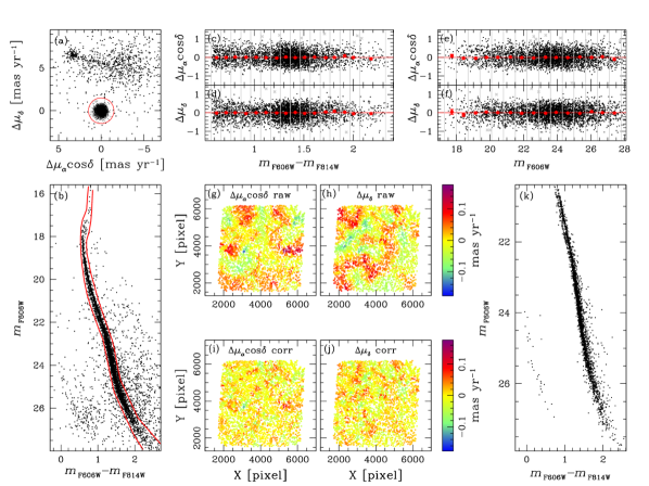
Figure 3: This figure illustrates the a-posteriori correction procedures applied to the raw PM measurements. (a) PM diagram of the sources in field F1. We preliminary select cluster members as all objects within the red circle of radius 1.5 ${\rm mas}\,{\rm yr}^{-1}$. (b) An additional selection makes use of stellar positions on the $m_{\rm F606W}$ versus $m_{\rm F606W}-m_{\rm F814W}$ CMD (within the two red lines drawn by hand). Panels (c) and (d) show that raw PMs do not suffer from systematic effects as a function of stellar color. Similarly, panels (e) and (f) show that raw PMs do not suffer from systematic effects as a function of stellar magnitude. Note that the horizontal red lines at $\Delta\mu=0$ in these four panels are not a fit to the data, but indicate lack of trends. In panels (g) and (h) we report the maps of the locally-measured (closest 100 stars) mean raw PM components of cluster members. Specifically, the deviation along $\mu_{\alpha}\cos\delta$ is in panel (g), and the deviation along $\mu_{\delta}$ is in panels (g) and (h). Each star is color-coded according as shown by the vertical bar the immediate right of panel (h). Panels (i) and (j) show the maps of the locally-measured mean corrected PM of cluster members. We applied the same color-scheme as in panels (g) and (h). Finally, panel (k) shows the $m_{\rm F606W}$ versus $m_{\rm F606W}-m_{\rm F814W}$ CMD of cluster members with high-quality PMs. See the text for details.

2.6 Proper-motion corrections

Following the prescriptions given in Bellini et al. (2014, their Sects. 7.3 and 7.4) we applied a-posteriori corrections to mitigate any residual source of systematic errors. We started by selecting likely cluster members on the basis of their position on the PM diagram (within 1.5 ${\rm mas}\,{\rm yr}^{-1}$ from the bulk distribution, red circle in panel (a) of Fig. 3) and of their position on the $m_{\rm F606W}$ versus $m_{\rm F606W}-m_{\rm F814W}$ CMD (within the two red lines shown in panel (b) of the same figure).

We verified that neither component of the PM suffers from systematic effects due to stellar color (panels c and d) and luminosity (panels e and f). In each of these panels, we divided the sample into equally populated bins in color or in magnitude (within the gray vertical lines). Within each bin, we computed the 3$\sigma$-clipped median value of the motion along $\Delta\mu_{\alpha}\cos\delta$ and $\Delta\mu_{\delta}$. Rejected stars are shown with gray crosses. The computed median values are shown as red solid circles, with errorbars. The associated errors of the mean are typically smaller than the size of red circles. The horizontal red line is not a fit to the data, but indicates lack of systematic effects. It is clear from panels (c), (d), (e), and (f) that color and luminosity systematic effects, if present, are negligible.

We did notice marginal, spatially-varying systematic effects as a function of stellar positions on the master frame. These spatial effects are due to small single-exposure CTE and geometric-distortion residuals that, given the relative small number of different roll angles employed (up to three), do not cancel out. These effects can be divided into a low- and a high-frequency variation. The low-frequency variation correlates well with the map of the temporal baseline used to compute PMs, which in turn reflects the number and type of overlapping images at any given location on the master frame. We corrected this systematic effect by computing three median values of each component of the motion of selected cluster members, one for each of the three groups of temporal baselines shown if Fig. 1e, and subtracting them from the motion of each star according to the temporal baseline used. By construction, these median values should all be equal to zero. Instead, we found deviations of the order of a few tens of $\mu$as yr^-1 (note that the measured cluster dispersion is much larger, about $\sim 0.34$ mas yr^-1).

High-frequency-variation systematic effects were corrected as described in Sect. 7.4 of Bellini et al. (2014). In a brief, both components of the motion of each star were corrected according to the median value of the closest 100 likely cluster members (excluding the target star itself). Again, by construction the median should be equal to zero, and the measured deviation is used as the local correction. Note that here local corrections are only based on distance and not on magnitude, as it was the case in Bellini et al. (2014), because our PMs do not suffer from systematic effects due to stellar color or magnitude (panels (c), (d), (e) and (f) of Fig. 3).

Panels (g) and (h) of Fig. 3 show the maps of the local median values obtained with the uncorrected (raw) components of the motion; $\Delta\mu_{\alpha}\cos\delta$ in panel (g) and $\Delta\mu_{\delta}$ in panel (h). Each point is a source, color-coded according its locally-averaged PM value, as shown on the color bar on the right-hand side of panel (g). Panels (i) and (j) show similar maps after the high-frequency variations are corrected. Points are color-coded using the same color scheme as panels (g) and (h). The overall size of the local PM variations is significantly lower than those of the uncorrected maps. The uncorrected maps have a root mean square (RMS) of 42 $\mu$as yr^-1. The RMS of the corrected maps is 27 $\mu$as yr^-1 (i.e., about 8% of the intrinsic velocity dispersion of the cluster).

Both the low-frequency and the high-frequency a-posteriori corrections come at a cost. In fact, the corrections we applied to each star are based on the median value of a sample of cluster members, which have their own intrinsic dispersion. As a result, there is an error associated to these corrections, i.e., the standard error of the mean. For instance, the high-frequency variations were corrected using the median motion of 100 stars, so that the associated error is of the order of $\sim 0.34/\sqrt{100}\,{\rm mas}\,{\rm yr}^{-1}\sim 34\,\mu{\rm as}\,{\rm yr}^{-1}$ per coordinate. Similar (but smaller, due to the larger sample size) correction errors are found for the low-frequency variation. The effects of the increased PM errors are reflected in a marginally larger (but rounder) cluster dispersion on the PM diagram. The total PM errors associated to the a-posteriori corrected PMs are the sum in quadrature of the raw PM errors and both the low- and high-frequency correction errors. Since different scientific investigations favor the use of one or the other way of estimating PMs, our final PM catalog contains both the raw and the corrected PMs, with uncertainties (see Sect.A).

2.7 Proper-motion selections

We aim to study the finest kinematic details of the mPOPs of the cluster, so we applied a few selection criteria to our PM catalog in order to analyze the best measured sources. To start, we selected only stars for which the computed PM is based on the longest available temporal baseline ($\sim 15.1$ yr). In addition, we restricted the sample to stars that are: (1) measured in at least 10 distinct exposures; (2) with a rejection rate of less than 15%, (3) with reduced $\chi^{2}<4$ in each coordinate; (4) with fluxes above $3\sigma$ the local sky background; (5) with RADXS values in F606W and F814W between $-0.05$ and 0.05; (6) QFIT values in F606W and F814W greater than 0.7; and (7) with PMs within 1.5 ${\rm mas}\,{\rm yr}^{-1}$with respect to the cluster’s bulk motion, a value $\sim 4.5$ times larger than the observed cluster dispersion. With this initial list, we iteratively rejected stars with PM errors larger than 50% of the local velocity dispersion, as described in Sect. 7.5 of Bellini et al. (2014).

These selection procedures were applied to both the raw and the corrected PMs, and we run a parallel analysis on both sets of PM measurements. The resulting velocity-dispersion profiles for the raw and the corrected PM measurements were consistent with each other well within the uncertainties. In what follows, we present the analysis on the kinematics of the mPOPs of the cluster based on corrected PM measurements. The final list of high-precision, PM-selected cluster members includes 2912 sources, extending from $m_{\rm F606W}\simeq 20.4$ down to near the HBL at $m_{\rm F606W}\sim 28$. Panel (k) of Fig. 3 shows the $m_{\rm F606W}$ versus $m_{\rm F606W}-m_{\rm F814W}$ CMD of these 2912 cluster stars.

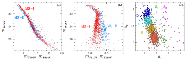
Figure 4: (a) MS-I (red) and MS-II (azure) stars on the $m_{\rm F606W}$ versus $m_{\rm F606W}-m_{\rm F814W}$ CMD. (b) MS-I and MS-II stars on the $m_{\rm F606W}$ versus $m_{\rm F110W}-m_{\rm F160W}$ CMD. (c) The $\Delta_{2}$ versus $\Delta_{1}$ chromosome map (see Paper I) with the six populations identified below the MS knee. The four main populations are: A (orange), B (yellow), C (cyan) and D (blue). The two lesser subgroups are S₁ (green) and S₂ (magenta). All populations are selected as in Paper I. See the text for details.

3 Multiple-population kinematics

3.1 Naming conventions

The MS of $\omega$ Cen has been known for 20 years to be split into two main components (e.g., Anderson 1997; Bedin et al. 2004), which were historically named the blue MS (bMS) and the red MS (rMS), and a lesser, “anomalous” component (MSa) associated with the peak of the [Fe/H] distribution. Hints of an even more complicated scenario were discovered by Bellini et al. (2010), in which both the rMS and the MSa turned out to be themselves split into two subcomponents.

More recently, thanks to the same five UVIS filters used in this large program, distinct mPOPs have been detected in all the GCs analyzed so far, including $\omega$ Cen (see, e.g., Piotto et al. 2015; Bellini et al. 2017c; Milone et al. 2017a, and references therein). In particular, the latter authors identified up to 17 populations on the RGB, with each of them possibly related to distinct Fe, O, and Na abundances (Marino et al. 2011). At the bright MS level, Bellini et al. (2017c) isolated at least 15 distinct MS populations in the cluster core, organized into 5 main population groups, which they named as: rMS, bMS, MSd, MSe, and MSa. (Please note that the rMS and the bMS defined in Bellini et al. 2017c are actually subcomponents of the historical rMS and bMS, respectively.)

In particular, the rMS, the bMS, and the MSd groups as defined in Bellini et al. (2017c) are each split into three subcomponents (e.g., the rMS is made up of rMS1, rMS2, and rMS3 subpopulations); the MSe is made up of four subcomponents, while MSa is divided into two subcomponents. Both the bMS and the MSd groups are consistent with stellar populations being highly enriched in He and moderately enriched in Fe with respect to the rMS group. The MSe group, on the other hand, shares similar properties to the rMS. Finally, both MSa subpopulations are likely highly enriched in both He and Fe.

Since both the historical rMS and bMS populations are actually made up of several population subgroups, in Paper I we decided to use the labels MS-I and MS-II, respectively, to refer to these two main MS branches that can be seen on a visual CMD. In addition, in Paper I we also made use of the IR filters F110W and F160W to identify for the first time four main groups of stars below the MS knee, which we named as populations A, B, C, and D, plus two lesser MS components that we called populations S₁ and S₂. These populations merge together in the proximity of the MS knee, and above the knee only the MS-I and MS-II meta-groups can be identified using IR filters and/or visual filters.

Clearly, there is quite some room for confusion with population names. To complicate things, different authors have used different names to refer to same populations of $\omega$ Cen, especially along the RGB. In what follows, we will adopt the meta-group naming convention of Paper I. We will also use the terms first-generation (1G) and second-generation (2G) stars to refer to the stars of the meta-groups MS-I and MS-II, respectively, to emphasize differences in their dynamical-evolution histories. 1G stars in $\omega$ Cen are characterized by primordial (or at most slightly-enhanced) He abundance, and are generally metal poor. 2G stars are highly He enhanced and are metal rich. Clear hints of dynamical differences between 1G and 2G stars in the cluster have been found by studying their radial distribution (Sollima et al. 2007; Bellini et al. 2009a), with 2G significantly more centrally concentrated than 1G stars.

Finally, we will use the same labels of Paper I for the six population groups identified below the MS knee using IR photometry, and the same names of Bellini et al. (2017c) for the five population groups identified on the bright MS using UV photometry.

3.2 Subpopulation selections

As we can see in Fig. 2, the photometry obtained with the magic trio of filters in our field F1 is dramatically shallow (especially in F275W), to the point where no meaningful kinematic properties can be derived if we use them to isolate the different mPOPs of the cluster, as done in Bellini et al. (2017c). Therefore, we applied the same selection criteria of Paper I (as well as the high-quality photometry of Paper I) to isolate stars in the MS-I and MS-II meta-groups, as well as in the six populations below the MS knee.

Panels (a) and (b) of Fig. 4 show MS-I (1135 stars, red) and MS-II stars (385 stars, azure), as defined in Paper I, on the $m_{\rm F606W}$ versus $m_{\rm F606W}-m_{\rm F814W}$ and on the $m_{\rm F606W}$ versus $m_{\rm F110W}-m_{\rm F160W}$ CMDs, respectively. The $\Delta_{2}$ versus $\Delta_{1}$ chromosome map of stars below the MS knee is in panel (c), with the six populations identified and color-coded as in Paper I: A (523 stars, orange), B (202 stars, yellow), C (117 stars, cyan), D (133 stars, blue), S₁ (36 stars, green), and S₂ (25 stars, magenta). We refer the reader to Paper I for a detailed description of the population selections. All stars plotted in Fig 4 have high-precision PM measurements.

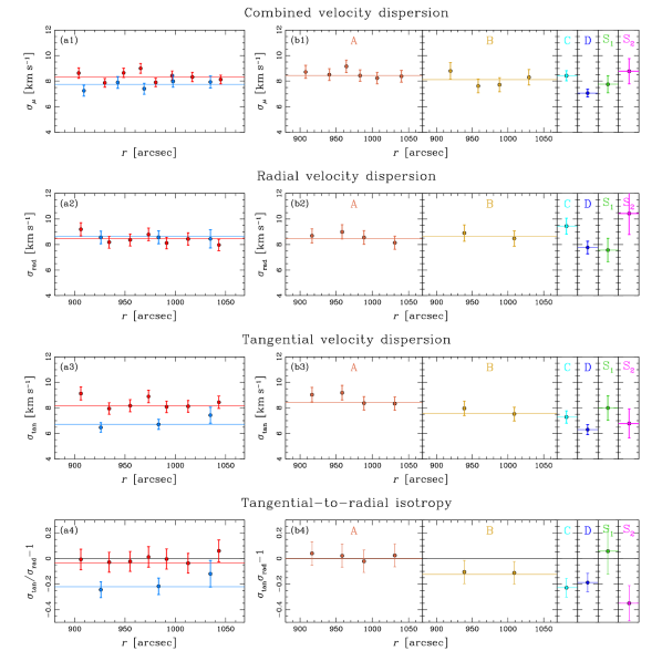
Figure 5: (a1) velocity dispersion $\sigma_{\mu}$ as a function of the distance from the cluster’s center, $r$, for MS-I (red) and MS-II (azure) stars. (b1) $\sigma_{\mu}$ versus $r$ for the six populations below the MS knee. From left to right: A, B, C, D, S₁, and S₂, respectively. Populations are color-coded as in Fig. 4. Because of low-number statistics, the combined velocity dispersion of populations C, D, S₁, and S₂ is computed over the entire FoV. (a2) and (b2) are similar to (a1) and (b1) but for $\sigma_{\rm rad}$, the radial component of the velocity dispersion. (a3) and (b3) are for the tangential component of the velocity dispersion $\sigma_{\rm tan}$. (a4) and (b4) show the deviation from tangential-to-radial isotropy. See the text for details.

3.3 Velocity-dispersion profiles

Velocity dispersions are estimated using the same method described in van der Marel & Anderson (2010), which corrects the observed scatter for the individual stellar PM uncertainties. Unless stated otherwise, we indicate with $\sigma_{\mu}$ the average one-dimensional velocity dispersion of the combined $\Delta\mu_{\alpha}\cos\delta$ and $\Delta\mu_{\delta}$ PM components. We do not expect significant differences in the velocity dispersion as a function of distance from the cluster center within the field F1, because of the relatively small field size compared to its distance from the cluster center. Nevertheless, for those populations with at least 200 stars, namely: MS-I, MS-II, A, and B, we measured $\sigma_{\mu}$ in equally-populated radial intervals. For the remaining populations C, D, S₁, and S₂ we derived a single value of the velocity dispersion over the entire field. Velocity dispersions are given in units of ${\rm km}\,{\rm s}^{-1}$ by assuming a cluster distance of 5.2 kpc (Harris 1996).

Panel (a1) of Fig. 5 shows the velocity-dispersion profiles $\sigma_{\mu}$ of the MS-I (red) and MS-II (azure) meta-groups as a function of the distance from the cluster center. The horizontal red (MS-I) and azure (MS-II) lines mark the average $\sigma_{\mu}$ value computed over the entire field, and are not the average of the $\sigma_{\mu}$ values of the radial bins. Both meta-groups show a flat distribution of $\sigma_{\mu}$ versus radius. MS-II (2G) stars appear to be slightly kinematically colder than MS-I (1G) stars. The average velocity dispersion of both MS-I and MS-II stars, about 8 ${\rm km}\,{\rm s}^{-1}$, is more than a factor of two less than in the central field (Anderson & van der Marel 2010), as a direct consequence of hydrostatic equilibrium (see also Bellini et al. 2014).

Panel (b1) of Fig. 5 shows the velocity-dispersion profiles for the six populations below the MS knee. For clarity, profiles of different populations are shown separately, from population A to population S₂ from the left to the right, respectively. The average $\sigma_{\mu}$ values of the populations computed over the entire field (colored horizontal lines) are all consistent with each other within the errors, except for population D. We find population D to be significantly kinematically colder than population A at the 3$\sigma$ confidence level. It is worth to stress that no radial dependence of the velocity dispersion is present in the analyzed field.

Panels (a2) and (b2) are similar to panels (a1) and (b1) but for the velocity dispersion of the radial (i.e., towards the center of the cluster, not along the line of sight) component of the motion $\sigma_{\rm rad}$. We find MS-I and MS-II to have the same radial velocity dispersion. Similarly, we find all of the six populations in (b2) to have the same radial velocity dispersion within the errors. In panels (a3) and (b3) we report the velocity-dispersion profiles of the tangential component of the motion ($\sigma_{\rm tan}$) for each population. The $\sigma_{\rm tan}$ of the MS-II meta-group is significantly lower, at the 3.2$\sigma$ level, than that of the MS-I. Below the MS knee we find the average $\sigma_{\rm tan}$ of populations B, C, and D to be progressively lower (and with increasing confidence level) than that of population A.

The average values of $\sigma_{\mu}$, $\sigma_{\rm rad}$, and $\sigma_{\rm tan}$ for each population, with associated errors, are listed in Table 2.

Table 2: Multiple-population kinematics in field F1.

Population	$N_{\rm stars}$	$\sigma_{\mu}$	$\sigma_{\rm rad}$	$\sigma_{\rm tan}$	$\sigma_{\rm tan}/\sigma_{\rm rad}-1$	$\langle\mu_{\alpha}\cos\delta\rangle$	$\langle\mu_{\delta}\rangle$	$\langle\mu_{\rm rad}\rangle$	$\langle\mu_{\rm tan}\rangle$
		(${\rm km}\,{\rm s}^{-1}$)	(${\rm km}\,{\rm s}^{-1}$)	(${\rm km}\,{\rm s}^{-1}$)		(${\rm mas}\,{\rm yr}^{-1}$)	(${\rm mas}\,{\rm yr}^{-1}$)	(${\rm mas}\,{\rm yr}^{-1}$)	(${\rm mas}\,{\rm yr}^{-1}$)
MS-I	1135	$8.31\pm 0.13$	$8.46\pm 0.19$	$8.16\pm 0.18$	$-0.035\pm 0.031$	$-0.003\pm 0.010$	$0.033\pm 0.011$	$-0.022\pm 0.010$	$+0.024\pm 0.010$
MS-II	385	$7.73\pm 0.22$	$8.63\pm 0.34$	$6.71\pm 0.27$	$-0.222\pm 0.044$	$0.031\pm 0.016$	$-0.040\pm 0.016$	$0.022\pm 0.018$	$-0.064\pm 0.014$
A	523	$8.44\pm 0.15$	$8.45\pm 0.22$	$8.43\pm 0.22$	$-0.002\pm 0.036$	$0.011\pm 0.015$	$0.043\pm 0.016$	$-0.040\pm 0.015$	$+0.024\pm 0.016$
B	202	$8.12\pm 0.27$	$8.64\pm 0.40$	$7.57\pm 0.35$	$-0.125\pm 0.057$	$-0.010\pm 0.023$	$0.029\pm 0.024$	$-0.018\pm 0.025$	$+0.010\pm 0.022$
C	117	$8.43\pm 0.40$	$9.44\pm 0.63$	$7.28\pm 0.49$	$-0.229\pm 0.073$	$0.018\pm 0.030$	$-0.068\pm 0.033$	$0.085\pm 0.035$	$-0.108\pm 0.027$
D	133	$7.06\pm 0.31$	$7.77\pm 0.49$	$6.30\pm 0.40$	$-0.189\pm 0.072$	$0.059\pm 0.026$	$-0.016\pm 0.024$	$-0.029\pm 0.027$	$-0.033\pm 0.022$
S1	36	$7.76\pm 0.66$	$7.56\pm 0.91$	$8.00\pm 0.96$	$0.057\pm 0.18$	$-0.008\pm 0.048$	$0.103\pm 0.052$	$-0.065\pm 0.051$	$+0.173\pm 0.049$
S2	25	$8.77\pm 0.99$	$10.44\pm 1.6$	$6.78\pm 1.1$	$-0.35\pm 0.15$	$0.154\pm 0.087$	$0.029\pm 0.067$	$-0.189\pm 0.091$	$-0.098\pm 0.060$
WDs	29	$8.39\pm 0.88$	$8.98\pm 1.32$	$7.78\pm 1.17$	$-0.13\pm 0.18$	$0.108\pm 0.074$	$-0.097\pm 0.057$	$0.02\pm 0.10$	$-0.201\pm 0.088$

3.4 Anisotropy

Regardless of the exact mechanism(s) that led to the formation of mPOPs of stars in GCs (e.g., Decressin et al. 2007; D’Ercole et al. 2008; Bastian et al. 2013, but see Renzini et al. 2015 for a critical review), all models assume 2G (MS-II) stars to form more spatially concentrated than 1G (MS-I) stars. The subsequent long-term dynamical evolution of the cluster will eventually erase any difference in the spatial distributions of 1G and 2G stars. $N$-body simulations (e.g., Bellini et al. 2015a) show that 2G stars gradually diffuse from the cluster’s inner regions to the outskirts (which are initially dominated by 1G stars) preferentially on radial orbits. The outskirts of massive-enough clusters have local two-body-relaxation times long enough that we should still be able to see the fingerprints of the dynamical evolution of their mPOPs. Indeed, this has been observed in 47 Tuc (Richer et al. 2013) and in NGC 2808 (Bellini et al. 2015a). Both 47 Tuc ($\sim 1.3\times 10^{6}\,\mathrm{M}_{\odot}$, Heyl et al. 2017) and NGC 2808 ($\sim 1.4\times 10^{6}\,\mathrm{M}_{\odot}$, Boyles et al. 2011) are among the most massive GCs of the Milky Way, and the fields analyzed by Richer et al. (2013) and Bellini et al. (2015a) are outside $\sim 2\times r_{\rm h}$.

$\omega$ Cen is the most massive GC of the Galaxy, with an estimated mass of $\sim 4\times 10^{6}\,\mathrm{M}_{\odot}$ (D’Souza & Rix 2013), and our field F1 is located at $\sim 3\times r_{\rm h}$ from the center. Therefore, we do expect to detect significant differences in the internal kinematics between 1G and 2G stars, in particular in their velocity dispersion along the tangential direction. Indeed, this is exactly what we find (panels (a2), (a3), (b2), and (b3) for Fig. 5).

The deviation from tangential-to-radial isotropy (that is, the ratio between the velocity dispersions measured along the tangential and the radial directions minus one, or $\sigma_{\rm tan}$/$\sigma_{\rm rad}$$-$1) of the two MS meta-groups and of the six populations below the MS knee are shown in panels (a4) and (b4) of Fig. 5, respectively. In both panels, the black horizontal line marks full isotropy. We find MS-I stars to be consistent with being isotropic, while MS-II stars are significantly radially anisotropic (5$\sigma$ confidence level). Below the MS knee, populations A and S₁ are consistent with being fully isotropic, while populations B, C, D and S₂ appear to be radially anisotropic (at the 2.2$\sigma$, 3.1$\sigma$, 2.6$\sigma$, and 2.3$\sigma$ confidence levels, respectively).

According to the mPOP dynamical evolution models of Bellini et al. (2015a), the tangential velocity dispersion of 2G stars evolves towards smaller values than that of 1G stars, in agreement with our observations. It is the difference in $\sigma_{\rm tan}$ that is responsible for the differences in the anisotropy of 1G and 2G stars.

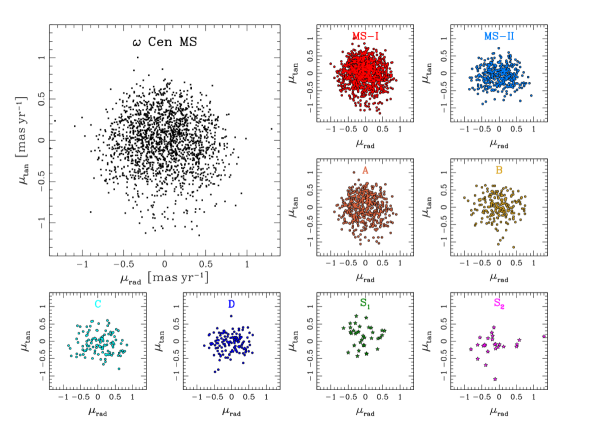
Figure 6: The main panel shows the distribution of MS stars in the $\mu_{\rm tan}$ versus $\mu_{\rm rad}$ plane. The smaller panels are similar but show the individual populations.

3.5 Differential rotation

First of all, we note that all the populations analyzed in this work have the baricenter of the motion very close to the origin of the PM diagram. We find the median value of the motion along the $\alpha\cos\delta$ direction, $\langle\mu_{\alpha}\cos\delta\rangle$, of each population to be consistent with zero with at most marginal deviations. However, a few small but significant (at the $\gtrsim 3$$\sigma$ level) deviations are present for MS-I, MS-II and population A stars along the $\delta$ direction. In all three cases, the median motion along the $\delta$ direction, $\langle\mu_{\delta}\rangle$, is of the order of 0.04 ${\rm mas}\,{\rm yr}^{-1}$ (or just about 1 ${\rm km}\,{\rm s}^{-1}$). (The $\langle\mu_{\alpha}\cos\delta\rangle$ and $\langle\mu_{\delta}\rangle$ values of each population are reported in Table 2.) Ferraro et al. (2002) combined the photographic-plate-based PM catalog of van Leeuwen et al. (2000) with the RGB photometry of Pancino et al. (2000), and found a much larger difference ($\sim 0.8$ ${\rm mas}\,{\rm yr}^{-1}$) between the relative PM of the RGBa population (evolved MSa stars) and the cluster’s bulk motion. The culprit of this large PM offset was discovered by Platais et al. (2003). The authors presented a detailed reanalysis of the van Leeuwen et al. (2000) PM catalog, and showed that it contains severe color/magnitude-induced systematic effects. No significant PM offsets between the different mPOPs of the clusters was later reported by Bellini et al. (2009b) for RGB stars, and by Anderson & van der Marel (2010) for bright MS stars in the core. Our PMs analysis of field F1 populations further support the absence of major PM deviations between the mPOPs of the cluster.

Analysis of the radial ($\mu_{\rm rad}$) and tangential ($\mu_{\rm tan}$) PM components provides a more qualitative way to estimate the deviation from tangential-to-radial isotropy of the mPOPs we found in the previous Section, as well as a better understanding of the nature of the small but significant deviation from zero of the relative bulk PM of MS-I, MS-II, and population A stars. As a reference, we show in the large panel of Fig. 6 the PM distribution of all $\omega$ Cen’s MS stars in the field along the tangential and radial components. The smaller panels are similar but show the individual populations. The MS-I and the population A distributions are visibly rounder than those of the MS-II and of populations B, C, D, and perhaps also S₂, which in turn are flattened along the $\mu_{\rm tan}$ direction. In addition, it appears that distribution of population S₁ is rounder than—say—the MS-II.

The large panel of Fig. 6 also reveals that MS distribution is somewhat skewed towards negative $\mu_{\rm tan}$ values. A similar behavior has also been recently reported for stars in an outer field of 47 Tuc (Heyl et al. 2017). The authors attribute the presence of the skew to differential rotation of stars in the field. 47 Tuc is characterized by a high clockwise rotation in the plane of the sky (see Bellini et al. 2017d), with a peak of the intrinsic rotational velocity over velocity dispersion $V/\sigma$ of $\sim 0.9$ at around two $r_{\rm h}$, which is where the outer field of Heyl et al. (2017) lies. Also the GC $\omega$ Cen is known to be rotating (counter-clockwise in this case) in the plane of the sky (e.g., van Leeuwen et al. 2000; van de Ven et al. 2006; Watkins et al. 2013), so the presence of skewness in the $\mu_{\rm tan}$ distribution should not come as a surprise. It is known from studies of elliptical galaxies that rotation is generally accompanied by skewness in the line-of-sight velocity distribution (Bender et al. 1994), and it is therefore natural to expect this for PMs as well. If we look at the $\mu_{\rm tan}$ distribution of MS-I and MS-II stars in Fig. 6, it is clear that the skew is present in the former but not in the latter meta-group. Similarly, a skew in the $\mu_{\rm tan}$ distribution is visible for populations A and B, and perhaps also S₂, while the distribution of the remaining populations seems more symmetric.

The last two columns of Table 2 list the median values $\langle$$\mu_{\rm rad}$$\rangle$ and $\langle$$\mu_{\rm tan}$$\rangle$, respectively, for each population. All $\langle$$\mu_{\rm rad}$$\rangle$ values are consistent with being zero, with at most marginal deviations (population A). On the contrary, the behavior of $\langle$$\mu_{\rm tan}$$\rangle$ is bimodal. Population C and the meta-group MS-II have statistically-significant (at the $>3$$\sigma$ level) negative $\langle$$\mu_{\rm tan}$$\rangle$ values. These populations are also characterized by a lack of skewness in the $\mu_{\rm tan}$ direction and are significantly radially anisotropic. Negative but not significant $\langle$$\mu_{\rm tan}$$\rangle$ values are also found for populations D and S₂, which are also radially anisotropic. The meta-group MS-I and populations A, B, and S₁ have marginally positive $\langle$$\mu_{\rm tan}$$\rangle$ values and are also consistent with being isotropic and having significant skewness (MS-I, A) or even being tangentially anisotropic (S₁). Given that the mPOPs in $\omega$ Cen have different mean rotation velocities, it is natural that they have different skewnesses as well.

To quantify the amount of skewness of the $\mu_{\rm tan}$ distribution and its statistical significance, we computed two different statistics for each population: (a) the sample skewness values $G_{1}$ (the normalized third moment) and the test statistic Z${}_{g_{1}}$ (Cramer 1997); and (b) the third-order Gauss-Hermite moment $h_{3}$ and its uncertainty ${\rm err}_{h_{3}}$ (e.g., van der Marel & Franx 1993). If $\mu_{\rm tan}$ has the opposite sign from $G_{1}$ or $h_{3}$, then the distribution has a fatter tail in the direction opposite from the rotation. A symmetric distribution has $G_{1}$ and $h_{3}$ equal to zero. Generally speaking, a skewness $G_{1}$ between $-1/2$ and 1/2 indicates an approximately symmetric distribution. Skew values between $-1$ and $-1/2$ or between $1/2$ and 1 are indicative of a moderately skewed distribution. Highly skewed distributions typically have skewness $<-1$ or $>1$ (Bulmer 1979). These considerations are valid if we are analyzing data of an entire population, but when the data come from only a subsample of a population (as it is the case here), then the subsample can be skewed even though the population is symmetric. The test statistics Z${}_{g_{1}}$ helps us to quantify the significance of the skewness of a sample by measuring how many standard errors separate the sample skewness from zero. If $|{\rm Z}_{g_{1}}|<2$ (2$\sigma$ confidence level), we can not reach any conclusion about the skewness of a population, but if $|{\rm Z}_{g_{1}}|>2$, then the associated population is likely to be skewed. The statistical significance of $h_{3}$ can be assessed directly by its associated uncertainty. The line-of-sight velocity distributions of elliptical galaxies typically have $|h_{3}|\lesssim 0.15$ (e.g., van der Marel & Franx 1993).

The computed values for $G_{1}$ and $h_{3}$ are listed in Table 3. Our results show that there is indeed a significant skewness in the $\mu_{\rm tan}$ distribution of the meta-group MS-I and population A. The skewness has the opposite sign of $\langle$$\mu_{\rm tan}$$\rangle$, as generally observed in elliptical galaxies (Bender et al. 1994). The populations B and S₂ show significant evidence of skewness only in $G_{1}$, but not in $h_{3}$. The other populations are consistent with having a symmetric distribution of $\mu_{\rm tan}$.

Table 3: Skewness and third Gauss-Hermite values of the $\mu_{\rm tan}$ distribution of each population in field F1.

Population	$G_{1}$	Z${}_{g_{1}}$	$h_{3}$	err${}_{h_{3}}$
MS-I	$-$0.35	$-$4.86	$-0.074$	0.025
MS-II	$-$0.03	$-$0.20	0.016	0.044
A	$-$0.29	$-$2.72	$-0.070$	0.029
B	$-$0.62	$-$3.61	0.011	0.051
C	$0.26$	$1.17$	0.126	0.072
D	$-$0.29	$-$1.40	$-0.03$	0.069
S1	$-$0.24	$-$0.62	$-0.21$	0.13
S2	$-$1.39	$-$2.99	0.06	0.16

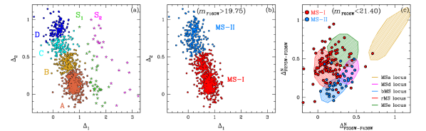
Figure 7: (a) Reproduction of panel (c) of Fig. 4. (b) similar to panel (a), but for MS-I and MS-II stars below the MS knee ($m_{\rm F160W}<19.75$). The brighter ($m_{\rm F606W}>21.4$) stars of MS-I and MS-II are also measured in F275W, F336W and F438W. We applied to these bright stars the same transformations used in Bellini et al. (2017c) to derive the $\Delta^{\rm N}_{\rm F275W-F336W}$ versus $\Delta^{\rm N}_{\rm F336W-F438W}$ chromosome map (panel c, see also their Fig. 10). On this, plane we highlighted the regions (colored shaded areas) occupied by the main population groups of Bellini et al. (2017c): MSa in yellow, MSd in magenta, bMS in azure, rMS in red, MSe in green. The brighter MS-I and MS-II stars are shown as red and blue solid circles, respectively. We find MS-I stars mainly overlapped to the rMS and MSe loci, and MS-II stars to the bMS and MSd loci.

We have defined $\mu_{\rm tan}$ so that it is positive for a counter-clockwise rotation in a righthanded Cartesian system in the plane of the sky. Since $\omega$ Cen is also rotating counter-clockwise, populations with excess rotation have positive $\langle$$\mu_{\rm tan}$$\rangle$, while the opposite is true for populations rotating more slowly. This implies that 1G stars, which are also characterized—on average—by a skewed $\mu_{\rm tan}$ distribution, are rotating faster than 2G stars, which is the main result of this Section. The difference is $0.084\pm 0.017$ ${\rm mas}\,{\rm yr}^{-1}$(i.e., $\sim 2$ ${\rm km}\,{\rm s}^{-1}$). For comparison, the overall mean rotation velocity at the position of field F1 is believed to be $\sim 5$ ${\rm km}\,{\rm s}^{-1}$ (e.g., van de Ven et al. 2006). A direct measurement of the differential rotation of $\omega$ Cen as a function of radius goes beyond the scope of the present work, but will be the subject of a stand-alone paper in this series once all the data of the remaining fields F0, F2, and F3 have been collected.

3.6 A note on white dwarfs

Our PM catalog includes 29 relatively bright WD stars (see, e.g., panel (k) of Fig. 3). Their velocity dispersion, computed over the entire field are as follows: $\sigma_{\mu}=8.39\pm 0.88$ ${\rm km}\,{\rm s}^{-1}$, $\sigma_{\rm rad}=8.98\pm 1.32$ ${\rm km}\,{\rm s}^{-1}$, and $\sigma_{\rm tan}=7.78\pm 1.17$ ${\rm km}\,{\rm s}^{-1}$. The resulting deviation from radial-to-tangential isotropy is $-0.13\pm 0.18$. These values are consistent with those obtained for the mPOPs on the MS of the cluster. We also computed the median WD motion along the $\alpha\cos\delta$, $\delta$, radial and tangential directions. All these values are listed in Table 2. Given the large errors due to small-number statistics, nothing definitive can be said about the level of anisotropy of WDs in our field F1, or if WDs are rotating faster or slower than MS stars. We will briefly return on the kinematics of WDs at the end of Sect. 4.

3.7 Who’s who?

In this section, we want to see if it is possible to connect the six populations identified below the MS knee (Paper I) to the five population groups (or even directly to the 15 distinct populations) analyzed by Bellini et al. (2017c) on the upper MS in the core of the cluster. The meta-groups MS-I and MS-II play a pivotal role: since they extend through the entire MS at our disposal, they share over $\gtrsim 2$ $m_{\rm F606W}$ magnitudes with the six populations of Paper I near the faint end of the MS, and can make use of F275W, F336W and F438W filters in a $\sim 1$ $m_{\rm F606W}$ magnitude bin near the bright limit of our PM catalog, so that we can apply the same selections criteria used by Bellini et al. (2017c) to isolate the five population groups in the cluster’s core.

Panel (a) of Fig. 7 is a replica of panel (c) of Fig. 4, with the six populations of Paper I. On the same plane in panel (b), we color-coded MS-I and MS-II below the MS knee in red and azure, respectively. Clearly, MS-I stars are made up of populations A and B, and MS-II stars are constituted by population C and D stars. Neither the MS-I nor the MS-II overlaps with populations S₁ and S₂, because of the way these stars were selected in Paper I.

We applied to MS-I and MS-II stars in the brightest $\sim 1$ $m_{\rm F606W}$ magnitude bin the same selections criteria of Bellini et al. (2017c) to reproduce the $\Delta^{N}_{\rm F275W-F336W}$ versus $\Delta^{N}_{\rm F336W-F438W}$ chromosome map of their Fig. 10. In panel (c) of Fig. 7 we show this chromosome map for the bright MS-I and MS-II stars in our PM catalog.

The shaded regions highlight the loci of the bulk of the five populations groups identified in Bellini et al. (2017c). On this panel only, the color of the shaded regions refer to the colors adopted by Bellini et al. (2017c) to distinguish the five population groups: MSa in yellow, rMS in red, bMS in azure, MSd in magenta, and MSe in green. MS-I and MS-II stars are shown as red and blue solid circles, respectively. MS-I stars mostly overlap with the bMS and MSd loci, while rMS stars mostly overlap with the rMS and MSe loci.

From the analysis of Bellini et al. (2017c), only $\sim 3.5$% of the bright MS stars in the core of the cluster are MSa stars. In addition, studies of the radial distribution of RGB stars Bellini et al. (2009a) show that the relative number of RGBa stars (the progeny of the MSa) over that of the metal-poor RGB group (the progeny of MS-I stars) halves from the cluster center out to $\sim 17^{\prime}$ where our field F1 lies. There are a total of 137 stars plotted in panel (c) of Fig. 7, and only one MS-I star is within the MSa locus. This star could actually be a MSa star, or it could be an outlier. Either way, population abundances and radial distributions tell us that we should not expect to have more than 1–2 MSa stars in panel (c), which is what we observe.

MS-I stars in panel (c) are mostly on the rMS locus, while in panel (b) they are mostly located where population A stars are. This implies that population A stars belong to the same population group as rMS stars, while population B stars are more likely associated with the MSe.

The identification of MS-II stars is less secure. Population D stars are slightly more abundant than population C stars in panel (a), and MS-I stars in panel (c) are slightly more abundant around the bMS locus rather than around the MSd locus. It is tempting to associate the population C to the MSd group, and the population D to the bMS group.

We are left with populations S₁ and S₂. Statistically speaking, either one can be associated to the MSa. Note, however, that the MSa is the most extreme population group of the cluster in terms of chemical abundance (${\rm[Fe/H]}\simeq-0.7$ (e.g., Norris & Da Costa 1995; Pancino et al. 2002; Johnson et al. 2008, 2009; Marino et al. 2010, 2011), and possibly He abundance up to $Y=0.40$ (Norris 2004; Bellini et al. 2010, 2017c, Paper I). Population S₂ is the most extreme in terms of anisotropy (Fig. 5 and Table 2) and possibly differential rotation (Fig. 6 and Table 3), so it is tempting to associate the kinematically-extreme S₂ stars to the chemically-extreme MSa.

Kinematically, the population S₁ looks more similar to MS-I stars than to MS-II stars, so that S₁ stars should belong to either the rMS or the MSe groups. Bellini et al. (2017c) argued that the four subpopulations that form the MSe group could actually be split into two, with the two least-populated MSe3 and MSe4 subpopulations forming a stand-alone group. MSe3 and MSe4 stars account for just about 3% of MS stars in the core of the cluster, and S₁ stars account for 2.3% of the stars below the MS knee. We tentatively associate S₁ stars to the MSe3 and MSe4 subpopulations.

4 State of energy equipartition

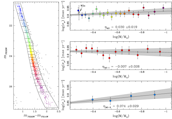
Figure 8: On the left, the $m_{\rm F606W}$ versus $m_{\rm F606W}-m_{\rm F814W}$ CMD of the MS divided into 20 equally-populated bins, colored from blue to purple moving towards fainter stars. We used the same Dotter et al. (2008) isochrones employed in Paper I to transform stellar magnitudes into solar masses, weighting for the contribution of MS-I and MS-II stars in each bin. The top-right panel shows the combined velocity-dispersion profile of these bins as a function of stellar mass in a $\log$-$\log$ plane. For completeness, we also show the location of WDs stars (white diamond) with assumed average mass of 0.52 $\mathrm{M}_{\odot}$. The slope of the straight-line fit to the MS points provides an estimate of the stage of energy equipartition of the cluster in our field. We find $\eta_{\rm MS}\simeq 0.03$. We also computed the state of energy equipartition separately for MS-I (red, middle-right panel) and MS-II (azure, bottom-right panel) stars. See the text for details.

By and large, GCs are assumed to evolve over many two-body relaxation times towards a state of energy equipartition, for which the velocity dispersion scales with stellar mass as $\sigma_{\mu}\propto m^{-\eta}$, with $\eta=0.5$ (e.g., Spitzer 1969, 1987). Recently, Trenti & van der Marel (2013) and Bianchini et al. (2016) have shown that this simple picture is incorrect. In particular, Trenti & van der Marel (2013) used $N$-body simulations to show that GCs reach a maximum value $\eta_{\rm max}\approx 0.15$ in the core, with $\eta$ eventually asymptotically declining to the value $\sim 0.08$. In the cluster outskirts, the energy-equipartition indicator $\eta$ slowly evolves from zero to $\sim 0.08$ (see, e.g., Figs. 6 and 7 of Trenti & van der Marel 2013). The difference between the old and the new pictures can be understood as a consequence of the Spitzer instability for two-component systems, extended by Vishniac (1978) to a continuous mass spectrum.

Concerning $\omega$ Cen, Trenti & van der Marel (2013) analyzed the PM catalog of Anderson & van der Marel (2010) of MS stars in the core of cluster, and found $\eta\approx 0.2$ for stars in the mass range $0.5\leq\mathrm{M}_{\odot}\leq 0.8$. Bellini et al. (2013) extended the mass range in the same field down to $\sim 0.3\,\mathrm{M}_{\odot}$, and found $\eta=0.16\pm 0.05$. These values imply that the core of the cluster is somewhere in between being in no energy equipartition and in full equipartition, and close to the peak value $\eta_{\rm max}$.

To measure the state of energy equipartition in field F1 we proceeded as follows. We divided the MS of the cluster into 20 equally-populated magnitude bins in $m_{\rm F606W}$ (about 90 stars in each bin, left panel of Fig. 8). We color-coded each bin from blue to yellow to purple moving from the brighter to the fainter bin.

To convert magnitudes into stellar masses, we fitted the same two Dotter et al. (2008) isochrones the MS-I and MS-II meta-groups that we had applied in Paper I. MS-I stars are well fitted by an isochrone with ${\rm[Fe/H]}=-1.7$ and primordial Helium abundance (${\rm Y}=0.246$). MS-II stars are modeled with a ${\rm[Fe/H]}=-1.40$, ${\rm Y=0.40}$ isochrone. For each magnitude bin, we computed the median mass of MS-I and MS-II stars within. We noted that 25% of MS stars are MS-II stars, while 75% are MS-I stars (or a MS-I/MS-II ratio of 0.34, in full agreement with the bMS/rMS ratio of $0.34\pm 0.05$ computed by Bellini et al. (2009a) for bright MS stars in the same field). We assigned a weight of 0.75 and of 0.25 to the computed median masses of MS-I and MS-II stars in each bin, and averaged them together.

A direct way to estimate the energy-equipartition indicator $\eta$ is to fit a least-squares straight line to the computed $\sigma_{\mu}$ of the 20 MS bins versus mass in a $\log$-$\log$ plane (top-right panel in Fig. 8). Points are color-coded according to the magnitude bins on the CMD. We obtain $\eta_{\rm MS}=0.030\pm 0.019$. The gray shaded region shows the $\pm 1\sigma$ error in the slope. MS stars in field F1 are consistent with being in nearly no energy equipartition, in agreement with the predictions of Trenti & van der Marel (2013).

Trenti & van der Marel (2013) describe a canonical $N$-body model for the interpretation of equipartition in $\omega$ Cen and other GCs. The value $\eta=0.16\pm 0.05$ observed near the center of $\omega$ Cen is roughly the maximum $\eta$ value attained in this model. At the time when this maximum $\eta$ is attained near the center, the model value of $\eta$ at a projected radius equal to that of field F1 is only $0.012$. This is lower because the relaxation times are much longer in the outskirts of the cluster. The observed value $\eta_{\rm MS}=0.030\pm 0.019$ is consistent with this at the 1$\sigma$ level. This provides an observational validation of the radial dependence of the partial energy equipartition predicted by $N$-body models.

In addition, we also computed the state of energy equipartition separately for MS-I and MS-II stars. To do this, we lowered the number of magnitude bins in order to keep the same number of stars (about 90) in each bin. Because of saturation in the long F606W exposures, our mass ranges are $0.1\lesssim\mathrm{M}_{\odot}\lesssim 0.6$ for the MS-I meta-group, and $0.1\lesssim\mathrm{M}_{\odot}\lesssim 0.5$ for the MS-II meta-group. Results are shown in the middle-right (MS-I) and bottom-right (MS-II) panels of Fig. 8. MS-I stars are consistent with being in no energy equipartition, while there is some marginal evidence that MS-II stars have $\eta_{\rm MS-II}\gtrsim 0$.

As a side note, the velocity dispersion of MS stars we find (about 8 ${\rm km}\,{\rm s}^{-1}$) is consistent with that based on spectra of RGB stars, and reported by van de Ven et al. (2006) at the same cluster distance (about 17^′). Because of the relatively short evolutionary time scales of the sub-giant-branch and the RGB, RGB stars have the same “kinematic” mass of MS turn-off stars (or about $0.8\,\mathrm{M}_{\odot}$). The fact that stars about a factor of two more massive than the typical MS stars studied here ($\sim$0.35 $\mathrm{M}_{\odot}$) have the same velocity dispersion is a further proof that $\omega$ Cen is not in equipartition in our field.

Finally, $\omega$ Cen hosts two distinct WD cooling sequences (Bellini et al. 2013), easily identifiable on UV-based CMDs. The blue WD cooling sequence is populated by the evolved stars of the He-normal (1G) component ($\sim 0.55\,\mathrm{M}_{\odot}$ CO-core DA objects), while the red WD sequence hosts the end products of the He-rich, 2G populations ($\sim 0.46\,\mathrm{M}_{\odot}$ objects, of which $\sim 10$% are CO-core and $\sim 90$% are He-core WDs). A detailed analysis of the WD cooling sequences of the cluster in our four fields F0–F3 will be the subject of a future paper in this series. For now, we can provide insights about the 29 WDs we have identified in field F1 (Sect. 3.6). These WDs are aligned on a single sequence in the $m_{\rm F606W}$ versus $m_{\rm F606W}-m_{\rm F814W}$ CMD (see, e.g., Fig. 3k). If WDs follow the same radial gradient as MS stars, than we expect a 1G/2G ratio of 0.34, which translates into an average per-star WD mass of $\sim 0.52\,\mathrm{M}_{\odot}$. Given a $\sigma_{\mu}=8.39\pm 0.88$ ${\rm km}\,{\rm s}^{-1}$, WD stars are found to follow the same trend of MS stars (white diamond in the top-right panel in Fig. 8), well within their measured errors. Given the large error bars, even a large over- or under-estimate of their mass would still put them on the fitted line. This suggests that also WDs in the field are consistent with not being in energy equipartition.

5 Conclusions

As part of the “HST large programme of $\omega$ Centauri” (GO-14118 + GO-14662, PI: Bedin, L. R.), we have computed high-precision PMs of MS stars of the GC $\omega$ Cen down to near the HBL in one of the four fields imaged by the program. This field, located at about 3.5 half-light radii from the cluster center, is the first for which all observations have now been completed. Well-measured stars in the field have a typical PM error of $\sim 10\,\mu$as yr^-1.

We used the same population selections defined in Paper I to study the internal kinematics of the MS-I (1G) and MS-II (2G) meta-groups, as well as of the six populations identified below the MS knee using a combination of optical and IR filters. We find no significant trends of the velocity dispersion as a function of distance from the cluster center within our field. All populations have similar velocity dispersions along the radial (i.e., towards the cluster’s center) component of the motion, $\mu_{\rm rad}$. The velocity dispersions along the tangential component of the motion, $\mu_{\rm tan}$, are instead significantly different between MS-I and MS-II stars, and between the six populations below the MS knee. These kinematic differences result in 1G stars (MS-I, populations A, B, and S₁) being isotropic or nearly isotropic, while 2G stars (MS-II, populations C, D and, S₂) are radially anisotropic. These results are consistent with what was found at large radial distances in two other massive GCs: 47 Tuc (Richer et al. 2013) and NGC 2808 (Bellini et al. 2015a), and can be interpreted as 2G stars slowly diffusing towards the cluster’s outer regions preferentially on radial orbits.

The $\mu_{\rm tan}$ distribution of $\omega$ Cen stars is found to be slightly skewed towards negative $\mu_{\rm tan}$ values. Recently, Heyl et al. (2017) also measured some degree of skewness in the $\mu_{\rm tan}$ distribution of 47 Tuc stars, and pointed towards differential rotation being the cause of the observed skewness. We found 1G stars to be slightly but significantly skewed, while 2G stars have a more symmetric $\mu_{\rm tan}$ distribution. In addition, the median values $\langle$$\mu_{\rm tan}$$\rangle$ of each population indicate that 1G stars must have a higher velocity rotation in the plane of the sky than 2G stars.

We identified MS-I and MS-II over the entire $m_{\rm F606W}$ magnitude range in our PM catalog, so that these population meta-groups share over two magnitudes in common with the six populations below the MS knee. On the bright end of the MS, we used the photometric information of the shallower F275W, F336W, and F438W photometry and applied to them the same selection criteria used by Bellini et al. (2017c) to identify 15 distinct populations (organized into 5 main groups) in the core of the cluster. Using MS-I and MS-II stars as a common benchmark, we were able to link the six populations of Paper I to the 5 groups of Bellini et al. (2017c). We find: population A $\Longleftrightarrow$ rMS, B $\Longleftrightarrow$ MSe, C $\Longleftrightarrow$ MSd, D $\Longleftrightarrow$ bMS. The connection of populations S₁ and S₂ to their brighter counterparts is less obvious. Using chemical abundance and kinematic arguments, we tentatively associated population S₁ to the MSe3 and MSe4 populations, and S₂ to the MSa.

We estimated the degree of energy equipartition of MS stars in the mass range $0.1\lesssim\mathrm{M}_{\odot}\lesssim 0.6$. We find $\eta_{\rm MS}=0.030\pm 0.019$. This value is consistent with the $N$-body simulations of Trenti & van der Marel (2013), in which GCs reach at most only partial equipartition. We also estimated the level of energy equipartition separately for 1G (MS-I) and 2G (MS-II) stars. We found the former to have $\eta_{\rm MS-I}=-0.007\pm 0.026$ (no equipartition), and for the latter a value $\eta_{\rm MS-II}=0.074\pm 0.029$, only marginally greater than zero.

We make our astro-photometric catalog publicly available to the astronomical community through the ApJ website. A description of the catalog is given in Sect A.

Appendix A Description of the astro-photometric catalogs

The catalog presented here is divided into an astrometric file containing stellar positions and PMs, and one file per filter with the photometric information. These files contain the same number of ordered entries (one line per star) so that, e.g., the PM data of line 100 in the astrometric file and the photometry of line 100 of any of the photometric files refer to the same star.

Table 4 shows the first 10 lines of the photometric file relative to the F814W filter. The $o$ parameter tells us the initial (i.e., before neighbor subtraction) ratio between the light within the fitting radius due to nearby neighbors and the light of the star. The quantities n_f and n_u record in how many single exposures a star was found, and how many single measurements were used to compute photometric quantities, respectively. The local sky value around each star and its RMS are given in units of e^- at the reference exposure time. To revert VEGA mag values back into instrumental magnitudes $m$ (at the same reference exposure time), the user can simply subtract the adopted calibration zero points, which are given in Table 5. Instrumental magnitudes can then be transformed into fluxes $F$ in unit of electrons: $F=10^{-0.4\times m}$ at the reference exposure time. This way, the user can apply selections based on sigmas over the sky background. A flag value of 99.99 is used for the magnitude RMS when photometry is based on only one measurement. A flag value of zero is used for all the other quantities when a star is not measured in a particular filter. Undertermined local sky values are flagged with a value of 0.0, together with the associated sky RMS.

An extract of the astrometric file is given in Table 6. The X and Y positions refer to our right-handed Cartesian master frame, which has a pixel scale of 40 mas pixel^-1. The values $\chi^{2}_{\rm X}$ and $\chi^{2}_{\rm Y}$ are intended as reduced $\chi^{2}$ values. The temporal baseline used to compute PMs is indicated as $\Delta$time. The ID entries in the last column of the Table are the internal IDs of the reduction process.

Table 4: First ten lines of the photometric catalog for filter F814W.

VEGA mag	RMS mag	QFIT	$o$	RADXS	nf	nu	local sky (e-)	RMS sky (e-)
25.7403	99.9900	0.8760	2.00481	$-$0.0945	1	1	0.0	0.0
25.0999	0.0308	0.9530	0.53509	$-$0.0169	2	2	0.0	0.0
21.8048	0.0003	1.0000	0.00000	$-$0.0026	2	2	82.5	51.4
20.8638	0.0099	0.9950	0.00000	$-$0.0052	2	2	212.6	115.0
25.7705	0.0335	0.8170	0.02167	0.1728	2	2	14.0	9.1
23.2805	0.0070	0.9970	0.00000	0.0046	2	2	23.5	14.1
19.7016	0.0011	1.0000	0.00000	$-$0.0008	2	2	582.2	318.3
22.0618	0.0015	0.9990	0.00000	$-$0.0052	2	2	72.6	38.5
21.0557	0.0431	0.9820	0.00000	0.0156	2	2	154.8	89.0
24.8920	0.0153	0.8930	0.00000	0.0910	2	2	0.0	0.0
$[\dots]$	$[\dots]$	$[\dots]$	$[\dots]$	$[\dots]$	$[\dots]$	$[\dots]$	$[\dots]$	$[\dots]$

Table 5: Adopted VEGA-mag photometric zero points.

WFC3 Filter	VEGA zero point
F606W	33.5960
F814W	32.2910
F110W	26.1749
F160W	24.7457

Table 6: First ten lines of the astrometric catalog of field F1.

R.A.	Decl.	X	Y	$\!\!\!\Delta\mu_{\alpha}^{\rm r}\cos\delta$	$\sigma_{\mu_{\alpha}^{\rm r}\cos\delta}$	$\!\!\!\Delta\mu_{\delta}^{\rm r}$	$\sigma_{\mu_{\delta}^{\rm r}}$	$\chi^{2}_{\rm X}$	$\chi^{2}_{\rm Y}$	nf	nu	$\!\!\!\Delta$time	$\!\!\!\Delta\mu^{\rm c}_{\alpha}\cos\delta$	$\sigma_{\mu^{\rm c}_{\alpha}\cos\delta}$	$\!\!\!\Delta\mu^{\rm c}_{\delta}$	$\sigma_{\mu^{\rm c}_{\delta}}$	ID
deg	deg	pixel	pixel	${\rm mas}\,{\rm yr}^{-1}$	${\rm mas}\,{\rm yr}^{-1}$	${\rm mas}\,{\rm yr}^{-1}$	${\rm mas}\,{\rm yr}^{-1}$					yr	${\rm mas}\,{\rm yr}^{-1}$	${\rm mas}\,{\rm yr}^{-1}$	${\rm mas}\,{\rm yr}^{-1}$	${\rm mas}\,{\rm yr}^{-1}$
(1)	(2)	(3)	(4)	(5)	(6)	(7)	(8)	(9)	(10)	(11)	(12)	(13)	(14)	(15)	(16)	(17)	(18)
201.43076135593	$-$47.69362075406	2384.4761	1573.5081	0.07308	0.22500	$-$0.57616	0.14524	2.7706	1.1542	17	14	15.12775	0.04832	0.22749	$-$0.66180	0.14989	48
201.43075950173	$-$47.69362012573	2384.5884	1573.5647	$-$0.56564	0.19632	$-$0.24208	0.17492	3.1617	2.5091	17	15	15.12775	$-$0.59040	0.19916	$-$0.32772	0.17881	49
201.38848444873	$-$47.69361315403	4945.5029	1574.6746	0.08380	0.01828	0.31376	0.01812	0.6405	0.6287	21	21	15.12775	0.05456	0.03819	0.34896	0.04023	53
201.41179992503	$-$47.69395514603	3533.1177	1543.8008	$-$0.49612	0.01724	4.82204	0.01676	0.6072	0.5738	19	19	15.12725	$-$0.47240	0.03873	4.86792	0.03304	60
201.38992925597	$-$47.69366611367	4857.9800	1569.9146	4.54220	0.44612	6.40428	0.32588	11.0648	5.9048	18	18	15.12775	4.54856	0.44737	6.42320	0.32772	66
201.38889075924	$-$47.69363046474	4920.8897	1573.1185	$-$4.67476	0.04188	6.80408	0.03684	0.6947	0.5374	17	15	15.12764	$-$4.69240	0.05391	6.83928	0.05124	67
201.41577053661	$-$47.69392905370	3292.5891	1546.0909	$-$0.52392	0.20692	0.01040	0.19460	1.0987	0.9716	8	8	2.00041	$-$0.52296	0.21015	0.08496	0.19766	68
201.41597236104	$-$47.69371429518	3280.3579	1565.4168	0.20084	0.01504	$-$0.02724	0.01548	0.3271	0.3463	19	17	15.12775	0.17764	0.03818	0.01004	0.03636	72
201.41529419354	$-$47.69363345110	3321.4375	1572.7040	3.83644	0.01900	6.18012	0.02324	0.8338	1.2490	24	23	15.13011	3.79600	0.03939	6.20736	0.04021	74
201.40595793882	$-$47.69364086614	3887.0039	1572.1504	3.32892	0.20576	7.00512	0.29964	5.6617	12.0045	16	15	15.12775	3.36304	0.20901	7.04240	0.30114	81
$[\dots]$	$[\dots]$	$[\dots]$	$[\dots]$	$[\dots]$	$[\dots]$	$[\dots]$	$[\dots]$	$[\dots]$	$[\dots]$	$[\dots]$	$[\dots]$	$[\dots]$	$[\dots]$	$[\dots]$	$[\dots]$	$[\dots]$	$[\dots]$
Note. The superscripts “r” and “c” of columns (5), (6), (7), (8), and (14), (15), (16), (17), respectively, refer to raw (r) and corrected (c) PMs, as described in Sects. 2.5 and 2.6.

References

- Anderson (1997) Anderson, J., Ph.D. thesis, Univ. of California, Berkeley, 1997
- Anderson & King (2006) Anderson, J., & King, I. R. 2006, ACS/ISR 2006-01 (Baltimore, MD: STScI), available online at http://www.stsci.edu/hst/acs/documents/isrs
- Anderson et al. (2006) Anderson, J., Bedin, L. R., Piotto, G., Yadav, R. S., & Bellini, A. 2006, A&A, 454, 1029
- Anderson et al. (2008) Anderson, J., Sarajedini, A., Bedin, L. R., et al. 2008, AJ, 135, 2055
- Anderson & Bedin (2010) Anderson, J., & Bedin, L. R. 2010, PASP, 122, 1035
- Anderson & van der Marel (2010) Anderson, J., & van der Marel, R. P. 2010, ApJ, 710, 1032
- Bastian et al. (2013) Bastian N. et al. 2013, MNRAS, 436, 2398
- Bedin et al. (2004) Bedin, L. R., Piotto, G., Anderson, J., et al. 2004, ApJ, 605, L125
- Bedin et al. (2008) Bedin, L. R., King, I. R., Anderson, J., et al. 2008, ApJ, 678, 1279-1291
- Bellini & Bedin (2009) Bellini, A., & Bedin, L. R. 2009, PASP, 121, 1419
- Bellini et al. (2009a) Bellini, A., Piotto, G., Bedin, L. R., et al. 2009, A&A, 507, 1393
- Bellini et al. (2009b) Bellini, A., Piotto, G., Bedin, L. R., et al. 2009, A&A, 493, 959
- Bellini et al. (2010) Bellini, A., Bedin, L. R., Piotto, G., et al. 2010, AJ, 140, 631
- Bellini et al. (2011) Bellini, A., Anderson, J., & Bedin, L. R. 2011, PASP, 123, 622
- Bellini et al. (2013) Bellini, A., Anderson, J., Salaris, M., et al. 2013, ApJ, 769, L32
- Bellini et al. (2013) Bellini, A., van der Marel, R. P., & Anderson, J. 2013, Mem. Soc. Astron. Italiana, 84, 140
- Bellini et al. (2014) Bellini, A., Anderson, J., van der Marel, R. P., et al. 2014, ApJ, 797, 115
- Bellini et al. (2015a) Bellini, A., Vesperini, E., Piotto, G., et al. 2015, ApJ, 810, L13
- Bellini et al. (2015b) Bellini, A., Renzini, A., Anderson, J., et al. 2015, ApJ, 805, 178
- Bellini et al. (2017a) Bellini, A., Anderson, J., Bedin, L. R., et al. 2017, ApJ, 842, 6
- Bellini et al. (2017b) Bellini, A., Anderson, J., van der Marel, R. P., et al. 2017, ApJ, 842, 7
- Bellini et al. (2017c) Bellini, A., Milone, A. P., Anderson, J., et al. 2017, ApJ, 844, 164
- Bellini et al. (2017d) Bellini, A., Bianchini, P., Varri, A. L., et al. 2017, ApJ, 844, 167
- Bender et al. (1994) Bender, R., Saglia, R. P., & Gerhard, O. E. 1994, MNRAS, 269, 785
- Bianchini et al. (2016) Bianchini, P., van de Ven, G., Norris, M. A., Schinnerer, E., & Varri, A. L. 2016, MNRAS, 458, 3644
- Bohlin (2016) Bohlin, R. C. 2016, AJ, 152, 60
- Boyles et al. (2011) Boyles, J., Lorimer, D. R., Turk, P. J., et al. 2011, ApJ, 742, 51
- Bulmer (1979) Bulmer, M. G., 1979, “Principles of Statistics”. Dover.
- Cramer (1997) Cramer, D., 1997, “Basic Statistics for Social Research”. Routledge.
- D’Ercole et al. (2008) D’Ercole A., Vesperini E., D’Antona F., McMillan, S.L.W., Recchi, S., 2008, MNRAS, 391, 825
- D’Souza & Rix (2013) D’Souza, R., & Rix, H.-W. 2013, MNRAS, 429, 1887
- Decressin et al. (2007) Decressin, T., Meynet, G., Charbonnel C. Prantzos, N.,Ekstrom,S. 2007, å, 464, 1029
- Di Nino et al. (2008) Di Nino, D., Makidon, R. B., Latto, M., et al. 2008, ACS-ISR 2008-03 (Baltimore, MD: STScI), available online at http://www.stsci.edu/hst/acs/documents/isrs/
- Dickens & Woolley (1967) Dickens, R. J., & Woolley, R. v. d. R. 1967, Royal Greenwich Observatory Bulletins, 128, 255
- Dotter et al. (2008) Dotter, A., Chaboyer, B., Jevremović, D., et al. 2008, ApJS, 178, 89-101
- Ferraro et al. (2002) Ferraro, F. R., Bellazzini, M., & Pancino, E. 2002, ApJ, 573, L95
- Gaia Collaboration et al. (2016a) Gaia Collaboration, Brown, A. G. A., Vallenari, A., et al. 2016, A&A, 595, A2
- Gaia Collaboration et al. (2016b) Gaia Collaboration, Prusti, T., de Bruijne, J. H. J., et al. 2016, A&A, 595, A1
- Heyl et al. (2017) Heyl, J., Caiazzo, I., Richer, H., et al. 2017, ApJ, 850, 186
- Harris (1996) Harris, W. E. 1996, AJ, 112, 1487, 2010 edition
- Johnson et al. (2008) Johnson, C. I., Pilachowski, C. A., Simmerer, J., & Schwenk, D. 2008, ApJ, 681, 1505-1523
- Johnson et al. (2009) Johnson, C. I., Pilachowski, C. A., Michael Rich, R., & Fulbright, J. P. 2009, ApJ, 698, 2048
- King et al. (2012) King, I. R., Bedin, L. R., Cassisi, S., et al. 2012, AJ, 144, 5
- Lee et al. (1999) Lee, Y.-W., Joo, J.-M., Sohn, Y.-J., et al. 1999, Nature, 402, 55
- Libralato et al. (2018) Libralato, M., Bellini, A., Bedin, L. R., et al. 2018, arXiv:1801.01502 (Paper III)
- Marino et al. (2010) Marino, A. F., Piotto, G., Gratton, R., et al. 2010, Light Elements in the Universe, 268, 183
- Marino et al. (2011) Marino, A. F., Milone, A. P., Piotto, G., et al. 2011, ApJ, 731, 64
- Meylan & Mayor (1986) Meylan, G., & Mayor, M. 1986, A&A, 166, 122
- Milone et al. (2017a) Milone, A. P., Piotto, G., Renzini, A., et al. 2017, MNRAS, 464, 3636
- Milone et al. (2017b) Milone, A. P., Marino, A. F., Bedin, L. R., et al. 2017, MNRAS, 469, 800 (Paper I)
- Norris & Da Costa (1995) Norris, J. E., & Da Costa, G. S. 1995, ApJ, 447, 680
- Norris (2004) Norris, J. E. 2004, ApJ, 612, L25
- Pancino et al. (2000) Pancino, E., Ferraro, F. R., Bellazzini, M., Piotto, G., & Zoccali, M. 2000, ApJ, 534, L83
- Pancino et al. (2002) Pancino, E., Pasquini, L., Hill, V., Ferraro, F. R., & Bellazzini, M. 2002, ApJ, 568, L101
- Pancino et al. (2017) Pancino, E., Bellazzini, M., Giuffrida, G., & Marinoni, S. 2017, MNRAS, 467, 412
- Piotto et al. (2015) Piotto, G., Milone, A. P., Bedin, L. R., et al. 2015, AJ, 149, 91
- Platais et al. (2003) Platais, I., Wyse, R. F. G., Hebb, L., Lee, Y.-W., & Rey, S.-C. 2003, ApJ, 591, L127
- Renzini et al. (2015) Renzini, A., D’Antona, F., Cassisi, S., et al. 2015, MNRAS, 454, 4197
- Richer et al. (2013) Richer, H. B., Heyl, J., Anderson, J., et al. 2013, ApJ, 771, L15
- Sollima et al. (2007) Sollima, A., Ferraro, F. R., Bellazzini, M., et al. 2007, ApJ, 654, 915
- Spitzer (1969) Spitzer, L., Jr. 1969, ApJ, 158, L139
- Spitzer (1987) Spitzer, L. 1987, Princeton, NJ, Princeton University Press, 1987, 191 p.,