Solar Flares and the Axion Quark Nugget Dark Matter Model

Abstract

We advocate the idea that the nanoflares conjectured by Parker long ago to resolve the corona heating problem, may also trigger the larger solar flares. The arguments are based on the model where emission of extreme ultra violet (EUV) radiation and soft x-rays from the Sun are powered externally by incident dark matter particles within the Axion Quark Nugget (AQN) Dark Matter Model. The corresponding annihilation events of the AQNs with the solar material are identified with nanoflares. This model was originally invented as a natural explanation of the observed ratio $\Omega_{\rm dark}\sim\Omega_{\rm visible}$ when the DM and visible matter densities assume the same order of magnitude values. This model gives a very reasonable intensity of EUV radiation without adjustments of any parameters in the model. When the same nuggets enter the regions with high magnetic field they serve as the triggers igniting the magnetic reconnections which eventually may lead to much larger flares.

Technically, the magnetic reconnection is ignited due to the shock wave which inevitably develops when the dark matter nuggets enter the solar atmosphere with velocity $v_{\rm AQN}\sim~{}600~{}{\rm km/s}$ which is much higher than the speed of sound $c_{s}$, such that the Mach number $M=v_{\rm AQN}/c_{s}\gg 1$. These shock waves generate very strong and very short impulses expressed in terms of pressure $\Delta p/p\sim M^{2}$ and temperature $\Delta T/T\sim M^{2}$ in vicinity of (would be) magnetic reconnection area. We find that this mechanism is consistent with x -ray observations as well as with observed jet like morphology of the initial stage of the flares. The mechanism is also consistent with the observed scaling of the flare distribution $dN\sim W^{-\alpha}dW$ as a function of the flare’s energy $W$. We also speculate that the same nuggets may trigger the sunquakes which are known to be correlated with large flares.

1 Introduction

A variety of anomalous solar phenomena still defy conventional theoretical understanding. For example, the detailed physical processes that heat the outer atmosphere of the Sun to $10^{6}$K remain a major open issue in astrophysics, see e.g. [1] for review and references on the original results. This persisting puzzle is characterized by the following observed anomalous behaviour of the sun: the quiet Sun emits an extreme ultra violet (EUV) radiation with a photon energy of order of hundreds of eV which cannot be explained in terms of any conventional astrophysical phenomena; the total energy output of the corona is quite small, see (1) below. However, it never drops to zero as time evolves. To be more specific, the total intensity of the observed EUV and soft x-ray radiation (averaged over time) can be estimated as follows,

$$L_{\odot~{}(\rm from~{}Corona)}\sim 10^{30}\cdot\frac{\rm GeV}{\rm s}\sim 10^{27}\cdot\frac{\rm erg}{\rm s}.$$ (1)

which represents about $(10^{-7}-10^{-6})$ fraction of the solar luminosity.

At the transition region, the (quiet Sun) temperature continues to rise very steeply until it reaches a few $10^{6}$ K, i.e., being a few 100 times hotter above the underlying photosphere, and this within an atmospheric layer thickness of only 100 km or even much less. Therefore, after several decades of research, it may be that the answer on these (and many others related) questions lies in a new physics.

Figure 1: The “multiplication spectrum” is defined as $Y(J)\equiv\Theta_{1}(J)\cdot\Theta_{2}(J)\cdot\Theta_{3}(J)\cdot\Theta_{4}(J)$, where $\Theta$ is the deflection angle related to the gravitational lensing analysis. The subscript (1-4) denotes the four solar cycles (1975-1986, 1986-1997, 1997-2009, 2009-2014) and $J$ denotes the bin number with widths ($6^{\circ},12^{\circ},16^{\circ}$). The plots are taken from [2].

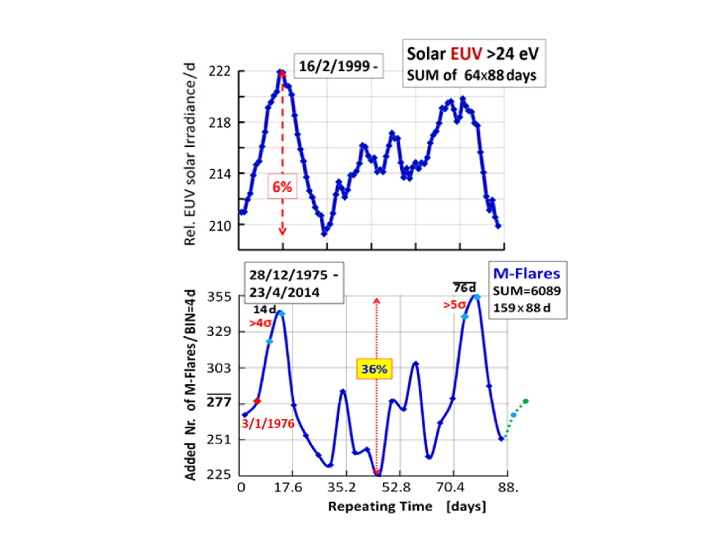
Figure 2: This plot demonstrates the connection between the relative EUV radiation (top) and the number of M-flares during the same period of time (bottom). The BIN size is 1 day for the EUV data and 4 days for M-flares analysis. The plots are taken from [2].

It was precisely the main subject of ref.[2] where it was advocated that a number of highly unusual phenomena (including, but not limited to the EUV radiation) observed in solar atmosphere might be related to the gravitational lensing of “invisible” streaming matter towards the Sun. The main argument of ref.[2] is based on analysis of a number of different correlations between the relative orientations of the Sun and its planets on the one hand and the frequency of the observed flares on the other hand of the analysis. As an example of the observed correlations we reproduce on Fig.1 some sample plots for the so-called “multiplication spectrum” from ref. [2] where the frequency of occurring of the X-flares is shown as a function of the Mercury (on the top) and the Earth (on the bottom) heliocentric longitude. We refer to the original paper [2] for the specific discussions, definitions and the details on the data analysis. In this Introduction the only comment we would like to make is that one should not expect any correlations between the X flare occurrences and the position of the planets. Nevertheless, Fig.1 obviously demonstrates that this naive expectation is not quite correct, and that the enhancement is happening around the same heliocentric longitude for Mercury and Earth in spite of the fact that periods of the Earth and Mercury are very different ($T_{\rm Mercury}=87.969$ days) and they appear at this specific heliocentric longitude when the enhancement occurs, in general, at different moments.

One should comment here that “the solar corona heating problem” includes a number of elements which are hard to explain using a conventional framework. In particular, the hot corona cannot be in equilibrium with the $\sim 300$ times cooler solar surface (violating thus the second law of thermodynamics [3]). In order to maintain the quiet Sun high temperature corona, some non-thermally supplied energy must be dissipated in the upper atmosphere [4]. There are many other problems which are nicely stated in review article [5] as follows “everything above the photosphere…would not be there at all”. In particular, the observed x-rays in 1-10 keV energy range in the non-flaring Sun are hard to explain using traditional solar physics [6].

It has been recently argued in [7] that the dark matter AQNs might be the source of the heating of outer atmosphere of the Sun and, therefore, might be directly responsible for the observed EUV radiation and heating the corona. Recently, this proposal has received a strong numerical support [8]. We review the basic arguments supporting this proposal in Section 3. The only comment we would like to make here is that this proposal simultaneously resolves the two problems mentioned above: “solar corona heating” problem and mysterious and unexpected correlation of the solar activity with position of its planets.

To recapitulate: this proposal links the EUV radiation and occurrences of the X, M flares as these two apparently distinct phenomena in fact intimately related as they obviously accompany each other according to Fig.2, and they both are correlated with positions of the planets as argued in [2].

It turns out that if one estimates the extra energy being produced within the AQN dark matter scenario one obtains the total extra energy $\sim 10^{27}{\rm erg}/{\rm s}$ which precisely reproduces (1) for the observed EUV and soft x-ray intensities [7]. The numerical Monte Carlo simulations [8] fully support the estimate (1). Furthermore, the numerical analysis [8] also shows that the energy injection occurs precisely in the vicinity of the transition region at the altitude $\sim 2000$ km. This confirms the order of magnitude estimate [7] that the emission will be mostly in form of the EUV and soft x-rays.

One should emphasize that the production of extra energy is expressed exclusively in terms of known dark matter density $\rho_{\rm DM}\sim 0.3~{}{\rm GeVcm^{-3}}$ and dark matter velocity $v_{\rm DM}\sim 10^{-3}c$ surrounding the Sun without adjusting any parameters of the AQN model, see section 3 below with relevant comments. We interpreted this “numerical coincidence” as an additional argument supporting our proposal that the heating of the corona and the chromosphere is originated form the AQNs entering the solar atmosphere from outer space.

The main purpose of the present work is to present a very specific mechanism which may provide a hint on how these two naively distinct phenomena nevertheless might be closely related to each other. This deep relation between these two distinct effects may shed some light on the nature of the dark matter which (within the AQN paradigm) is the source for both phenomena, the EUV radiation and the flare’s activity. Therefore, increase of the DM flux should lead to some increase of the EUV radiation along with the higher frequency of the flare’s occurrences when averaged over long period of time.

One should emphasize that the AQN dark matter model was originally proposed long ago [9] without any connection to the solar system and the EUV. Rather, the main motivation to develop the AQN dark matter model was to explain in a very natural way the observed similarity between the visible and dark matter densities in the present Universe, i.e. $\Omega_{\rm dark}\sim\Omega_{\rm visible}$.

The paper is organized as follows. In next section 2 we overview the AQN model by paying special attention to the astrophysical and cosmological consequences of this specific dark matter model. In section 3 we highlight the basic arguments of refs. [7, 8] advocating the idea that the annihilation events of the antinuggets with the solar material can be interpreted as the nanoflares conjectured by Parker long ago. In the section 4 we argue that the same AQNs entering the region with the large magnetic field may spark the magnetic reconnection leading to very large flares. In other words, we want to argue that the AQNs may play the role of the triggers initiating the large scale flares in the regions with large magnetic field. To be more specific, we want to argue that the shock waves (which will be always generated as a result of high velocity of the dark matter nuggets entering the solar atmosphere with typical average $v_{\rm AQN}\sim 600{\rm km/s}$ which is much greater than the speed of sound $c_{s}$) can easily initiate the large flares as a result of the magnetic reconnection. In section 5 we review some observations, including x-ray data supporting the basic framework. We also speculate that the sunquakes might be also related to the same AQNs initially entering from outer space and capable to reach the photospheric layer.

2 Axion Quark Nugget (AQN) dark matter model

The AQN model in the title of this section stands for the axion quark nugget model, see original work [9] and short overview [10] with large number of references on the original results reflecting different aspects of the AQN model. In comparison with many other similar proposals it has two unique features:
1. There is an additional stabilization factor in the AQN model provided by the axion domain walls which are copiously produced during the QCD transition in early Universe;
2. The AQNs could be made of matter as well as antimatter in this framework as a result of separation of the baryon charges.

The most important astrophysical implication of these new aspects relevant for the present studies (focusing on different types of flares and sources of the EUV and x-ray radiation in the solar chromosphere and corona) is that quark nuggets made of antimatter store a huge amount of energy which can be released when the anti-nuggets hit the Sun from outer space and get annihilated. This feature of the AQN model is unique and is not shared by any other dark matter models because the dark matter in AQN model is made of the same quarks and antiquarks of the standard model (SM) of particle physics. One should also remark here that the annihilation events of the anti-nuggets with visible matter may produce a number of other observable effects in different circumstances such as rare events of annihilation of anti-nuggets with visible matter in the centre of galaxy, or in the Earth atmosphere, see some references on the original computations in [10] and few comments at the end of this section.

The basic idea of the AQN proposal can be explained as follows: It is commonly assumed that the Universe began in a symmetric state with zero global baryonic charge and later (through some baryon number violating process, the so-called baryogenesis) evolved into a state with a net positive baryon number. As an alternative to this scenario we advocate a model in which “baryogenesis” is actually a charge separation process when the global baryon number of the Universe remains zero. In this model the unobserved antibaryons come to comprise the dark matter in the form of dense nuggets of quarks and antiquarks in colour superconducting (CS) phase. The formation of the nuggets made of matter and antimatter occurs through the dynamics of shrinking axion domain walls, see original papers [11, 12] with many technical details.

The nuggets, after they formed, can be viewed as the strongly interacting and macroscopically large objects with a typical nuclear density and with a typical size $R\sim(10^{-5}-10^{-4})$cm determined by the axion mass $m_{a}$ as these two parameters are linked, $R\sim m_{a}^{-1}$. This relation between the size of nugget $R$ and the axion mass $m_{a}$ is a result of the equilibration between the axion domain wall pressure and the Fermi pressure of the dense quark matter in CS phase. One can easily estimate a typical baryon charge $B$ of such macroscopically large objects as the typical density of matter in CS phase is only few times the nuclear density. However, it is important to emphasize that there are strong constraints on the allowed window for the axion mass, which can be represented as follows $10^{-6}{\rm eV}\leq m_{a}\leq 10^{-2}{\rm eV}$, see original papers [13, 14, 15] and reviews [16, 17, 18, 19, 20, 21, 22, 23] on the theory of the axion and recent progress on axion search experiments.

This axion window corresponds to the range of the nugget’s baryon charge $B$ which largely overlaps with all presently available and independent constraints on such kind of dark matter masses and baryon charges

$$10^{23}\leq|B|\leq 10^{28},$$ (2)

see e.g. [24, 10] for review. The corresponding mass $\cal{M}$ of the nuggets can be estimated as ${\cal{M}}\sim m_{p}B$, where $m_{p}$ is the proton mass, though more precise estimates relating the axion mass $m_{a}$, the baryon nuggets charge $B$ and the nugget’s mass $\cal{M}$ are also available [25].

This model is perfectly consistent with all known astrophysical, cosmological, satellite and ground based constraints within the parametrical range for the mass $\cal{M}$ and the baryon charge $B$ mentioned above (2). It is also consistent with known constraints from the axion search experiments. Furthermore, there is a number of frequency bands where some excess of emission was observed, but not explained by conventional astrophysical sources. Our comment here is that this model may explain some portion, or even entire excess of the observed radiation in these frequency bands, see short review [10] and additional references at the end of this section.

Another key element of this model is the coherent axion field $\theta$ which is assumed to be non-zero during the QCD transition in early Universe. As a result of these $\cal CP$ violating processes the number of nuggets and anti-nuggets being formed would be different. This difference is always of order of one effect [11, 12] irrespectively to the parameters of the theory, the axion mass $m_{a}$ or the initial misalignment angle $\theta_{0}$. As a result of this disparity between nuggets and anti nuggets a similar disparity would also emerge between visible quarks and antiquarks. This is precisely the reason why the resulting visible and dark matter densities must be the same order of magnitude [11, 12]

$$\Omega_{\rm dark}\sim\Omega_{\rm visible}$$ (3)

as they are both proportional to the same fundamental $\Lambda_{\rm QCD}$ scale, and they both are originated at the same QCD epoch. If these processes are not fundamentally related the two components $\Omega_{\rm dark}$ and $\Omega_{\rm visible}$ could easily exist at vastly different scales.

Unlike conventional dark matter candidates, such as WIMPs (Weakly interacting Massive Particles) the dark-matter/antimatter nuggets are strongly interacting and macroscopically large objects, as we already mentioned. However, they do not contradict any of the many known observational constraints on dark matter or antimatter in the Universe due to the following main reasons [26]: They carry very large baryon charge $|B|\gtrsim 10^{23}$, and so their number density is very small $\sim B^{-1}$. As a result of this unique feature, their interaction with visible matter is highly inefficient, and therefore, the nuggets are perfectly qualify as DM candidates. Furthermore, the quark nuggets have very large binding energy due to the large gap $\Delta\sim 100$ MeV in CS phases. Therefore, the baryon charge is so strongly bounded in the core of the nugget that it is not available to participate in big bang nucleosynthesis (bbn) at $T\approx 1$ MeV, long after the nuggets had been formed.

It should be noted that the galactic spectrum contains several excesses of diffuse emission the origin of which is unknown, the best known example being the strong galactic 511 keV line. If the nuggets have the average baryon number in the $\langle B\rangle\sim 10^{25}$ range they could offer a potential explanation for several of these diffuse components. It is important to emphasize that a comparison between emissions with drastically different frequencies in such computations is possible because the rate of annihilation events (between visible matter and antimatter DM nuggets) is proportional to one and the same product of the local visible and DM distributions at the annihilation site. The observed fluxes for different emissions thus depend through one and the same line-of-sight integral

$$\Phi\sim R^{2}\int d\Omega dl[n_{\rm visible}(l)\cdot n_{DM}(l)],$$ (4)

where $R\sim B^{1/3}$ is a typical size of the nugget which determines the effective cross section of interaction between DM and visible matter. As $n_{DM}\sim B^{-1}$ the effective interaction is strongly suppressed $\sim B^{-1/3}$. The parameter $\langle B\rangle\sim 10^{25}$ was fixed in this proposal by assuming that this mechanism saturates the observed 511 keV line [27, 28], which resulted from annihilation of the electrons from visible matter and positrons from anti-nuggets. Other emissions from different frequency bands are expressed in terms of the same integral (4), and therefore, the relative intensities are unambiguously and completely determined by internal structure of the nuggets which is described by conventional nuclear physics and basic QED, see short overview [10] with references on specific computations of diffuse galactic radiation in different frequency bands.

Finally we want to mention that the recent EDGES observation of a stronger than anticipated 21 cm absorption [29] can find an explanation within the AQN framework as recently advocated in [30]. The basic idea is that the extra thermal emission from AQN dark matter at early times produces the required intensity (without adjusting of any parameters) to explain the recent EDGES observation.

3 The AQN annihilation events as nanoflares

We start our overview of the basic results of ref [7] with subsection 3.1 where we present simple estimates of the energetic budget suggesting that the heating of the chromosphere and corona might be due to the annihilation events of the AQN with the solar material. As the next step, in subsection 3.2 we highlight the arguments of ref. [7] suggesting that the corresponding annihilation events heating the corona can be identified with the nanoflares conjectured by Parker long ago [31]. Finally, in subsection 3.3 we describe some recent observations of microflares and flares (along with nanoflares) suggesting that all these phenomena might be in fact tightly connected and originated from the same AQNs in spite of the fact that these phenomena are characterized by drastically different energy scales: from $10^{20}\rm~{}erg$ for nanoflares (much below the instrumental threshold being $\sim 10^{24}\rm~{}erg$) to $10^{32}\rm~{}erg$ for largest solar flares.

We elaborate on this proposal in the following section 4 by demonstrating that the shock waves will be always generated as a result of very high velocity of the AQNs entering the solar atmosphere with $v_{\rm AQN}\simeq 600~{}{\rm km/s}$, see footnote 2. We suggest that these shock waves may serve as the triggers initiating the large solar flares if the AQNs enter the region of high magnetic field in which case the AQNs may activate the magnetic reconnection of preexisted magnetic fluxes.

3.1 Energetic budget due to the AQN annihilation events

The impact parameter for capture of the nuggets by the Sun can be estimated as

$$b_{\rm cap}\simeq R_{\odot}\sqrt{1+\gamma_{\odot}},~{}~{}~{}~{}\gamma_{\odot}\equiv\frac{2GM_{\odot}}{R_{\odot}v^{2}},$$ (5)

where $v\simeq 10^{-3}c$ is a typical velocity of the nuggets far away from the Sun. One can easily see that $\gamma_{\odot}\gg 1$ which implies that many AQNs which are not on head on collision trajectory, nevertheless will be eventually captured by the Sun. Nuggets in the solar atmosphere will be decreasing their mass as result of annihilation, decreasing their kinetic energy and velocity as result of ionization and radiation.

Assuming that $\rho_{\rm DM}\sim 0.3~{}{\rm GeVcm^{-3}}$ and using the capture impact parameter (5), one can estimate the total energy flux due to the complete annihilation of the nuggets,

$$L_{\odot~{}\rm(AQN)}\sim 4\pi b^{2}_{\rm cap}\cdot v\cdot\rho_{\rm DM}\simeq 3\cdot 10^{30}\cdot\frac{\rm GeV}{\rm s}\simeq 4.8\cdot 10^{27}\cdot\frac{\rm erg}{\rm s},$$ (6)

where we substitute constant $v\simeq 10^{-3}c$ to simplify numerical analysis. This estimate is very suggestive as it roughly coincides with the total EUV energy output (1) from corona which is hard to explain in terms of conventional astrophysical sources as highlighted in the Introduction. Precisely this “accidental numerical coincidence” was the main motivation to put forward the idea [7] that (6) represents a new source of energy feeding the EUV and x-ray radiation.

The main assumption made in [7] is that a finite portion of annihilation events have occurred before the anti-nuggets entered the dense regions of the Sun. This assumption has been recently supported by numerical Monte Carlo simulations [8] which explicitly show that indeed, the dominant energy injection occurs in vicinity of the transition region at the altitude $\sim 2000$ km. These annihilation events supply the energy source of the observed EUV and x-ray radiation from the corona and the choromosphere. The crucial observation made in [7] and confirmed in [8] is that while the total energy due to the annihilation of the anti-nuggets is indeed very small as it represents $\sim 10^{-6}$ fraction of the solar luminosity according to (1), nevertheless the anti-nuggets produce the EUV and x-ray spectrum because the most of the annihilation events occur in vicinity of the transition region at the altitude $\sim 2000$ km characterized by the temperature $T\sim 10^{6}$K. Such spectrum observed in corona and the chromosphere is hard to explain by any conventional astrophysical processes as mentioned in the Introduction.

One should emphasize that the estimates (6) for the total intensity is not sensitive to the size distribution of the nuggets. This is because the estimate (6) represents the total energy input due to the complete nugget’s annihilation, while their total baryon charge is determined by the dark matter density $\rho_{\rm DM}\sim 0.3~{}{\rm GeVcm^{-3}}$ surrounding the Sun. Explicit numerical analysis [8] again confirms this claim.

3.2 Observation of nanoflares as evidence for anti-nuggets in Corona

In this subsection we highlight the arguments of ref. [7] where the annihilation events of the anti-nuggets, which generate the energy (6), are identified with the previously studied “nanoflares”, which belong to the burst-like solar activity. The term “nanoflare” has been introduced by Parker in 1983 [31]. Later on this term has been used in series of papers by Benz and coauthors [32, 33, 34, 35, 36] and many others to advocate the idea that precisely these small “micro-events” might be responsible for the heating of the quiet solar corona. It is not the goal of this work to review different aspects and different analyses related to the nanoflares and the heating mechanisms. Instead, we just want to mention few papers on relatively recent studies [37, 38, 39, 40] and reviews [1, 41] which support the basic claim of early works that the nanoflares play the dominate role in heating of solar corona. However, some disagreement still remains between different groups on spectral properties of the nanoflares, see some details below.

We start this overview by providing the relation between the energy of the flares and the baryon charge $B$ of the AQNs. Annihilation of a single baryon charge produces the energy about 2 GeV which is convenient to express in terms of the conventional units as follows,

$$1~{}{\rm GeV}=1.6\cdot 10^{-10}{\rm J}=1.6\cdot 10^{-3}{\rm erg}.$$ (7)

In particular, this relation implies that the current instrumental threshold of a nanoflare characterized by the energy $\sim 10^{24}~{}{\rm erg}$ corresponds to the (anti) baryon charge of the nugget $B\approx 3\cdot 10^{26}$ which falls to the window (2) of the allowed baryon charges for the AQNs. The nanoflares with sub-resolution energies (corresponding to smaller values of $B$) must be present in the corona to reproduce the measured radiation loss, but are considered to be the sub-resolution events, and cannot be resolved by the presently available instruments.

Before we proceed with the arguments [7] suggesting that the nanoflares can be interpreted as the annihilation events of the AQNs with the solar material, we would like to make few comments on the modern definitions of the nanoflares. In most studies the term “nanoflare” describes a generic event for any impulsive energy release on a small scale, without specifying its cause. In other words, in most studies the hydrodynamic consequences of impulsive heating (due to the nanoflares) have been used without discussing their nature, see review papers [1, 41]. The definition suggested in [36] is essentially equivalent to the definition adopted in [1, 41] and refers to nanoflares as the “micro-events” in quiet regions of the corona, to be contrasted with “microflares” which are significantly larger in scale and observed in active regions. The term “micro-events” refers to a short enhancement of coronal emission in the energy range of about $(10^{24}-10^{28})$ erg when the lower limit gives the instrumental threshold observing quiet regions, while the upper limit refers to the smallest events observable in active regions.

With these preliminary comments on definitions and units we want to highlight below few important features which have been discussed in previous works [32, 33, 34, 35, 36]. We also want to show how these features are realized within the AQN framework [7] advocating the idea that these nanoflares have the same properties as annihilation events of antinuggets in the corona. Therefore, the proposal of [7] is to identify them, i.e.

$${\rm nanoflares}\equiv{\rm AQN~{}annihilation~{}events}.$$ (8)

First of all, according to ref.[34] to reproduce the measured radiation loss, the observed range of nanoflares needs to be extrapolated from sub-resolution events with energy $3.7\cdot 10^{20}~{}{\rm erg}$ to the observed events interpolating between $(3.1\cdot 10^{24}-1.3\cdot 10^{26})~{}{\rm erg}$. This energy window corresponds to the (anti)baryon charge of the nugget $10^{23}\leq|B|\leq 4\cdot 10^{28}$ which largely overlaps with allowed window (2) for AQNs reviewed in section 2. We want to emphasize that this is a highly nontrivial consistency check for the proposal (8) as the window (2) comes from a number of different and independent constraints extracted from astrophysical, cosmological, satellite and ground based observations. The window (2) is also consistent with known constraints from the axion search experiments within the AQN framework. Therefore, the overlap between these two fundamentally different entities represents a highly nontrivial consistency check of the proposal (8).

Our next comment goes as follows. According to ref.[36] the nanoflares are locally distributed very isotropically in quiet regions, in contrast with micro-flares which are much more energetic and occur exclusively in the local active areas. It is perfectly consistent with our identification (8) as the anti-nugget annihilation events should be present in all areas irrespectively to the activity of the Sun. At the same time the micro- flares are originated in the active zones, and therefore cannot be isotropically distributed.

One should comments here that globally there are few obvious features which may influence of the global distribution of the AQNs on the solar surface. First feature is related to the motion of the Sun with respect to the galactic center. This is because the velocity of the Sun $|\vec{v}_{\odot}|\sim 220$ km/s is comparable with typical randomly distributed DM velocities $|\vec{v}_{\rm random}|\sim 200~{}{\rm km/s}$. Therefore, there will be global preferential enhanced and suppressed regions on the solar surface which have drastically different number of the AQN annihilation events. The corresponding global asymmetry $\Delta N$ due to the motion of the Sun is determined by conventional expression for the flux of the DM particles in the framework of the Sun,

$$\Delta N\sim-\vec{v}_{\odot}\cdot\Delta\vec{S},~{}~{}~{}~{}~{}~{}~{}~{}~{}|\vec{v}_{\odot}|\sim 220\frac{\rm km}{\rm s}$$ (9)

where $\Delta\vec{S}$ is element of area of the solar surface. The picture is in fact much more complicated because of the tilt of the Sun with respect to its velocity (about $30^{o}$) and because of the rotation of the Sun about its axis.

The second feature which may also influence of the global distribution of the AQNs on the solar surface is the long range magnetic field with the correlation length of order $\sim R_{\odot}$. This is because the AQNs are the charged particles which are sensitive to external magnetic field. Furthermore, the consequent evolution of this injected energy (due to the AQN annihilation events) strongly varies in different regions of the Sun due to the intrinsic properties of the solar atmosphere.

These global asymmetries are likely to generate some local temporal and spatial inhomogeneities of the AQNs on the solar surface. However, precise estimate of such asymmetries is well beyond of the score of the present work because it requires specific Monte Carlo simulations for each individual trajectory of the DM particle impacting the Sun when the typical time before impact is around one month [8]. It is quite obvious that the changes of the initial velocity vector of the AQN are order of one before impacting the Sun. This is precisely the reason why specific Monte Carlo simulations for each individual trajectory are required to answer the question regarding the observed global asymmetries of the AQNs.

Our next comment is related to the observation of the large Doppler shift with a typical velocities (250-310) km/s, see Fig.5 in ref. [32]. Furthermore, the observed line width in OV of $\pm 140$ km/s far exceeds the thermal ion velocity which is around 11 km/s [32]. These observed features can be easily understood within the AQN framework and its identification proposal (8). Indeed, the typical initial velocities of the nuggets entering the solar atmosphere is about $\sim 600~{}{\rm km/s}$, see footnote 2. Therefore, it is perfectly consistent with observations of the very large Doppler shifts and related broadenings of the line widths. Typical time-scales of the nanoflare events, of order of $(10^{1}-10^{2})$ sec. are also consistent with estimates [7].

One should also remark here that the energy output observed by EIT on the SoHO satellite is of order of $10\%$ of the total radiative output in the same region [35]. The interpretation of this “apparent deficiency” is very straightforward within our identification (8). Indeed, only a small portion of the AQNs are sufficiently large to produce the events with the energies above the instrumental threshold which can be recorded. Smaller events must also occur and must contribute to the total solar radiative output, but they are not recorded due to insufficient resolution of the current instruments.

Another comment goes as follows. The x-rays with the energies up to $\sim 10$ keV have been observed in quiet regions, see Fig. 9 in [6]. It is hard to understand the nature of such energetic photons from any conventional astrophysical sources. In our framework the x-rays are emitted by two different mechanisms in this framework. First, it is the direct consequence of the AQNs which generate the shock waves with large Mach number $M\sim 10$ in quiet regions. The direct consequence of the shock wave is the increasing of the local temperature $T\sim M^{2}$ along the nugget’s jet-like shock front as discussed in section 4.2. The second mechanism is due to the direct annihilation of the antinuggets with the solar material as computed in [42], though in different context.

Our last comment in this subsection is related to nanoflare frequency distribution as a function of its energy. The corresponding function can be formally expressed as follows

$${dN}\sim B^{-\alpha_{\rm nano}}dB\sim W^{-\alpha_{\rm nano}}dW,~{}~{}~{}~{}~{}\rm for~{}~{}~{}~{}W\simeq(4\cdot 10^{20}-10^{26})~{}{\rm erg}$$ (10)

where $dN$ is the number of the nanoflares (including the sub-resolution events) per unit time with energy between $W$ and $W+dW$ which occur as a result of complete annihilation of the anti-nuggets carrying the baryon charges between $B$ and $B+dB$. These two distributions are tightly linked as these two entities are related to the same AQN objects according to (8). The energy of the events $W$ in this distribution can be always expressed in terms of the baryon charges $B$ of the AQNs according to (7).

The corresponding theoretical estimates of the distribution $dN/dB$ are very hard to carry out as explained in [7]. Fortunately, on the observational (data analysis) side with the estimates $dN/dW$ some progress can be made, and in fact, has been made. In particular, the authors of ref. [37] claim that the best fit to the data is achieved with $\alpha_{\rm nano}\simeq 2.5$, while numerous attempts to reproduce the data with $\alpha_{\rm nano}<2$ were unsuccessful. This is consistent with previous analysis [35] with $\alpha_{\rm nano}\simeq 2.3$. It should be contrasted with another analysis [39] which suggests that $\alpha_{\rm nano}\simeq 1.2$ for events below $W\leq 10^{24}$ erg, and $\alpha_{\rm nano}\simeq 2.5$ for events above $W\geq 10^{24}$ erg. Analysis [39] also suggests that the change of the scaling (the position of the knee) occurs at energies close to $\langle W\rangle\simeq 10^{24}~{}{\rm erg}$, which roughly coincides with the maximum of the energy distribution, see Fig.7 in [39].

We conclude this subsection with the following comment. While there is general agreement that the nanoflares (including the sub-resolution events) are responsible for the heating of the corona, there is some disagreement between different groups on spectral properties $dN/dW$ of the flares expressed in terms of power-law index $\alpha_{\rm nano}$ as defined by (10).

3.3 From nanoflares $\Rightarrow$ microflares $\Rightarrow$ large solar flares

The question we want to address in this subsection can be formulated as follows. The nanoflares, as discussed in the previous subsection, can be identified with the AQNs according to (8). Furthermore, the nanoflare events (or what is the same the AQN annihilation events) is the main source of the heating corona and as the consequence, the source of the observed EUV radiation (6) in agreement with observations (1). At the same time, there is a strong argument presented in the Introduction which suggests that the EUV radiation is strongly correlated with large M, X -flares, see Fig. 2 and ref.[2] with details. Therefore, one should expect that these two phenomena (nanoflares versus M,X-flares) characterized by drastically different scales, nevertheless must be originated from the same physics.

The natural question occurs: how it could be ever possible that the M, X -flare events which are characterized by energy scale $W\simeq(10^{26}-10^{32})$ erg could be related to relatively small objects with energies (10) which describe the nanoflares? Such potential relation becomes even more suspicious if one recalls that the nanoflares are distributed very uniformly in quiet regions, as discussed in previous section. It should be contrasted with microflares and large flares which are much more energetic and occur exclusively in active areas.

Our proposed answer on this question will be given at the end of the section. Before we formulate our proposed answer we want to mention that the idea that small nanoflares and large solar flares might be originated from the same physics is not very new, and has been discussed previously in the literature. The basic argument is based on analysis of the large flare frequency distribution, similar to (10), and is defined as follows

$${dN}\sim W^{-\alpha}dW,~{}~{}~{}~{}~{}~{}~{}~{}~{}\rm for~{}~{}~{}~{}W\simeq(10^{26}-10^{32})~{}{\rm erg},$$ (11)

with the only difference in comparison with (10) is that the energy $W$ covers the large flare region. We want to a mention two different analysis: ref.[38] which includes RHESSI data with the energies range from $10^{26}~{}{\rm erg}$ to $10^{30}~{}{\rm erg}$, and ref. [43] where even super flares with energies $10^{34}~{}{\rm erg}$ to $10^{35}~{}{\rm erg}$ have been considered.

It has been noted in [38] that it is conceivable that the distribution of all flares follows a single power-law with $\alpha\simeq\alpha_{\rm nano}\simeq 2$, which might suggest a common origin for all flares, see Fig. 18 in [38]. Of course, the comparison between different components of the energy distribution is a highly nontrivial procedure as it includes comparison of the data produced by the different instruments with specific instrumental effects. Furthermore, different components of the energy distribution covers different phases of the solar cycle. Analysis [43] also suggests that all flares (including the superflares) can be described by a single power with $\alpha\simeq\alpha_{\rm nano}\simeq 1.8$, see Fig. 18 in ref. [43].

From the AQN dark matter model perspectives the nanoflares and large flares are considered to be very different types of events. The nanoflares are identified with AQN according to (8) and must be distributed uniformly through the solar surface, which is precisely what has been observed as reviewed in previous subsection. All larger flares distributed very non-uniformly on the solar surface and localized in the active regions (sunspots) which are characterized by a strong magnetic field representing the source of the large flares.

Precisely this distinct feature in spatial distribution constituents the answer on the question formulated at the beginning of this subsection: the antinuggets (distributed uniformly) play the role of the triggers activating the magnetic reconnection of preexisted magnetic fluxes in active regions. This relation represents the link between the nanoflares and large flares. This proposed link is obviously very different from the arguments reviewed above and based on similarities between the exponents $\alpha$ and $\alpha_{\rm nano}$.

Within our scenario the energy of the flares is generated by the preexisted magnetic field occupying very large area in active region, while relatively small amount of energy associated with initial AQNs (nanoflares) play a minor role in the total energy released during a large flare. Within this framework all large flares (including microflares) follow a single power-law with $\alpha\simeq 2$ while nanoflares represent very different type of events which, in general, are characterized (from the AQN perspective) by a different exponent $\alpha_{\rm nano}$. One should also comment here that the same tendency with approximately the same power law $\alpha\simeq 2$ holds for superflares in solar type stars, see Fig.18, references and discussions in ref.[43]. This similarity suggests that the superflares are originated from the same physics. In fact, our arguments supporting $\alpha\simeq 2$ in section 4.4 have pure geometrical nature and can be equally applied to solar flares as well as to superflares occurring in the solar-type stars.

We elaborate on this proposal in next section by demonstrating that the AQNs entering the corona from outer space will generate the shock waves, playing the role of the triggers, as the velocity of the nuggets $v_{\rm AQN}\sim 10^{3}{\rm km/s}$ is well above the speed of sound, $v_{\rm AQN}/c_{\rm sound}\gg 1$. The only comment we would like to make here is that this proposal is consistent with the observations that the typical time scale of the nanoflares is $(10-100)$ sec. while the large flares last much longer. Furthermore, the typical length scales for these phenomena are also drastically different: the nanoflares are characterized by the scale of order $10^{3}$ km, while a typical characteristic for large flares is around $(10^{4}-10^{5})$ km. These drastic differences in time and length scales support the idea that AQNs serve as the triggers initiating the larger flares. In this case the time scales of large flares are related to the physics of the magnetic reconnection (measured in hours), in contrast with the annihilation rate of the AQN (measured in seconds), which assumes a typical scale for nanoflares irrespectively to the region where annihilation occurs: whether it is a active or quiet region.

To conclude this section one should emphasize that the corresponding asymmetries mentioned in subsection 3.2 are expected to be very tiny on the level of few percents such that the basic AQN distribution remains to be very isotropic. It should be contrasted with highly asymmetric distribution of the solar flares discussed in subsection 3.3. The large solar flares are strongly correlated with sunspot areas according to this proposal formulated in next section 4. The sunspots in active regions are obviously distributed with high level irregularities as the corresponding physics is entirely determined by internal solar dynamics. Therefore, the solar flares are also distributed very non-uniformly. Needless to say that all known correlations such that the butterfly diagram, frequency of flares during the solar cycles, the longitude dependence, etc are entirely determined by the internal solar dynamics and cannot be affected by the AQNs which are drastically less energetic objects, and which merely play the role of the triggers of large solar flares as will be discussed below.

4 AQNs as the triggers initiating the solar flares

We start in subsection 4.1 with a short overview of old Sweet-Parker’s theory on the magnetic reconnection, its development, its results, its problems and difficulties. In subsection 4.2 we present the arguments suggesting that the AQNs entering the solar corona will inevitably generate the shock waves as a result of high velocity of the nuggets $v\sim 10^{-3}c$. One should note that the shock waves will be produced by both kind of species: nuggets and antinuggets. Therefore, in the rest of the paper we do not distinguish different species, in contrast with our discussions of the corona heating proposal [7, 8] reviewed in previous section 3 when the annihilation energy (due to the antinuggets) plays the key role in the arguments.

In the next subsection 4.3 we argue that precisely these shock waves may serve as the triggers which are capable to initiate (ignite) the magnetic reconnections and generate the large flares. Finally, in subsection 4.4 we argue that the observed scaling (11) with $\alpha\simeq 2$ can be interpreted in pure geometrical way.

4.1 Magnetic reconnection and Sweet-Parker theory

We start by introducing the most important parameters of the problem

$$S=\frac{Lv_{A}}{\chi_{m}},~{}~{}~{}~{}~{}v_{A}=\frac{\cal{B}}{\sqrt{4\pi\rho}},~{}~{}~{}~{}~{}\chi_{m}=\frac{c^{2}}{4\pi\sigma},$$ (12)

where $S$ is the so-called the Lundquist number, $L$ is the typical size of the problem, $v_{A}$ is Alfvén speed, $\rho$ is the plasma’s mass density, $\chi_{m}$ is the magnetic diffusivity, and finally $\sigma$ is the electrical conductivity of the plasma. The most important parameter for our future estimates is the dimensionless parameter $S$ which assumes the following values for typical coronal conditions, $S\sim(10^{12}-10^{14})$.

Original idea on magnetic reconnection was formulated by Sweet [44] and Parker [45] sixty years ago. Using simple dimensional arguments, Sweet and Parker (SP) have shown that the reconnection time $\tau_{\rm rec}$ is quite slow and expressed in terms of the original parameters of the system as follows

$$\frac{\tau_{A}}{\tau_{\rm rec}}\sim\frac{1}{\sqrt{S}},~{}~{}~{}~{}\tau_{A}\equiv\frac{L}{v_{A}},~{}~{}~{}~{}\frac{u_{\rm in}}{u_{\rm out}}\sim\frac{1}{\sqrt{S}},~{}~{}~{}~{}\frac{l}{L}\sim\frac{1}{\sqrt{S}},~{}~{}~{}~{}~{}\tau_{\rm rec}\sim\frac{L}{u_{\rm in}}$$ (13)

where $u_{\rm in}$ is the velocity of reconnection between oppositely directed fluxes of thickness $l$, and $u_{\rm out}\sim v_{A}$ is normally assumed to be of order of the Alfvén velocity. The scaling relations (13) predicted by SP theory are obviously insufficient to explain the reconnection rates observed in corona due to the very large numerical values of $S\sim(10^{12}-10^{14})$.

The next step to speed up the reconnection rate has been undertaken in [46] with some important amendments in [47] where it was argued that the reconnection rate could be much faster than the original formula (13) suggests. However, some subtleties remained in the proposal [46, 47]. Furthermore, the numerical simulations reproduce conventional scaling formula (13) at least for moderately large $S\lesssim 10^{4}$. In the last 10-15 years large number of new ideas have been pushed forward. It includes, but not limited to such processes as plasmoid- induced reconnection, fractal reconnection, to name just a few.

It is not the goal of the present work to analyze the assumptions, justifications, and the problems related to the old proposals [44, 45, 46, 47] and new ideas, and we refer to the recent review papers [43, 48] for recent developments and relevant comments on these matters. The only comment we would like to make here is that the new element (we are advocating in the present work) is the presence of an additional ingredient in the problem which was not a part in the previous studies. This new ingredient of the problem is the AQNs which enter the system from outer space and generate the shock waves in corona as we argue in next subsection 4.2. Our proposal is that precisely these shock waves will serve as the triggers initiating the magnetic reconnections [44, 45, 46, 47, 43, 48] which eventually lead to large solar flares.

4.2 AQNs and shock waves in plasma

In this subsection we argue that the AQNs entering the solar corona will inevitably generate the shock waves as a result of high initial velocity of the nuggets $v_{AQN}\sim 600~{}{\rm km/s}$ on the solar surface, see footnote 2. To simplify the arguments and notations in our presentation below we do not include the magnetic field into consideration at this point. The corresponding generalization with inclusion of a strong magnetic field (relevant for analysis of the AQNs in the active regions) will be presented in the following section 4.3.

In the present subsection we assume that the magnetic field $B\sim 1$ G which is a typical magnitude in nonactive region, far away from sunspots. In this case the magnetic pressure much smaller than the plasma pressure. Furthermore, is Alfvén speed $v_{A}$ speed, to be estimated below, is also very small, much smaller than speed of the nuggets, $v_{A}\ll v_{AQN}$. In these circumstances one can approximate the plasma ignoring the magnetic field contribution, see footnote 5.

We start our analysis by estimating the speed of sound $c_{s}$ in corona at $T\simeq 10^{6}K$,

$$\left(\frac{c_{s}}{c}\right)^{2}\simeq\frac{3\gamma T}{m_{p}},~{}~{}~{}c_{s}\simeq 7\cdot 10^{-4}c\cdot\sqrt{\frac{T}{10^{6}~{}{\rm K}}},~{}~{}~{}c_{s}\simeq 2\cdot 10^{7}\sqrt{\frac{T}{10^{6}~{}{\rm K}}}\cdot\left(\frac{\rm cm}{\rm s}\right),$$ (14)

where $\gamma=5/3$ is a specific heat ratio, and we approximate the mass density $\rho$ of plasma by the proton’s number density density $n$ as follows $\rho\simeq nm_{p}$. The crucial observation here is that the Mach number $M$ is always larger than one for a typical dark matter velocities:

$$M\equiv\frac{v_{AQN}}{c_{s}}\geq 5\sqrt{\frac{10^{6}~{}{\rm K}}{T}}\gg 1.$$ (15)

As a result, the shock waves will be inevitably generated when the AQNs enter the solar corona.

In the limit when the thickness of the shock wave can be ignored the corresponding formulae for the discontinuities of the pressure $p$, temperature $T$, and the density $\rho$ are well known and given by, see e.g. [49]

$$\frac{\rho_{2}}{\rho_{1}} = \frac{(\gamma+1)M^{2}}{(\gamma-1)M^{2}+2},$$ (16)

$$\frac{p_{2}}{p_{1}} = \frac{2\gamma M^{2}}{(\gamma+1)}-\frac{\gamma-1}{\gamma+1},$$

$$\frac{T_{2}}{T_{1}} = \left(\frac{p_{2}}{p_{1}}\right)\cdot\frac{(\gamma+1)p_{1}+(\gamma-1)p_{2}}{(\gamma-1)p_{1}+(\gamma+1)p_{2}}.$$

For our qualitative analysis which follows we assume that the Mach number $M\gg 1$, in which case the relations (16) are greatly simplified and assume the form

$$\frac{\rho_{2}}{\rho_{1}}\simeq\frac{(\gamma+1)}{(\gamma-1)},~{}~{}~{}~{}~{}\frac{p_{2}}{p_{1}}\simeq M^{2}\cdot\frac{2\gamma}{(\gamma+1)},~{}~{}~{}~{}~{}\frac{T_{2}}{T_{1}}\simeq M^{2}\cdot\frac{2\gamma(\gamma-1)}{(\gamma+1)^{2}}.$$ (17)

The relations (17) imply that the discontinuities in temperature $T$ and pressure $p$ could be numerically enormously large as they are proportional to the Mach number $M^{2}$ which itself could assume very large number in the given circumstances according to (15).

In such a regime (with large Mach numbers $M\gg 1$) the conventional hydro-based computations of the thickness width $\delta$ and the absorption coefficient may not be justified and true microscopical computations might be required in this case [49]. Indeed, one can estimate the thermal velocities $v_{T}$ of the particles in the plasma, kinematic viscosity $\nu$, thickness of the of shock wave $\delta$ and the sound absorption coefficient $a$ at $M\gg 1$ to convince yourself that all the relevant parameters are expressed in terms of the mean free path $l_{0}$:

$$v_{T}\sim\sqrt{\frac{T}{m_{p}}}\sim c_{s},~{}~{}~{}\nu\sim l_{0}c_{s},~{}~{}~{}a\sim\frac{l_{0}}{c_{s}^{2}},~{}~{}~{}~{}\delta\sim l_{0}.$$ (18)

The estimates (18) unambiguously imply that the hydro-based computations cannot be used to study strong shock waves with $M\gg 1$ because the basic assumption that the plasma can be considered as a continuous media (when $l_{0}\rightarrow 0$ is assumed to be a smooth limit) cannot be justified.

What is the role of the shock waves which will inevitably form when the AQNs enter the solar atmosphere? The total energy due to the annihilation events of the AQNs (identified with nanoflares according to (8)) is fixed and determined by the dark matter density according to the estimate (6) which agrees with observations (1). As we discussed in [7] and reviewed in section 3 this energy is sufficient to heat the corona to $T\simeq 10^{6}$K. There are many mechanisms which are capable to transfer energy from AQNs to plasma. The shock waves and the turbulent boundary layer which always accompanies a body moving with $M>1$ eventually must play a key role in this energy transfer from AQNs (nanoflares) to the plasma.

Apparently, a structure which resembles very much a jet (which is a typical shape of a shock wave) has been observed in the chromosphere [50], see also review [43]. We’ll discuss the observational consequences of our proposal in more details in subsection 5. Now we want to make a short comment that the observed jets, coined as “chromosphere anemone jets” in [50] are few thousand kilometres long and few hundred kilometres wide.

From the AQN perspective such a cone-like shape indeed represents a typical morphology for a body moving with $M>1$ which generates a shock wave. The observed tiny jets are also characterized by a typical for nanoflares energy (10) which can be interpreted as an additional indirect support of our identification (8) of AQNs generating the shock waves with nanoflares conjectured long ago [31]. Though, one should be very careful with identification of any observed jets with the jets produced by the AQNs because the dominant portion of the AQNs is characterized by the baryon charges in the window (2) which is well below the instrumental threshold and, therefore, could not be directly observed.

4.3 Magnetic reconnection ignited by the shock waves

The question we address in this section can be formulated as follows: what happens if the AQNs generating the shock waves with $M\gg 1$ as discussed above, will enter the active region with sufficiently large magnetic field? In this case the dynamics of the magnetic field cannot be ignored and must be included into the consideration. There are few important parameters which control the dynamics of the system: in addition to already defined parameters (12) it is convenient to introduce another dimensionless parameter $\beta$ which determines the importance of the magnetic pressure,

$$\beta\equiv\frac{8\pi p}{{\cal{B}}^{2}}\sim 0.5\cdot 10^{-1}\left(\frac{n}{10^{10}~{}{\rm cm^{-3}}}\right)\cdot\left(\frac{T}{10^{6}K}\right)\cdot\left(\frac{100~{}G}{{\cal{B}}}\right)^{2},$$ (19)

where for numerical estimates we use typical parameters for the active regions in corona when $\beta\ll 1$. Another important parameter is Alfvén speed $v_{A}$ which assumes the following numerical value in this environment

$$\frac{v_{A}}{c}=\frac{{\cal{B}}}{c\sqrt{4\pi\rho}}\sim\left(\frac{{\cal{B}}}{100~{}G}\right)\cdot\sqrt{\frac{10^{10}~{}{\rm cm^{-3}}}{n}}\sim 2\cdot 10^{-3},~{}~{}~{}~{}v_{A}\simeq 600~{}\frac{\rm km}{\rm s}.$$ (20)

For these parameters the numerical value for $v_{A}$ is three times larger than the speed of sound $c_{s}$ according to (14). One can introduce the so-called Alfvén Mach number $M_{A}$ which plays a role similar to the Mach number and defined as follows

$$M_{A}\equiv\frac{v_{\rm AQN}}{v_{A}}.$$ (21)

In general $M_{A}\sim 1$ in active regions because typical $v_{\rm AQN}\simeq 600~{}{\rm km/s}$ assumes the same order of magnitude as $v_{A}$, see footnote 2. The $M_{A}$ could be slightly grater than one, or it could be slightly lower than unity, depending on magnitude of the magnetic field in a specific active region. To simplify our qualitative analysis in what follows we assume that some finite fraction of the nuggets will have $M_{A}>1$, similar to our assumption that $M\gg 1$. This assumption implies that we consider the AQNs with sufficiently high velocities toward the Sun. In this case one should expect that the fast shock may develop which may trigger the large flare.

With these preliminary comments we are in position to formulate the key question of this section: what happens when the AQN enters the region with $\beta\ll 1$ and generates the shock wave with $M\gg 1,M_{A}>1$? The proposed answer is that the discontinuities in plasma pressure, magnetic pressure, and the temperature due to the shock wave will compress the region where the magnetic fields have opposite directions and where the magnetic reconnection starts. Precisely this is the region where the current sheet is generated, which eventually transforms the energy of the magnetic field into the radiation. If it happens it would answer the main question formulated in the Introduction: how it is possible that the two drastically different phenomena (the EUV radiation and the large flares) are both correlated with positions of the planets.

Before we continue with our numerical estimates we must say that the idea that the shock waves may drastically increase the rate of magnetic reconnection is not new, and have been discussed previously in the literature [51], though in quite different context: it was applied to interstellar medium in the presence of the supernova shock. The new element which is advocated in the present work is that the small shock waves resulting from entering the AQNs are widespread and generic events in solar corona within AQN dark matter scenario. Precisely these generic annihilation events being identified with nanoflares (8) are responsible for the corona heating and the EUV emission. In addition, as a result of this generality the large flares (which are generated as a result of the magnetic reconnections) might be also sparked by the same sufficiently fast AQNs. The most important part of this work that these large flare events must be correlated with dark matter flux according to this AQN framework. This relation explains how the intensity for the EUV emission and the frequency of the large flares are interlinked and correlated with positions of the planets. This is precisely the correlation which has been analyzed in [2], and which was the main motivation for the present studies.

The key element in our arguments suggesting that the fast shock wave may drastically modify the rate of magnetic reconnection is based on observation that the pressure, the temperature and the magnetic pressure may experience some dramatic changes when the shock wave approaches the reconnection region. To be more precise, the formulae (16) get modified in the presence of the magnetic field as follows [49]

$$\frac{p^{*}_{2}}{p^{*}_{1}} = \frac{2\gamma M^{2}}{(\gamma+1)}-\frac{\gamma-1}{\gamma+1},~{}~{}~{}~{}~{}{\rm where}~{}~{}~{}~{}p_{i}^{*}\equiv p_{i}+\frac{{\cal{B}}_{i}^{2}}{8\pi}$$

$$\frac{T_{2}}{T_{1}} = \left(\frac{p^{*}_{2}}{p^{*}_{1}}\right)\cdot\frac{(\gamma+1)p^{*}_{1}+(\gamma-1)p^{*}_{2}}{(\gamma-1)p^{*}_{1}+(\gamma+1)p^{*}_{2}}~{}~{},$$ (22)

where subscript $p_{1}$ corresponds to the unperturbed system without shock wave.

If the Mach numbers are large: $M\gg 1,M_{A}>1$, which we assume to be the case, the magnetic flux can be easily pushed into the direction to the current sheet region where the reconnection starts. Precisely this scenario (when $\Delta T/T\gg 1$ and $\Delta p/p\gg 1$ in spatially very small region for a very short period of time) represents a proposed mechanism for the reconnection triggered and initiated by the shock wave. This happens if the relative AQN impact velocity on the solar surface is sufficiently high.

Now we want to estimate the size and the energy scales associated with such events. We consider separately two different stages. First, we estimate the scales related to the initial phase of the evolution when the AQNs produce the shock waves, but the magnetic reconnection has not started yet. The estimation for the second phase assumes that the magnetic reconnection, leading to a large solar flare, is already fully developed.

In the first, initial stage of the evolution, the magnetic reconnection has not started yet, and entire energy is related to the shock wave, which itself forms as a result of AQN entering the solar atmosphere from outer space. In this case a typical time scale when AQN completely annihilates its baryon charge is of order of $\tau\sim 10~{}{\rm sec}$, see [7, 8]. A typical length scale is determined by the initial velocity of the AQN which is of order $v_{\rm AQN}\sim(600-700){\rm km/s}$ such that $L\sim v_{\rm AQN}\cdot\tau\sim 5\cdot 10^{3}~{}{\rm km}$. At the same time, a typical radius $R$ of the cone formed by the shock wave is determined by the speed of sound $c_{s}$, such that $R\sim M^{-1}L$, where Mach number $M$ is estimated in (15). For numerical estimates below we take $M\simeq 10$. The affected volume of the cone due to the shock wave is estimated as $V\simeq(\pi R^{2}L)/3\sim 10^{-2}L^{3}$. We summarize the parameters of the initial stage as follows

$$\tau\sim 10~{}{\rm sec},~{}~{}L\sim 5\cdot 10^{3}~{}{\rm km},~{}~{}R\sim 10^{-1}L,~{}~{}V\sim\frac{\pi R^{2}L}{3}\sim 10^{-2}L^{3}.$$ (23)

We are now in position to estimate the typical energetic characteristics of the system during this initial stage. The key element is the observation that the temperature $T$ experiences a large discontinuity resulting form the shock according to (4.3). Therefore, we estimate a typical temperature as follows

$$\frac{T_{2}}{T_{1}}\sim M^{2}\sim 10^{2},~{}~{}~{}\Delta T\equiv(T_{2}-T_{1})\sim M^{2}T_{1}\sim 10^{8}~{}{\rm K}$$ (24)

where $T_{1}\sim 10^{6}K$ corresponds to unperturbed temperature before the shock passage through the area.

Important comment here is that formula (24) shows that there is a finite portion of the volume $V_{\rm shock}$ where temperature is very high $T\sim 10^{8}~{}{\rm K}$. These regions with high temperature could be the source of the $10~{}{\rm keV}$ x-rays which are normally observed few moments before the flare starts. There is another source of the x-rays in the AQN proposal as mentioned in section 3.2. We elaborate on x ray emission in next section 5 devoted to the observational evidences of this proposed mechanism treating AQNs as the triggers of the flares.

Another comment goes as follows. Formulae (23) and (24) represent the typical characteristics of the shock waves propagating in the corona. The nuggets are not completely annihilated in the corona; they continue their journey toward the chromosphere as the typical travelling distance $L$ is sufficiently large according to (23). If these nuggets do not ignite the large flares they manifest themselves as (observed) “chromosphere anemone jets” mentioned at the very end of section 4.2, and to be reviewed in more details in section 5.2. If a nugget does spark the flare then its subsequent evolution can be ignored because the typical energy associated with fully developed flare is many orders of magnitude larger than a typical initial energy of the AQN.

The second stage of the flare in this framework is represented by the magnetic reconnection ignited by the shock wave (characterizing the first stage as described above). We have nothing new to say about this conventional phase of the evolution. We present the corresponding formula for the total flare’s energy for completeness and future estimates,

$$W_{\rm flare}\sim\frac{{\cal{B}}^{2}}{8\pi}\cdot V_{\rm flare}\sim 0.3\cdot 10^{31}{\rm erg}\left(\frac{{\cal{B}}}{300~{}\rm G}\right)^{2}\cdot\left(\frac{V_{\rm flare}}{10^{13}{\rm km^{3}}}\right),~{}~{}~{}V_{\rm flare}=L_{\perp}^{2}L_{z},$$ (25)

where $L_{z}\sim 5000~{}{\rm km}$ is a typical height of the solar corona where the magnetic field is large, while $L_{\perp}^{2}$ is the area in active region (sunspots) which eventually becomes a part of magnetic reconnection producing the large flares. Numerically $L_{\perp}\sim(10^{3}-10^{4})~{}{\rm km}$ for microflares, and it could be as large as $L_{\perp}\sim 10^{5}~{}{\rm km}$ for large flares. It is assumed that precisely this region of volume $V_{\rm flare}=L_{\perp}^{2}L_{z}$ with large average magnetic field $B$ feeds the solar flare as a result of magnetic reconnection.

It is quite obvious that the energy (25) of a fully developed flare is many orders of magnitude larger than the initial energy related to the shock wave which serves as a trigger of a large flare. Nevertheless, this initial stage in the flare evolution plays a key role in future development of the system because it provides a very strong impulse with $\Delta T/T\gg 1$ and $\Delta p^{*}/p^{*}\gg 1$ in very small and very localized area for very short period of time (23) in the region where the magnetic reconnection eventually develops.

4.4 Geometrical interpretation of the scaling ${dN}\sim W^{-\alpha}dW$

In this subsection we would like to interpret the observed scaling (11) for the frequency of appearance of large flares in geometrical terms within scenario advocated in this work. To avoid confusion with similar scaling for the nanoflares one should emphasize from the start of this section that from the AQN dark matter model perspectives the nanoflares and larger flares are considered to be very different types of events. The nanoflares are distributed uniformly through the solar surface and powered by internal energy of the AQNs. In contrast, the large flares are localized in the active regions and powered by magnetic field as a result of the reconnection. The goal of this subsection is to interpret the scaling (11) for large flares, while the distribution of the nanoflares is governed by completely different physics and it is not the subject of the present studies.

One should emphasize that some discrepancies between different groups (as mentioned at the end of the section 3.2) on numerical value of the exponent $\alpha_{\rm nano}$ for nanoflare distribution do not affect the present studies because our estimates below are based exclusively on the total energy (6) released by AQNs, which is consistent with observed EUV luminosity (1). Therefore, the fundamental relation between nanoflares and flares in the AQN framework is that the nanoflares play the role of the triggers for large flares as discussed above. Very tiny fraction of these original AQNs will ignite large flares, while most of the AQNs will heat the corona as reviewed in section 3.2.

For the purpose of this work it is more convenient to integrate formula (11) over energy $dW$ to analyze the cumulative count ${N}(>W)$ representing total number of flares with energy $W$ and above.

$${N}(>W)\simeq C\left(\frac{W_{0}}{W}\right)~{}~{}~{}~{}~{}~{}{\rm for}~{}~{}~{}~{}\alpha\simeq 2~{}~{}{\rm and}~{}~{}W\simeq(10^{26}-10^{32})~{}{\rm erg},$$ (26)

where $C$ is the normalization constant. In formula (26) we include energy window for microflares and flares with their typical energies. We emphasize that the nanoflares are excluded from this analysis due to the reasons discussed above. We also assume $\alpha\simeq 2$ as advocated in [38], see also review [43]. The coefficient $C$ is the normalization factor which has dimensionality ${\rm(year)}^{-1}$ with $W_{0}\simeq 10^{26}~{}{\rm erg}$ as a part of this normalization’s convention. In these notations the $N(>W)$ represents the number of flare events per year with energy of order $W$ and above. One can estimate the normalization coefficient $C$ from known statistics of the flares, see e.g. Fig.18 in review [38]. In particular, with our choice $W_{0}\sim 10^{26}{\rm erg}$ the order of magnitude estimate is $C\sim 10^{4}~{}{\rm flares/year}$.

The main goal of this subsection is to argue that the observed $W^{-1}$ scaling in eq.(26) can be interpreted in terms of geometrical parameters of the active regions within our framework. Furthermore, we want to relate the normalization coefficient $C$ with intensity of the observed EUV radiation (1) which is determined by the nanoflares (AQN annihilation events). We should emphasize here that we are not computing nor deriving the coefficient $C$ from the first principles in this model. Rather, we want to interpret the scaling features of eq. (26) and the normalization coefficient $C$ within the AQN framework.

To accomplish this goal we make few preliminary comments. A shock wave (initiated by the AQN) will successfully ignite a large flare if it passes through the region where future magnetic reconnection may occur, i.e. the area, where magnetic fluxes have opposite directions and are sufficiently close to each other. From eq. (13) one can infer that a typical distance $l$ between preexisted oppositely directed fluxes is of order $l\sim L/\sqrt{S}\sim 10~{}{\rm m}$ for $S\sim 10^{12}$ and $L\sim 10^{4}~{}{\rm km}$. Our comment here is that the shock front must pass through this region $\sim l$ to ignite the large flare. If the shock waves characterized by parameters (23) do not overlap with this region of pre-existed fluxes than the corresponding annihilation events will manifest themselves as the conventional nanoflare type events with sub resolution energies reviewed in Section 3.2. However, if the same AQNs pass through a small reconnection area $\sim l$ than a large flare may be ignited as will be explained below.

Our next step is to estimate the total number of AQNs entering the solar atmosphere per unit time. The corresponding rate can be inferred from (6)

$$N_{\odot\rm(AQN)}\sim\frac{L_{\odot\rm(AQN)}}{\langle{\cal{M}}\rangle}\sim\frac{L_{\odot\rm(AQN)}}{m_{p}\langle B\rangle}\sim 10^{5}\left(\frac{10^{25}}{\langle B\rangle}\right)\frac{1}{\rm s}\sim 10^{12}\left(\frac{10^{25}}{\langle B\rangle}\right)\frac{1}{\rm year},$$ (27)

which is consistent with the estimates [33, 35] on total number of nanoflares (including the sub resolution events) over the whole Sun, see also related comments in [7]. We should emphasize that we do not specify the mass distribution of the AQNs (or what is the same the nanoflare distribution (10)) in our formula (27) by estimating the average number of the annihilation events over entire solar surface averaged over the nuggets mass distribution. This information is sufficient for the qualitative estimates of this work.

In what follows we want to understand and interpret the transition between high rate $N_{\odot\rm(AQN)}\sim 10^{12}$  nuggets/year representing the total count (27) of AQNs entering the Sun and low rate (26) for the number of flares characterized by $C\sim 10^{4}~{}{\rm flares/year}$ which are ignited by the same nuggets. We also want to understand/interpret the scaling $W^{-1}$ from (26) within AQN scenario.

The probability that the AQNs fall into the active regions is roughly proportional to the total yearly averaged sunspot area. The corresponding sunspot area strongly depends on the solar cycle but on average can be estimated as $\sim 10^{4}\mu{\rm Hem}$, see e.g [52]. Therefore, the corresponding suppression factor can be estimated as $\sim 10^{-2}$. Once again, this should be considered as an order of magnitude estimate as the fluctuations (during different years during different solar cycles) of the sunspot areas are enormous.

Another important suppression factor $\sim(R/L_{\perp})^{2}$ is related to the smallness of the shock wave cone size $R^{2}$ in comparison with much larger sunspot area $L_{\perp}^{2}$ as explained above. It is important to emphasize that the same sunspot area $L_{\perp}^{2}$ also enters the expression for the volume $V_{\rm flare}=(L_{\perp}^{2}L_{z})$ in eq. (25) which describes the magnetic energy potentially available for its transferring into the flare heating as a result of magnetic reconnection. We assume in what follows that a typical averaged magnetic field ${\cal{B}}$ over the entire regions in the active area, the relevant height $L_{z}$ of the solar atmosphere effectively contributing to the total energy of the flare (25) and the shock wave cone size $R^{2}$ assume (approximately) the same typical values as these parameters should be treated as the external parameters with respect to the magnetic reconnection dynamics. With the assumption just formulated we infer that the energy of the flare scales according to (25) as $W_{\rm flare}\sim L_{\perp}^{2}$, while the probability to ignite the magnetic reconnection in area $L_{\perp}^{2}$ is proportional to $(R/L_{\perp})^{2}\sim W^{-1}_{\rm flare}$ as discussed above. Therefore, the observed relation (26) in our framework has a geometrical interpretation, as the frequency $N(>W_{\rm flare})$ of appearance of a flare with energy of order $W_{\rm flare}$ and above scales as

$$N(>W_{\rm flare})\sim L_{\perp}^{-2}\sim W^{-1}_{\rm flare}.$$ (28)

This scaling is consistent with the observed distribution (26) and represents a very important and very generic consequence of the AQN framework.

We are not in position to compute the normalization constant $C$ from the first principles as we already mentioned, see also comments at the very end of this section. Instead, in what follows we would like to interpret a known normalization factor $C$ in terms of the AQN proposal: on one side we know the total number of AQNs entering the solar atmosphere (27); on the other side we know the frequency of the flare occurrences (26). We want to relate these two numbers and infer some physical processes which might be responsible for the corresponding suppression factors.

There are three suppression factors contributing to $C$:

$$C\equiv C_{1}C_{2}C_{3}N_{\odot\rm(AQN)}\sim 10^{4}~{}{\rm flares/year}$$ (29)

The first two suppression factors $C_{1}$ and $C_{2}$ have been already mentioned: it includes the smallness of the sunspot areas (suppression $C_{1}\sim 10^{-2}$) and the smallness of the region which shock wave is capable to sweep being already inside the active sunspot area. The corresponding suppression can be estimated numerically as $C_{2}\sim R^{2}/L_{\perp}^{2}\sim(10^{-4}-10^{-2})$ depending on the specific features of a sunspot region and properties of the nugget, its trajectory and its relative position with respect to the magnetic configuration (which effectively modify parameter $R$) in the active spot. In this numerical estimate we use the typical for parameters $R$ magnitude (23) and typical size $L_{\perp}$ of the active spots (25).

It is quite obvious that the flare will not start if magnetic configuration in active area is not prepared for the reconnection and if the AQN is present in the active spot, but its velocity $v_{\rm AQN}$ is not sufficiently high such that conditions $M\gg 1$ and $M_{A}>1$ are not satisfied, see footnote 7. The corresponding suppression factor $C_{3}$ accounts for this “preparedness” of magnetic field configuration when the reconnection is ready to start if the shock wave sweeps the “would be” reconnection region. We can estimate $C_{3}$ from relation (29) by comparing the observable frequency of appearance of the flares with total number of the AQNs entering the solar atmosphere. In particular, with our normalization convention one arrives to the estimate $C_{3}\simeq(10^{-4}-10^{-2})$. The corresponding suppression factor can be attributed to the level of preparedness of magnetic field configuration for the magnetic reconnection to be successful. In other words, this suppression factor describes the probability that the magnetic configuration is already built-in and prepared to explode if the AQN with sufficiently high velocity is present in the system and shock wave passes through this area and triggers the flare.

We conclude this subsection with the following comment. We did not attempt to compute the coefficients $C_{i}$ from the first principles as such estimates are well beyond the scope of the present work, see also last paragraph of this section and footnotes 10 and 11 for comments. Therefore, we cannot provide any uncertainties and error bars in the corresponding estimates. Rather we wanted to understand/interpret the observed difference between large number $N_{\odot\rm(AQN)}$ of nanoflares heating the corona and tiny number of observed large flares within our proposal. We formulated the corresponding suppression factors in terms of the dimensionless coefficients $C_{i}$, which we consider are reasonable.

As we already mentioned, our original contribution to this field is entirely related to the initial stage of the evolution summarized by parameters (23), (24). We also argued that the very generic consequence of this proposal represented by the scaling (28) is consistent with the observed rate (26). Furthermore, this proposal (when the AQNs play the role of the triggers) naturally resolves the problem of drastic separation of scales when a flare itself lasts for about an hour while the preparation phase of the magnetic configurations to be reconnected (coded by coefficient $C_{3}$ discussed above) could last for months. These two drastically different scales can peacefully coexist in our framework because the presence of a trigger in the system which is not an internal part of the magnetic reconnection’s dynamics.

We conclude this subsection with the following comment. There are many factors which might be responsible for a slight deviation of the observed scaling with $\alpha\simeq 1.8$ as fitted in ref. [43] and simple formula (26) with $\alpha=2$ which permits a pure geometrical interpretation as explained above. The corresponding analysis is well beyond the scope of the present work as the main goal here is to present a big picture rather than to analyze some minor details to this proposal.

Explicit numerical simulations supporting the estimates presented above in any realistic environment are well beyond the scope of the present work due to large number of technical and conceptual problems which need to be understood. Rather, we present in next section 5 some observational evidences supporting this specific mechanism and entire framework in general. It is interesting to note that a 2d MHD simulations [51] developed for very different environment with very different purposes in very different context nevertheless show that the shock waves indeed may trigger and ignite sufficiently fast reconnections.

5 AQNs as triggers of solar flares: proposal confronting the observations

In this section we want to list a number of observations which apparently show that the suggested mechanism when a large flare is triggered by a small scale jet-like structure due to the shock wave (identified according to (8) with AQN/nanoflare) is consistent with those observations.

5.1 Pre-flare x-ray radiation: intensity, timing and direction of the flare propagation (from top to bottom)

In this subsection we choose a specific studies [53] of the X-ray analysis of the X6.9 flare on August 9.2011 in order to be more specific in our arguments which follow. We assume that the observed features are generic properties of solar flares. We want to emphasize on three important elements of the analysis relevant for our studies and related to the initial stage of the evolution, which is commonly referred to as a pre-flare phase:

1. It has been observed in [53] that the x-rays in $(0.1-0.8){\rm nm}$ frequency bands experience very sharp (almost vertical) enhancement with a typical scale of variation measured in seconds. This frequency band corresponds to $(1.2-10)~{}{\rm keV}$ x-rays. At the same time, the $9.4~{}{\rm nm}$ line corresponding to $1~{}{\rm keV}$ energy shows a less profound, but still noticeable, enhancement with a typical scale of variation measured in few minutes. Low-energetic $33.5~{}{\rm nm}$ line demonstrates even smaller variation;

2. The enhancement of the $(1.2-10)~{}{\rm keV}$ band is enormous and could be as large as 2-3 orders of magnitude in comparison with its background values, see Fig.8 in [53];

3. It has been observed in [53] that “the pre-flare enhancement propagates from the higher levels of the corona into the lower corona and chromosphere.” This claim has been inferred from analysis of intensities of different lines during the pre-flare.

In our proposal all these features are direct consequences of the basic picture and very naturally occur. Indeed, the high temperature $T\simeq 10^{8}$K in the region where the shock wave propagates is related to the large Mach number as equation (24) states. Therefore, it is not a surprise that the hard x-rays with energy $\sim 10~{}{\rm keV}$ can be easily radiated from this region. Furthermore, the very sharp enhancement during very short period of time is also perfectly consistent with our estimates (23) which suggests that precisely this time scale of $(10-10^{2})~{}{\rm sec}$ determines the typical timing of the cone produced by the shock wave. Finally, the propagation of the flare in the direction from top atmosphere to its bottom, as mentioned in item 3 above, is perfectly consistent with our proposal as the dark matter AQNs which generate the shock waves enter the solar atmosphere from outer space. Therefore, they first enter the higher levels of the corona where they generate the shock wave, before they reach chromosphere in $\tau\sim(10-10^{2})~{}{\rm sec}$.

We should also add that many related phenomena (such as coronal mass ejection, proton events, corona darkening and many others) which often accompany the flares are not very sensitive to the initial stage of the flare (which is the topic of the present work) because they are characterized by much larger energy scales. Therefore, the corresponding questions related to a fully developed stage of a flare can be addressed (and hopefully answered) within conventional framework such as MHD mentioned in footnote 11 where many phenomena accompanying the large flares in principle can be studied.

5.2 Shapes of the anemone jets

It has been known for quite sometime that the morphology for large scale flares and small scale flares (nanoflares, microflares) are drastically different. To be more specific: the large scale flares are bubble like or flux rope type, while the small scale flares (nanoflares, microflares) are jets or jet-like, see e.g. review [43].

This qualitative difference in the morphology can be easily understood in our framework, where the nanoflares (directly identified with AQNs according to (8)) are always jet like as they inevitably generate the shock waves as discussed in Section 4. At the same time, if the AQNs enter the active regions with large magnetic field, these shock waves serve as the triggers for the larger flares. In this case the original morphological shape (jet-like structure) characterized by the scales (23) is completely washed out by a much larger scale phenomena, the magnetic reconnection, leading to larger flares characterized by drastically different sizes, shapes, and the energy scales (25).

We want to mention in this subsection ref. [50] devoted to analysis of the anemone jets outside of sunspots of active regions. It has been claimed in [50] that the observations show the “ubiquitous presence of chromospheric anemone jets outside of sunspots…”. The typical characteristics are:

$$L\sim(2000-5000)~{}{\rm km~{}long},~{}~{}~{}~{}~{}~{}~{}R\sim(150-300)~{}{\rm km~{}wide},$$ (30)

which, in principle, close to our expectations (23) based on the picture where the ratio $L/R\sim 10$ is large as a result of the development of the shock wave with large Mach number $M\sim 10$ according to (15). The authors of [50] claim that such jets represent very generic events in quiet regions which are capable to heat corona and chromosphere.

However, some precaution should be taken in any identification of the observed, sufficiently large jets and tiny jets which must accompany all the AQNs. The points is that the dominant portion of the nuggets in the allowed window range (2) are small size AQNs injecting the energy way below the instrumental threshold. Therefore, they could not be directly observed, which makes the identification of AQNs with specific jets a highly ambiguous procedure. Furthermore, the AQNs could disintegrate to few pieces when entering the corona, which makes such identification even more ambiguous. We do not want to speculate on this topic in the present work as a much better statistics of smaller jets is obviously required for identification of the observed tiny jets.

5.3 Other related phenomena: sunquakes

We also want to mention some other observations which might be also related to the shock waves which are inevitably generated as a result of the dark matter AQNs entering the solar atmosphere from outer space. We want to make few comments on possible relation with sunquakes (acoustic pulses propagating below the visible surface) which have been observed and analyzed in details, see e.g. recent papers [54, 55]. However, the nature of the sunquakes remains unknown due to a number of very puzzling features which can be highlighted as follows.

It has been known for quite sometime that the sunquake events are well correlated with hard x-ray emission (during the impulsive phase) of the flare. The conventional wisdom is that the flare energy is released in the corona and drives an acoustic disturbance in the solar interior, very close to the photospheric layer. For this mechanism to be operational one should assume that the energy must propagate through nine pressure scale heights. There are many estimates demonstrating that such energy transfer is almost impossible. At least, it is very hard to imagine how it could happen within conventional astrophysical processes [54, 55]. The picture becomes even more puzzling because the acoustic enhancements occur only in certain locations within the flaring active region. Furthermore, the acoustic enhancements are not detected for every flare. Authors of ref. [55] suggested that a single, large temperature increase might explain some of the observations. However, no any hints (what might be the cause for such an instantaneous large temperature increase) were given in [55]. Authors of ref. [54] suggested that “the energy is transported downwards in a fashion that is somehow invisible to our observations”.

Our original comment here is that while the energy transport due to the conventional physical processes is indeed unlikely to occur, the AQNs which play the role of the triggers of the flares as argued in the present work, may easily propagate and penetrate to very deep regions of the solar photosphere. After that they can serve as the triggers to ignite the sunquakes. Essentially, we propose that the nuggets play the same role in photosphere as they play in upper atmosphere by initiating the flares as described in this work.

The main idea behind of this proposal is that a nugget ignites the flare in the upper atmosphere and continues to move to photosphere without loosing much velocity and momentum as a result of its very small size and very high velocity as reviewed in section 2. Because the speed of sound at the altitudes $h\sim~{}100~{}{\rm km}$ could be an order of magnitude smaller than at higher altitudes (14), the nugget may ignite a new shock wave in addition to the previous shock wave in upper corona where it triggered the flare as discussed in section 4. In other words, estimate (4.3) in photosphere assumes the form

$$M_{\rm photosphere} \equiv \frac{v_{AQN}}{c_{s}}\simeq 5\sqrt{\frac{10^{4}~{}{\rm K}}{T}}\gg 1,~{}~{}~{}~{}~{}~{}~{}~{}v_{AQN}(h\simeq 100~{}{\rm km})\sim 100~{}\frac{\rm km}{\rm s}$$ (31)

$$\frac{p^{*}_{2}}{p^{*}_{1}} \sim M^{2}_{\rm photosphere},~{}~{}~{}~{}~{}~{}~{}~{}~{}~{}\frac{T_{2}}{T_{1}}\sim M_{\rm photosphere}^{2},$$

such that shock wave with $M_{\rm photosphere}\gg 1$ may trigger the sunquake precisely in the specific location where AQN enters a relatively dense region of the photosphere. This is because the shock wave generated due to the large Mach number may produce a single highly localized increase of the temperature $\Delta T/T\gg 1$ and pressure $\Delta p/p\gg 1$ deep in the atmosphere.

In this case the observed correlations between the flares and the sunquakes is a direct consequence of the fact that both events are ignited by the same quark nugget which moves with velocity $v_{\rm AQN}\sim 100~{}{\rm km}/{\rm s}$ when the nuggets reach the photosphere. Furthermore, the observation that the acoustic enhancements occur only in certain locations within the flaring active region is also easy to understand: it is not the large flare itself which feeds the sunquake. Rather the quake is localized in the area where the nugget enters the photosphere and ignites a local disturbance leading to the sunquake. The observed larger Doppler velocity shifts in comparison with locations with no sunquake is also easy to interpret and similar to the Doppler shifts discussed for nanoflares as reviewed in Section 3.2 after eq. (8).

If we accept this proposal, one may wonder why the acoustic enhancements are not generated for every flare. The answer might be related to the fact that in that cases the largest portion of the AQN got annihilated on its way from corona to photosphere, in which case a sufficiently energetic shock wave could not be formed to play the role of a trigger for the acoustic disturbance. In other words, only sufficiently large and fast nuggets are capable to reach the photosphere.

This proposal offers few obvious correlations which, in principle, could be tested with the instruments with sufficiently high resolutions. For example, the x-rays which always accompany the initial stage of the flares should be observed from the same region (with higher altitude) where the acoustic enhancements is generated as both effects are originated from the passage of the same nugget through the atmosphere from corona to photosphere. Doppler velocity shifts associated with sunquakes must be correlated with similar Doppler velocity shifts from the same region (with higher altitude) normally associated with nanoflares as reviewed in Section 3.2. Indeed, both Doppler velocity shifts are originated from the passage of the same nugget through the atmosphere from corona to photosphere. The Doppler shift at high altitude in the corona signals the initial stage of the flare, while at the photosphere the Doppler velocity shift is associated with the sunquake.

6 AQNs impacting the Earth and the Moon

In this section we want to make few comments on possible tests of the AQN framework for the nuggets impacting the Earth or the Moon. Naively, one could think that the Earth is much simpler system and may provide much better constraints in comparison with similar studies on the Sun. As we argue below this naive argument, unfortunately, is not quite correct.

The drastic differences between the two systems (solar atmosphere vs the Earth’s atmosphere) within AQN framework have been previously discussed in [7]. From the theoretical viewpoint the solar atmosphere is, in fact, much simpler system (than the Earth’s atmosphere) from AQN perspective. The basic reason for such simplification is that the solar corona is a highly ionized system consisting mostly protons and electrons at high temperature $T\simeq 10^{6}$ K. It should be contrasted with Earth’s atmosphere where some atoms (mostly heavy elements $N$ and $O$) are neutral and some are partly ionized. The interaction of these heavy neutral elements with the AQNs is a highly complicated problem as the most likely outcome of the collision is the elastic reflection rather than penetration deep inside the nugget with some probability of partial annihilation processes, which inject the energy and produce the axions. Furthermore, due to high corona’s temperature, the nuggets become the electrically charged objects as a result of ionization [7]. The corresponding enhancement factor in the Sun due to long range Coulomb forces in highly ionized plasma at temperature $T\simeq 10^{6}~{}{\rm K}$ was parametrized in [8] by effective size $R_{\rm eff}\gg R$ to be distinguished from its physical size $R$. This implies that the effective cross section for protons with AQN in the Sun is approximated as $\sim\pi R_{\rm eff}^{2}$ while a similar cross section for neutral atoms is much smaller as it can be approximated as $\sim\pi R^{2}$. Therefore, the annihilation processes are much less efficient in Earth’s atmosphere than in the Sun as mentioned above due to the drastic difference between $R$ and $R_{\rm eff}$ due to the long range Coulomb forces in the ionized hot plasma [8].

It has been estimated in [56, 57] that only small portion of the AQN’s mass $\Delta M\simeq 10^{-10}{\rm kg}$ will get annihilated in the Earth’s atmosphere. This represents only tiny portion $\sim\Delta B/B\sim 10^{-8}$ of a typical nugget’s mass which can get annihilated in the atmosphere. On entering the Earth’s crust the nugget will continue to deposit energy along its path, however this energy is dissipated in the surrounding rock and is unlikely to be directly observable. Generally the nuggets carry sufficient momentum to travel directly through the Earth and emerge from the opposite side however a small fraction may be captured and deposit all their energy. In [58] the possible contribution of energy deposited by quark nuggets to the Earth’s thermal budget was estimated and found to be consistent with observations.

The AQN flux on Earth is estimated as follows

$$\frac{dN}{dA~{}dt}=n_{\rm AQN}v\approx 0.3\cdot\left(\frac{10^{25}}{\langle B\rangle}\right){\rm km}^{-2}{\rm yr}^{-1},~{}~{}~{}~{}n_{\rm AQN}\simeq\frac{\rho_{\rm DM}}{m_{p}\langle B\rangle}.$$ (32)

While this flux is far below the sensitivity of conventional WIMPs dark matter searches it is similar to the flux of cosmic rays near the GZK limit. It has been suggested that large scale cosmic ray detectors may be capable of observing the AQNs passing through the earth’s atmosphere either through the extensive air shower such an event would trigger [56] or through the geosynchrotron emission generated by the large number of secondary particles [57], see also [10] for review.

It has also been suggested that the anita experiment may be sensitive to the radio band thermal emission generated by these objects as they pass through the antarctic ice [58]. These experiments may thus be capable of adding direct detection capability to the indirect evidence discussed above. It has also been estimated in [59] that, based on Apollo data, nuggets of mass from $\sim$ 10 kg to 1 ton (corresponding to $B\sim 10^{28\text{-}30}$) must account for less than an order of magnitude of the local dark matter. This estimate is perfectly consistent with our window (2) which was based on completely independent analysis.

The observation of the $E\&M$ radiation due to the nuggets entering the Earth’s atmosphere requires very large area detectors as discussed above. Furthermore, the $E\&M$ energy which is dissipated in the mantle or in the Earth’s core as a result of the disintegrating of the AQNs in deep underground will be completely lost for the direct observations. New idea [60] which has been advocated recently is that the axions which will be inevitably produced as a result of the annihilation events in the very deep underground can be observed. Indeed, the corresponding axion flux can be estimated from (32) as follows [60]:

$$m_{a}\Phi({\rm Earth~{}axions})\sim\frac{(2\Delta B)~{}{\rm GeV}}{3}\cdot\frac{dN}{dA~{}dt}\sim 10^{16}\cdot\left(\frac{\Delta B}{B}\right)\frac{\rm eV}{\rm cm^{2}~{}s},$$ (33)

where $\Delta B/B$ is the portion of the AQNs which get annihilated in the Earth’s core. In formula (33) we assume that each event of annihilation produces $2~{}\rm GeV$ energy deep underground, and approximately $\sim 1/3$ of this energy is radiated in the form of axions which will be radiated from the collapsing axion domain walls surrounding the nuggets. We should remind the readers that the axion domain walls play the key role in the AQN construction as highlighted in Sect. 2. The energy from the axion domain walls is not available for the observations (similar to the antimatter from antinuggets) unless the AQNs get disintegrated and the energy from axion domain walls get released in form of the propagating axions. One should emphasize that the axions produced by this mechanism will have the typical velocities $v\sim 0.5c$ as computed in [60], in contrast with conventional dark matter axions with typical velocities $v\sim 10^{-3}c$.

Interestingly, the axion flux (33) is the same order of magnitude as the conventional cold dark matter galactic axion contribution. This is because the parameter ${\Delta B}/{B}\sim 1$ is expected to be order of one because a finite portion of the AQNs will get annihilated in the Earth’s core. However, the wave lengths of the axions produced due to AQN annihilations, are much shorter due to their relativistic velocities $v\sim 0.5c$, in contrast with conventional galactic isotropic axions with $v\sim 10^{-3}c$. Therefore, these two distinct contributions can be easily discriminated. As argued in [60] the CAST collaboration which has taken a significant step forward to become also a haloscope, hopefully, will be capable to discover these axions.

7 Conclusion and final remarks

The main claim of the present work is that the nanoflares conjectured by Parker long ago to resolve the corona heating problem, may also trigger the larger solar flares. In our framework the nanoflares are identified with AQNs according to (8). In the previous paper [7] we argued that the nanoflares may explain the EUV radiation from corona as a result of the annihilation processes of the AQNs with the solar material according to estimate (6) which is perfectly consistent with observations (1). These order of magnitude estimates have received a strong numerical support in recent preprint [8]. In particular, it has been shown in [8] that the dominant energy injection indeed occurs in vicinity at altitude around 2000 km, which represents the explanation of the drastic changes in the transition region within AQN framework. Furthermore, the total luminosity in EUV and soft x-ray bands is computed to be $10^{27}{\rm erg/s}$ in agreement with observations.

In the present work we argue that exactly the same nuggets entering the regions with high magnetic field may ignite the magnetic reconnections which eventually lead to much larger flares. This proposal explains unexpected and bizarre correlations observed in [2] between EUV intensity, frequency of flares and positions of the planets as a result of the gravitational lensing of “invisible” streaming matter towards the Sun. We identify the “invisible” streaming matter from [2] with AQNs studied in [7] and in present work. Furthermore, we also argued that the sunquakes may also be triggered by the same AQNs when they reach the photospheric layer.

Technically, the magnetic reconnection which feeds the flare is ignited due to the shock wave which inevitably develops when the AQN enters the solar atmosphere with sufficiently high velocity, much greater than the speed of sound in the corona. The corresponding large value of the Mach number $M=v_{\rm AQN}/c_{s}\gg 1$ unambiguously implies that the shock waves will be formed and may initiate the flares due to the very strong and very short impulses expressed in terms of pressure $\Delta p^{*}/p^{*}\sim M^{2}$ and temperature $\Delta T/T\sim M^{2}$ if occur in vicinity of (would be) magnetic reconnections area in active regions.

We also argued that this picture is consistent with observations on intensity of the x-ray radiation in pre-flare phase and studies of the anemone jets. It may also explain the nature of the sunquakes as discussed in section 5. It is also consistent with observed scaling for frequency of appearance of a flare with a given energy as argued in section 4.4. This proposal (when AQN plays role of a trigger) also resolves a problem of drastic separation of scales when a flare itself lasts for an hour while the preparation phase of the magnetic configurations (to be reconnected) could last for months.

We conclude this work with following proposals for the futures studies which may further support (or rule out) this mechanism.
$\bullet$ First of all, a similar EUV and x-ray radiation correlated with the flares as discussed in the present work (and observed in the Sun, see Fig.2) must be present in many similar stars, though the intensity and the spectral properties are highly sensitive to the specific features of stars and their positions in the galaxy. The intensity and spectral properties of the radiation must obviously depend on the outer dark matter density $\rho_{\rm DM}(r)$ which itself strongly depends on position of the star with respect to the galactic center.
$\bullet$ Secondly, our conjecture that sunquakes are related to the same AQNs which ignite the flares can be tested by studies of the cross-correlations similar to analysis advocated in [2] (see Fig. 1 as a sample) when instead of “number of flares” one should study the “number of sunquakes” along the “y” axis.
$\bullet$ Thirdly, our arguments that the large flares are ignited by the AQNs when they enter the active regions with strong magnetic field can be tested by analyzing of the cross-correlations similar to studies advocated in [2] when instead of “number of flares” one should study the “number of sunspots” (or total area of the sunspots) along the “y” axis as a function of the heliocentric longitude of the planets along “x” axis.
$\bullet$ Last but not least. The recent proposal [60] to search for the axions with unusual spectrum with $v\sim 0.5c$ might be a smoking gun for this entire framework as it is very hard to imagine how such relativistic axions can be produced by any other mechanism.

References

- [1] J. A. Klimchuk, Solar Phys. 234, 41 (2006) [astro-ph/0511841].
- [2] S. Bertolucci, K.Zioutas, S. Hofmann, M. Maroudas, Physics of the Dark Universe (2017), doi.org/10.1016/j.dark.2017.06.001, [arXiv:1602.03666 [astro-ph.CO]
- [3] R. Wolfson et al., ApJ. 539 (2000) 995.
- [4] D. Alexander, J. Geophys. Res. 104 (A5) (1999) 9701.
- [5] M.J. Aschwanden, A.I. Poland, D.M. Rabin, Annual Review of Astronomy and Astrophysics 39 (2001) 175.
- [6] L. DiLella, K. Zioutas, Astroparticle Physics, 19, 145 (2003). [arXiv:astro-ph/0207073v1 ].
- [7] A. Zhitnitsky, JCAP 1710, no. 10, 050 (2017) doi.org/10.1088/1475-7516/2017/10/050 [arXiv:1707.03400 [astro-ph.SR]].
- [8] N. Raza, L. van Waerbeke and A. Zhitnitsky, arXiv:1805.01897 [astro-ph.SR].
- [9] A. R. Zhitnitsky, JCAP 0310, 010 (2003) [hep-ph/0202161].
- [10] K. Lawson and A. R. Zhitnitsky, Snowmass 2013 e-Proceedings, arXiv:1305.6318 [astro-ph.CO].
- [11] X. Liang and A. Zhitnitsky, Phys. Rev. D 94, 083502 (2016) [arXiv:1606.00435 [hep-ph]].
- [12] S. Ge, X. Liang and A. Zhitnitsky, Phys. Rev. D 96, no. 6, 063514 (2017) [arXiv:1702.04354 [hep-ph]].
-
[13]
R. D. Peccei and H. R. Quinn,
Phys. Rev. D 16, 1791 (1977);
S. Weinberg, Phys. Rev. Lett. 40, 223 (1978);
F. Wilczek, Phys. Rev. Lett. 40, 279 (1978). -
[14]
J.E. Kim, Phys. Rev. Lett. 43 (1979) 103;
M.A. Shifman, A.I. Vainshtein, and V.I. Zakharov, Nucl. Phys. B166 (1980) 493(KSVZ-axion). -
[15]
M. Dine, W. Fischler, and M. Srednicki, Phys. Lett. B104
(1981) 199;
A.R. Zhitnitsky, Yad.Fiz. 31 (1980) 497; Sov. J. Nucl. Phys. 31 (1980) 260 (DFSZ-axion). - [16] K. van Bibber and L. J. Rosenberg, Phys. Today 59N8, 30 (2006);
- [17] S. J. Asztalos, L. J. Rosenberg, K. van Bibber, P. Sikivie, K. Zioutas, Ann. Rev. Nucl. Part. Sci. 56, 293-326 (2006).
- [18] Pierre Sikivie, Lect. Notes Phys. 741, 19 (2008) arXiv:0610440v2 [astro-ph].
- [19] G. G. Raffelt, Lect. Notes Phys. 741, 51 (2008) [hep-ph/0611350].
- [20] P. Sikivie, Int. J. Mod. Phys. A 25, 554 (2010) [arXiv:0909.0949 [hep-ph]].
- [21] L. J. Rosenberg, Proc. Nat. Acad. Sci. (2015),
- [22] P. W. Graham, I. G. Irastorza, S. K. Lamoreaux, A. Lindner and K. A. van Bibber, Ann. Rev. Nucl. Part. Sci. 65, 485 (2015) [arXiv:1602.00039 [hep-ex]].
- [23] A. Ringwald, PoS NOW 2016, 081 (2016) [arXiv:1612.08933 [hep-ph]].
- [24] D. M. Jacobs, G. D. Starkman and B. W. Lynn, Mon. Not. Roy. Astron. Soc. 450, no. 4, 3418 (2015) [arXiv:1410.2236 [astro-ph.CO]].
- [25] S. Ge, X. Liang and A. Zhitnitsky, Phys. Rev. D 97, no. 4, 043008 (2018) [arXiv:1711.06271 [hep-ph]].
- [26] A. Zhitnitsky, Phys. Rev. D 74, 043515 (2006) [astro-ph/0603064].
- [27] D. H. Oaknin and A. R. Zhitnitsky, Phys. Rev. Lett. 94, 101301 (2005), [arXiv:hep-ph/0406146].
- [28] A. Zhitnitsky, Phys. Rev. D 76, 103518 (2007) [astro-ph/0607361].
- [29] J. D. Bowman, A. E. E. Rogers, R. A. Monsalve, T. J. Mozdzen and N. Mahesh, Nature 555, no. 7694, 67 (2018).
- [30] K. Lawson and A. R. Zhitnitsky, arXiv:1804.07340 [hep-ph].
- [31] E.N. Parker, ApJ, 264, 642 (1983); ibid. 330, 474 (1988).
- [32] S. Krucker, A. O. Benz, Solar Phys. 191, 341, (2000).
- [33] S. Krucker, A. O. Benz, ASP Conference Series, Vol. 200, (2001) P. Brekke, B. Fleck, and J. B. Gurman eds, [arXiv:astro-ph/0012106].
- [34] U. Mitra Kraev, A. O. Benz, A&A, 373, 318, (2001).
- [35] A. O. Benz, S. Krucker, Astrophys. J., 568, 413, (2002).
- [36] A. O. Benz, P. Grigis, Advances in Space research, 32, 1035 (2003) [arXiv:astro-ph/0308323].
- [37] A. Pauluhn and S. K. Solanki, Astron. Astrophys. 462, 311 (2007) [astro-ph/0612585].
- [38] I. G. Hannah, S. Christe, S. Krucker, G. J. Hurford, H. S. Hudson and R. P. Lin, Astrophys. J. 677, 704 (2008) [arXiv:0712.2544 [astro-ph]].
- [39] S. Bingert and H. Peter, Astron. Astrophys. 550, A30 (2013) [arXiv:1211.6417 [astro-ph.SR]].
- [40] Terzo, S., Reale, F., Miceli, M., et al., Astrophys. J., 736, 111 (2011); Bradshaw, S. J., Klimchuk, J. A., and Reep, J. W., Astrophys. J., 758, 53 (2012); D. B. Jess , M. Mathioudakis , P. H. Keys, Astrophys. J., 795, 172, (2014). A. S. Kirichenko and S. A. Bogachev, Astrophys. J., 840, 45, (2017); Cecilia Mac Cormack et al, Astrophys. J., 843, 70, (2017).
- [41] J. A. Klimchuk and Hinode Review Team, ”Achievements of Hinode in the First Ten Years,” 2017, PASJ, submitted [astro-ph/1709.07320].
- [42] M. M. Forbes and A. R. Zhitnitsky, JCAP 0801, 023 (2008) [astro-ph/0611506].
- [43] Kazunari Shibata and Shinsuke Takasao, ”Fractal Reconnection in Solar and Stellar Environment”, arxiv:1606.09401
- [44] P. A. Sweet, IAU Symposium vol 6, 123 (1958)
- [45] E. N. Parker, J. Geophys. Res. 62 509 (1957)
- [46] H. E. Petschek, NASA Special Publication 50 425 (1964)
- [47] R. M. Kulsrud, Earth Planets Space 53 417 (2001)
- [48] N.F.Loureiro and D. A. Uzdensky, Plasma Phys. Control Fusion 58 014021 (2016), arxiv: 1507.07775
- [49] L.D.Landau and E.M. Lifshitz, Fluid Mechanics, Butterworth-Heinemann, 2nd edition, 1987.
- [50] K. Shibata, T. Nakamura, T. Matsumoto, et al.: Chromospheric Anemone Jets as Evidence of Ubiquitous Reconnection. Science, 318 1591 (2007), arxiv: 0810.3974
- [51] S.Tanuma, T. Yokoyama, T. Kudoh, and K. Shibata ApJ, 551, 312 (2001)
-
[52]
S. Mandal, D. Banerjee , ApJ Letters. 830:L33 (2016);
S. mandal et al A&A 601, A106 (2017) - [53] E.A. Bruevich, G.V. Yakunina, arxiv: 1711.06262
- [54] P. G. Judge, L. Kleint, A. Donea, A. Sainz Dalda and L. Fletcher, ApJ 796, 85 (2014)
- [55] S.A. Matthews et al., ApJ. 812 35 (2015)
- [56] K. Lawson, Phys. Rev. D 83, 103520 (2011).
- [57] K. Lawson, Phys. Rev. D 88, 043519 (2013) [arXiv:1208.0042 [astro-ph.HE].
- [58] Gorham, Peter.W., Phys. Rev. D 86, 123005 (2012).
- [59] E. S. Abers, A. K. Bhatia, D. A. Dicus, W. W. Repko, D. C. Rosenbaum and V. L. Teplitz, Phys. Rev. D 79, 023513 (2009) [arXiv:0712.4300 [astro-ph]].
- [60] H. Fischer, X. Liang, Y. Semertzidis, A. Zhitnitsky and K. Zioutas, to appear, Phys. Rev. D 98, 043013 (2018), arXiv:1805.05184 [hep-ph].