The GALAH survey: properties of the Galactic disk(s) in the solar neighbourhood

Abstract

Using data from the GALAH pilot survey, we determine properties of the Galactic thin and thick disks near the solar neighbourhood. The data cover a small range of Galactocentric radius ($7.9\la R_{\mathrm{GC}}\la 9.5$ kpc), but extend up to 4 kpc in height from the Galactic plane, and several kpc in the direction of Galactic anti-rotation (at longitude $260^{\circ}\leq\ell\leq 280^{\circ}$). This allows us to reliably measure the vertical density and abundance profiles of the chemically and kinematically defined ‘thick’ and ‘thin’ disks of the Galaxy. The thin disk (low-$\alpha$ population) exhibits a steep negative vertical metallicity gradient, at d[M/H]/d$z=-0.18\pm 0.01$ dex kpc^-1, which is broadly consistent with previous studies. In contrast, its vertical $\alpha$-abundance profile is almost flat, with a gradient of d[$\alpha$/M]/d$z$ = $0.008\pm 0.002$ dex kpc^-1. The steep vertical metallicity gradient of the low-$\alpha$ population is in agreement with models where radial migration has a major role in the evolution of the thin disk. The thick disk (high-$\alpha$ population) has a weaker vertical metallicity gradient d[M/H]/d$z=-0.058\pm 0.003$ dex kpc^-1. The $\alpha$-abundance of the thick disk is nearly constant with height, d[$\alpha$/M]/d$z$ = $0.007\pm 0.002$ dex kpc^-1. The negative gradient in metallicity and the small gradient in [$\alpha$/M] indicate that the high-$\alpha$ population experienced a settling phase, but also formed prior to the onset of major SNIa enrichment. We explore the implications of the distinct $\alpha$-enrichments and narrow [$\alpha$/M] range of the sub-populations in the context of thick disk formation.

1 Introduction

The Milky Way is believed to have a thick disk, similar to those observed photometrically in external disk galaxies  (Tsikoudi, 1979; Burstein, 1979; Dalcanton & Bernstein, 2002; Yoachim & Dalcanton, 2006; Comerón et al., 2015). The ubiquity of thick disks indicates that they are an integral part of disk galaxy evolution. The Galactic thick disk was originally discussed as a distinct structural component by Gilmore & Reid (1983), who showed that the vertical stellar density profile at the Galactic South pole was best described by two exponentials. Much debate has since ensued over the origin and properties of the Galactic thick disk. Most notably some authors have argued that it may not be a discrete component (Norris, 1987; Nemec & Nemec, 1993; Schönrich & Binney, 2009; Bovy et al., 2012a).

The chemical properties of the local thick disk have been well characterised by multiple spectroscopic studies. The consensus is that it is older (e.g., Wyse & Gilmore 1988; Haywood et al. 2013; Bensby et al. 2014), kinematically hotter (Chiba & Beers, 2000), and more metal-poor and $\alpha$-rich than the thin disk (Prochaska et al., 2000; Fuhrmann, 2008; Bensby et al., 2014; Furhmann et al., 2016). The enhanced $\alpha$-abundances indicates that thick disk stars were enriched by SNe Type II over a short period of time, before SNe Type Ia contribution of iron-peak elements took effect in earnest. The thick disk is thought to have formed within $\approx$1–3 Gyr (Gratton et al., 2000; Mashonkina et al., 2003), although Haywood et al. (2013) suggested a slightly longer formation timescale of 4–5 Gyr.

At the solar annulus, many authors have observed a gap between thin and thick disk stars in the $\alpha$-abundance ([$\alpha$/M]) vs metallicity ([M/H]) plane. This is widely interpreted as evidence that the thick disk is a distinct component. In recent literature, the ‘thick disk’ is often defined chemically as the $\alpha$-enhanced population. Large scale abundance maps from the APOGEE survey show that two distinct sequences in [$\alpha$/M] vs [M/H] are observed at all galactocentric radii, although the fractions of stars in the two sequences varies greatly with position in the Galaxy. In the inner Galaxy ($3<R_{\mathrm{GC}}<5$ kpc), and at large heights above the Galactic plane, the high-$\alpha$ sequence dominates. Beyond galactocentric radius $R_{\mathrm{GC}}\approx 9$ kpc, its density decreases significantly (Hayden et al., 2015). This observation is in line with the short scale length of about $2$ kpc for the chemical thick disk (Bensby et al., 2011; Cheng et al., 2012; Bovy et al., 2012b; Bovy et al., 2016). The concentration of the older, $\alpha$-enhanced population to the inner disk also indicates that the thick disk formed inside-out (Matteucci & François, 1989; Burkert et al., 1992; Samland & Gerhard, 2003; Bird et al., 2013). In contrast to the chemically defined thick disk of the Milky Way, the photometrically defined thick disks of external galaxies are more extended, with scale lengths comparable to thin disk scale lengths (e.g., Yoachim & Dalcanton 2006; Ibata et al. 2009). Similarly, selecting Milky Way thick disk stars using non-chemical criteria leads to a thick disk with scale length longer than that of the thin disk (e.g., Ojha 2001).

While its scale length is fairly well constrained, the scale height of the thick disk is still contentious (see Bland-Hawthorn & Gerhard 2016, and references therein). Gilmore & Reid (1983) estimated the thick disk exponential scale height to be 1.35 kpc from star counts, similar to measurements made by photometric decomposition of Milky Way analogues (e.g., Ibata et al. 2009). More recent estimates find the thick disk scale height to be significantly shorter, and there is still some scatter in the measurements (Jurić et al., 2008; Kordopatis et al., 2011; Bovy et al., 2012b; Bovy et al., 2016). Furthermore, results from high-resolution spectroscopic surveys have raised doubts on the existence of a structurally distinct thick disk, even if there are clearly two populations with distinct $\alpha$-enhancements. Bovy et al. (2016) finds a smooth transition in scale-heights for mono-abundance populations, as does Mackereth et al. (2017) for mono-age populations, where more $\alpha$-enhanced and older stars populate increasingly greater heights. Martig et al. (2016b) also showed that, due to flaring of the disk (Rahimi et al., 2014; Minchev et al., 2015; Kawata et al., 2017), the geometrically thick part of the disk has a large age dispersion, whereas the chemical ‘thick disk’ (high-$\alpha$ population) has a narrow age range. This may also explain why the chemically defined thick disk of the Milky Way has a short scale length, while surface brightness measurements of geometrical thick disks in external galaxies indicate that they are radially much more extended.

Several theoretical models have been proposed for thick disk formation and explain its observed properties. Thick disks may arise from external heating processes such as dwarf satellite accretion (Abadi et al., 2003) or minor merger events (Quinn & Goodman, 1986; Quinn et al., 1993; Kazantzidis et al., 2008; Villalobos & Helmi, 2008). The fast internal evolution of gravitationally unstable clumpy disks at high red-shift (Bournaud et al., 2009; Forbes et al., 2012) or gas-rich mergers at high red-shift (Brook et al., 2004, 2005) could form a thick disk. The turbulent interstellar medium observed in disk galaxies at high red-shift may also be associated with thick disk formation (e.g.Wisnioski et al. 2015). Radial migration of stars (Sellwood & Binney, 2002), where stars are transported outwards and gain vertical height to form a thick disk, is another possibility that has been extensively discussed (Schönrich & Binney, 2009; Minchev & Famaey, 2010; Loebman et al., 2011; Roškar et al., 2012; Schönrich & McMillan, 2017). Although there is evidence for radial migration in the thin disk, such as the presence of very metal rich low-$\alpha$ stars in the solar neighbourhood (Haywood, 2008; Casagrande et al., 2011) and the skewness of metallicity distribution functions at different Galactic radii (Hayden et al., 2015; Loebman et al., 2016), the role of radial migration in thick disk formation is still unclear, and is not supported by some observed properties of the thick disk (high-$\alpha$) population (e.g., Haywood et al. 2013; Recio-Blanco et al. 2014; Bovy et al. 2016). Vera-Ciro et al. (2014) showed in their simulation that radial migration can have strong effects on the thin disk, but not the thick disk. Aumer et al. (2016) found that in their standard model, outwardly-migrating stars are not responsible for the creation of the thick disk, but thick disks can form in models with high baryon fractions. However, in their high-baryon models, the bar is too long, the young stars are too hot and the disk is strongly flared.

Observational evidence to discern thick disk formation scenarios is still inconclusive. Earlier results, such as the lack of thick disk vertical metallicity gradient observed by Gilmore et al. (1995) and orbital eccentricity distributions by Sales et al. (2009) and Dierickx et al. (2010), favoured merger scenarios. More recent studies, most of which separate thin and thick disk stars by their metallicity or kinematics, indicate that the thick disk does have a vertical metallicity gradient (Chen et al., 2011; Katz et al., 2011; Kordopatis et al., 2011; Ruchti et al., 2011), but the gradients measured by these studies vary greatly due to their different methods of isolating the thick disk. Few studies report on the vertical abundance profile of the disk, although an accurate measurement of the metallicity and abundance profile as a function of distance from the Galactic plane can provide important constraints for the evolution history of the disk.

This work is motivated by the current uncertainty about the formation and properties of the Galactic thick disk. The thick disk is important because its formation is a seemingly ubiquitous feature of disk galaxy evolution; its rapid formation and old population means that it provides a detailed snap-shot of the conditions in the early Galaxy. Understanding how the thick disk formed and evolved will be central to chemical tagging efforts of current and future high resolution massive spectroscopic surveys such as 4MOST (de Jong et al., 2011), Gaia-ESO (Gilmore et al., 2012), APOGEE (Majewski et al., 2015), GALAH (De Silva et al., 2015), and WEAVE (Dalton et al., 2016).

We have used data from the first GALAH survey internal release to study the properties of the Galactic thick disk. We show that at the solar circle, the thick disk exhibits a non-negligible vertical metallicity gradient, and the thin disk shows a steep vertical metallicity gradient. We find that the mean $\alpha$-element abundance does not vary significantly with height in either of the chemically and kinematically defined thick and thin disks.

The paper is structured as follows: Section 2 describes the stellar sample used in the analysis, including field and colour selection. Section 3 explains the methods of obtaining stellar parameters, abundances and the distances, as well as how thin and thick disk components were defined. Section 4 explores the possible effects of our selection and how they were corrected for. Section 5 presents the results of metallicity and the $\alpha$-abundance variation with vertical height are described in section 6. We discuss the implications of our results for the formation and evolution of the thick disk in Section 7, and summarise the work in Section 8.

2 Sample selection

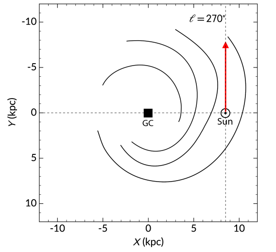
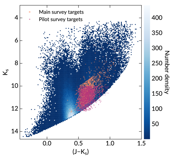
Figure 1: The location of observed fields and colour-magnitude selection of the GALAH main and pilot survey targets. Left panel: a schematic view of the Milky Way, illustrating the targeted line-of-sight. We observe along $\ell\approx 270^{\circ}$ and at five latitudes below the plane. The spiral arms are shown as traced by H ii gas, from Drimmel & Spergel (2001). Right panel: The colour-magnitude selection of the stars in this analysis is shown against all GALAH input catalogue targets within the observed region (including special bright targets). The pilot survey has a simple magnitude cut, at bright and faint limits of $K_{s}=10$ and $12$, respectively. The main GALAH survey magnitude selection $12<V_{JK}<14$ appears as a stripe in the ($J-K_{s}$) vs $K_{s}$ plane. The pilot survey extends slightly fainter than the main survey, and the handful of stars falling outside of the main survey selection are from a bright field.

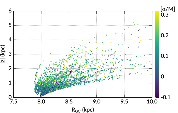
Figure 2: The distribution in Galactocentric radius and height below the plane for the entire sample, adopting R_GC,⊙ = 8 kpc. There are a few stars (not shown) outside the limits |z| $>6$ kpc and R $>10$ kpc. Stars are colour-coded by $\alpha$-abundances: low-$\alpha$ stars lie typically closer to the plane whereas $\alpha$-enhanced stars are found at greater distances from the plane.

We present in this paper results from the GALAH survey internal data release v1.3. The data acquisition and reduction are described in Martell et al. (2017) and Kos et al. (2017), respectively. The stellar parameter and abundance determination is summarised in Section 3.1. Briefly, GALAH spectra cover four optical bands, at wavelengths located within the Johnson-Cousins $B,V,R,I$ passbands, with resolving power $\lambda/\Delta\lambda\approx 28000$ (De Silva et al., 2015). The GALAH main-survey selects stars according to a simple magnitude criterion: $12<V_{JK}<14$, where the $V_{JK}$ magnitude is estimated from 2MASS (Skrutskie et al., 2006) $J,K_{s}$ photometry via the transformation:

$$V_{JK}=K_{s}+2(J-K_{s}+0.14)+0.382\,e^{\,(J-K_{s}-0.2)/0.50}$$ (1)

The above equation is discussed further in Sharma et al. (2018) (see their Fig. 1). The magnitude selection in $V_{JK}$ manifests as a $(J-K_{s})$ colour dependence when plotted as function of other magnitudes, as shown in Fig. 1, right panel.

In addition to normal survey fields which follow the $V_{JK}$ magnitude limit described above, GALAH also observed special fields, such as pilot survey fields (which included benchmark stars and clusters), and bright stars selected from the $Tycho$-2 catalogue (Martell et al., 2017), most of which also appear in the Gaia DR1 catalog (Brown et al., 2016).

As part of the GALAH pilot survey, we conducted a study of the chemical properties and distribution of the Galactic thin and thick disks. Fields were chosen towards Galactic longitude $\ell=270^{\circ}$, as shown in Fig. 1, left panel. This longitude was chosen to maximise the asymmetric drift component between thin and thick disk stars (Gilmore et al., 2002; Wyse et al., 2006), thus making it easier to distinguish them by their kinematics. We observed fields at five latitudes: $b=-16^{\circ},-22^{\circ},-28^{\circ},-34^{\circ}$ and $-42^{\circ}$. Fig. 2 shows the distribution of observed stars in Galactic coordinates $R_{\mathrm{GC}}$ and $|z|$ (distances are derived as per Section 3.2). Adopting $R_{\mathrm{GC},\odot}=8$ kpc, most of the stars are concentrated around the solar radius, between $R_{\mathrm{GC}}=8-8.5$ kpc, and up to about 4 kpc in height below the Galactic plane. Since our longitude range is between $\ell=(260,280)$, we also observed stars with $R_{\mathrm{GC}}<8$ kpc.

We chose to use only giants in this study to include a larger range of distances and heights from the plane. The magnitude limits of the main GALAH survey result in giants making up only about $25$% of stars observed. In order to increase the fraction of giants, a colour cut at $(J-K_{s})>0.45$ was imposed for the pilot survey prior to observations, which excludes turn-off stars and some dwarfs. We also extended the faint $V_{JK}$-magnitude limit of the pilot survey to 14.5 in order to observe a larger fraction of clump giants. Also included in this analysis are giants from the GALAH main-survey that fall within the same Galactic longitude–latitude range described above. The colour and magnitude selection for all stars included in the analysis is shown in Fig. 1.

3 Data analysis

3.1 Stellar parameters and alpha abundances

The GALAH stellar parameters and abundances pipeline will be described in detail elsewhere; here we seek to give a brief summary. The pipeline is a two-step process, involving spectral synthesis using SME (Spectroscopy Made Easy)  (Valenti & Piskunov, 1996; Piskunov & Valenti, 2017) and the data-driven generative modelling approach of The Cannon (Ness et al., 2015). We identify a sample of stars with high signal-to-noise ratio, each visually inspected to be free of irregularities like unexpected continuum variations and large cosmic ray residuals. This set of stars serves as the training set, the labels of which are propagated to all other survey stars. The training set includes $Gaia$ benchmark standards (Jofré et al., 2014; Heiter et al., 2015) whose parameters have been determined by non-spectroscopic methods; globular and open clusters and stars with accurate asteroseismic surface gravity from K2 Campaign 1 (Stello et al., 2017). In total there are $\approx$2500 training stars.

In the first step, stellar parameters for the training set are obtained with SME. Here we use the marcs model atmospheres (Gustafsson et al., 2008), and non-LTE corrections for Fe (Lind et al., 2012). SME syntheses of H$\alpha$ and H$\beta$, neutral and ionised lines of Ti, Sc and Fe are used to determine $T_{\textrm{eff}}$, $\log g$, [M/H], v_mic (micro turbulence) and $V\sin i$ (rotational velocity), converging at the global minimum $\chi^{2}$. The stellar parameters are fixed when individual abundances are computed for the $\alpha$-elements Mg, Si, Ti. The weighted average of these elements gives [$\alpha$/M], and all abundances are scaled according to the Solar chemical composition of Grevesse et al. (2007).

Although the GALAH wavelength range includes lines of the $\alpha$-elements Ca and O, they are currently omitted from the weighted average because the Ca lines fall within problematic spectral regions (due to bad CCD pixels and/or sub-optimal data reduction), and the O i triplet at 7772–7775 Å is subjected to large non-LTE effects (Amarsi et al., 2015, 2016), which are not yet accounted for in the GALAH analysis pipeline. Relative to $Gaia$ benchmark standards, SME produces accurate results with offsets in $\log g$ and [M/H] of $-0.15$ and $-0.1$ dex respectively, in the sense that it underestimates these values. The same surface gravity offset is also observed when SME results are compared to asteroseismic $\log g$ obtained with oscillations from Stello et al. (2017). The offsets are constant across the HR diagram, and are corrected by simply adding 0.15 and 0.1 dex to all $\log g$ and [M/H] values of the training set prior to parameter propagation with The Cannon (Sharma et al., 2018).

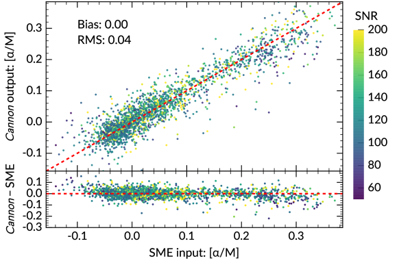
Figure 3: Cross-validation of The Cannon-output against SME input for the label [$\alpha$/M]. Stars are colour coded by signal-to-noise ratios in the ‘green’ arm of HERMES, the wavelength of which lies within the Johnson-Cousins V-band. The top panel shows the 1:1 relation between SME input and The Cannon output. The bottom panel shows the distribution of the difference. The Cannon reproduces the SME input without bias, and to 0.04 dex precision.

In the second step, The Cannon learns the training set parameters and abundances (labels) from SME, and builds a quadratic model at each pixel of the normalised spectrum as a function of the labels (Ness et al., 2015). This model is then used to determine stellar parameters and abundances for all other survey spectra. In addition to the six primary labels described above, The Cannon uses a seventh label, extinction $A(K_{s})$, to minimise the effect of reddening and diffuse interstellar bands on [$\alpha$/M] determination. The extinction for each star of the training set was estimated with the RJCE method (Majewski et al., 2011). We used 2MASS $H$-band and WISE 4.5 $\mu$m photometry (Wright et al., 2010), following procedures outlined in Zasowski et al. (2013). Parameter errors are estimated by cross-validating the input (SME) and output labels (The Cannon) for the training set. Cross-validation was done by partitioning the reference set into unique sub-samples, each consisting 20% of the full set. Five tests were performed, each time a 20% sub-sample is left out of the training step, and used only to validate the results. Fig. 3 shows the combined cross-validation outcomes of all five tests for label [$\alpha$/M]. The training set results have also been successfully applied to the TESS-HERMES survey, and the error estimation of stellar labels except for [$\alpha$/M] is shown in Fig. 5 of Sharma et al. (2018). Overall, The Cannon achieves internal precisions of 47 K in $T_{\textrm{eff}}$, 0.13 dex in $\log g$, 0.05 dex in [M/H] and 0.04 dex in [$\alpha$/M], which are typical of the errors reported in this data release.

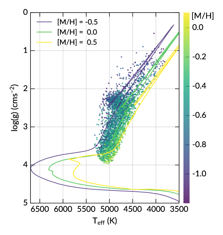
Figure 4: The Kiel diagram from The Cannon for the sample of stars in this analysis, colour coded by [M/H]. Over plotted are 4 Gyr parsec isochrones at metallicities indicated in the figure legend. The stellar parameters behave as predicted by the evolutionary tracks after bias corrections to The Cannon training set (see text for details).

Fig. 4 shows The Cannon-derived stellar parameters for the full sample of giants selected for analysis. We have excluded most sub-giants, turn-off and main-sequence stars. The Cannon is able to reproduce the accuracy and precision of SME such that all parameters follow the parsec isochrone tracks (Marigo et al., 2017) without further calibrations. The [$\alpha$/M]–[M/H] plot is shown in Fig. 5 for a sub-sample of stars with signal-to-noise ratio $\geq$ 80 per resolution element. We observe the two distinct $\alpha$-tracks in the [$\alpha$/M]–[M/H] plane: a low-$\alpha$ track extending from [M/H] $\approx$ 0.4 to $-0.6$, usually defined as the chemical thin disk, and a high-$\alpha$ track extending from [M/H] $\approx-0.2$ to $-1$, usually defined as the chemical thick disk. The typical precision of the [$\alpha$/M] measurements is 0.04 dex, similar to that of [M/H].

We do not include stars with [M/H] $\leq-1$ dex here, because few metal-poor stars could be used in the training set (the stars are rare, and typically have low SNR), rendering The Cannon results for metal-poor stars significantly less accurate. The Cannon has limited ability to extrapolate, which is evident in the comparison to $Gaia$ benchmarks: stars with [M/H] $<-1$ have larger deviations from reference values (Sharma et al., 2018). This does, however, exclude the metal-weak thick disk from our analysis. We find that other studies which include the metal-poor extension of the thick disk, such as Katz et al. (2011); Ruchti et al. (2011) reported similar results to ours (see detailed discussion in Sections 5.2.2 and 6). Furthermore, there are few stars with [M/H] $\leq-1$ dex to begin with (2% of the full sample), so their exclusion may have small effects on the vertical gradients derived in later sections, but it is unlikely that this would have a major impact on our conclusions.

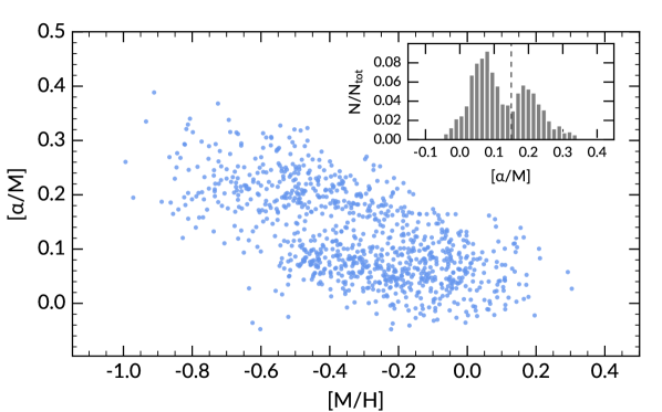
Figure 5: $\alpha$-abundances as a function of metallicity for a sub-sample with signal-to-noise $\geq$ 80 per resolution element. There are two distinct abundance sequences corresponding to the thin disk (low-$\alpha$) and the thick disk (high-$\alpha$). Inset: histogram of the [$\alpha$/M] distribution, the dotted line indicate [$\alpha$/M] = 0.15, where the two populations appear to separate.

3.2 Distance determination

Distances are typically determined by isochrone fitting methods using the fundamental stellar parameters $T_{\textrm{eff}}$, $\log g$ and [M/H] and photometry. Theoretical constraints, such as stellar evolution and initial mass functions (IMF) have been included by Zwitter et al. (2010) and Burnett & Binney (2010), respectively, to obtain more accurate distances for the RAVE survey (Steinmetz et al., 2006). Isochrone distances are dependent on all fundamental parameters, but a strong dependence on [M/H] can cause correlated errors when trying to assess the metallicity distribution as a function of distance from the Galactic centre or above the plane (Schlesinger et al., 2014; Anguiano et al., 2015). In this section we describe an empirical method of distance determination that does not have such a strong dependence on inferred [M/H], which may be advantageous for our measurements of metallicity vertical gradients in Section 5.

To determine the distance, we exploit the relationship between stellar surface gravity and radius $R$ using Kepler asteroseismic data from Casagrande et al. (2014). Fig. 6 shows the $\log g-R$ correlation and the exponential function that best fits the data. Using spectroscopically determined $\log g$, we compute for each GALAH star a radius (in solar radii) using the function:

$$R_{*}=165(0.33^{\log g})$$ (2)

Note that starting from the definition of $g=GM/R_{*}^{2}$, where $G$ is the gravitational constant, and $M$ the mass of the star, we arrive at the formula:

$$R_{*}/R_{\odot}=10^{0.5(\log g_{\odot}-\log g)},$$ (3)

which is equivalent to $165.59*0.316^{\log g}$, assuming that $M=M_{\odot}$ and the solar $\log g$ is 4.438068 cm $\mathrm{s}^{-2}$ . However, the function used to fit the data in Fig 6 returns the minimum reduced-$\chi^{2}$ (perhaps due to differences in the stellar mass compared to the assumed solar value), and is used instead.

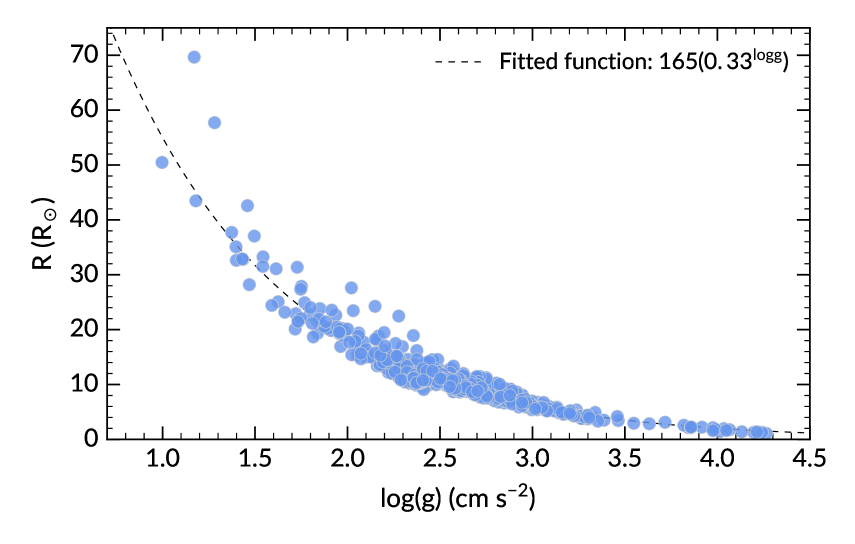
Figure 6: The correlation between stellar surface gravity and radius, data from the Kepler sample of Casagrande et al. (2014). The stellar radius as a function of $\log g$ is best described by an exponential.

The absolute luminosity is estimated using the effective temperature and radius relation:

$$L=4\pi R_{*}^{2}\sigma T_{\textrm{eff}}^{4}$$ (4)

Finally, we interpolate the stellar parameters $T_{\textrm{eff}}$, $\log g$, [M/H] over a grid of synthetic spectra to determine the correction that needs to be applied to 2MASS $J,H,K_{s}$ photometry to derive the bolometric flux $\mathcal{F}_{bol}$. We correct for extinction using the Schlegel et al. (1998) map to de-redden the observed 2MASS magnitudes. This is done using extinction coefficients computed on-the-fly for the set of stellar parameters adopted (Casagrande et al., 2010). The distance is then simply:

$$D=\left(\frac{L}{4\pi\mathcal{F}_{bol}}\right)^{1/2}$$ (5)

As is evident from Fig. 6, the $\log g$–stellar radius relation is poorly constrained for $\log g\leq 1.5$, because we have few seismic data points in this region and the scatter is larger. There are however relatively few stars with $\log g<1.5$ in our sample (see Fig. 4).

3.2.1 Distance error estimate

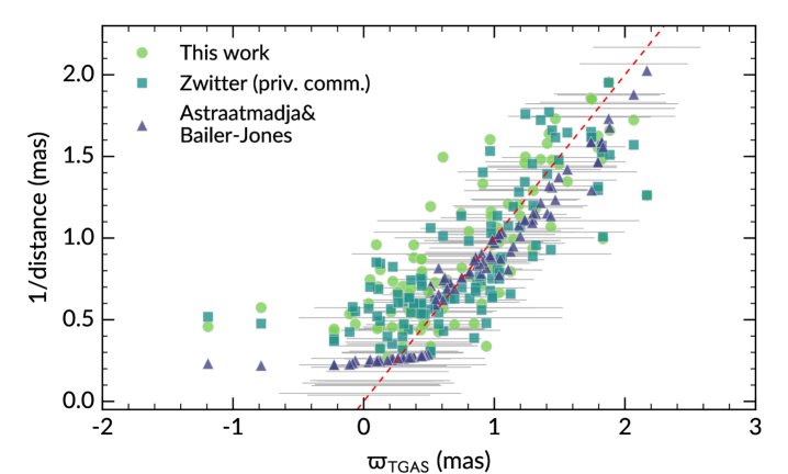
Figure 7: Comparison of distances derived from GALAH stellar parameters (this work/Zwitter) and Bayesian TGAS distances (Astraatmadja & Bailer-Jones). On the $x$-axis are TGAS parallaxes, and the grey horizontal bars indicate reported uncertainties (including systematic errors). There is a break in the Astraatmadja & Bailer-Jones (2016) values because a different prior is used for $\varpi<$ 0.5 mas, which according to the authors is more accurate for large distances (see text for details). The $y$-axis shows inferred parallaxes from the three distance methods. The dashed line is the 1:1 correlation. As the parallax decreases, TGAS fractional errors become very large, and in some cases negative parallaxes are reported. Compared to TGAS, distances derived from GALAH stellar parameters have an overall scatter of $\approx 0.37$ mas, which is within the typical TGAS uncertainty of 0.3 mas. For $\varpi<$ 0.5 mas, there is a systematic offset between TGAS and IRFM/Zwitter distances of $\approx 0.3$ mas.

We tested the accuracy and precision of our distance determination method by comparing our results to the first $Gaia$ data release (Brown et al., 2016, TGAS), which provides accurate parallaxes ($\varpi$) for bright stars in the $Tycho$-2 catalogue (Michalik et al., 2015). Because of the brighter magnitude limit of $Tycho$-2, we only have a small overlap of about $100$ stars for comparison. We also compare our distances to those of Astraatmadja & Bailer-Jones (2016), who computed Bayesian distances using TGAS parallaxes and Milky Way density models. Finally, we include a comparison between our method and that of Zwitter et al. (2010), which computes the distance modulus by fitting stellar parameters to their most likely isochrone counterparts.

Fig. 7 compares the unaltered TGAS parallaxes with the inferred parallaxes from the three distance methods. Distances from Astraatmadja & Bailer-Jones (2016) are median values of the posterior from their Milky Way density model. However, they note that the Milky Way model under-estimates distances for $\varpi<0.5$ mas when compared to Cepheid distances, as the model assumes that a star is more likely to be in the disk and photometric information is not used. Thus, the distances used here for $\varpi<0.5$ are the median of the posterior from their exponentially decreasing density model with scale length $L=1.35$ kpc (Astraatmadja & Bailer-Jones, 2016).

The comparison shows no systematic discrepancy for $\varpi_{\textrm{TGAS}}>0.5$ mas. The distances computed from our IRFM and the Zwitter et al. (2010) isochrone fitting method using the same spectroscopic parameters agree to within $\approx$$15$%. Compared to TGAS, both the IRFM and isochrone fitting method have a standard deviation of $0.3$ mas, which is well within the typical errors quoted for TGAS parallaxes. We noticed that the Bayesian distances from Astraatmadja & Bailer-Jones (2016) are slightly over-estimated compared to TGAS between $\varpi_{\textrm{TGAS}}$ = 1–2 mas.

We do find an offset between all distance methods and the TGAS parallaxes for $\varpi_{\textrm{TGAS}}$ = 0–0.5 mas, where the TGAS values may be underestimated. For stars with $\varpi_{\textrm{TGAS}}>0$, the offset is 0.33 mas for the spectroscopic distances. Stassun & Torres (2016) found a similar offset, between TGAS and inferred parallaxes derived from eclipsing binaries, however their results are applicable only to smaller distances, which is not seen in our results (see also Huber et al. 2017). A likely reason for the GALAH-TGAS offset is that TGAS uncertainties becomes very large at $\varpi<0.5$ mas, so for a magnitude-limited sample, TGAS systematically scatters to smaller values.

In summary, we find that our distances are accurate compared to TGAS parallaxes and the Bayesian distances of Astraatmadja & Bailer-Jones (2016), albeit with an offset for $\varpi_{\textrm{TGAS}}<0.5$ mas. Overall the standard deviation between the two spectroscopic methods is $17$%. Since both our method and the isochrone fitting method used the same set of stellar parameters, the comparison between them is indicative of their intrinsic uncertainties. Assuming that both methods contribute equally to the overall scatter, the internal uncertainty of each method is 12%. This is the value we adopted as the our distance errors.

3.3 Separating the thin and thick disk populations

High resolution spectroscopic studies show that the $\alpha$-enhancement of local disk stars follow two distinct tracks (e.g., Bensby et al. 2014; Adibekyan et al. 2011). The high-$\alpha$ population is typically associated with the thick disk and has high velocity dispersion; the low-$\alpha$ stars are associated with the thin disk, with low velocity dispersion. The thick disk also has a larger rotational lag compared to the thin disk.

The thick disk can also be defined geometrically by star counts (Jurić et al., 2008; Chen et al., 2011), or by metallicity and kinematics (Katz et al., 2011; Kordopatis et al., 2011). The thin and thick disks do overlap in their spatial, metallicity and kinematical distributions. Because of the two distinct sequences in [$\alpha$/M]-[Fe/H] space, definition of the thick disk by its enhanced $\alpha$-abundances relative to thin disk stars of the same metallicity is currently widely used (Adibekyan et al., 2013; Bensby et al., 2014; Haywood et al., 2015) . However, the adopted dividing line between the high and low-$\alpha$ populations differs from author to author. Furthermore, some stars with thick disk chemistry have thin disk kinematics, and there are stars that lie in the intermediate region between the two [$\alpha$/M] sequences. The ‘thick disk’ population that we are interested in is the stellar fossil of the turbulent epoch of fast star formation at high-$z$. Following this definition, we want to exclude the flaring outer thin disk, which contributes to the geometrical thick disk, and metal-rich stars which may have migrated from the inner thin disk.

To this end, we chose to separate the two components by fitting a mixture of Gaussian distributions using the Expectation-Minimisation algorithm (Dempster et al., 1977). We use three variables: [M/H] and [$\alpha$/M] and the radial velocity (RV), which, to the best of our knowledge, has not been done previously. At $\ell=270^{\circ}$, the component of the rotational lag between the thin and thick disk along the line-of-sight is maximised for most of our fields, such that RV is a good proxy for $V$ velocity (see also Kordopatis et al. 2017). Instead of using the Cartesian $V$ space velocity component, which has significant proper motion errors, we use the precise GALAH radial velocity to help separate the two populations (98% of our survey stars have RV uncertainty $<0.6$ kms^-1 according to Martell et al. 2017).

The python scikit-learn (Pedregosa et al., 2011) module GaussianMixture was used to perform the fitting. we assume that the data cube can be described by 2 multivariate Gaussians, each characterised by its three means and $3\times 3$ covariance matrix: $\theta_{j}=(\mu_{j},\Sigma_{j})$, where $j=\{1,2\}$, to represent the low and high-$\alpha$ sequences. Note that Rojas-Arriagada et al. (2016) argue the [$\alpha$/M] vs [M/H] distribution could be described by five components, but here we are not concerned with finding sub-components of the two $\alpha$-sequences.

Given a set of data ($x_{1},x_{2},...,x_{n}$), the likelihood function is defined as:

$$\mathcal{L}(\theta;x)=\prod_{i=1}^{n}\sum_{j=1}^{2}w_{j}f(x_{i};\mu_{j},\Sigma_{j}),$$ (6)

where $f$ is the probability density function of a multi-variate normal distribution and $w_{j}$ is the weight of each distribution. The algorithm initialises with random guesses for $\theta=(w_{j},\mu_{j},\Sigma_{j})$ and iterates until the log-likelihood is at minimum. The probability that a data point $x_{i}$ belongs to component $j$ is given by:

$$P_{j}\,(x_{i}\,|\,\theta)=\frac{w_{j}f(x_{i};\mu_{j},\Sigma_{j})}{w_{1}f(x_{i};\mu_{1},\Sigma_{1})+w_{2}f(x_{i},\mu_{2},\Sigma_{2})}$$ (7)

where

$$P_{1}(x_{i})+P_{2}(x_{i})=1$$ (8)

Fig. 8 shows projections in the [$\alpha$/M]–[M/H] and the RV–[$\alpha$/M] planes, where two Gaussian components centred at [$\alpha$/M] = 0.05 and [$\alpha$/M] = 0.2 can be seen, each with a distinctive median radial velocity. Stars are colour-coded by their thick disk probability. As expected, the high-$\alpha$ stars have much higher thick disk probability than the low-$\alpha$ stars. It is also apparent that stars with [M/H] between $-0.4$ and 0 are likely to be designated thin disk membership, because their radial velocities and metallicity more closely resemble that of thin disk stars. This is perhaps the most important distinction between our ‘thick disk’ definition and that of other studies: that the overall more $\alpha$-enhanced population does not include the high metallicity, high-$\alpha$ population. This places important constraints on subsequent analyses and the interpretation of our results with respect to models of disk formation, as here we are assuming that the thick disk is almost exclusively old by excluding more metal-rich stars.

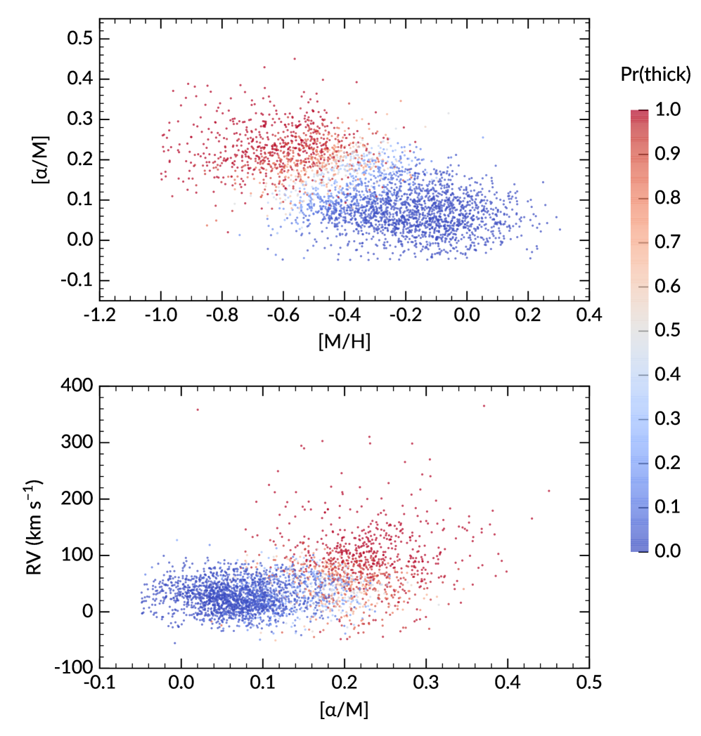
Figure 8: Results of the Gaussian mixture decomposition. Top panel: projection along the [$\alpha$/M]–[M/H] plane. Bottom panel: projection along the [$\alpha$/M]–RV plane, both colour-coded by the probability of a star belong to the thick disk. We can see that there are two well defined populations in both projections, however there are also plenty of stars that are difficult to place in either population. These stars have chemistry and kinematics that could belong to either of the classically defined ‘thin’ and ‘thick’ disk. Stars that are typically defined as thin disk by chemistry have Pr(thick) $\leq$ 0.1. Stars with typical thick disk chemistry however have a higher velocity dispersion and therefore a larger spread in probability, ranging from 0.6 $\leq$ Pr(thick) $<1$.

Furthermore, Fig 8 indicates that there are ‘transition stars’, which have higher [$\alpha$/M] than thin disk stars at the same metallicity and kinematics that lie between the two disks, making it is difficult to assign them to either population. We therefore assigned thin disk membership only to stars that have thick disk probability $\leq 0.1$, which have [$\alpha$/M] $\leq 0.15$, consistent with the location of the ‘gap’ between high and low $\alpha$ populations for our data set. The majority of stars with thick disk probability between 0.1–0.5 have [$\alpha$/M] values between 0.15–0.3 dex. These ‘transition’ stars are omitted from the analysis to minimise contamination in each defined population. Approximately 13% of the overall sample are in the ‘transition’ category.

4 Selection bias

Fig. 1, right panel, shows that the pilot survey has a simple magnitude cut, 10 $<K_{s}$ $<$ 12, while the main survey colour-magnitude selection appears to be a stripe in the $(J-K_{s})_{0}$ vs $K_{s}$ plane, from the criterion that $12<V_{JK}<14$. The main survey also observed some bright stars that fall outside the lower magnitude limit. In addition, the pilot survey purposely observed a larger fraction of stars at higher latitudes, which means that the population at low latitudes is under-represented. These selection biases affect the resulting metallicity, distance (and therefore vertical height) distributions of the observed population. In this section we aim to correct for these effects so that the underlying Galactic population can be correctly recovered.

4.1 Correcting for selection effects

4.1.1 Field selection bias

The first selection effect that we corrected was the bias from targeting particular fields. We purposely observed a larger relative fraction of stars at higher latitudes to target the thick disk, and thus biased against low latitude stars.

To correct for this, we determined for each field the number of stars present in the observed sample compared with the number of photometric targets available for that field in the GALAH input catalogue, within the same magnitude limit, e.g.:

$$w_{field}=\frac{N_{observed}\ (12<{V}_{JK}<14)}{N_{targets}\ \ (12<{V}_{JK}<14)}$$

We dealt with the magnitude ranges of the pilot and main surveys separately. The limits used are 12 $<$ V_JK $<$ 14 for main survey fields; 12 $<$ V${}_{{JK}}<$14.5 for pilot fields and 9 $<$ V_JK $<$ 12 for the bright field.

4.1.2 Magnitude and colour selection bias

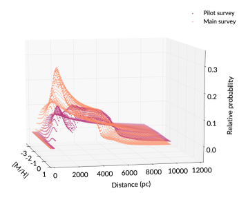
Figure 9: The relative probability of observing a particular star in the metallicity-distance plane given the colour-magnitude selection of GALAH pilot and main surveys. While we show the metallicity distribution up to [M/H]=$-$3 dex, we do not have any stars with [M/H] $<$ $-$1 in our sample. The distance distribution is most affected by the colour-magnitude selection of the two surveys, with the pilot survey favouring more distant stars. The metallicity of both surveys peaks around solar, but compared to the main survey, the pilot survey has a larger fraction of stars that are more metal-poor.

Following Casagrande et al. (2016), we assessed the magnitude and colour selection bias by creating a synthetic population using BaSTI isochrones (Pietrinferni et al., 2004). From a data cube that spans 0.5 to 10 Gyr in age, $-3$ to 0.5 dex in metallicity and 10 to 10000 pc in distance, each point in the age and metallicity plane is populated on the isochrones according to the Salpeter (1955) IMF, with the distances providing apparent magnitudes for each population. We then applied the same apparent colour and magnitude cut as shown in Fig. 1 to obtain the ratio of stars observed with our selection function compared to the total number of stars that populate a given point in the age, metallicity and distance cube. As in the previous section, the pilot and main survey selection functions are taken into account separately. Because there is no age information available for this sample, we integrated the observed probabilities over all ages for each point in the distance–metallicity plane. This implicitly assumes that the age distribution is flat in the solar neighbourhood (e.g., Edvardsson et al. 1993; Ting et al. 2015). With this method, the effects of different evolutionary time-scales of each stellar population on the HR diagram are also taken into account via the IMF.

Fig. 9 shows the relative fraction of stars observed after the colour-magnitude selection is applied. The most metal-poor and metal-rich stars are slightly biased against, similarly so for both the pilot and main survey selections. The distances, on the other hand, are very different for the pilot and main surveys. The main survey is biased against stars more distant than 1.5 kpc, especially at lower metallicities. The pilot survey observes relatively more distant (and thus larger $|z|$) stars as intended. In addition, the pilot survey colour and magnitude limit particularly targetted red clump stars, which primarily contributed to the second peak in its selection function.

The relative ratios obtained from this population synthesis method are dependent on the choice of stellar models and IMF, however we note that we are only using these numbers in the relative sense, to gauge the importance of one star compared to another. In this sense, we do not expect the selection effects to change qualitatively.

4.2 Effects of bias correction

The final weight is determined by combining the fraction from field selection bias and the isochrone population synthesis. Since the fraction indicates how likely a star is observed, the weights are computed as

$$w_{final}=\frac{1}{w_{field}\times w_{isochrone}}$$

so that stars less likely to be observed are given higher weights.

Overall, the corrections mean that more metal-poor and distant stars are weighted more heavily. Effects of the weights on the [M/H] and $|z|$ distributions are shown in Fig. 10.

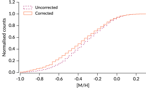
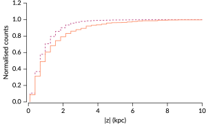
Figure 10: Cumulative histograms showing bias-uncorrected and corrected metallicity and height $|z|$ distributions. Left panel: [M/H] distribution. Right panel: height distribution. Typically the corrections account for the bias against stars that are more metal-poor and further from the plane.

4.3 Halo contamination

To assess the halo contamination in our low and high-$\alpha$ samples, we used the Galaxia code (Sharma et al., 2011), based on the Besançon models (Robin et al., 2003) to synthesise the stellar population within our observed region. We applied the same colour-magnitude limits (in 2MASS $J,K_{s}$ photometry as shown in Fig. 1) for the pilot and main survey samples separately. The simulation shows that within our metallicity range $(-1\leq$ [M/H] $\leq 0.4)$, the contamination of halo stars is extremely small, at 0.5% for both of the pilot and main surveys. Therefore, any effects of halo stars on our results would be negligible.

5 Metallicity profiles

5.1 Radial metallicity profiles

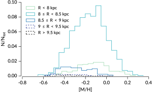
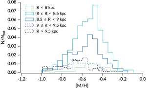
Figure 11: Radial distribution of the thin (low-$\alpha$) and thick (high-$\alpha$) disks, after correcting for selection effects. Left panel: the thin disk’s mean metallicity changes rapidly as a function of radial distance. This is due to both the radial metallicity gradient observed in the thin disk, and that the average vertical height increases with increasing radial distance. Right panel: The thick disk, on the other hand, does not show a strong change in shape nor median value with radial distance.

In figure 11 we show the MDF of the thin and thick disks in radial distance bins of 500 pc. Within the small range that we cover, no metallicity gradient is observed for the thick disk. The MDF remains constant in shape and median value across all radial distances up to 9 kpc, which is consistent with Hayden et al. (2015). Beyond 9 kpc, we notice that the MDF skews slightly towards more metal-poor values, but we interpret this as an effect caused by observing progressively larger median $|z|$ as we move further from the Galactic centre (see Fig. 2) rather than the thick disk having a radial metallicity gradient.

For the low-$\alpha$ population, we observe only a small number of stars at radial distances further than 9 kpc. The distribution is roughly Gaussian at all locations, but skews towards metal-poor with increasing $R$. In Fig. 2, it is evident that the majority of $\alpha$-poor stars (thin disk) are confined to the plane. At $R_{\mathrm{GC}}=8.5$ kpc, most of the stars lie above |$z$| = 1 kpc, so here we are likely to be observing only the metal-poor tail of the thin disk. The shift towards lower metallicity at large $R$ is likely due to the radial metallicity gradient of the thin disk (Cheng et al., 2012; Genovali et al., 2014; Hayden et al., 2015), and the vertical gradient discussed in the next section.

Table 1: The mean (and standard error), dispersion and skewness of the metallicity distributions at different radial bins for the low-$\alpha$ population.

Radial range	Mean [M/H]	Standard deviation	Skewness
R $<$ 8 kpc	$-0.12\pm 0.01$	0.15	$+0.01\pm 0.02$
8 $\leq$ R $<$ 8.5 kpc	$-0.16\pm 0.004$	0.16	$-0.02\pm 0.01$
8.5 $\leq$ R $<$ 9 kpc	$-0.30\pm 0.01$	0.13	$+0.30\pm 0.02$
9 $\leq$ R $<$ 9.5 kpc	$-0.37\pm 0.03$	0.17	$+1.50\pm 0.07$
R $>$ 9.5 kpc	$-0.42\pm 0.05$	0.13	$-0.30\pm 0.07$

Table 2: The mean (and standard error), dispersion and skewness of the metallicity distributions at different radial bins for the high-$\alpha$ population.

Radial range	Mean [M/H]	Standard deviation	Skewness
R $<$ 8 kpc	$-0.52\pm 0.02$	0.13	$-0.79\pm 0.04$
8 $\leq$ R $<$ 8.5 kpc	$-0.53\pm 0.01$	0.15	$-0.27\pm 0.01$
8.5 $\leq$ R $<$ 9 kpc	$-0.57\pm 0.01$	0.15	$-0.26\pm 0.02$
9 $\leq$ R $<$ 9.5 kpc	$-0.61\pm 0.01$	0.14	$-0.36\pm 0.03$
R $>$ 9.5 kpc	$-0.70\pm 0.02$	0.15	$-0.07\pm 0.04$

We provide the median, standard deviation and skewness of each radial bin of each population in tables 1 and 2. These support our conclusions that the MDFs of both populations within our $R_{\mathrm{GC}}$ range are close to Gaussian, and that there is little change in the mean metallicity and shape of the high-$\alpha$ population. We caution that the statistics is more uncertain for bins $R_{\mathrm{GC}}>9$ kpc of the low-$\alpha$ population due to the small sample size.

5.2 Vertical metallicity profiles

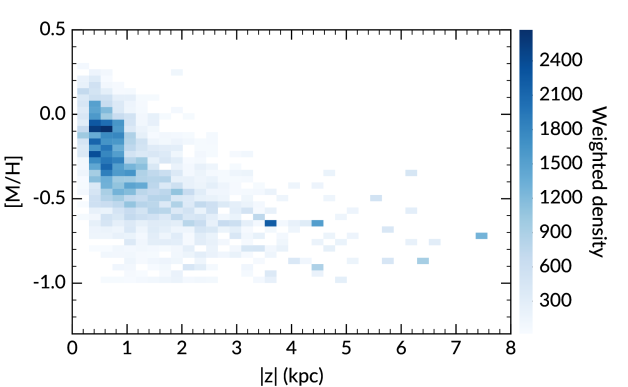
Figure 12: Variation of metallicity with distance from the Galactic plane for all stars independently of their alpha assignment (the ‘transition’ stars mentioned in Section 3.3 are also included). The density was weighted using bias correction fractions described in Section 4. The metallicity decreases smoothly with increasing height, however the gradient appears to flatten at |z| = 2 kpc.

The vertical gradients were measured using an orthogonal linear least squares regression to all data points, taking into account each data point’s uncertainties in [M/H] and vertical height. Each point is then weighted by the selection bias correction described in Section 4. We do this by decreasing the uncertainty of each data point by the square root of the correction factor. In this section we report the gradients measured for the disk as a whole, and for each defined $\alpha$ sub-population. The gradients measured are summarised in Table 3.

Fig. 12 shows a density plot of the metallicity as a function of height above the plane for all stars, including those that were omitted from the individual $\alpha$-subpopulation, as explained in Section 3.3. The density was weighted to correct for selection biases using relative fractions described in Section 4. We observe that the metallicity decreases smoothly as $|z|$ increases. The vertical gradient for the disk overall is d[M/H]/d$z=-0.22\pm 0.01$ dex kpc^-1, and appears to flatten at larger $|z|$, from about $|z|=2$ kpc. The gradient value is in good agreement with overall disk gradients measured by Schlesinger et al. (2014) for a sample of volume-complete SEGUE dwarfs.

For each of the sub-populations, we also found a metallicity gradient, as shown in Fig. 13. Over-plotted in each panel are averaged values of metallicity at different $|z|$ bins for clarity, but these binned values have no effect on the data fitting. We discuss the vertical gradients below.

5.2.1 The low-$\alpha$ population

The low-$\alpha$ population, or thin disk, is known to have a radial metallicity gradient d[M/H]/d$R$ of $\approx$$-0.08$ dex kpc^-1, which flattens at progressively higher $|z|$ (Cheng et al., 2012; Hayden et al., 2014). The radial metallicity gradient can be seen in the left panel of Fig. 11, where the median metallicity shifts to lower values at larger $R_{\textrm{GC}}$. The small $R_{\textrm{GC}}$ range that we cover does not allow us to reliably measure radial metallicity gradients, so we corrected for this effect by estimating the metallicity of each star at $R=8$ kpc using radial gradients specified in Cheng et al. (2012) for height bins $0.25<|z|<0.5$ kpc; $0.5<|z|<1$ kpc and $1<|z|<1.5$ kpc. The data set of Cheng et al. (2012) did not extend beyond $|z|$ = 1.5 kpc, so for all heights above this value, we assumed the same radial gradient as at $1<|z|<1.5$. Overall, the radial gradient correction caused a change of $-0.01$ dex kpc^-1in the vertical gradient. The final weighted vertical gradient of the low-$\alpha$ population d[M/H]/d$z$ = $-0.18\pm 0.01$ dex kpc^-1.

Studies that were conducted prior to recent large spectroscopic surveys typically reported steeper negative gradients than our value. Bartašiūtė et al. (2003) separated thin disk stars by rotational lag and measured $-0.23\pm 0.04$ dex kpc^-1. Marsakov & Borkova (2006) used both space velocities and orbital eccentricities restrictions to select thin disk stars and reported a gradient of $-0.29\pm 0.06$ dex kpc^-1. It is highly likely that separating the thin disk purely based on kinematics would result in contamination of thick disk stars, which explains why these gradients are in agreement with our overall disk gradient, but steeper than the gradient of the low-$\alpha$ population.

Few studies of disk vertical metallicity gradients separated the thin/thick disk using chemistry. The only recent studies that identified the thin disk by their $\alpha$-abundances are Schlesinger et al. (2014) (SEGUE), Hayden et al. (2014) (APOGEE) and Mikolaitis et al. (2014) (Gaia-ESO). Hayden et al. (2014) found a low-$\alpha$ gradient of $-0.21\pm 0.02$ dex kpc^-1 at the solar circle for the APOGEE DR10 sample, which is slightly steeper than our value. Hayden et al. (2014) also correct for the radial metallicity gradient, using values similar to that of Cheng et al. (2012) used here. The small discrepancy could arise from our different definitions of the thin disk, as Hayden et al. (2014) made a straight-line cut at [$\alpha$/M] = 0.18. In Fig. 6 of Hayden et al. (2014), their low-$\alpha$ population extends to [M/H] = $-2$ dex while ours extends to only [M/H] = $-0.6$ dex. The low-$\alpha$, very metal-poor stars seen in APOGEE data could belong to the halo (Nissen & Schuster, 2010; Adibekyan et al., 2013), and this contamination would steepen the gradient.

Schlesinger et al. (2014) also computed a gradient for the low-$\alpha$ population of SEGUE dwarfs. They measured, for the disk as a whole, a vertical metallicity gradient of $-0.24^{+0.04}_{-0.05}$ dex kpc^-1, which is in agreement with our measurement. However their low-$\alpha$ population has a gradient consistent with zero: d[M/H]/d$z=-0.01^{+0.09}_{-0.06}$ dex kpc^-1. However, their intermediate $\alpha$ sub-population with $0.2<$[$\alpha$/M]$<0.3$ has d[M/H]/d$z=-0.17^{+0.08}_{-0.07}$ dex kpc^-1, which agrees with our low-$\alpha$ metallicity gradient. We thus conclude that the discrepancy between our result and that of Schlesinger et al. (2014) is largely due to the chemical separation criteria (also see Ciucǎ et al. 2018, who found an age-dependence for the thin disk vertically metallicity gradient, such that the youngest population has a flatter gradient).

Mikolaitis et al. (2014) measured a slightly shallower gradient of d[M/H]/d$z=-0.11\pm 0.01$ for Gaia-ESO dwarfs and giants. The Gaia-ESO sample is more metal-poor overall and Mikolaitis et al. (2014) separated thick disk stars by the location of under-densities in their [Mg i/M] histograms (their Fig. 3). The dividing line is at different values of [Mg i/M] for different metallicity regimes. In Fig. 10 of Mikolaitis et al. (2014), it is clear that their sample is biased against metal-rich stars, such that there are very few stars with [M/H]$>0$ (also see Stonkutė et al. 2016).

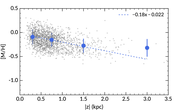
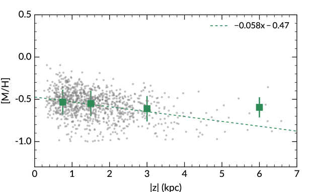
Figure 13: Variation of metallicity with distance from the Galactic plane for each $\alpha$ sub-population. Top panel: the thin disk has a steep negative gradient, which is consistent with what many authors have observed previously. Bottom panel: the thick disk has a shallower gradient. The trends are fitted over grey data points, over-plotted are averaged values of four height bins and their one sigma error bars. It is important to note that the binned values were not used in the gradient fitting.

5.2.2 The high-$\alpha$ population

The vertical metallicity distribution of the thick disk (high-$\alpha$) stars, is relatively flat compared to the low-$\alpha$ population, at $-0.058\pm 0.003$ dex kpc^-1. Several authors have measured the vertical gradient for the thick disk, using different methods to define this population. Earlier studies, such as Gilmore et al. (1995) and Prieto et al. (2006), reported no vertical metallicity gradient in the thick disk (Prieto et al. 2006 quoted an upper limit of d[M/H]/d$z=0.03$ dex kpc^-1). More recently, Boeche et al. (2014) concluded that the vertical metallicity gradient of the thick disk is consistent with zero, based on a sample of RAVE giants. However, other studies, using a combination of metallicity or kinematics to separate the thick disk have reported a shallow metallicity gradient.

Katz et al. (2011) observed sub-giants at two lines of sight: $(l,b)=(51^{\circ},80^{\circ})$ and $(5^{\circ},46^{\circ})$ at low resolution. Their metallicity distribution functions show signs of bimodality, and the thick disk was defined as stars centred around [M/H] $\approx$ $-0.5$ dex. The vertical gradient measured by Katz et al. (2011) is $-0.068\pm 0.009$ dex kpc^-1, consistent with our value.

Ruchti et al. (2011) observed a number of metal-poor thick disk candidates at high resolution using the MIKE, FEROS and UCLES spectrographs ($\lambda/\Delta\lambda\approx 35,000-45,000$). They classified their stars based on a Monte Carlo simulation of space motion $U,V,W$, assuming Gaussian errors on the velocities and distances. By further restricting their $\alpha$-enhanced sample with thick disk kinematics to metal-poor stars only ([M/H]$\leq-1.2$), they avoid most thin disk contamination. The measured gradient is $-0.09\pm 0.05$ dex kpc^-1, which also agrees with our results.

Kordopatis et al. (2011) observed stars using the VLT/GIRAFFE spectrograph ($\lambda/\Delta\lambda\approx 6500$) at almost the same Galactic longitude as the GALAH pilot survey $(\ell=277^{\circ})$, and the same latitude as our highest fields $(b=47^{\circ})$. They reported a gradient of $-0.14\pm 0.05$ dex kpc^-1 for stars at heights $1<|z|<4$ kpc, where the thick disk is dominant, which does not agree with our result. Selecting the thick disk based only on height above the plane will certainly include thin disk contaminants and thus cause their gradient to be steeper.

Chen et al. (2011) selected a sample of SDSS stars at $1<|z|<3$ kpc to represent the thick disk and measured a vertical gradient of $-0.22\pm 0.07$ dex kpc^-1. From the separation by chemistry shown in this paper and elsewhere, thin disk stars exist at |$z$| up to at least 2 kpc, so a thick disk definition based on vertical height alone is not very accurate. Chen et al. (2011) provides another estimate of $-0.12\pm 0.01$ dex kpc^-1 for the gradient after they have modelled and subtracted thin disk contaminants using the Besançon model, which is closer to our value. However, neither of these thick disk vertical metallicity gradients is in agreement with our value.

Comparing our measurement of the vertical gradient for the high-$\alpha$ population with the gradient from the APOGEE DR10 (Hayden et al., 2014) reveals a large discrepancy, as they found a steep negative gradient of $-0.26\pm 0.02$ dex kpc^-1 at the solar circle. However, APOGEE DR10 suffered from systematic errors in the alpha abundance determinations, particularly for cooler stars. This may have caused errors in their measured abundance gradients, and thus the discrepancy between our results (M. R. Hayden, private communication). The gradient measured for the same stars using APOGEE DR13 is $-0.09\pm 0.01$ dex kpc^-1which, although not in agreement with our result, is much more similar (M. R. Hayden, private communication). Gradients measured for APOGEE stars are restricted to $|z|\leq 2$ kpc, which could explain why their measurement is steeper than ours, as we see that the vertical metallicity gradient flattens at larger heights.

5.3 The effects of excluding ‘transition’ stars

As mentioned in Section 3.3, we omitted all stars that lie between the low and high-$\alpha$ populations in terms of abundances and radial velocities so to minimise possible contaminations. In a purely chemical separation, however, they would contribute to the vertical gradients. We explored the effects of excluding them by separating the two populations by [$\alpha$/M] only, making a cut at [$\alpha$/M] = 0.15, where the ‘gap’ is located and repeated our analysis of the gradients. As expected, the vertical metallicity gradients for both sub-populations steepened compared to our probability-based thin/thick disk separation using the [M/H]–[$\alpha$/M]–RV distribution described in Section 3.3. The low-$\alpha$ population changes to d[M/H]/d$z=-0.21\pm 0.01$, and the high-$\alpha$ population to d[M/H]/d$z=-0.11\pm 0.004$. For the high-$\alpha$ population, we would then be in better agreement with APOGEE DR13 and Kordopatis et al. (2011).

6 [$\alpha$/M] profiles

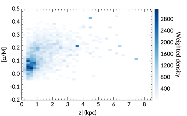
Figure 14: Variation of [$\alpha$/M] with distance from the Galactic plane for all stars. The density is weighted by selection bias fractions as described in Section 4. The over densities at high |z| are due to a few data points with large weights. Unlike metallicity, [$\alpha$/M] does not vary smoothly with increasing height. There appears to be a break in the distribution at |z| $\approx$ 1 kpc.

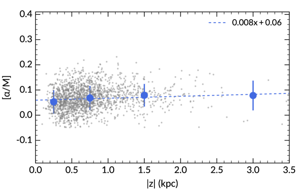
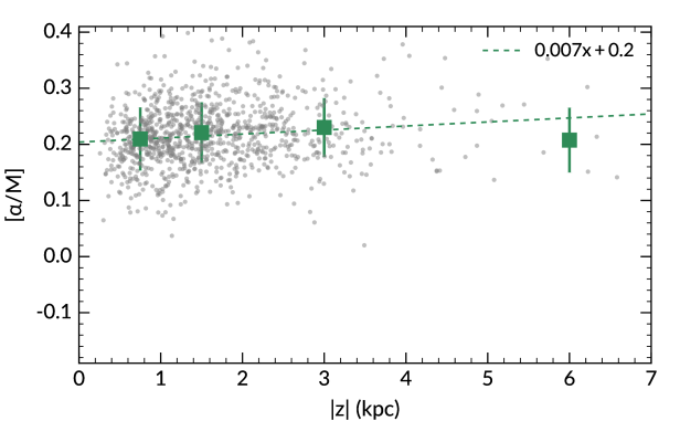
Figure 15: Variation of [$\alpha$/M] with distance from the Galactic plane for each of the high and low-$\alpha$ population. Top panel: vertical abundance gradient for the low-$\alpha$ stars. Bottom panel: vertical abundance gradient of the high-$\alpha$ stars. Both populations show a flat-positive trend. The high-$\alpha$ population shows a higher dispersion in [$\alpha$/M] values. The trends are fitted over grey data points, over-plotted are averaged values of four height bins and their one sigma error bars. Note that the binned values were not used in the gradient fitting.

Within the 1.5 kpc $R_{\textrm{GC}}$ range of our sample, we do not observe any significant radial changes in [$\alpha$/M] for either of the defined populations. Studies of the high-$\alpha$ population’s radial abundance gradients show that there is no variation, but there may be small positive radial [$\alpha$/M] gradients in the low-$\alpha$ population (e.g.,Mikolaitis et al. 2014; Bergemann et al. 2014). Genovali et al. (2015), however, found a negative radial abundance gradient for the $\alpha$-element Ca. Boeche et al. (2014) also found modest radial gradients for the $\alpha$-elements. The fact that we do not observe a radial abundance gradient in the low-$\alpha$ population is likely due to our limited radial coverage, which prevents us from assessing [$\alpha$/M] variation with $R_{\textrm{GC}}$.

The vertical $\alpha$-abundance profile of the entire sample is shown in Fig. 14, presented as a density plot similar to Fig. 12. The median [$\alpha$/M] increases as a function of height, as noted previously by Schlesinger et al. (2014) and Mikolaitis et al. (2014). However, unlike the metallicity, we find that the $\alpha$-abundance profile does not vary smoothly with $|z|$. The $\alpha$-abundance vertical gradient for the entire disk is d[$\alpha$/M]/d$z=0.038\pm 0.001$ dex kpc^-1. For the low and high-$\alpha$ populations, the [$\alpha$/M] vertical gradients are both slightly positive, as shown in Fig. 15. The gradients are d[$\alpha$/M]/d$z=0.008\pm 0.002$ dex kpc^-1 for the low-$\alpha$, and d[$\alpha$/M]/d$z=0.007\pm 0.002$ dex kpc^-1 for the high-$\alpha$ population. As in Section 5.3 above, we also analysed the two $\alpha$ populations with the ‘transition stars’ included. This did not change the slope measured for the low-$\alpha$ population, but increased the slope of the high-$\alpha$ population to d[$\alpha$/M]/d$z$ = $0.014\pm 0.001$ dex kpc^-1, which is higher than the value measured without transition stars. The transition stars contribute primarily at low $|z|$ ($\leq 1$ kpc), which is why their addition affected the high-$\alpha$ population more: as defined in Section 3.3, this population is mainly located at $|z|\geq 1$ kpc.

For the high-$\alpha$ population, Ruchti et al. (2011) showed that individual $\alpha$-abundances [Mg/Fe] and [Si/Fe] have vertical gradients $0.03\pm 0.02$ and $0.02\pm 0.01$ dex kpc^-1, respectively. Meanwhile, the vertical abundance gradients of [Ca/Fe] and [Ti i,ii/Fe] decrease to $-0.01\pm 0.01$ and $-0.02\pm 0.02$ dex kpc^-1. While we do not have $\alpha$-enhanced stars with [M/H] $<-1$ as in their study, this result is in agreement with the flat gradients we observe. Mikolaitis et al. (2014) also provide vertical gradients for the averaged [$\alpha$/M] abundances, as well as vertical gradients for individual $\alpha$-elements using $Gaia$-ESO iDR1. Mikolaitis et al. (2014) found similar vertical abundance profiles for the low and high-$\alpha$ stars. Both populations have averaged and individual vertical $\alpha$-abundance gradients of 0.04–0.05 dex kpc^-1, with errors $<0.01$ dex kpc^-1. These values are not in agreement with our measured vertical gradient for the $\alpha$ sub-populations, as we find that both populations have rather flat abundance distributions as a function of height. However, these results are similar to the gradient we derived for the disk overall. The differences could have arisen from the lack of correction for selection biases in Mikolaitis et al. (2014) and the different abundance scales of the $Gaia$-ESO and GALAH surveys. The [Mg/Fe] histograms shown in Fig. 3 of Mikolaitis et al. (2014) shows that $Gaia$-ESO iDR1 has a larger spread in their abundances compared to GALAH (c.f. Fig 5).

An important point to consider is the dependence of [$\alpha$/M] on [M/H], and the correlation of the latter with respect to vertical height |$z$|. At greater heights above the plane, observed stellar populations become more metal-poor (Fig 12), and these stars are typically more $\alpha$-enhanced. The positive $\alpha$-gradient over the entire disk is therefore reflective of the fact that more metal-poor, high-$\alpha$ stars become dominant at large heights. For each of the $\alpha$ sub-populations as defined in Fig 8, however, the correlation between [$\alpha$/M] and [M/H] is rather flat, which means that the small positive gradients we measured are intrinsic to these sub-populations.

Table 3: Summary of measured vertical gradients, and intercepts at |z| = 0 for disk metallicity and $\alpha$-abundances.

Population	d[M/H]/d$z$	$\sigma_{\textrm{d[M/H]/d}z}$	[M/H]($z=0$)	$\sigma_{\textrm{[M/H]($z=0$)}}$	d[$\alpha$/M]/d$z$	$\sigma_{\textrm{d[$\alpha$/M]/d}z}$	[$\alpha$/M]($z=0$)	$\sigma_{\textrm{[$\alpha$/M]($z=0$)}}$
	dex kpc-1		dex		dex kpc-1		dex
low-$\alpha$	$-0.18$	0.01	$-0.02$	0.01	+0.008	0.002	0.06	0.002
high-$\alpha$	$-0.058$	0.003	$-0.47$	0.01	+0.007	0.002	0.20	0.003
All stars	$-0.22$	0.01	$-0.08$	0.01	+0.038	0.001	0.08	0.002

7 Discussion

The process(es) that created the thick disk have been a central point of discussion in Galactic studies. The very definition of the thick disk has changed since first proposed by Gilmore & Reid (1983), and here we refer to the ‘thick disk’ as the overall more $\alpha$-enhanced population as defined in Section 3.3 using both chemical and kinematical information. In Section 1, we outlined the main scenarios that have been proposed for thick disk formation, and in this section we interpret our results in the context of these scenarios.

In summary, the vertical metallicity and abundance profiles of the disk show that:

(1) The disk overall has a steep negative vertical metallicity gradient.

(2) The low-$\alpha$ population has a similar vertical metallicity gradient to the full disk.

(3) The high-$\alpha$ population, on the other, has a much flatter vertical metallicity gradient.

(4) The $\alpha$-abundance ratio increases with height in general. At larger heights only the high-$\alpha$ population is present.

(5) Neither the high nor low-$\alpha$ sub-population show a significant vertical alpha abundance ratio gradient.

The vertical metallicity gradient in the high-$\alpha$ population is in contrast with predictions of the direct satellite accretion scenario proposed by Abadi et al. (2003) and the fast internal evolution model of Bournaud et al. (2009). While both of these scenarios could result in a chemically distinct thick disk, they also predict a uniform vertical metallicity distribution, or a lack of vertical metallicity gradient. Brook et al. (2004, 2005) proposed that the thick disk formed via merging of gas-rich clumps at high redshift, prior to the formation of the thin disk. Their model predicts an old, $\alpha$-enhanced thick disk that matches observations. However, their thick disk also shows no vertical metallicity gradient, in contrast to our results.

The heating of an existing disk by small satellite mergers can create a thick-disk like vertical structure (e.g., Quinn & Goodman 1986; Quinn et al. 1993; Kazantzidis et al. 2008; Villalobos & Helmi 2008). The vertical metallicity gradient of the existing disk could be preserved in the thick disk, however this can also be affected by the interplay between radial migration and radial metallicity gradients (e.g., Kawata et al. 2018). Bekki & Tsujimoto (2011) modelled the kinematics and chemistry of stars formed by minor mergers in detail, and showed that a fast star formation rate in the thick disk results in $\alpha$-enhanced stars. The steep vertical metallicity gradient of the pre-existing disk flattens over time, but qualitatively it is steeper in the inner Galaxy, consistent with the observations of Hayden et al. (2014). However, the final thick disk gradient is essentially flat at the solar circle, which is not what we observe. Furthermore, disk flaring is expected in such a heating scenario. For the high-$\alpha$ stars, Bovy et al. (2016) did not observe any flaring in their mono-abundance populations (MAPs). However, Minchev et al. (2015, 2016) argued that mono-age populations always flare in their cosmological simulations, and MAPs (mono-abundance populations) are not necessarily co-eval. Based on APOGEE abundances and calibrated ages, Mackereth et al. (2017) found that mono-age $\alpha$-enhanced populations do show some flaring, albeit with a smaller amplitude compared to the low-$\alpha$ population. Further observational and model constraints from stellar ages and flaring of the high-$\alpha$ stars are thus needed to understand the importance of minor mergers in thick disk formation.

The secular radial migration (Sellwood & Binney, 2002) process was proposed by Schönrich & Binney (2009) as the sole explanation for the thick disk (but this remains controversial, see e.g., Minchev & Famaey 2010; Vera-Ciro et al. 2014). Stars in the inner galaxy are formed fast and migrated outwards to create the $\alpha$-enhanced population at large scale heights. Since radial migration is more likely to affect older stars, a negative vertical metallicity gradient, and a positive [$\alpha$/M] gradient are expected. Schönrich & McMillan (2017) obtain d[M/H]/d$z\approx-0.2$ dex kpc^-1 for the full nearby disk in their analytical model (which included inside-out disk formation), in agreement with our observations. Loebman et al. (2011) also reported a similar vertical gradient of $\approx$$-0.18$ dex kpc^-1 in their N-body simulation with extensive radial migration. Both of these values are consistent with our measurements of the full disk and low-$\alpha$ population, even though Loebman et al. (2011) did not calibrate their model to reproduce the Milky Way.

Radial migration signatures are observed in the metallicity distribution function (MDF) of disk stars at different Galactocentric radii. Hayden et al. (2015) observed that at small heights above the plane, the skewness of MDFs changes from negative in the outer galaxy (skewed towards metal-poor stars) to positive (skewed towards metal rich stars) in the inner galaxy. In contrast, the high-$\alpha$ population’s MDF remain constant at all locations. Loebman et al. (2016) showed that these observations can be qualitatively explained by radial migration in their simulation. The change in skewness of the disk MDFs at different radii could be due to an increased fraction of migrated stars beyond $\approx$5 kpc, such that more metal rich stars are migrated to larger $R_{\textrm{GC}}$. As the high-$\alpha$ stars formed within a small region and a few Gyrs in a well mixed environment, their chemical content are similar and thus the MDF remains constant at all Galactic locations. Loebman et al. (2016) found a small vertical metallicity gradient in their simulated high-$\alpha$ population of $\approx$$-0.03$ dex kpc^-1. This is half the value observed in our study. Further investigation of the vertical metallicity and abundance gradients for the high-$\alpha$ stars in radial migration models will help to determine the extent to which it affects this population.

Bird et al. (2013) was able to produce a Milky Way-like galaxy with an old, vertically extended population much like the Galactic thick disk using the “Eris” cosmological simulation suite. The effects of the active merger phase at early times (redshift $>$ 3), secular heating, and radial migration on the present-day galaxy were examined. Bird et al. (2013) found that stars born during the merger phase have larger scale heights and shorter scale lengths, and younger populations form progressive thinner and longer structures. This gradual transition from a kinematically hot and thick disk to a colder, thinner disk was dubbed ‘upside down’ formation (see also Samland & Gerhard 2003). Interestingly, secular heating and radial migration did not have a large impact on the final properties of each coeval population. Rather, the trends are established at formation, suggesting that the thick disk-like component was born thick. Similarly, Stinson et al. (2013) and Brook et al. (2012) concluded that their $\alpha$-enhanced, older populations were born kinematically hot, and that the early disk settles into a thin component. The settling process of the galaxies and fast formation of the old, $\alpha$-enhanced and vertically extended populations in these simulations could produce the vertical metallicity and abundance profiles observed in this work. It was shown by Wisnioski et al. (2015) that the observed velocity dispersion of H$\alpha$ gas in galaxies at high redshift decreases with time, providing further indication that disk galaxies were born thick at redshifts of $z=1-2$.

While the cosmological models mentioned above heavily rely on the condition that disk galaxies like the Milky Way had a quiescent merger history, there is observational evidence that this may be true for the Galaxy (Ruchti et al., 2015; Casagrande et al., 2016). However, the metallicity and $\alpha$-abundance gradients in these simulations have not been studied in detail.

Although we observe an overall continuity in the vertical metallicity profile, we see two distinct $\alpha$-enhancement tracks as a function of $|z|$, which have implications for the star formation history of the disk. Haywood et al. (2013, 2016) proposed two different star formation epochs for the high and low-$\alpha$ stars. By comparing their chemical evolution model (Snaith et al., 2015) with APOGEE data, Haywood et al. (2016) proposed that the star formation rate dropped significantly at ages of 10 Gyr before increasing again at about 7 Gyr to a lower maximum value. This could indicate the transition between thick to thin disk formation. However, the authors note that due to the strict continuity of the stellar abundances, the gas supply must not have decreased during this period of time. Similarly, Brook et al. (2012) found that the star formation rate decreased slightly at around 7 Gyr, near the epoch of thin disk formation in their simulation. This idea was also explored by the two-infall model proposed by Chiappini et al. (1997), who argued for a decreased star formation rate between the epochs of halo-thick disk and thin disk formation, and proposed a shorter formation timescale for the halo/thick disk of 1 Gyr. Future work that incorporate stellar ages (e.g., from the GALAH/K2 overlap) will be able to rigorously test these scenarios and provide additional constraints on the formation time-scale of the thick disk.

8 Conclusion

We have determined the vertical profiles of metallicity and $\alpha$-abundances in the Galactic disk using data from the GALAH first internal data release. We analysed in total 3191 giants from the GALAH pilot and main surveys, extending up to 4 kpc in height above the plane, within a small range of Galactocentric distance ($7.9\la R_{\mathrm{GC}}\la 9.5$ kpc). The precise metallicity and abundance measurements of GALAH allow us to reliably define ‘thick’ and ‘thin’ disk populations using chemistry and radial velocities. The GALAH magnitude limits in the estimated $V$-band translate to a dependency in $(J-K)$ colour and magnitudes. We corrected for the selection effects for targets from the pilot and main surveys separately by population synthesis using BaSTI isochrones.

The vertical metallicity gradient of the entire disk is $-0.22\pm 0.01$ dex kpc^-1, which is in agreement with recent estimates from large spectroscopic surveys such as SEGUE and APOGEE. The low-$\alpha$ population, or the thin disk, also exhibits a steep negative vertical metallicity gradient d[M/H]/d$z=-0.18\pm 0.01$ dex kpc^-1. The more enhanced $\alpha$ population, which we identify as the thick disk, is found to have a shallower vertical gradient d[M/H]/d$z$ of $-0.058\pm 0.003$ dex kpc^-1. We note again that our data do not probe the metal-poor extension of the thick disk, however, the vertical gradients observed here are similar in amplitude to those of previous studies. Overall, our results confirm some conclusions reached by earlier studies, despite differences in target selection, spatial coverage and abundance scales. The discrepancies were likely caused by uncorrected selection effects in some cases, and the many different definitions in the literature of high-$\alpha$, or thick disk stars.

As expected, [$\alpha$/M] increases as a function of $|z|$, with the low-$\alpha$ population occupying lower heights on average. The vertical [$\alpha$/M] profile at the solar circle shows that there are two over-densities, with the discontinuity most clearly seen around $|z|=1$ kpc. We find that the both low and high-$\alpha$ sub-populations have a flat vertical [$\alpha$/M] gradient. Similarly, Ruchti et al. (2011) also found flat vertical gradients for individual $\alpha$-abundances at the metal-poor end of the $\alpha$-enhanced population. For the low-$\alpha$ population the gradient can be explained by radial migration playing an important role in the evolution of the thin disk. The negative vertical metallicity gradient in the high-$\alpha$ population indicate that scenarios which have uniform ‘thick disk’ vertical metallicity gradients are not responsible for its formation. The vertical [M/H] gradient observed in this work and elsewhere could have arisen from a settling phase of the disk as suggested by Samland & Gerhard (2003) and Bird et al. (2013), minor heating episodes such as in the models of Kazantzidis et al. (2008); Villalobos & Helmi (2008), or caused by radial migration (Schönrich & Binney, 2009; Loebman et al., 2011). Mergers cause flaring of the disk, which is seen in the low-$\alpha$ population in the analysis of Bovy et al. (2016), but not in the high-$\alpha$ population. However, Mackereth et al. (2017) have since shown that coeval high-$\alpha$ populations do indeed show flaring, but much less than the low-$\alpha$ stars. On the other hand, the $\alpha$-abundances of both sub-populations are distinct and nearly constant at all heights, indicating that they are formed in very different conditions.

Accurate distances and proper motion from Gaia DR2 will allow for an even more accurate and detailed analysis of the chemistry and kinematics of the high-$\alpha$ population, not only for the GALAH pilot survey but also the larger GALAH main sample. This will give us a clearer and more definitive picture of the formation and evolution of the Milky Way thick disk.

Appendix A Online data table

Table 4: An example of the contents included in the online data table. The complete table is available on the publisher website.

OBJECT ID	UCAC4 ID	RAJ2000	DEJ2000	Distance	Pr(thick)
		deg	deg	pc
131216002101010	156-011705	115.5245	-58.9095	1102.72	0.1583
131216002101012	156-011845	116.1019	-58.9680	1502.33	0.0009
131216002101013	156-011859	116.1602	-58.9823	3058.82	0.0188
131216002101018	156-011814	115.9660	-58.9922	854.35	0.0083
131216002101021	155-011860	116.3630	-59.0953	2287.51	0.0180
131216002101023	155-011759	116.0724	-59.0578	2200.28	0.0096
131216002101025	155-011806	116.2236	-59.1011	2078.00	0.2680
131216002101028	156-011737	115.6524	-58.9935	628.69	0.0003
131216002101029	155-011714	115.9342	-59.0706	1578.78	0.0079
131216002101033	155-011844	116.3374	-59.1984	871.58	0.0021

We have included a data table listing the stars analysed in this work, their GALAH object ID, UCAC4 catalogue ID, coordinates, thick disk membership probability and distances. Table 4 provides an example of the contents included in the online material.

References

- Abadi et al. (2003) Abadi M. G., Navarro J. F., Steinmetz M., Eke V. R., 2003, ApJ, 591, 499
- Adibekyan et al. (2011) Adibekyan V. Z., Santos N. C., Sousa S. G., Israelian G., 2011, A&A, 535, L11
- Adibekyan et al. (2013) Adibekyan V. Z., et al., 2013, A&A, 554, A44
- Amarsi et al. (2015) Amarsi A. M., Asplund M., Collet R., Leenaarts J., 2015, MNRAS, 454, L11
- Amarsi et al. (2016) Amarsi A. M., Asplund M., Collet R., Leenaarts J., 2016, MNRAS, 455, 3735
- Anguiano et al. (2015) Anguiano B., et al., 2015, MNRAS, 451, 1229
- Astraatmadja & Bailer-Jones (2016) Astraatmadja T. L., Bailer-Jones C. A. L., 2016, ApJ, 833, 119
- Aumer et al. (2016) Aumer M., Binney J., Schönrich R., 2016, MNRAS, 459, 3326
- Bartašiūtė et al. (2003) Bartašiūtė S., Aslan Z., Boyle R. P., Kharchenko N. V., Ossipkov L. P., Sperauskas J., 2003, BaltA, 12, 539
- Bekki & Tsujimoto (2011) Bekki K., Tsujimoto T., 2011, ApJ, 738, 4
- Bensby et al. (2011) Bensby T., Alves-Brito A., Oey M. S., Yong D., Meléndez J., 2011, ApJ, 735, L46
- Bensby et al. (2014) Bensby T., Feltzing S., Oey M. S., 2014, A&A, 562, A71
- Bergemann et al. (2014) Bergemann M., et al., 2014, A&A, 565, A89
- Bird et al. (2013) Bird J. C., Kazantzidis S., Weinberg D. H., Guedes J., Callegari S., Mayer L., Madau P., 2013, ApJ, 773, 43
- Bland-Hawthorn & Gerhard (2016) Bland-Hawthorn J., Gerhard O., 2016, ARA&A, 54, 529
- Boeche et al. (2014) Boeche C., et al., 2014, A&A, p. A71
- Bournaud et al. (2009) Bournaud F., Elmegreen B. G., Martig M., 2009, ApJ, 707, L1
- Bovy et al. (2012a) Bovy J., Rix H.-W., Hogg D. W., 2012a, ApJ, 751, 131
- Bovy et al. (2012b) Bovy J., Rix H.-W., Liu C., Hogg D. W., Beers T. C., Lee Y. S., 2012b, ApJ, 753, 148
- Bovy et al. (2016) Bovy J., Rix H.-W., Schlafly E. F., Nidever D. L., Holtzman J. A., Shetrone M., Beers T. C., 2016, ApJ, 823, 30
- Brook et al. (2004) Brook C. B., Kawata D., Gibson B. K., Freeman K. C., 2004, ApJ, 612, 894
- Brook et al. (2005) Brook C. B., Gibson B. K., Martel H., Kawata D., 2005, ApJ, 630, 298
- Brook et al. (2012) Brook C. B., et al., 2012, MNRAS, 426, 690
- Brown et al. (2016) Brown A. G. A., et al., 2016, A&A, 595, A2
- Burkert et al. (1992) Burkert A., Truran J. W., Hensler G., 1992, ApJ, 391, 651
- Burnett & Binney (2010) Burnett B., Binney J., 2010, MNRAS, 407, 339
- Burstein (1979) Burstein D., 1979, ApJ, 234, 829
- Casagrande et al. (2010) Casagrande L., Ramírez I., Meléndez J., Bessell M., Asplund M., 2010, A&A, 512, 54
- Casagrande et al. (2011) Casagrande L., Schönrich R., Asplund M., Cassisi S., Ramírez I., Meléndez J., Bensby T., Feltzing S., 2011, A&A, 530, A138
- Casagrande et al. (2014) Casagrande L., Aguirre V. S., Stello D., Huber D., Serenelli A. M., Cassisi S., Dotter A., 2014, ApJ, 787, 110
- Casagrande et al. (2016) Casagrande L., et al., 2016, MNRAS, 455, 987
- Chen et al. (2011) Chen Y. Q., Zhao G., Carrell K., Zhao J. K., 2011, AJ, 142, 184
- Cheng et al. (2012) Cheng J. Y., et al., 2012, ApJ, 752, 51
- Chiappini et al. (1997) Chiappini C., Matteucci F., Gratton R., 1997, ApJ, 477, 765
- Chiba & Beers (2000) Chiba M., Beers T. C., 2000, AJ, 119, 2843
- Ciucǎ et al. (2018) Ciucǎ I., Kawata D., Lin J., Casagrande L., Seabroke G., Cropper M., 2018, MNRAS, 475, 1203
- Comerón et al. (2015) Comerón S., Salo H., Janz J., Laurikainen E., Yoachim P., 2015, A&A, 584, A43
- Dalcanton & Bernstein (2002) Dalcanton J. J., Bernstein R. A., 2002, AJ, 124, 1328
- Dalton et al. (2016) Dalton G., et al., 2016, Proc. SPIE: Ground-based and Airborne Instrumentation for Astronomy VI, 9908, 99081G
- De Silva et al. (2015) De Silva G. M., et al., 2015, MNRAS, 449, 2604
- Dempster et al. (1977) Dempster A. P., Laird N. M., Rubin D. B., 1977, J. R. Stat. Soc. B, 39, 1
- Dierickx et al. (2010) Dierickx M., Klement R., Rix H.-W., Liu C., 2010, ApJ, 725, L186
- Drimmel & Spergel (2001) Drimmel R., Spergel D. N., 2001, ApJ, 556, 181
- Edvardsson et al. (1993) Edvardsson B., Andersen J., Gustafsson B., Lambert D. L., Nissen P. E., Tomkin J., 1993, A&A, 275, 101
- Forbes et al. (2012) Forbes J., Krumholz M., Burkert A., 2012, ApJ, 754, 48
- Fuhrmann (2008) Fuhrmann K., 2008, MNRAS, 384, 173
- Furhmann et al. (2016) Furhmann K., Chini R., Kaderhandt L., Chen Z., 2016, MNRAS, 464, 2610
- Genovali et al. (2014) Genovali K., et al., 2014, A&A, 566, A37
- Genovali et al. (2015) Genovali K., et al., 2015, A&A, 580, A17
- Gilmore & Reid (1983) Gilmore G., Reid N., 1983, MNRAS, 202, 1025
- Gilmore et al. (1995) Gilmore G., Wyse R. F. G., Jones J. B., 1995, AJ, 109, 1095
- Gilmore et al. (2002) Gilmore G., Wyse R. F. G., Norris J. E., 2002, ApJ, 574, L39
- Gilmore et al. (2012) Gilmore G., et al., 2012, The Messenger, 147, 25
- Gratton et al. (2000) Gratton R. G., Carretta E., Matteucci F., Sneden C., 2000, A&A, 358, 671
- Grevesse et al. (2007) Grevesse N., Asplund M., Sauval A. J., 2007, Space Sci. Rev., 130, 105
- Gustafsson et al. (2008) Gustafsson B., Edvardsson B., Eriksson K., Jorgensen U. G., Nordlund A., Plez B., 2008, A&A, 486, 951
- Hayden et al. (2014) Hayden M. R., et al., 2014, AJ, 147, 116
- Hayden et al. (2015) Hayden M. R., et al., 2015, ApJ, 808, 132
- Haywood (2008) Haywood M., 2008, MNRAS, 388, 1175
- Haywood et al. (2013) Haywood M., Di Matteo P., Lehnert M. D., Katz D., Gómez A., 2013, A&A, 560, A109
- Haywood et al. (2015) Haywood M., Di Matteo P., Snaith O., Lehnert M. D., 2015, A&A, 579, A5
- Haywood et al. (2016) Haywood M., Lehnert M. D., Di Matteo P., Snaith O., Schultheis M., Katz D., Gomez A., 2016, A&A, 589, 17
- Heiter et al. (2015) Heiter U., Jofré P., Gustafsson B., Korn A. J., Soubiran C., Thévenin F., 2015, A&A, 582, A49
- Huber et al. (2017) Huber D., et al., 2017, ApJ, 844, 102
- Ibata et al. (2009) Ibata R., Mouhcine M., Rejkuba M., 2009, MNRAS, 395, 126
- Jofré et al. (2014) Jofré P., et al., 2014, A&A, 564, A133
- Jurić et al. (2008) Jurić M., et al., 2008, ApJ, 673, 864
- Katz et al. (2011) Katz D., Soubiran C., Cayrel R., Barbuy B., Friel E., Bienaymé O., Perrin M., 2011, A&A, 525, A90
- Kawata et al. (2017) Kawata D., Grand R. J. J., Gibson B. K., Casagrande L., Hunt J. A. S., Brook C. B., 2017, MNRAS, 464, 702
- Kawata et al. (2018) Kawata D., et al., 2018, MNRAS, 473, 867
- Kazantzidis et al. (2008) Kazantzidis S., Bullock J. S., Zentner A. R., Kravtsov A. V., Moustakas L. A., 2008, ApJ, 688, 254
- Kordopatis et al. (2011) Kordopatis G., et al., 2011, A&A, 535, A107
- Kordopatis et al. (2017) Kordopatis G., Wyse R. F., Chiappini C., Minchev I., Anders F., Santiago B., 2017, MNRAS, 467, 469
- Kos et al. (2017) Kos J., et al., 2017, MNRAS, 464, 1259
- Lind et al. (2012) Lind K., Bergemann M., Asplund M., 2012, MNRAS, 427, 27
- Loebman et al. (2011) Loebman S. R., Roškar R., Debattista V. P., Ivezić Ž., Quinn T. R., Wadsley J., 2011, ApJ, 737, 8
- Loebman et al. (2016) Loebman S. R., Debattista V. P., Nidever D. L., Hayden M. R., Holtzman J. A., Clarke A. J., Ro R., Valluri M., 2016, ApJ, 818, L6
- Mackereth et al. (2017) Mackereth J. T., et al., 2017, MNRAS, 471, 3057
- Majewski et al. (2011) Majewski S. R., Zasowski G., Nidever D. L., 2011, ApJ, 739, 25
- Majewski et al. (2015) Majewski S. R., et al., 2015, preprint (arXiv:1509.05420)
- Marigo et al. (2017) Marigo P., et al., 2017, ApJ, 835, 77
- Marsakov & Borkova (2006) Marsakov V. A., Borkova T. V., 2006, AstL, 32, 376
- Martell et al. (2017) Martell S. L., et al., 2017, MNRAS, 465, 3203
- Martig et al. (2016a) Martig M., et al., 2016a, MNRAS, 456, 3655
- Martig et al. (2016b) Martig M., Minchev I., Ness M., Fouesneau M., Rix H.-W., 2016b, ApJ, 831, 139
- Mashonkina et al. (2003) Mashonkina L., Gehren T., Travaglio C., Borkova T., 2003, A&A, 397, 275
- Matteucci & François (1989) Matteucci F., François P., 1989, MNRAS, 239, 885
- Michalik et al. (2015) Michalik D., Lindegren L., Hobbs D., 2015, A&A, 574, A115
- Mikolaitis et al. (2014) Mikolaitis Š., et al., 2014, A&A, 572, A33
- Minchev & Famaey (2010) Minchev I., Famaey B., 2010, ApJ, 722, 112
- Minchev et al. (2015) Minchev I., Martig M., Streich D., Scannapieco C., de Jong R. S., Steinmetz M., 2015, ApJ, 804, L9
- Minchev et al. (2016) Minchev I., Steinmetz M., Chiappini C., Martig M., Anders F., Matijevic G., Jong R. S. D., 2016, ApJ, 834, 27
- Nemec & Nemec (1993) Nemec J. M., Nemec A. F. L., 1993, AJ, 105, 1455
- Ness et al. (2015) Ness M., Hogg D. W., Rix H.-W., Ho A. Y. Q., Zasowski G., 2015, ApJ, 808, 16
- Nissen & Schuster (2010) Nissen P. E., Schuster W. J., 2010, A&A, 511, L10
- Norris (1987) Norris J., 1987, ApJ, 314, L39
- Ojha (2001) Ojha D. K., 2001, MNRAS, 322, 426
- Pedregosa et al. (2011) Pedregosa F., et al., 2011, JMLR, 12, 2825
- Pietrinferni et al. (2004) Pietrinferni A., Santi C., Salaris M., Castelli F., 2004, ApJ, 612, 168
- Piskunov & Valenti (2017) Piskunov N., Valenti J. A., 2017, A&A, 597, A16
- Prieto et al. (2006) Prieto C. A., Beers T. C., Wilhelm R., Newberg H. J., Rockosi C. M., Yanny B., Lee Y. S., 2006, ApJ, 636, 804
- Prochaska et al. (2000) Prochaska J. X., et al., 2000, AJ, 120, 2513
- Quinn & Goodman (1986) Quinn P. J., Goodman J., 1986, ApJ, 309, 472
- Quinn et al. (1993) Quinn P. J., Hernquist L., Fullagar D. P., 1993, ApJ, 403, 74
- Rahimi et al. (2014) Rahimi A., Carrell K., Kawata D., 2014, RAA, 14, 1406
- Recio-Blanco et al. (2014) Recio-Blanco A., et al., 2014, A&A, 567, A5
- Robin et al. (2003) Robin A. C., Reylé C., Derrière S., Picaud S., 2003, A&A, 409, 523
- Rojas-Arriagada et al. (2016) Rojas-Arriagada A., et al., 2016, A&A, 586, A39
- Roškar et al. (2012) Roškar R., Debattista V. P., Quinn T. R., Wadsley J., Lancashire C., Pr P., 2012, MNRAS, 426, 2089
- Ruchti et al. (2011) Ruchti G. R., et al., 2011, ApJ, 737, 9
- Ruchti et al. (2015) Ruchti G. R., et al., 2015, MNRAS, 450, 2874
- Sales et al. (2009) Sales L. V., et al., 2009, MNRAS, 400, L61
- Salpeter (1955) Salpeter E. E., 1955, ApJ, 121, 161
- Samland & Gerhard (2003) Samland M., Gerhard O. E., 2003, A&A, 399, 961
- Schlegel et al. (1998) Schlegel D. J., Finkbeiner D. P., Davis M., 1998, ApJ, 500, 525
- Schlesinger et al. (2014) Schlesinger K. J., et al., 2014, ApJ, 791, 112
- Schönrich & Binney (2009) Schönrich R., Binney J., 2009, MNRAS, 399, 1145
- Schönrich & McMillan (2017) Schönrich R., McMillan P. J., 2017, MNRAS, 18, 1154
- Sellwood & Binney (2002) Sellwood J. A., Binney J., 2002, MNRAS, 336, 785
- Sharma et al. (2011) Sharma S., Bland-Hawthorn J., Johnston K. V., Binney J., 2011, ApJ, 730, 3
- Sharma et al. (2018) Sharma S., et al., 2018, MNRAS, 473, 2004
- Skrutskie et al. (2006) Skrutskie M. F., et al., 2006, AJ, 131, 1163
- Snaith et al. (2015) Snaith O., Haywood M., Matteo P. D., Lehnert M. D., Combes F., Katz D., Gómez A., 2015, A&A, 578, A87
- Stassun & Torres (2016) Stassun K. G., Torres G., 2016, ApJ, 831, L6
- Steinmetz et al. (2006) Steinmetz M., et al., 2006, AJ, 132, 1645
- Stello et al. (2017) Stello D., et al., 2017, ApJ, 835, 83
- Stinson et al. (2013) Stinson G. S., et al., 2013, MNRAS, 436, 625
- Stonkutė et al. (2016) Stonkutė E., et al., 2016, MNRAS, 460, 1131
- Ting et al. (2015) Ting Y.-S., Conroy C., Goodman A., 2015, ApJ, 807, 104
- Tsikoudi (1979) Tsikoudi V., 1979, ApJ, 234, 842
- Valenti & Piskunov (1996) Valenti J. A., Piskunov N., 1996, A&AS, 118, 595
- Vera-Ciro et al. (2014) Vera-Ciro C., D’Onghia E., Navarro J., Abadi M., 2014, ApJ, 794, 173
- Villalobos & Helmi (2008) Villalobos Á., Helmi A., 2008, MNRAS, 391, 1806
- Wisnioski et al. (2015) Wisnioski E., et al., 2015, ApJ, 209, 799
- Wright et al. (2010) Wright E. L., et al., 2010, AJ, 140, 1868
- Wyse & Gilmore (1988) Wyse R. F. G., Gilmore G., 1988, AJ, 95, 1404
- Wyse et al. (2006) Wyse R. F. G., Gilmore G., Norris J. E., Wilkinson M. I., Kleyna J. T., Koch A., Evans N. W., Grebel E. K., 2006, ApJ, 639, L13
- Yoachim & Dalcanton (2006) Yoachim P., Dalcanton J. J., 2006, AJ, 131, 226
- Yoshii (1982) Yoshii Y., 1982, PASJ, 34, 365
- Zasowski et al. (2013) Zasowski G., et al., 2013, AJ, 146, 81
- Zwitter et al. (2010) Zwitter T., et al., 2010, A&A, 522, A54
- de Jong et al. (2011) de Jong R. D., et al., 2011, The Messenger, 145, 14