Towards a quantum time mirror for nonrelativistic wave packets

Abstract

We propose a method – a quantum time mirror (QTM) – for simulating a partial time-reversal of the free-space motion of a nonrelativistic quantum wave packet. The method is based on a short-time spatially-homogeneous perturbation to the wave packet dynamics, achieved by adding a nonlinear time-dependent term to the underlying Schrödinger equation. Numerical calculations, supporting our analytical considerations, demonstrate the effectiveness of the proposed QTM for generating a time-reversed echo image of initially localized matter-wave packets in one and two spatial dimensions. We also discuss possible experimental realizations of the proposed QTM.

I Introduction

The question of how to invert the time evolution of a wave, classical or quantum, in an efficient and controllable way has both fundamental and practical importance. The fundamental aspect of the question is evident from its connection with the problem of unidirectionality of the arrow of time, conceived in a seminal 19th century debate between Loschmidt and Boltzmann Loschmidt (1876); Boltzmann (1877). The practical importance is apparent from numerous applications in medicine, telecommunication, material analysis, and, more generally, wave control Fink (1997, 1999); Lerosey et al. (2007); Mosk et al. (2012); Bacot et al. (2016).

One fruitful approach to the time inversion of classical wave motion is based on the concept of a time-reversal mirror: an array of receiver-emitter antennas is used to first record an incident wavefront, originating say from a localized source, and then to rebroadcast a time-inverted copy of the recording, thus generating a wave that effectively propagates backward in time and refocuses at the source point. To date, time reversal mirrors have been successfully implemented with acoustic Fink (1992); Draeger and Fink (1997), elastic Fink (1997), electromagnetic Lerosey et al. (2004), and water waves Przadka et al. (2012); Chabchoub and Fink (2014).

The classical procedure at the heart of such time-reversal mirrors, i.e. a continuous measurement and a subsequent reinjection of the signal, cannot be directly applied to quantum systems. The fundamental obstacle here is that any measurement performed on a quantum system is bound to perturb the quantum state and consequently affects its time evolution. (A theoretical scenario in which a time-dependent wave function is measured, recorded and then “played back” by a perfect non-invasive detector-emitter has been analyzed in Refs. Pastawski et al. (2007); Calvo and Pastawski (2010)) An alternative approach to manipulate the propagation of waves relies on non-adiabatic perturbations to the system dynamics, such as an instantaneous change of its boundary conditions Moshinsky (1952); Gerasimov and Kazarnovskii (1976); Č. Brukner and Zeilinger (1997); Mendonça and Shukla (2002); del Campo et al. (2009); Goussev (2012); Haslinger et al. (2013); Goussev (2013). Protocols of this kind were considered for time- and space-modulated one-dimensional photonic Sivan and Pendry (2011a, b, c) and magnonic crystals Chumak et al. (2010); Karenowska et al. (2012). More recently, Bacot et al.  put forward and experimentally realized an instantaneous time mirror for gravity-capillary waves, requiring a sudden but homogenous modulation of water wave celerity Bacot et al. (2016). Such approaches bypass the recording procedure, and are thus very appealing for quantum systems. A specific time-reversal protocol, albeit valid in a very narrow momentum range, was indeed devised for a one-dimensional periodically-kicked optical lattice Martin et al. (2008) and realized in a ⁸⁷Rb Bose-Einstein condensate (BEC) Ullah and Hoogerland (2011). On the other hand, an instantaneous quantum time mirror (QTM) for Dirac-like systems (exploiting their spinor structure) was recently proposed in Ref. Reck et al. (2017).

In this paper, we propose and investigate an experimentally realizable method for simulating the time-reversal of the free-space motion, thus mimicking a nonlinear QTM, for a spatially extended (orbital) quantum-mechanical wave function, such as a BEC cloud. The approach relies on generating a short-time spatially-uniform perturbation to the wave packet dynamics that corresponds to an additional nonlinear term added in the Schrödinger equation; in a BEC cloud system, such a perturbation can be realized using established experimental techniques allowing to tune the strength of the interaction among the cloud atoms Inouye et al. (1998); Roberts et al. (1998). More precisely, our QTM protocol comprises three stages: (i) a matter-wave packet propagates freely in space for a time $0<t<t_{0}$; (ii) at $t=t_{0}$, a strong nonlinear perturbation is switched on globally for a short period $\delta t$, leading to a near-instantaneous modification of the position-dependent phase of the wave function; (iii) the perturbation is switched off, the wave function evolves freely again, and at a time $t_{\rm echo}>t_{0}+\delta t$ an “echo” signal of the original wave packet is observed. From the conceptual viewpoint, the nonlinear QTM proposed in this paper can be viewed as a quantum-mechanical counterpart of the instantaneous time mirror for gravity-capillary waves by Bacot et al. Bacot et al. (2016).

The paper is organized as follows. In Sec. II, we describe the physical principle underling the proposed QTM. Two concrete scenarios for generating a time-reversed motion of matter waves in one and two spatial dimensions are analyzed in Sec. III. A summary, concluding remarks, and a discussion of the feasibility of an experimental realization of the proposed QTM are presented in Sec. IV. Technical calculations are deferred to an appendix.

II Physical principle of a nonlinear quantum time mirror

We address the time evolution of a matter-wave packet $\Psi({\bf r},t)$, subject to the initial condition $\Psi({\bf r},0)=\Psi_{0}({\bf r})$, in accordance with the $(D+1)$-dimensional nonlinear Schrödinger equation

$$i\hbar\frac{\partial\Psi}{\partial t}=-\frac{\hbar^{2}}{2m}\nabla^{2}\Psi+\lambda f(t-t_{0})|\Psi|^{2}\Psi.$$ (1)

Here, $m$ is the atomic mass, $\lambda$ quantifies the nonlinearity strength, and $t_{0}$ denotes the time around which the nonlinear term representing interaction effects is switched on. The function $f(\zeta)$ is sharply peaked around $\zeta\!=\!0$ and is chosen to satisfy the normalization condition $\int_{-\infty}^{+\infty}\,{\rm d}\zeta f(\zeta)=1$. We take $f$ to be a $\delta$-function in our analytical calculations and a Gaussian peak $f(\zeta)=\frac{1}{\sqrt{2\pi}\Delta t}e^{-\frac{\zeta^{2}}{2\Delta t^{2}}}$ in all numerical simulations. The pulse length $\Delta t\ll t_{0}$ will be taken as $0.001t_{0}$ and $0.0025t_{0}$ in one and two dimensions, respectively.

Wave packet dynamics in the presence of an infinitesimally short nonlinear kick, $f(\zeta)\!=\!\delta(\zeta)$, can be described as follows. Rescaling $t\rightarrow t_{0}t$, ${\bf r}\rightarrow\sqrt{\frac{\hbar t_{0}}{m}}{\bf r}$, $\Psi\rightarrow\left(\frac{m}{\hbar t_{0}}\right)^{D/4}\Psi$, and $\lambda\rightarrow\hbar\left(\frac{\hbar t_{0}}{m}\right)^{D/2}\lambda$, we write the nonlinear Schrödinger equation in a dimensionless form as

$$i\frac{\partial\Psi}{\partial t}=-\frac{1}{2}\nabla^{2}\Psi+\lambda\delta(t-1)|\Psi|^{2}\Psi\,.$$ (2)

The evolution of the wave function from $\Psi_{0}({\bf r})$ at $t=0$ to its value $\Psi_{-}({\bf r})=\Psi({\bf r},t=1^{-})$ right before the kick is given by

$$\Psi_{-}({\bf r})=\int\,{\rm d}^{D}{\bf r}^{\prime}K({\bf r}-{\bf r}^{\prime},t)\Psi_{0}({\bf r}^{\prime})\,,$$ (3)

where the integration runs over the infinite $D$-dimensional space, and $K({\bf q},t)\!=\!(2\pi it)^{-D/2}\exp{[i|{\bf q}|^{2}/(2t)]}$ is the free-particle propagator. The nonlinear kick results in an instantaneous change of the wave function from $\Psi_{-}({\bf r})$ at $t=1^{-}$ to

$$\Psi_{+}({\bf r})=\Psi_{-}({\bf r})e^{-i\lambda|\Psi_{-}({\bf r})|^{2}}$$ (4)

at $t=1^{+}$. Indeed, during the time interval $1^{-}<t<1^{+}$, the wave function transformation is dominated by the second term in the right-hand side of Eq. (2), and effectively governed by the differential equation $\frac{\partial\ln\Psi({\bf r},t)}{\partial t}=-i\lambda|\Psi_{-}({\bf r})|^{2}\delta(t-1)$, the solution of which is given by Eq. (4). After the kick, the wave function evolves freely, so that $\Psi({\bf r},t)=\int\,{\rm d}^{D}{\bf r}^{\prime}K({\bf r}-{\bf r}^{\prime},t)\Psi_{+}({\bf r}^{\prime})$ for all times $t>1$.

As evident from Eq. (4), the instantaneous nonlinear kick alters the phase of the wave function without producing any probability density redistribution, so that $\rho({\bf r})\equiv|\Psi_{+}({\bf r})|^{2}=|\Psi_{-}({\bf r})|^{2}$. The phase change however affects the probability current, whose dimensionless expression reads ${\bf j}({\bf r},t)=\mathrm{Im}\big{[}\Psi^{*}({\bf r},t)\nabla\Psi({\bf r},t)\big{]}$. A straightforward evaluation of the current right after the kick, ${\bf j}_{+}=\mathrm{Im}\big{[}\Psi_{+}^{*}\nabla\Psi_{+}\big{]}$, yields

$${\bf j}_{+}={\bf j}_{-}+\Delta{\bf j}\qquad\mathrm{with}\qquad\Delta{\bf j}=-\lambda\rho\nabla\rho\,,$$ (5)

where ${\bf j}_{-}=\mathrm{Im}\big{[}\Psi_{-}^{*}\nabla\Psi_{-}\big{]}$ is the probability current immediately preceding the kick. This in turn means that, by properly tuning the kicking strength $\lambda$, the wave propagation direction can be reversed for those parts of the matter wave for which the vector $\nabla\rho$ is aligned (or anti-aligned) with ${\bf j}_{-}$. Below we show that in geometries accessible in atom-optics experiments this reversal effect is robust and well-pronounced.

III The quantum time mirror at work

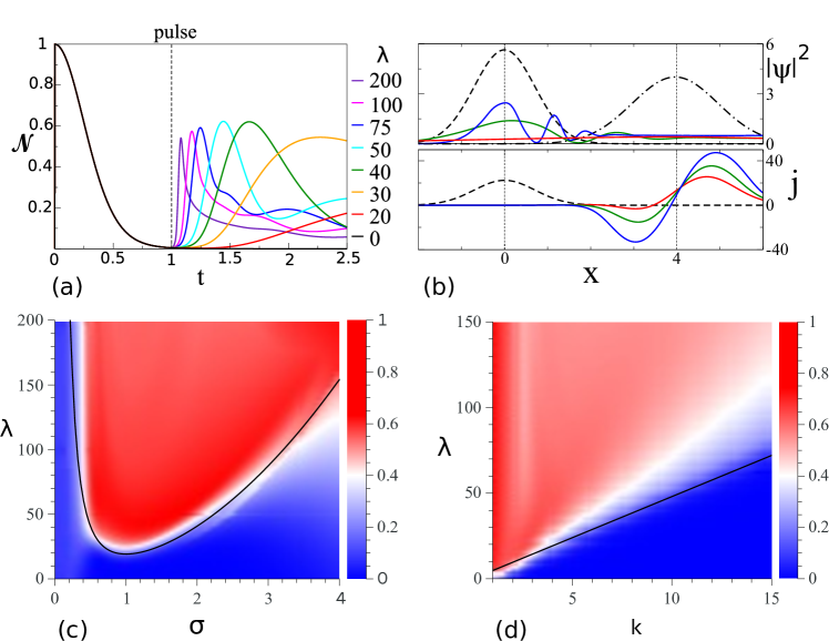
Figure 1: Echo of a 1D Gaussian wave packet subjected to a short, nonlinear pulse. All quantities are dimensionless according to the rescaling in the text above Eq. (2). (a) Norm correlation, Eq. (9), as a function of time for various pulse strengths $\lambda$ of a kick at $t=1$ at fixed wave packet width $\sigma=1$ and momentum $k=4$, yielding echoes up to $60\%$. (b) Upper panel: real space probability density $\rho=|\psi|^{2}$ at $t=0$ (black dashed curve), $t=0.99$ (just before pulse, black dashed-dotted curve), and at the peak echo times (colored curves, color code as in (a)). Notice that the latter depend on $\lambda$, as evident from (a). Lower panel: current density $j$ at $t=0$ (black dashed curve) and $t=1.01$ (right after the pulse, color code as in (a)). A negative current density indicates the part of the wave packet reversing its propagation direction thereby causing the echo. The minimal kicking strength for the used parameters, as predicted by Eq. (7), is $\lambda_{\min}\simeq 20$ (red curve); the associated negative current density is not sufficient for echo generation. Panels (c) and (d) show the echo strength, i.e. the maximal achieved value of the norm correlation after the pulse for a given parameter set. The parameter, which is kept constant is (c) $k=4$, (d) $\sigma=1$. The black curves are the analytical approximations (Eq. (7) for the minimal pulse strength $\lambda_{\min}$ required to generate an echo and matches well the numerical results.

As our first example, we consider the case of the initial state given by a 1D Gaussian wave packet,

$$\Psi_{0}(x)=(\pi\sigma^{2})^{-1/4}\exp\left(-\frac{x^{2}}{2\sigma^{2}}+ikx\right),$$ (6)

characterized by the dimensionless real spatial dispersion $\sigma$ and average momentum $k$. The corresponding wave function at time $t=1^{-}$ is obtained from Eq. (3) and reads (up to a position-independent phase factor) $\Psi_{-}(x)=[\pi(\sigma^{2}+\sigma^{-2})]^{-1/4}\exp[-\xi^{2}/2(\sigma^{2}+i)+ik\xi]$ with $\xi=x-k$ denoting the distance from the wave packet center. Thus, the probability density at $t=1$ is $\rho=\exp(-\xi^{2}/\sigma_{1}^{2})/\sqrt{\pi}\sigma_{1}$, where $\sigma_{1}=\sqrt{\sigma^{2}+\sigma^{-2}}$ is the dispersion of the wave packet at the time of the kick. The probability currents before and after the kick are, respectively, $j_{-}=\left(k+\frac{\xi}{\sigma^{2}\sigma_{1}^{2}}\right)\rho$ and $j_{+}=j_{-}+\Delta j$, with $\Delta j=\frac{2\lambda\xi}{\sigma_{1}^{2}}\rho^{2}$. The minimal kick strength $\lambda_{\min}$ necessary for reversing the direction of motion of (and effectively reflecting) a part of the wave packet can be estimated by requiring $j_{+}=0$ at $\xi=-\sigma_{1}$. In the case of a fast moving wave packet, such that $k\gg 1/\sigma^{2}\sigma_{1}$, this estimation yields

$$\lambda_{\min}\simeq Ck\left(\sigma^{2}+\frac{1}{\sigma^{2}}\right)$$ (7)

with $C=e\sqrt{\pi}/2\simeq 2.4$. Then, given a kicking strength $\lambda>\lambda_{\min}$, the time $t_{\mathrm{echo}}$ at which the reflected part of the wave packet reaches its initial position, leading to a partial echo of the original wave packet, can be evaluated as follows. The velocity of the reflected wave is $k_{\mathrm{rev}}\simeq j_{+}\big{|}_{\xi=-\sigma_{1}}\simeq k-\frac{\lambda}{C\sigma_{1}^{2}}=\left(1-\frac{\lambda}{\lambda_{\min}}\right)k$, and the revival occurs when $|k_{\mathrm{rev}}|(t_{\text{echo}}-1)=k$ or, correspondingly, at

$$t_{\text{echo}}=\frac{\lambda}{\lambda-\lambda_{\min}}\,.$$ (8)

The numerical simulations are based on the wave packet propagation algorithm Time-dependent Quantum Transport (TQT) Krückl (2013). The state is discretized on a square grid and the time evolution is calculated for sufficiently small time steps such that the Hamilton operator can be assumed time independent for each step. We calculate the action of $H$ on $\psi$ in a mixed position and momentum-space representation by the application of Fourier Transforms. With this a Krylov Space is spanned, which can be used to calculate the time evolution using a Lanczos method Lanczos (1950).

The echo strength is quantified by the norm correlation between the initial and the time propagated wave packet defined as Eckhardt (2003)

$$\mathcal{N}(t)=\frac{\int\,{\rm d}^{D}{\bf r}\left|\Psi_{0}({\bf r})\right|^{2}\left|\Psi({\bf r},t)\right|^{2}}{\sqrt{\int\,{\rm d}^{D}{\bf r}\left|\Psi_{0}({\bf r})\right|^{4}\int\,{\rm d}^{D}{\bf r}\left|\Psi({\bf r},t)\right|^{4}}}.$$ (9)

Figure 1a) presents $\mathcal{N}(t)$ for various pulse strengths $\lambda$ at constant $\sigma$ and $k$, demonstrating echo strengths up to $60\%$. The occurring lower peaks at higher $\lambda$ for larger times are due secondary peaks of the distorted wave packet, which can be seen in Fig. 1b): This panel shows the spatial probability density $\rho=|\psi|^{2}$ at times $t=0$ (black dashed curve) and $t=0.99$ (immediately before pulse, black dashed-dotted curve), as well as the reflected wave packets for different $\lambda$’s (color code as in panel (a)), each shown at its peak echo time. In the lower plot, the current density $j$ is shown directly after the pulse $t=1.01$. Parts of the wave packet with negative current density move backwards leading to the echo. For the parameters used, the estimated value for the minimal pulse strength in (7) is $\lambda_{\min}\simeq 20$ corresponding to the red curve, whose current density exhibits only a vanishing negative part that is insufficient for echo generation, thus verifying the prediction (7).

To explore the parameter space for the possibility of achieving echoes, the peak of the norm correlation (in time) is plotted as a function of $\lambda$ and $\sigma$ in Fig. 1c) and as a function of $\lambda$ and $k$ in Fig. 1d). The black curve shows the analytic approximation (7) of the minimal pulse strength $\lambda_{\min}$. Although it does not fit perfectly, the analytic approximation is in good agreement and still well-suited to approximate the minimal pulse strength required for a time-reversal.

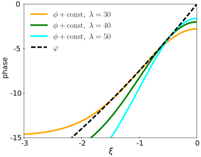
Figure 2: Comparison between the QTM-imprinted phase $\phi(\xi)$ (shifted by a physically irrelevant constant) and ideal-time-reversal phase $\varphi(\xi)$, as given by Eqs. (10) and (11), respectively. The system parameters are the same as in Fig. 1a): $\sigma=1$ and $k=4$. Three different values of the kicking strength are considered: $\lambda=30$ (orange curve), $\lambda=40$ (green curve) and $\lambda=50$ (cyan curve). (The color code coincides with the one adopted in Fig. 1a).)

In order to better understand the quality, underlying principles and limitations of the proposed QTM, it is instructive to compare the state $\Psi_{+}$, rendered by the nonlinear kick (see Eq. (4)), against the desired (perfectly time-reversed) state $\mathcal{C}\Psi_{-}$, obtained by applying the (anti-unitary) complex conjugation operator $\mathcal{C}$ to the pre-kick state $\Psi_{-}$. In the case of the initial state given by Eq. (6), we have

$$\Psi_{+}=\Psi_{-}e^{-i\phi}\,,\qquad\phi=\frac{\lambda}{\sqrt{\pi}\sigma_{1}}e^{-(\xi/\sigma_{1})^{2}}$$ (10)

and

$$\mathcal{C}\Psi_{-}=\Psi_{-}e^{-i(\varphi+\varphi_{0})}\,,\qquad\varphi=\left(\frac{\xi}{\sigma_{1}\sigma}\right)^{2}+2k\xi\,,$$ (11)

where $\sigma_{1}=\sqrt{\sigma^{2}+\sigma^{-2}}$ is the width of wave packet at time $t=1$ when the kick occurs, $\xi=x-k$ is the distance measured from the center of the wave packet, and $\varphi_{0}$ is a constant (position-independent) phase related to the global phase of $\Psi_{-}$. While, in general, the two phases, $\phi$ and $\varphi$, have different functional forms, $\phi(\xi)$ may serve as a reasonable approximation to $\varphi(\xi)$, modulo a physically irrelevant constant shift, over a finite position interval. It is the probability density supported by this position interval that makes the main contribution to the time-reversed wave generated by the nonlinear QTM. Figure 2 presents a comparison between the ideal (target) phase $\varphi(\xi)$ and the phase $\phi(\xi)$ imprinted by the proposed QTM. The system parameters are taken to be the same as in Fig. 1a), i.e. $\sigma=1$ and $k=4$, and the three values of the kicking strength considered are $\lambda=30$, $40$, and $50$.

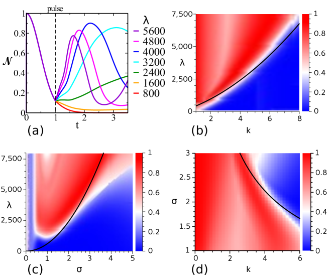
Figure 3: Echo of a 2D Gaussian wave packet subjected to a short, nonlinear pulse. (a) The norm correlation (9) is shown as function of time for varying pulse strength $\lambda$ and fixed momentum $k=4$ and width $\sigma=2$. A norm correlation up to 90% is achievable. Note that the large $\lambda$ values are due to the variable rescaling as described in the text. (b)-(d) The echo peak of the norm correlation is plotted as a function of $\lambda$, $\sigma$ and $k$. The constant parameters are (b) $\sigma=2$, (c) $k=4$ and (d) $\lambda=3000$. The black curves are the analytical approximations by Eq. (14) for the minimal pulse strength $\lambda_{\min}$ required to generate an echo. The radius of the Gaussian ring, is $R=6$.

We further investigate the dynamics of a 2D wave packet, initially given by

$$\Psi_{0}({\bf r})=\sqrt{\frac{1}{2\pi^{3/2}R\sigma}}\exp\left[-\frac{(r-R)^{2}}{2\sigma^{2}}+ikr\right]$$ (12)

with $r=|{\bf r}|$ and $k>0$. For $R\gg\sigma$, the wave function is normalized to one and describes a Gaussian ring of radius $R$ and width $\sigma$ that spreads radially with the average velocity $k$. A straightforward, although tedious, calculation shows that, in the parametric regime defined by $1\ll\sigma\ll R$ and $kR\gg 1$, the wave packet at $t=1^{-}$ has the form (up to a spatially uniform phase) (see Appendix A):

$$\Psi_{-}({\bf r})=\sqrt{\frac{1}{2\pi^{3/2}R_{1}\sigma}}\exp\left[-\frac{(r-R_{1})^{2}}{2\sigma^{2}}+ikr\right]\,,$$ (13)

where $R_{1}=R+k$ is the radius of the Gaussian ring at time $1^{-}$. Thus, the corresponding probability density is given by $\rho=(2\pi^{3/2}R_{1}\sigma)^{-1}\exp[-(r-R_{1})^{2}/\sigma^{2}]$, and the probability current at $t=1^{+}$, reads ${\bf j}_{+}=\left(k\rho+\frac{2\lambda(r-R_{1})}{\sigma^{2}}\rho^{2}\right)\frac{{\bf r}}{r}$. Then, the evaluation of the minimal kick strength required to trigger a probability density echo proceeds in close analogy with the corresponding 1D calculation, resulting in

$$\lambda_{\min}\simeq 2\pi C(R+k)k\sigma^{2}\,.$$ (14)

Finally, just as in the 1D case, the echo time is determined by Eq. (8).

The numerical calculations (Fig. 3) attest the possibility of pronounced echoes up to 90% also in the 2D setup. Although the parameter range is not in the regime of the analytical approximation, the value of $\lambda_{\min}$ in Eq. (14) is still well-suited to estimate the minimal pulse strength $\lambda$ required (see black curves).

The color plots in Figs. 1 and 3 seem to imply $\lambda>\lambda_{\min}$ (marked as black lines) to be the only echo requirement for echo generation. However for large $\lambda$ the wave packet splits into many peaks, as shown in Fig. 1b), blue curve for $\lambda=200$. In such a scenario the norm correlation is still fairly high, but the wave packet might not longer have the desired shape. The effect of many peaks, i.e. very large $\lambda$, on the norm correlation can be seen in Fig. 3c), where the echo strength moderately declines for $\sigma\approx 1$ and $\lambda>3000$.

IV Summary and conclusions

In summary, we have proposed a protocol for simulating the time-reversed motion of a localized matter-wave packet evolving in free space. Our method is based on making a near-instantaneous spatially-homogeneous perturbation to the wave packet dynamics by externally switching on a nonlinear perturbation for a short time interval. The analytical and numerical considerations presented in our paper demonstrate the efficiency of the proposed quantum time mirror in one and two spatial dimensions.

We note that the time reversal protocol proposed in this paper could in principle be employed in different physical systems, such as ultracold atomic clouds, optical pulses, or shallow water waves, as long as the system’s time evolution is governed by the nonlinear Schrödinger equation. Here, we further explore the possible connection between the numerical simulations reported in this paper and relevant atom-optics experiments. To this end, we provide an estimate for values of the dimensionless parameters $\sigma$ and $k$, defined in Eqs. (6) and (12), for the case of ultracold lithium atoms. The mass of a ⁷Li atom is $m=7.016\,\mathrm{u}=1.165\times 10^{-26}\,\mathrm{kg}$. Taking the wave packet propagation time until the nonlinear kick to be $t_{0}=10\,\mathrm{ms}$, we see that the wave packet width range of $10-50\,\mu\mathrm{m}$ corresponds to $1.05<\sigma<5.26$, and the mean velocity range of $2-10\,\mathrm{mm\,s^{-1}}$ corresponds to $2.1<k<10.5$. These parameter ranges coincide with the ones considered in this paper, which strongly suggests that the matter wave reversal effects predicted here can be realized in experiments with lithium BECs.

In order to further facilitate experimental realization of the proposed QTM, we make a rough estimate of the scattering length of condensed lithium atoms required to generate a reflected wave. In the one-dimensional case, the (dimensional) kicking strength $\lambda\hbar\sqrt{\hbar t_{0}/m}/\Delta t$ (see the discussion preceding Eq. (2)) is approximately equal to $2N\hbar^{2}a_{s}/(ma_{\perp}^{2})$, where $N$ is the number of condensed atoms, $a_{s}$ is the scattering length, $\Delta t$ is the kick duration (taken to be $\Delta t=0.001t_{0}=10\,\mu\mathrm{s}$ in our numerical simulations), and $a_{\perp}$ is the linear length scale of the potential confining the atomic motion in the transverse direction Salasnich et al. (2002). This yields the estimate $a_{s}=\lambda a_{\perp}^{2}\sqrt{mt_{0}/\hbar}/(2N\Delta t)$. Taking $N=10^{7}$, $a_{\perp}=10\,\mu\mathrm{m}$, and $\lambda$ in the range $10-200$ (see, e.g., Fig. 1), we find the required scattering length to lie in the range $5\,n\mathrm{m}\lesssim a_{s}\lesssim 105\,n\mathrm{m}$. While challenging, the suggested parameter values are not impossible to achieve in modern atom-optics experiments, using, for instance, such novel techniques as optical control of Feshbach resonances Clark et al. (2015).

Appendix A Free spreading of a Gaussian ring wave packet in 2D: Derivation of Eq. (13)

Let us consider a two-dimensional wave packet, initially (at $t=t_{0}$) given by

$$\Psi_{0}({\bf r})=C\exp\left(-\frac{(r-R)^{2}}{2\sigma^{2}}+ik_{0}(r-R)\right)$$

with $r=|{\bf r}|=\sqrt{x^{2}+y^{2}}$, $\sigma\ll R$, $k_{0}>0$ and $C\simeq 1/\sqrt{2\pi^{3/2}R\sigma}$, so that the probability density is normalized to unity. Let $\Psi({\bf r},t)$ be the wave packet evolved from $\Psi_{0}({\bf r})$ in the course of a free-particle evolution through time $t$. Here, we would like to show that in the parametric regime given by $\sqrt{\hbar t/m}\ll\sigma\ll R$ and $k_{0}R\gg 1$ the wave packet $\Psi$ has the same functional dependence on ${\bf r}$ as $\Psi_{0}$.

The free-particle propagator in 2D reads

$$K_{0}({\bf r},{\bf r}^{\prime},t)=\frac{m}{2\pi i\hbar t}\exp\left(i\frac{m({\bf r}-{\bf r}^{\prime})^{2}}{2\hbar t}\right)\,.$$

Hence,

$$\Psi({\bf r},t) =\frac{mC}{2\pi i\hbar t}\int\,{\rm d}^{2}{\bf r}^{\prime}\exp\left(-\frac{(r^{\prime}-R)^{2}}{2\sigma^{2}}+ik_{0}(r^{\prime}-R)+i\frac{m({\bf r}-{\bf r}^{\prime})^{2}}{2\hbar t}\right)$$

$$=\frac{mC}{2\pi i\hbar t}\int_{0}^{\infty}\,{\rm d}r^{\prime}r^{\prime}\int_{0}^{2\pi}\,{\rm d}\theta\,\exp\left(-\frac{(r^{\prime}-R)^{2}}{2\sigma^{2}}+ik_{0}(r^{\prime}-R)+i\frac{m(r^{2}+r^{\prime 2}-2rr^{\prime}\cos\theta)}{2\hbar t}\right)$$

$$=\frac{mC}{i\hbar t}\exp\left(-\frac{R^{2}}{2\sigma^{2}}-ik_{0}R+i\frac{mr^{2}}{2\hbar t}\right)G(r,t)\,,$$

where

$$G(r,t)=\int_{0}^{\infty}\,{\rm d}r^{\prime}r^{\prime}J_{0}\left(\frac{mrr^{\prime}}{\hbar t}\right)\exp\left[-\frac{1}{2}\left(\frac{1}{\sigma^{2}}-i\frac{m}{\hbar t}\right)r^{\prime 2}+\left(\frac{R}{\sigma^{2}}+ik_{0}\right)r^{\prime}\right]\,.$$

Let us investigate the behavior of $G(r,t)$ around the spatial point $R+\frac{\hbar k_{0}}{m}t$. Taking into account the fact that the main contribution to the integral comes from the region $|r^{\prime}-R|\lesssim\sigma$, we have

$$\frac{mrr^{\prime}}{\hbar t}\sim\frac{mR}{\hbar t}\left(R+\frac{\hbar k_{0}}{m}t\right)=\frac{mR^{2}}{\hbar t}+k_{0}R>k_{0}R\,.$$

Assuming $k_{0}R\gg 1$, we see that the argument of the Bessel function is always large compared to one, i.e.  $\frac{mrr^{\prime}}{\hbar t}\gg 1$. This allows us to use the large argument asymptotics

$$J_{0}\left(\frac{mrr^{\prime}}{\hbar t}\right)\simeq\sqrt{\frac{2}{\pi\frac{mrr^{\prime}}{\hbar t}}}\cos\left(\frac{mrr^{\prime}}{\hbar t}-\frac{\pi}{4}\right)=\sqrt{\frac{\hbar t}{2\pi mrr^{\prime}}}\left[e^{i\left(\frac{mrr^{\prime}}{\hbar t}-\frac{\pi}{4}\right)}+e^{-i\left(\frac{mrr^{\prime}}{\hbar t}-\frac{\pi}{4}\right)}\right]$$

to write

$$\Psi({\bf r},t)\simeq\frac{C}{i}\sqrt{\frac{mR}{2\pi\hbar tr}}\exp\left(-\frac{R^{2}}{2\sigma^{2}}-ik_{0}R+i\frac{mr^{2}}{2\hbar t}\right)\left[\Phi_{+}(r,t)+\Phi_{-}(r,t)\right]\,.$$

Here,

$$\Phi_{\pm}(r,t) =e^{\mp i\frac{\pi}{4}}\int_{-\infty}^{+\infty}\,{\rm d}r^{\prime}\sqrt{\frac{r^{\prime}}{R}}\exp\left\{-\frac{1}{2}\left(\frac{1}{\sigma^{2}}-i\frac{m}{\hbar t}\right)r^{\prime 2}+\left[\frac{R}{\sigma^{2}}+i\left(k_{0}\pm\frac{mr}{\hbar t}\right)\right]r^{\prime}\right\}$$

$$\simeq e^{\mp i\frac{\pi}{4}}\int_{-\infty}^{+\infty}\,{\rm d}r^{\prime}\exp\left\{-\frac{1}{2}\left(\frac{1}{\sigma^{2}}-i\frac{m}{\hbar t}\right)r^{\prime 2}+\left[\frac{R}{\sigma^{2}}+i\left(k_{0}\pm\frac{mr}{\hbar t}\right)\right]r^{\prime}\right\}$$

$$=e^{\mp i\frac{\pi}{4}}\sqrt{\frac{2\pi}{\frac{1}{\sigma^{2}}-i\frac{m}{\hbar t}}}\exp\frac{\left[\frac{R}{\sigma^{2}}+i\left(k_{0}\pm\frac{mr}{\hbar t}\right)\right]^{2}}{2\left(\frac{1}{\sigma^{2}}-i\frac{m}{\hbar t}\right)}\,.$$

Introducing

$$\epsilon=\frac{\hbar t}{m\sigma^{2}}\quad\mathrm{and}\quad v_{0}=\frac{\hbar k_{0}}{m}\,,$$

we rewrite the previous expression as

$$\Phi_{\pm}(r,t)=e^{\mp i\frac{\pi}{4}}\sqrt{\frac{2\pi i\hbar t}{m(1+i\epsilon)}}\exp\left(i\frac{m}{2\hbar t}\frac{[\epsilon R+i(v_{0}t\pm r)]^{2}}{1+i\epsilon}\right)\,.$$

This leads to

$$\Psi({\bf r},t) =\frac{C}{i}\sqrt{\frac{mR}{2\pi\hbar tr}}\exp\left(\frac{m}{2\hbar t}[-\epsilon R^{2}-2iRv_{0}t+ir^{2}]\right)\left[\Phi_{+}(r,t)+\Phi_{-}(r,t)\right]$$

$$=C\sqrt{\frac{R}{i(1+i\epsilon)r}}\sum_{\gamma=\pm 1}e^{-i\gamma\frac{\pi}{4}}\exp\left\{\frac{m}{2\hbar t}\left(-\epsilon R^{2}-2iRv_{0}t+ir^{2}+i\frac{[\epsilon R+i(v_{0}t+\gamma r)]^{2}}{1+i\epsilon}\right)\right\}$$

$$=C\sqrt{\frac{R}{i(1+i\epsilon)r}}\sum_{\gamma=\pm 1}e^{-i\gamma\frac{\pi}{4}}\exp\left(-\frac{m}{2\hbar t}\,\frac{\epsilon(R+\gamma r)^{2}+i\big{[}2(R+\gamma r)+v_{0}t\big{]}v_{0}t}{1+i\epsilon}\,\frac{1-i\epsilon}{1-i\epsilon}\right)$$

$$=C\sqrt{\frac{R}{i(1+i\epsilon)r}}\sum_{\gamma=\pm 1}e^{-i\gamma\frac{\pi}{4}}\exp\left(-\frac{m}{2\hbar t}\,\frac{\epsilon(R+v_{0}t+\gamma r)^{2}+i2(R+v_{0}t+\gamma r)v_{0}t-i\big{[}(v_{0}t)^{2}+\epsilon^{2}(R+\gamma r)^{2}\big{]}}{1+\epsilon^{2}}\right)\,.$$

Assuming further that $\epsilon\ll 1$, we have

$$\Psi({\bf r},t) \simeq C\sqrt{\frac{R}{ir}}\sum_{\gamma=\pm 1}e^{-i\gamma\frac{\pi}{4}}\exp\left\{-\frac{m}{2\hbar t}\left[\epsilon(R+v_{0}t+\gamma r)^{2}+i2(R+v_{0}t+\gamma r)v_{0}t-i(v_{0}t)^{2}\right]\right\}$$

$$=C\sqrt{\frac{R}{ir}}\sum_{\gamma=\pm 1}e^{-i\gamma\frac{\pi}{4}}\exp\left(-\frac{(R+v_{0}t+\gamma r)^{2}}{2\sigma^{2}}-ik_{0}(R+v_{0}t+\gamma r)+i\frac{\hbar k_{0}^{2}t}{2m}\right)\,.$$

Taking into account that last expression for $\Psi$ is only valid for $r$ close to $r_{t}$, where

$$r_{t}=R+v_{0}t=R+\frac{\hbar k_{0}t}{m}\,,$$

we see that a contribution of the term with $\gamma=+1$ is negligibly small. Thus we arrive at the following expression for the freely propagated wave function:

$$\Psi({\bf r},t)\simeq\sqrt{\frac{1}{2\pi^{3/2}\sigma r_{t}}}\exp\left(-\frac{(r-r_{t})^{2}}{2\sigma^{2}}+ik_{0}(r-r_{t})+i\frac{\hbar k_{0}^{2}t}{2m}\right)\,.$$

This expression is only valid in the parametric regime defined by

$$\sqrt{\frac{\hbar t}{m}}\ll\sigma\ll R\quad\mathrm{and}\quad k_{0}R\gg 1\,.$$

References

- Loschmidt (1876) J. Loschmidt, “Über den Zustand des Wärmegleichgewichts eines Systems von Körpern mit Rücksicht auf die Schwerkraft,” Sitzungberichte der Akademie der Wissenschaften II, 128 (1876).
- Boltzmann (1877) L. Boltzmann, “Über die Beziehung eines allgemeinen mechanischen Satzes zum zweiten Hauptsatze der Wärmetheorie,” Sitzungberichte der Akademie der Wissenschaften II, 67 (1877).
- Fink (1997) M. Fink, “Time reversed acoustics,” Physics Today 50, 34 (1997).
- Fink (1999) M. Fink, “Time-reversed acoustics,” Sci. Am. 281, 91 (1999).
- Lerosey et al. (2007) G. Lerosey, J. de Rosny, A. Tourin, and M. Fink, “Focusing beyond the diffraction limit with far-field time reversal,” Science 315, 1120 (2007).
- Mosk et al. (2012) A. P. Mosk, A. Lagendijk, G. Lerosey, and M. Fink, “Controlling waves in space and time for imaging and focusing in complex media,” Nat. Phot. 6, 283 (2012).
- Bacot et al. (2016) V. Bacot, M. Labousse, A. Eddi, M. Fink, and E. Fort, “Time reversal and holography with spacetime transformations,” Nat. Phys. 12, 972 (2016).
- Fink (1992) M. Fink, “Time reversal of ultrasonic fields. I. Basic principles,” Ultrasonics, Ferroelectrics, and Frequency Control, IEEE Transactions on 39, 555–566 (1992).
- Draeger and Fink (1997) C. Draeger and M. Fink, “One-channel time reversal of elastic waves in a chaotic 2d-silicon cavity,” Phys. Rev. Lett. 79, 407 (1997).
- Lerosey et al. (2004) G. Lerosey, J. de Rosny, A. Tourin, A. Derode, G. Montaldo, and M. Fink, “Time reversal of electromagnetic waves,” Phys. Rev. Lett. 92, 193904 (2004).
- Przadka et al. (2012) A. Przadka, S. Feat, P. Petitjeans, V. Pagneux, A. Maurel, and M. Fink, “Time reversal of water waves,” Phys. Rev. Lett. 109, 064501 (2012).
- Chabchoub and Fink (2014) A. Chabchoub and M. Fink, “Time-reversal generation of rogue waves,” Phys. Rev. Lett. 112, 124101 (2014).
- Pastawski et al. (2007) H. M. Pastawski, E. P. Danieli, H. L. Calvo, and L. E. F. Foa Torres, “Towards a time reversal mirror for quantum systems,” EPL 77, 40001 (2007).
- Calvo and Pastawski (2010) H. L. Calvo and H. M. Pastawski, “Exact time-reversal focusing of acoustic and quantum excitations in open cavities: The perfect inverse filter,” EPL 89, 60002 (2010).
- Moshinsky (1952) M. Moshinsky, “Diffraction in time,” Phys. Rev. 88, 625 (1952).
- Gerasimov and Kazarnovskii (1976) A. S. Gerasimov and M. V. Kazarnovskii, “Possibility of observing nonstationary quantum-mechanical effects by means of ultracold neutrons,” Sov. Phys. JETP 44, 892 (1976).
- Č. Brukner and Zeilinger (1997) Č. Brukner and A. Zeilinger, “Diffraction of matter waves in space and in time,” Phys. Rev. A 56, 3804 (1997).
- Mendonça and Shukla (2002) J. T. Mendonça and P. K. Shukla, “Time refraction and time reflection: Two basic concepts,” Phys. Scripta 65, 160 (2002).
- del Campo et al. (2009) A. del Campo, G. Garcia-Calderón, and J. G. Muga, “Quantum transients,” Phys. Rep. 476, 1 (2009).
- Goussev (2012) A. Goussev, “Huygens-Fresnel-Kirchhoff construction for quantum propagators with application to diffraction in space and time,” Phys. Rev. A 85, 013626 (2012).
- Haslinger et al. (2013) P. Haslinger, N. Dorre, P. Geyer, J. Rodewald, S. Nimmrichter, and M. Arndt, “A universal matter-wave interferometer with optical ionization gratings in the time domain,” Nat. Phys. 9, 144 (2013).
- Goussev (2013) Arseni Goussev, “Diffraction in time: An exactly solvable model,” Phys. Rev. A 87, 053621 (2013).
- Sivan and Pendry (2011a) Y. Sivan and J. B. Pendry, “Time reversal in dynamically tuned zero-gap periodic systems,” Phys. Rev. Lett. 106, 193902 (2011a).
- Sivan and Pendry (2011b) Y. Sivan and J. B. Pendry, “Theory of wave-front reversal of short pulses in dynamically tuned zero-gap periodic systems,” Phys. Rev. A 84, 033822 (2011b).
- Sivan and Pendry (2011c) Y. Sivan and J. B. Pendry, “Broadband time-reversal of optical pulses using a switchable photonic-crystal mirror,” Opt. Express 19, 14502 (2011c).
- Chumak et al. (2010) A. V. Chumak, V. S. Tiberkevich, A. D. Karenowska, A. A. Serga, J. F. Gregg, A. N. Slavin, and B. Hillebrands, “All-linear time reversal by a dynamic artificial crystal,” Nat. Commun. 1, 141 (2010).
- Karenowska et al. (2012) A. D. Karenowska, J. F. Gregg, V. S. Tiberkevich, A. N. Slavin, A. V. Chumak, A. A. Serga, and B. Hillebrands, “Oscillatory energy exchange between waves coupled by a dynamic artificial crystal,” Phys. Rev. Lett. 108, 015505 (2012).
- Martin et al. (2008) J. Martin, B. Georgeot, and D. L. Shepelyansky, “Cooling by time reversal of atomic matter waves,” Phys. Rev. Lett. 100, 044106 (2008).
- Ullah and Hoogerland (2011) A. Ullah and M. D. Hoogerland, “Experimental observation of Loschmidt time reversal of a quantum chaotic system,” Phys. Rev. E 83, 046218 (2011).
- Reck et al. (2017) P. Reck, C. Gorini, A. Goussev, V. Krueckl, M. Fink, and K. Richter, “Dirac quantum time mirror,” Phys. Rev. B 95, 165421 (2017).
- Inouye et al. (1998) S. Inouye, M. R. Andrews, J. Stenger, H.-J. Miesner, D. M. Stamper-Kurn, and W. Ketterle, “Observation of feshbach resonances in a bose–einstein condensate,” Nature 392, 151 (1998).
- Roberts et al. (1998) J. L. Roberts, N. R. Claussen, Jr. James P. Burke, C. H. Greene, E. A. Cornell, and C. E. Wieman, “Resonant magnetic field control of elastic scattering in cold 85Rb,” Phys. Rev. Lett. 81, 5109 (1998).
- Krückl (2013) V. Krückl, Wave packets in mesoscopic systems: From time-dependent dynamics to transport phenomena in graphene and topological insulators, Ph.D. thesis, Universität Regensburg, Regensburg, Germany (2013), the basic version of the algorithm is available at TQT Home [http://www.krueckl.de/#en/tqt.php].
- Lanczos (1950) C. Lanczos, “An iteration method for the solution of the eigenvalue problem of linear differential and integral operators,” J. Res. Natl. Bur. Stand. 45, 255 (1950).
- Eckhardt (2003) B. Eckhardt, “Echoes in classical dynamical systems,” J. Phys. A: Math. Gen. 36, 371 (2003).
- Salasnich et al. (2002) L. Salasnich, A. Parola, and L. Reatto, “Effective wave equations for the dynamics of cigar-shaped and disk-shaped bose condensates,” Phys. Rev. A 65, 043614 (2002).
- Clark et al. (2015) L. W. Clark, L. Ha, C. Xu, and C. Chin, “Quantum dynamics with spatiotemporal control of interactions in a stable bose-einstein condensate,” Phys. Rev. Lett. 115, 155301 (2015).