The Herschel$-$ATLAS: magnifications and physical sizes of $500\,\micron$-selected strongly lensed galaxies

Abstract

We perform lens modelling and source reconstruction of Submillimeter Array (SMA) data for a sample of 12 strongly lensed galaxies selected at 500$\micron$ in the Herschel Astrophysical Terahertz Large Area Survey (H-ATLAS). A previous analysis of the same dataset used a single Sérsic profile to model the light distribution of each background galaxy. Here we model the source brightness distribution with an adaptive pixel scale scheme, extended to work in the Fourier visibility space of interferometry. We also present new SMA observations for seven other candidate lensed galaxies from the H-ATLAS sample. Our derived lens model parameters are in general consistent with previous findings. However, our estimated magnification factors, ranging from 3 to 10, are lower. The discrepancies are observed in particular where the reconstructed source hints at the presence of multiple knots of emission. We define an effective radius of the reconstructed sources based on the area in the source plane where emission is detected above 5$\sigma$. We also fit the reconstructed source surface brightness with an elliptical Gaussian model. We derive a median value $r_{\rm eff}\sim 1.77\,$kpc and a median Gaussian full width at half maximum $\sim 1.47\,$kpc. After correction for magnification, our sources have intrinsic star formation rates SFR$\,\sim 900-3500\,{\rm M}_{\sun}{\rm yr}^{-1}$, resulting in a median star formation rate surface density $\Sigma_{\rm SFR}\sim 132\,{\rm M}_{\sun}{\rm yr}^{-1}\,$kpc^-2 (or $\sim 218\,{\rm M}_{\sun}{\rm yr}^{-1}\,$kpc^-2 for the Gaussian fit). This is consistent with what observed for other star forming galaxies at similar redshifts, and is significantly below the Eddington limit for a radiation pressure regulated starburst.

1 Introduction

The samples of strongly lensed galaxies generated by wide-area extragalactic surveys performed at sub-millimetre (sub-mm) to millimetre (mm) wavelengths (Negrello et al., 2010, 2017; Wardlow et al., 2013; Vieira et al., 2013; Planck Collaboration et al., 2015; Nayyeri et al., 2016), with the Herschel space observatory (Pilbratt et al., 2010), the South Pole Telescope (Carlstrom et al., 2011) and the Planck satellite (Cañameras et al., 2015) provide a unique opportunity to study and understand the physical properties of the most violently star forming galaxies at redshifts $z>1$. In fact, the magnification induced by gravitational lensing makes these objects extremely bright and, therefore, excellent targets for spectroscopic follow-up observations aimed at probing the physical conditions of the interstellar medium in the distant Universe (e.g. Valtchanov et al., 2011; Lupu et al., 2012; Harris et al., 2012; Omont et al., 2011, 2013; Oteo et al., 2017a; Yang et al., 2016). At the same time, the increase in the angular sizes of the background sources due to lensing allows us to explore the structure and dynamics of distant galaxies down to sub-kpc scales (e.g. Swinbank et al., 2010, 2015; Rybak et al., 2015; Dye et al., 2015).

In order to be able to fully exploit these advantages, it is crucial to reliably reconstruct the background galaxy from the observed lensed images. The process of source reconstruction usually implies 2an analytic assumption about the surface brightness of the source, for example by adopting Sérsic or Gaussian profiles (e.g Bolton et al., 2008; Bussmann et al., 2013, 2015; Calanog et al., 2014; Spilker et al., 2016). However this approach can be risky, particularly for objects with often complex, clumpy, morphologies like those exhibited by sub-mm/mm selected dusty star forming galaxies (DSFG) when observed at resolutions of tens of milliarcseconds (e.g. Swinbank et al., 2010, 2011; Dye et al., 2015).

Sophisticated lens modelling and source reconstruction techniques have recently been developed to overcome this problem. Wallington et al. (1996) introduced the idea of a pixellated background source, where each pixel value is treated as an independent parameter, thus avoiding any assumption on the shape of the source surface brightness distribution. Warren & Dye (2003) showed that with this approach the problem of reconstructing the background source, for a fixed lens mass model, is reduced to the inversion of a matrix. The best-fitting lens model parameters can then be explored via standard Monte Carlo techniques. In order to avoid unphysical solutions, the method introduces a regularization term that forces a certain degree of smoothness in the reconstructed source. The weight assigned to this regularization term is set by Bayesian analysis (Suyu et al., 2006). Further improvements to the method include pixel sizes adapting to the lens magnification pattern (Dye & Warren, 2005; Vegetti & Koopmans, 2009; Nightingale & Dye, 2015) and non-smooth lens mass models (Vegetti & Koopmans, 2009; Hezaveh et al., 2016) in order to detect dark matter sub-structures in the foreground galaxy acting as the lens.

The method has been extensively implemented in the modelling of numerous lensed galaxies observed with instruments such as the Hubble Space Telescope and the Keck telescope (e.g. Treu & Koopmans, 2004; Koopmans et al., 2006; Vegetti et al., 2010; Dye et al., 2008; Dye et al., 2014, 2015). For DSFGs, high resolution imaging data usable for lens modelling can mainly be achieved by interferometers at the sub-mm/mm wavelengths where these sources are bright. Since the lensing galaxy is usually a massive elliptical, there is virtually no contamination from the lens at those wavelengths. However, an interferometer does not directly measure the surface brightness of the source, but instead it samples its Fourier transform, named the visibility function. As such, the lens modelling of interferometric images needs to be carried out in Fourier space in order to minimize the effect of correlated noise in the image domain and to properly account for the undersampling of the signal in Fourier space, which produces un-physical features in the reconstructed image.

Here, we start from the adaptive source pixel scale method of Nightingale & Dye (2015) and extend it to work directly in the Fourier space to model the Sub-Millimeter Array (SMA) observations of a sample of 12 lensed galaxies discovered in the Herschel Astrophysical Terahertz Large Area Survey (H-ATLAS Eales et al., 2010); eleven of these sources were previously modelled by Bussmann et al. (2013, B13 hereafter) assuming a Sérsic profile for the light distribution of the background galaxy. We reassess their findings with our new approach and also present SMA follow-up observations of 7 more candidate lensed galaxies from the H-ATLAS (Negrello et al., 2017), although we attempted lens modelling for only one of them, where multiple images can be resolved in the data.

The paper is organized as follows: Section 2 presents the sample and the SMA observations. Section 3 describes the methodology used for the lens modeling and its application to interferometric data. In Section 4 we present and discuss our findings, with respect to the results of B13 and other results from the literature. Conclusions are summarized in Section 5. Throughout the paper we adopt the Planck13 cosmology (Planck Collaboration et al., 2014), with H${}_{0}=67$ km s^-1 Mpc^-1, $\Omega_{m}=0.32$, $\Omega_{\Lambda}=0.68$, and assume a Kroupa (2001) initial mass function.

Table 1: List of H-ATLAS lensed galaxies with SMA imaging data selected for the lens modelling and source reconstruction. Most are taken from Bussmann et al. (2013), excluding group/cluster scale lenses and sources which are not clearly resolved into multiple images by the SMA. The list also includes candidate lensed galaxies from N17 for which we have obtained new SMA observations. However only one of them is clearly resolved into multiple images because of the limited resolution achieved and therefore only this object, HATLAS J120127.6-014043, is considered for the lens modelling. Reading from left to right, columns following the identifier are: redshifts of the lens and of the background galaxy (from N17; when no spectroscopic redshift is available the photometric one is provided instead, in italic style), SPIRE/Herschel flux densities at 250, 350 and 500$\micron$ (from N17), flux density from the SMA, array configuration of the observations performed with the SMA (SUB$=$sub-compact, COM$=$compact, EXT$=$extended, VEX$=$very extended).

H-ATLAS IAU Name	$z_{\rm opt}$	$z_{\rm sub-mm}$	$F_{250}$	$F_{350}$	$F_{500}$	$F_{\rm SMA}$	SMA Array
			(mJy)	(mJy)	(mJy)	(mJy)	Configuration
SMA data from Bussmann et al. (2013)
HATLASJ083051.0+013225	0.6261+1.0002	3.634	248.5$\pm$7.5	305.3$\pm$8.1	269.1$\pm$8.7	76.6$\pm$2.0	COM+EXT
HATLASJ085358.9+015537	-	2.0925	396.4$\pm$7.6	367.9$\pm$8.2	228.2$\pm$8.9	50.6$\pm$2.6	COM+EXT+VEX
HATLASJ090740.0$-$004200	0.6129	1.577	477.6$\pm$7.3	327.9$\pm$8.2	170.6$\pm$8.5	20.3$\pm$1.8	COM+EXT
HATLASJ091043.0$-$000322	0.793	1.786	420.8$\pm$6.5	370.5$\pm$7.4	221.4$\pm$7.8	24.4$\pm$1.8	COM+EXT+VEX
HATLASJ125135.3+261457	-	3.675	157.9$\pm$7.5	202.3$\pm$8.2	206.8$\pm$8.5	64.5$\pm$3.4	COM+EXT
HATLASJ125632.4+233627	0.2551	3.565	209.3$\pm$7.3	288.5$\pm$8.2	264.0$\pm$8.5	85.5$\pm$5.6	COM+EXT
HATLASJ132630.1+334410	0.7856	2.951	190.6$\pm$7.3	281.4$\pm$8.2	278.5$\pm$9.0	48.3$\pm$2.1	EXT
HATLASJ133008.4+245900	0.4276	3.1112	271.2$\pm$7.2	278.2$\pm$8.1	203.5$\pm$8.5	49.5$\pm$3.4	COM+EXT
HATLASJ133649.9+291800	-	2.2024	294.1$\pm$6.7	286.0$\pm$7.6	194.1$\pm$8.2	37.6$\pm$6.6	SUB+EXT+VEX
HATLASJ134429.4+303034	0.6721	2.3010	462.0$\pm$7.4	465.7$\pm$8.6	343.3$\pm$8.7	55.4$\pm$2.9	COM+EXT+VEX
HATLASJ142413.9+022303	0.595	4.243	112.2$\pm$7.3	182.2$\pm$8.2	193.3$\pm$8.5	101.6$\pm$7.4	COM+EXT+VEX
New SMA observations
HATLASJ120127.6$-$014043	-	3.80$\pm$0.58	67.4$\pm$6.5	112.1$\pm$7.4	103.9$\pm$7.7	52.4$\pm$3.2	COM+EXT
HATLASJ120319.1$-$011253	-	2.70$\pm$0.44	114.3$\pm$7.4	142.8$\pm$8.2	110.2$\pm$8.6	40.4$\pm$2.4	COM+EXT
HATLASJ121301.5$-$004922	0.191$\pm$0.080	2.35$\pm$0.40	136.6$\pm$6.6	142.6$\pm$7.4	110.9$\pm$7.7	23.4$\pm$1.7	COM+EXT
HATLASJ132504.3+311534	0.58$\pm$0.11	2.03$\pm$0.36	240.7$\pm$7.2	226.7$\pm$8.2	164.9$\pm$8.8	35.2$\pm$2.2	COM
HATLASJ133038.2+255128	0.20$\pm$0.15	1.82$\pm$0.34	175.8$\pm$7.4	160.3$\pm$8.3	104.2$\pm$8.8	19.1$\pm$1.9	COM
HATLASJ133846.5+255054	0.42$\pm$0.10	2.49$\pm$0.42	159.0$\pm$7.4	183.1$\pm$8.2	137.6$\pm$9.0	27.4$\pm$2.5	COM
HATLASJ134158.5+292833	0.217$\pm$0.015	1.95$\pm$0.35	174.4$\pm$6.7	172.3$\pm$7.7	109.2$\pm$8.1	20.9$\pm$1.5	COM

2 Sample and SMA data

2.1 Sample selection

Our starting point is the sample of candidate lensed galaxies presented in Negrello et al. (2017, N17 hereafter) which comprises 80 objects with $F_{500}\geq 100\,$mJy extracted from the full H-ATLAS survey. We kept only the sources in that sample with available SMA 870$\,\mu$m continuum follow-up observations, which are presented in B13 (but see also Negrello et al., 2010; Bussmann et al., 2012). There are 21 in total. We excluded three cluster scale lenses for which the lens modelling is complicated by the need for three or more mass models for the foreground objects (HATLASJ114637.9$-$001132, HATLASJ141351.9$-$000026, HATLASJ132427.0+284449). We also removed those sources where the multiple images are not fully resolved by the SMA and therefore are not usable for source reconstruction, i.e. HATLASJ090302.9$-$014127, HATLASJ091304.9$-$005344, HATLASJ091840.8+023048, HATLASJ113526.2$-$014606, HATLASJ144556.1$-$004853, HATLASJ132859.2+292326. Finally we have not considered in our analysis HATLASJ090311.6+003907, also known as SDP.81, which has been extensively modelled using high resolution data from the Atacama Large Millimetre Array (ALMA Partnership et al., 2015; Rybak et al., 2015; Hatsukade et al., 2015; Swinbank et al., 2015; Tamura et al., 2015; Dye et al., 2015; Hezaveh et al., 2016). We have added an extra source to our sample, HATLASJ120127.6$-$014043, for which we recently obtained new SMA data (see Sec. 2.2). Therefore, our final sample comprises 12 objects, which are included in Table 1.

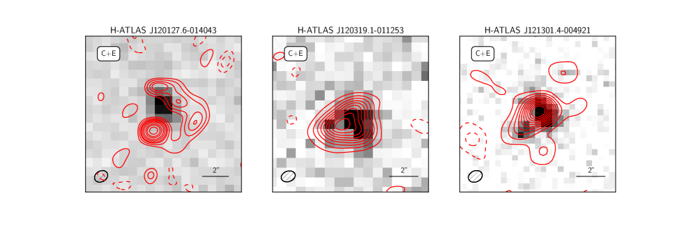
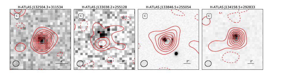
Figure 1: New SMA 870 $\micron$ follow-up observations (red contours, starting at $\pm 2\sigma$ and increasing by factors of two) of seven H-ATLAS candidate lensed galaxies from the N17 sample. The three sources in the top panels were observed in both compact and extended array configurations, while the four sources in the bottom panels only have data obtained in compact configuration. The SMA’s synthesized beam is shown in the lower left corner of each panel. The background images, in grey-scale, show the best available optical/near-IR data and come from the Kilo Degree Survey (KiDS; de Jong et al., 2015, r band at $0.62\,\mu$m for HATLASJ120127.6$-$014043 and HATLASJ121301.4$-$004921), the VISTA Kilo-Degree Infrared Galaxy Survey (VIKING; Edge et al., 2013, K_s band at 2.2 $\micron$ for HATLAS120319.1$-$011253), the UK Infrared Deep Sky Survey Large Area Survey (UKIDSS-LAS; Lawrence et al., 2007, K_s band at $2.2\,\mu$m for HATLASJ132504.3+311534 and HATLASJ133038.2+255128; Y band at $1.03\,\mu$m for HATLASJ134158.5+292833) and the HST Wide Field Camera 3 (WFC3) at $1.6\,\mu$m (for HATLASJ133846.5+255054).

2.2 SMA data

The SMA data used here have been presented in B13 [but see also Negrello et al. (2010)]. They were obtained as part of a large proposal carried out over several semesters using different array configurations from compact (COM) to very-extended (VEX), reaching a spatial resolution of $\sim 0.5^{\prime\prime}$, with a typical integration time of one to two hours on-source, per configuration. We refer the reader to B13 for details concerning the data reduction.

Between December 2016 and March 2017 we carried out new SMA continuum observations at 870$\,\mu$m of a further seven candidate lensed galaxies from the N17 sample (proposal ID: 2016B-S003 PI: Negrello). These targets were selected for having a reliable optical/near-IR counterpart with colours and redshift inconsistent with those derived from the Herschel/SPIRE photometry. Therefore they are very likely to be lensing events, where the lens is clearly detected in the optical/near-IR. They are listed in Table 1, and shown in Fig. 1. Since we were awarded B grade tracks, not all of the observations were executed. Thus while all seven sources were observed in COM configuration, only for three did we also obtain data in the extended (EXT) configuration.

Observations of HATLAS120127.6$-$014043, HATLAS120319.1$-$011253, and HATLAS121301.5$-$004922 were obtained in COM configuration (maximum baselines $\sim$77m) on 29 December 2016. The weather was very good and stable, with a mean atmospheric opacity $\tau_{\rm 225GHz}=0.06$ (translating to 1  mm precipitable water vapor). All eight antennas participated, with 6 GHz of continuum bandwidth per sideband in each of two polarizations (for the equivalent of 24 GHz total continuum bandwidth). The central frequency of the observations was 344 GHz (870$\,\mu$m). The target observations were interleaved over a roughly 8 hour transit period, resulting in 100 to 110 minutes of on-source integration time for each target (with the balance spent on bandpass and gain calibration using the bright, nearby radio source 3C273). The absolute flux scale was determined using observations of Callisto. Imaging the visibility data with a natural weighting scheme produced a synthesized beam with full-width at half maximum (FWHM) $\sim 2^{\prime\prime}$, and all three targets were detected with high confidence, with achieved image RMS values of 1.3 mJy beam^-1. Data for these three sources were combined with later higher resolution data (see below).

Observations of HATLASJ132504.3+311534, HATLASJ133038.2+255128, HATLASJ133846.5+255054, HATLASJ134158.5+292833 were obtained in the COM configuration on 02 January 2017. The weather was good and stable, with $\tau_{\rm 225GHz}=0.07$ (corresponding to 1.2 mm precipitable water vapor). All eight antennas participated, with 6 GHz of continuum bandwidth per sideband in each of two polarizations (for the equivalent of 24  GHz total continuum bandwidth). The mean frequency of the observations was 344 GHz (870$\,\mu$m). The target observations were interleaved over a roughly four hour rising to transit period, resulting in 40 minutes of on-source integration time for three targets (HATLASJ134158.5+292833 only received 30 min). Gain calibration was performed using observations of the nearby radio source 3C286, while bandpass and absolute flux scale were determined using observations of Callisto. Imaging the visibility data produced a synthesized beam with ${\rm FWHM}\sim 2^{\prime\prime}$, and all four targets were detected with high confidence, with image RMS values of 1.5-1.7 mJy beam^-1.

HATLAS120127.6$-$014043, HATLAS120319.1$-$011253, and HATLAS121301.5$-$004922 were also observed in the EXT configuration (maximum baselines  220 m) on 29 March 2017. The weather was excellent and fairly stable, with a mean $\tau_{\rm 225GHz}$ of 0.04 rising to 0.05 (translating to 0.65-0.8 mm precipitable water vapor). All eight antennas participated, now with 8 GHz of continuum bandwidth per sideband in each of two polarizations (for the equivalent of 32 GHz total continuum bandwidth); however, on one antenna only one of the two receivers was operational, resulting in a small loss of signal-to-noise ($\sim 3\%$). The mean frequency of the observations was 344 GHz (870$\,\mu$m). The target observations were interleaved over a roughly six hour mostly rising transit period, resulting in 75 to 84 minutes of on-source integration time for each target. Bandpass and phase calibration observations were of 3C273, and the absolute flux scale was determined using observations of Ganymede. These extended configuration data were then imaged jointly with the compact configuration data from 29 December 2016. For each source, the synthesized resolution is roughly $1.0^{\prime\prime}\times 0.8^{\prime\prime}$, and the rms in the combined data maps ranges from 800 to 900 $\mu$Jy beam^-1.

There is evidence of extended structure in several of our new targets, even from the COM data alone (e.g. HATLASJ133038.2+255128 and HATLASJ133846.5+255054); however only in HATLASJ120127.6$-$014043, which benefits from EXT data, are the typical multiple images of a lensing events clearly detected and resolved.
The measured 870 $\micron$ flux density for each source is reported in Table 1. It was computed by adding up the signal inside a customized aperture that encompasses the source emission. The quoted uncertainties correspond to the root-mean-square variation of the primary-beam corrected signal measured within the same aperture in 100 random positions inside the region defined by the primary beam of the instrument.
As explained in Section 3, our lens modelling and source reconstruction are performed on the SMA data by adopting a natural weighting scheme. The SMA dirty images obtained with this scheme are shown in the left panels of Fig. 2.

3 Lens modelling and source reconstruction

In order perform the lens modeling and to reconstruct the intrinsic morphology of the background galaxy, we follow the Regularized Semilinear Inversion (SLI) method introduced by Warren & Dye (2003), which assumes a pixelated source brightness distribution. It also introduces a regularization term to control the level of smoothness of the reconstructed source. The method was improved by Suyu et al. (2006) using Bayesian analysis to determine the optimal weight of the regularization term and by Nightingale & Dye (2015) with the introduction of a source pixelization that adapts to the lens model magnification. Here we adopt all these improvements and extend the method to deal with interferometric data.
We provide below a summary of the SLI method, but we refer the reader to Warren & Dye (2003) for more details.

3.1 The adaptive semilinear inversion method

The image plane (IP) and the source plane (SP), i.e. the planes orthogonal to the line-of-sight of the observer to the lens containing the lensed images and the background source, respectively, are gridded into pixels whose values represent the surface brightness counts. In the IP, the pixel values are described by an array of elements $d_{j}$, with $j=1,...,J$, and associated statistical uncertainty $\sigma_{j}$, while in the SP the unknown surface brightness counts are represented by the array of elements $s_{i}$, with $i=1,...,I$. For a fixed lens mass model, the image plane is mapped to the source plane by a unique rectangular matrix $f_{ij}$. The matrix contains information on the lensing potential, via the deflection angles, and on the smearing of the images due to convolution with a given point spread function (PSF). In practice, the element $f_{ij}$ corresponds to the surface brightness of the $j$-th pixel in the lensed and PSF-convolved image of source pixel $i$ held at unit surface brightness. The vector, S, of elements $s_{i}$ that best reproduces the observed IP is found by minimizing the merit function

$$G=\frac{1}{2}\chi^{2}=\frac{1}{2}\sum_{j=1}^{J}\left(\dfrac{\sum_{i=1}^{I}s_{i}f_{ij}-d_{j}}{\sigma_{j}}\right)^{2}.$$ (1)

It is easy to show that the solution to the problem satisfies the matrix equation

$$\textbf{F}\cdot\textbf{S}=\textbf{D},$$ (2)

where D is the array of elements $D_{i}=\sum_{j=1}^{J}(f_{ij}d_{j})/\sigma_{j}^{2}$ and F is a symmetric matrix of elements $F_{ik}=\sum_{j=1}^{J}(f_{ij}f_{kj})/\sigma_{j}^{2}$. Therefore, the most likely solution for the source surface brightness counts can be obtained via a matrix inversion

$$\textbf{S}=\textbf{F}^{-1}\textbf{D}.$$ (3)

However, in this form, the method may produce unphysical results. In fact, each pixel in the SP behaves independently from the others and, therefore, the reconstructed source brightness profile may show severe discontinuities and pixel-to-pixel variations due to the noise in the image being modelled. In order to overcome this problem a prior on the parameters $s_{i}$ is assumed, in the form of a regularization term, $E_{\rm reg}$, which is added to the merit function in Eq. (1). This forces a smooth variation in the value of nearby pixels in the SP:

$$G_{\lambda}=\frac{1}{2}\chi^{2}+\lambda E_{\rm reg}=\frac{1}{2}\chi^{2}+\lambda\frac{1}{2}\textbf{S}^{T}\textbf{H}\textbf{S},$$ (4)

where $\lambda$ is a regularization constant, which controls the strength of the regularization, and H is the regularization matrix. We have chosen a form for the regularization term $E_{\rm reg}$ that preserves the matrix formalism [see Eq. (9)]. The minimum of the merit function in Eq. (4) satisfies the condition

$$[\textbf{F}+\lambda\textbf{H}]\cdot\textbf{S}=\textbf{D},$$ (5)

and, therefore, can still be derived via a matrix inversion

$$\textbf{S}=[\textbf{F}+\lambda\textbf{H}]^{-1}\textbf{D}.$$ (6)

The presence of the regularization term ensures the existence of a physical solution for any sensible regularization scheme.
The value of the regularization constant is found by maximizing the Bayesian evidence $\epsilon$ (Suyu et al., 2006)

$$2\ln{[\epsilon(\lambda)]} = -G_{\lambda}(\textbf{S})-\ln[\det(\textbf{F}+\lambda\textbf{H})]$$ (7)

$$+\ln[\det(\lambda\textbf{H})]-\sum_{j=1}^{J}\ln{(2\pi\sigma_{j}^{2})},$$

S representing here the set of $s_{i}$ values obtained from Eq. (6) for a given $\lambda$.
The errors on the reconstructed source surface brightness distribution, for a fixed mass model, are given by the diagonal terms of the covariance matrix (Warren & Dye, 2003):

$$\sigma_{ik}^{2}=\sum_{j=1}^{J}\sigma_{j}^{2}\dfrac{\partial s_{i}}{\partial d_{j}}\dfrac{\partial s_{k}}{\partial d_{j}}=R_{ik}-\lambda\sum_{l=1}^{I}R_{il}[\textbf{R}\textbf{H}]_{kl},$$ (8)

where $\textbf{R}=[\textbf{F}+\lambda\textbf{H}]^{-1}$. We use this expression to draw signal-to-noise ratio contours in the reconstructed SP in Fig. 2 for the best fit lens model.

Eqs (6)-(8) allow us to derive the SP solution for a fixed lens mass model. However the parameters that best describe the mass distribution of the lens are also to be determined. This is achieved by exploring the lens parameter space and computing each time the evidence in Eq. (8) marginalized over $\lambda$, i.e. $\epsilon=\int\epsilon(\lambda)P(\lambda)d\lambda$, where $P(\lambda)$ is the probability distribution of the values of the regularization constant for a given lens model. The best-fitting values of the lens model parameters are those that maximize $\epsilon$. We follow Suyu et al. (2006) by approximating $P(\lambda)$ with a delta function centered around the value $\tilde{\lambda}$ that maximizes Eq. (8), so that $\epsilon\simeq\epsilon(\tilde{\lambda})$.

The pixels in the SP that are closer to the lens caustics are multiply imaged over different regions in the IP, and therefore benefit from better constraints during the source reconstruction process, compared to pixels located further away from the same lines. As a consequence, the noise in the reconstructed source surface brightness distribution significantly varies across the SP. At the same time, in highly magnified regions of the SP the information on the source properties at sub-pixel scales is not fully exploited. In order to overcome this issue we follow the adaptive SP pixelization scheme proposed by Nightingale & Dye (2015). For a fixed mass model the IP pixel centres are traced back to the SP and a k-means clustering algorithm is used to group them and to define new pixel centres in the SP. These centres are then used to generate Voronoi cells, mainly for visualization purposes. Within this adaptive pixelization scheme we use a gradient regularization term defined as:

$$E_{\rm reg}=\sum_{i=1}^{I}\sum_{k=1}^{N_{v}(i)}(s_{i}-s_{k})^{2}$$ (9)

where $N_{v}(i)$ are the counts members of the set of Voronoi cells that share at least one vertex with the $i$-th pixel.

3.2 Modeling in the uv plane

We extend the adaptive SLI formalism to deal with images of lensed galaxies produced by interferometers.
An interferometer correlates the signals of an astrophysical source collected by an array of antennas to produce a visibility function $V(u,v)$, that is the Fourier transform of the source surface brightness $I(x,y)$ sampled at a number of locations in the Fourier space, or $uv$-plane:

$$V(u,v)=\int\int A(x,y)I(x,y)e^{-2\pi i(ux+vy)}dxdy$$ (10)

where $A$ is the effective collecting area of each antenna, i.e. the primary beam.
Because of the incomplete sampling of the $uv$-plane the image of the astrophysical source obtained by Fourier transforming the visibility function will be affected by artifacts, such as side-lobes, and by correlated noise. Therefore, a proper source reconstruction performed on interferometric data should be carried out directly in the $uv$-plane.
We define the merit function using the visibility function

$$G_{\lambda} = \frac{1}{2}\sum_{u,v}^{N_{\rm vis}}\left|\frac{V_{\rm model}(u,v)-V_{\rm obs}(u,v)}{\sigma(u,v)}\right|^{2}+\lambda\frac{1}{2}\textbf{S}^{T}\textbf{H}\textbf{S}$$ (11)

$$= \frac{1}{2}\sum_{u,v}^{N_{\rm vis}}\left(\frac{V_{\rm model}^{\mathbb{R}}(u,v)-V_{\rm obs}^{\mathbb{R}}(u,v)}{\sigma(u,v)}\right)^{2}$$

$$+\frac{1}{2}\sum_{u,v}^{N_{\rm vis}}\left(\frac{V_{\rm model}^{\mathbb{I}}(u,v)-V_{\rm obs}^{\mathbb{I}}(u,v)}{\sigma(u,v)}\right)^{2}$$

$$+\lambda\frac{1}{2}\textbf{S}^{T}\textbf{H}\textbf{S},$$

where $N_{\rm vis}$ is the number of observed visibilities $V_{\rm obs}=V_{\rm obs}^{\mathbb{R}}+iV_{\rm obs}^{\mathbb{I}}$, while $\sigma^{2}(u,v)=\sigma_{\rm real}(u,v)^{2}+\sigma_{\rm imag}^{2}(u,v)$, with $\sigma_{\rm real}$ and $\sigma_{\rm imag}$ representing the 1$\sigma$ uncertainty on the real and imaginary parts of $V_{\rm obs}$, respectively. With this definition of the merit function we are assuming a natural weighting scheme for the visibilities in our lens modelling.
Following the formalism of Eq. (1), we can introduce a rectangular matrix of complex elements $\hat{f}_{jk}=\hat{f}^{\mathbb{R}}_{jk}+i\hat{f}^{\mathbb{I}}_{jk}$, with $k=1,..,N_{\rm vis}$ and $j=1,..,N$, $N$ being the number of pixels in the SP. The term $\hat{f}_{jk}$ provides the Fourier transform of a source pixel of unit surface brightness at the $j$-th pixel position and zero elsewhere, calculated at the location of the $k$-th visibility point in the $uv$-plane. The effect of the primary beam is also accounted for in calculating $\hat{f}_{jk}$. Therefore, Eq. (11) can be re-written as

$$G_{\lambda} = \frac{1}{2}\sum_{u,v}^{N_{\rm vis}}\left|\frac{V_{\rm model}(u,v)-V_{\rm obs}(u,v)}{\sigma(u,v)}\right|^{2}+\lambda\frac{1}{2}\textbf{S}^{T}\textbf{H}\textbf{S}$$ (12)

$$= \frac{1}{2}\sum_{k}^{N_{\rm vis}}\left(\frac{\sum_{j=1}^{N}s_{j}\hat{f}^{\mathbb{R}}_{jk}-V_{{\rm obs},k}^{\mathbb{R}}}{\sigma_{k}}\right)^{2}$$

$$+\frac{1}{2}\sum_{k}^{N_{\rm vis}}\left(\frac{\sum_{j=1}^{N}s_{j}\hat{f}^{\mathbb{I}}_{jk}-V_{{\rm obs},k}^{\mathbb{I}}}{\sigma_{k}}\right)^{2}$$

$$+\lambda\frac{1}{2}\textbf{S}^{T}\textbf{H}\textbf{S}.$$

In deriving this expression we have assumed that $\bf{S}$ is an array of real values, as it describes a surface brightness.
The set of $s_{i}$ values that best reproduces the observed IP can then be derived as in Eq (6):

$$\textbf{S}=[\hat{\textbf{F}}+\lambda\textbf{H}]^{-1}\hat{\textbf{D}}.$$ (13)

with the new matrices $\hat{\textbf{F}}$ and $\hat{\textbf{D}}$ defined as follows

$$\hat{\textbf{F}}_{jk}=\sum_{l=1}^{N_{\rm vis}}\frac{\hat{f}^{\mathbb{R}}_{jl}\hat{f}^{\mathbb{R}}_{lk}+\hat{f}^{\mathbb{I}}_{jl}\hat{f}^{\mathbb{I}}_{lk}}{\sigma_{l}^{2}}$$ (14)

$$\hat{\textbf{D}}_{j}=\sum_{l=1}^{N_{\rm vis}}\frac{\hat{f}^{\mathbb{R}}_{jl}V_{{\rm obs},l}^{\mathbb{R}}+\hat{f}^{\mathbb{I}}_{jl}V_{{\rm obs},l}^{\mathbb{I}}}{\sigma_{l}^{2}}$$ (15)

The computation of the regularization constant is exactly as in Eq. (7) with $G_{\lambda}$, F and $\sigma$ replaced by the corresponding quantities defined in this section.

Table 2: Results of the modelling for the lens mass distribution, for which a SIE profile is assumed. The parameters of the model are: the normalization of the profile, expressed in terms of the Einstein radius ($\theta_{\rm E}$); the rotation angle ($\theta_{\rm L}$; measured counter-clockwise from West); the minor-to-major axis ratio ($q_{\rm L}$); the position of the lens centroid from the centre of the images in Fig. 2; the shear strength ($\gamma$) and the shear angle ($\theta_{\gamma}$; counter-clockwise from West).

IAUname	$\theta_{\rm E}$	$\theta_{\rm L}$	$q_{\rm L}$	$\Delta x_{\rm L}$	$\Delta y_{\rm L}$	$\gamma$	$\theta_{\gamma}$
	(arcsec)	(∘)		(arcsec)	(arcsec)		(∘)
HATLASJ083051.0+013225	0.31$\pm$0.03	38.5$\pm$ 7.5	0.33$\pm$0.07	$-$0.49$\pm$0.04	+0.07$\pm$ 0.04	-	-
	0.58$\pm$0.05	172.6$\pm$16.8	0.82$\pm$0.08	+0.18$\pm$0.03	$-$0.63$\pm$0.05	-	-
HATLASJ085358.9+015537	0.54$\pm$0.01	62.3$\pm$30.0	0.95$\pm$0.05	$-$0.22$\pm$0.03	+0.03$\pm$0.03	-	-
HATLASJ090740.0$-$004200	0.65$\pm$0.02	143.7$\pm$ 7.0	0.75$\pm$0.07	$-$0.09$\pm$0.02	$-$0.06$\pm$0.05	-	-
HATLASJ091043.1$-$000321	0.91$\pm$0.03	112.9$\pm$10.2	0.62$\pm$0.09	0.00$\pm$0.07	+0.33$\pm$0.05	0.20$\pm$0.05	76.0$\pm$12.0
HATLASJ120127.6$-$014043	0.82$\pm$0.04	169.0$\pm$6.7	0.58$\pm$0.09	+0.06$\pm$0.06	+2.00$\pm$0.05	-	-
HATLASJ125135.4+261457	1.10$\pm$0.02	28.0$\pm$2.5	0.51$\pm$0.06	$-$0.23$\pm$0.05	+0.39$\pm$0.04	-	-
HATLASJ125632.7+233625	0.69$\pm$0.03	24.6$\pm$7.4	0.54$\pm$0.09	$-$0.05$\pm$0.10	$-$0.10$\pm$0.06	-	-
HATLASJ132630.1+334410	1.76$\pm$0.05	149.4$\pm$9.0	0.62$\pm$0.08	$-$0.49$\pm$0.10	+0.67$\pm$0.10	-	-
HATLASJ133008.4+245900	1.03$\pm$0.02	172.1$\pm$2.2	0.51$\pm$0.03	$-$1.54$\pm$0.08	+0.95$\pm$0.04	-	-
HATLASJ133649.9+291801	0.41$\pm$0.02	38.5$\pm$4.3	0.53$\pm$0.12	+0.22$\pm$0.05	+0.20$\pm$0.04	-	-
HATLASJ134429.4+303036	0.96$\pm$0.01	82.7$\pm$1.5	0.53$\pm$0.07	+0.34$\pm$0.06	+0.02$\pm$0.03	-	-
HATLASJ142413.9+022303	0.98$\pm$0.02	91.0$\pm$4.9	0.79$\pm$0.04	+1.09$\pm$0.03	+0.33$\pm$0.04	-	-

3.3 Lens model

In order to compare our findings with the results presented in B13, we model the mass distribution of the lenses as a Singular Isothermal Ellipsoid (SIE; Kormann et al., 1994), i.e. we assume a density profile of the form $\rho\propto r^{-2}$, $r$ being the elliptical radius. Our choice of a SIE over a more generic power-law profile, $\rho\propto r^{-\alpha}$, is also motivated by the results of the modelling of other lensing systems from literature (e.g. Barnabè et al., 2009; Dye et al., 2014, 2015, 2017), which show that $\alpha\sim 2$, and by the need of keeping to a minimum the number of free parameters. In fact, the resolution of the SMA data analyzed here is a factor $\times 3-4$ worse than the one provided by the optical and near-infrared imaging data $-$ mainly from the Hubble space telescope $-$ used in the aforementioned literature.
However it is important to point out that a degeneracy between different lens model profiles can lead to biased estimates of the source size and magnification. In fact, as first discussed by Falco et al. (1985), a particular rescaling of the density profile of the lens, together with an isotropic scaling of the source plane coordinates, produces exactly the same observed image positions and flux ratios (but different time delays). This is known as the mass-sheet transformation (MST) and represents a special case of the more general source-position transformation described by Schneider & Sluse (2014). Schneider & Sluse (2013) showed that the MST is formally broken by assuming a power-law model for the mass distribution of the lens, although there is no physical reason why the true lens profile should have such an analytic form. Furthermore, the power-law model is also affected by the $\sigma-q-\alpha$ degeneracy between the lens mass (expressed in terms of the 1D velocity dispersion $\sigma$), the axis ratio ($q$) and the slope ($\alpha$). In fact, as discussed in Nightingale & Dye (2015), different combinations of these three parameters produce identical solutions in the image plane, but geometrically scaled solutions in the source plane, thus affecting the measurement of the source size and magnification. However, the same author also showed that the use of a randomly initialized adaptive grid (the same adopted in this work), with a fixed number of degree-of-freedom, removes the biases associated with this degeneracy. We will test our assumption of a SIE profile in a future paper using available HST and ALMA data, by comparing the lens modelling results obtained for $\alpha=2$ with those derived for a generic power-law model (Negrello et al. in prep.).
The SIE profile is described by 5 parameters: the displacement of the lens centroid, $\Delta x_{\rm L}$ and $\Delta y_{\rm L}$, with respect to the centre of the image, the Einstein radius, $\theta_{\rm E}$, the minor-to-major axis ratio, $q_{\rm L}$, the orientation of the semi-major axis, $\theta_{\rm L}$, measured counter-clockwise from West. For simplicity we do not include an external shear unless it is needed to improve the modelling. In that case, its effect is described by two additional parameters: the shear strength, $\gamma$, and the shear angle, $\theta_{\gamma}$, also measured counter-clockwise from West, thus raising the total number of free parameters from 5 to 7.

3.4 Implementation

The lens parameter space is explored using multinest (Feroz & Hobson, 2008; Feroz et al., 2009), a Monte Carlo technique implementing the nested sampling described in Skilling (2006). Flat priors are adopted for the lens model, within the range: $0.1\,{\rm arcsec}\leq\theta_{\rm E}\leq 3.0\,{\rm arcsec}$; $0^{\circ}\leq\theta_{\rm L}<180^{\circ}$; $0.2\leq q_{\rm L}<1.0$; $-0.5\,{\rm arcsec}\leq\Delta x_{\rm L}\leq 0.5\,{\rm arcsec}$; $-0.5\,{\rm arcsec}\leq\Delta y_{\rm L}\leq 0.5\,{\rm arcsec}$; $0.0\leq\gamma\leq 0.3$; $0^{\circ}\leq\theta_{\gamma}<180^{\circ}$. In order to lighten the computational effort, a mask is applied to the IP pixels, keeping only those relevant, i.e. containing the lensed image, with minimum background sky. These are then traced back to the SP where they define the area used for the source reconstruction.
As suggested in N15, a nuisance in lens modeling algorithms is the existence of unrealistic solutions, occupying significant regions of the parameter space where the Monte Carlo method gets stuck. In general these local minima of the evidence correspond to a reconstructed SP that resembles a demagnified version of the observed IP. In order to avoid them, the first search of the parameter space is performed on a selected grid of values of the free parameters, following the methods presented in N15. Then, the regions occupied by unrealistic solutions are excluded from the subsequent search. Once the best lens model parameters are identified, a final multinest run is employed to sample the posterior distribution function (PDF), and to estimate the corresponding uncertainties, which are quoted as the 16th and 84th percentile of the PDF.
A fundamental quantity provided by the lens modelling is the magnification factor, $\mu$. This is defined as the ratio between the total flux density of the source, as measured in the SP, and the total flux density of the corresponding images in the IP. In practice we estimate it as $\mu=F^{\rm IP}_{N\sigma}/F^{\rm SP}_{N\sigma}$ where $F^{\rm SP}_{N\sigma}$ is the flux density contributed by all the pixels in the SP with signal-to-noise ratio ${\rm SNR}\geq N$, while $F^{\rm IP}_{N\sigma}$ is the summed flux density of the all pixels within the corresponding region in the IP. We compute the value of $\mu$ for $N=3$ and $N=5$, taking the latter as our reference case. The uncertainty on the magnification factor is derived by calculating $\mu$ 1000 times, each time perturbing the lens model parameters around their best-fitting values; the final magnification factor is the median of the resulting distribution with errors given by the 16th and 84th percentile of the same distribution.

4 Results and discussion

The best-fitting values of the lens model parameters are reported in Table 2, while the results of the source reconstruction are shown in Fig. 2. The first panel on the left is the SMA dirty image, generated by adopting a natural weighting scheme. The second and the third panels from the left show the reconstructed IP and the residuals, respectively. The latter are derived by subtracting the model visibilities from the observed ones and then imaging the differences. The panel on the right shows the reconstructed source with contours at 3$\sigma$ (black curve) and 5$\sigma$ (white curves), while the second panel from the right shows the image obtained by assuming the best-fitting lens model and performing the gravitational lensing directly on the reconstructed source. The lensed image obtained in this way is unaffected by the sampling of the $uv$ plane and can thus help to recognize in the SMA dirty image those features that are really associated with the emission from the background galaxy.

The estimated magnification factors, $\mu_{3\sigma}$ and $\mu_{5\sigma}$, are listed in Table 3 for the two adopted values of the signal-to-noise ratios in the SP, i.e. SNR$\,\geq 3$ and SNR$\,\geq 5$, respectively. The area, $A_{\rm dust}$, of the regions in the SP used to compute the magnification factors is also listed in the same table together with the corresponding effective radius, $r_{\rm eff}$. The latter is defined as the radius of a circle of area equal to $A_{\rm dust}$. We note that, despite the difference in the value of the area in the two cases, the derived magnification factors are consistent with each other. In fact, as the area decreases when increasing the SNR from 3 to 5, the centre of the selected region, in general, moves away from the caustic, where the magnification is higher. The two effects tend to compensate each other, thus reducing the change in the total magnification. Below we discuss our findings with respect to the results of B13 and other results from the literature.

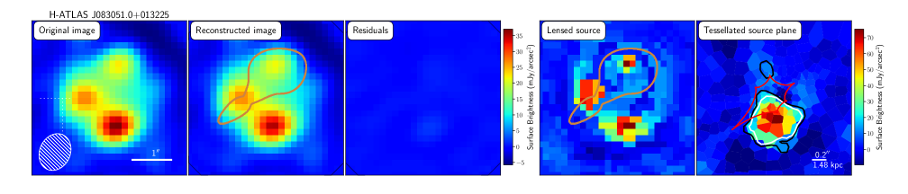
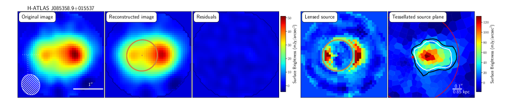
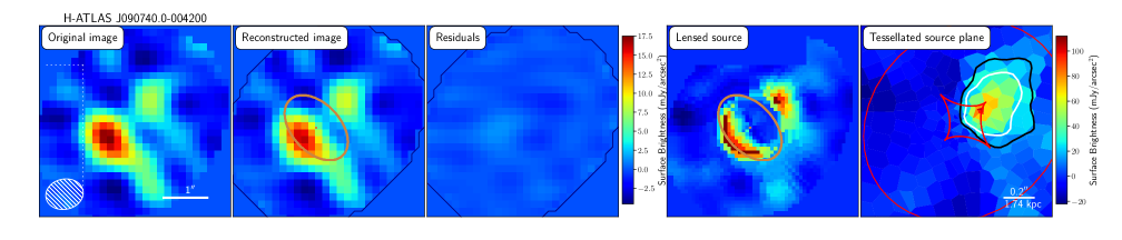
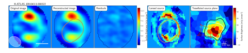
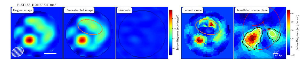
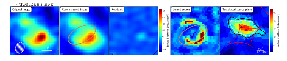
Figure 2: Results of the lens modelling and source reconstruction. From left to right: input SMA image (created using a natural weighting scheme); minimum $\chi^{2}$ image; residuals obtained by first subtracting the observed visibilities with the model ones and then transforming back to the real space; image obtained by lensing the reconstructed source plane using the best-fitting lens model; the reconstructed background source with contours at 3$\,\sigma$ (black curve) and 5$\,\sigma$ (white curve). The caustics and the critical lines are shown in brown (in the second and fourth panels from left) and in red (in the right panel), respectively. The white hatched ellipse in the bottom left corner of the leftmost panels represents the SMA synthesized beam.

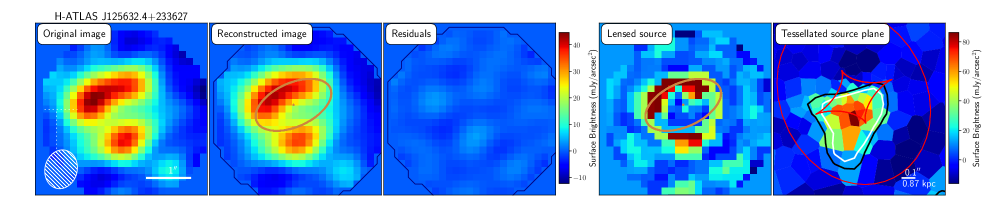
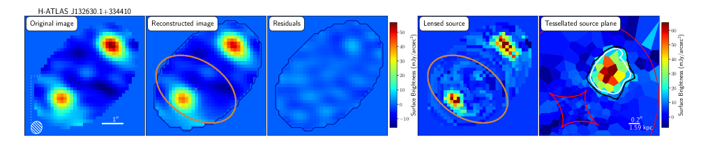
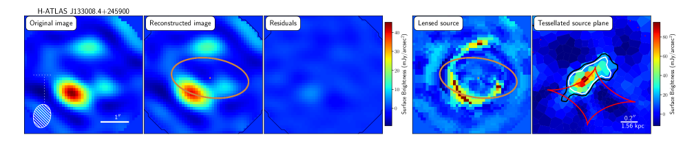
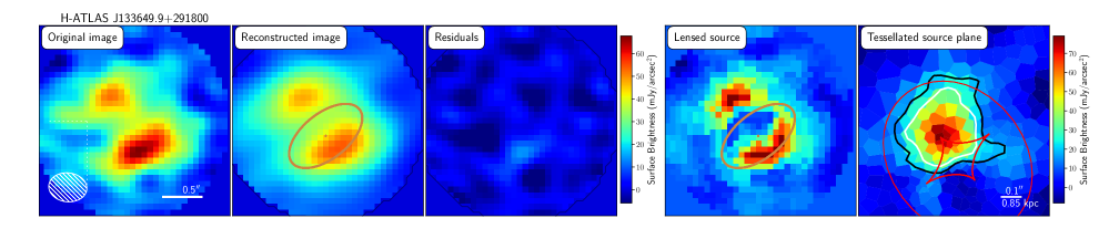
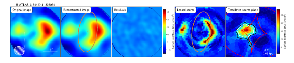
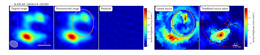
Figure 2: $-$ continued

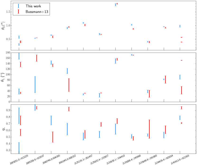
Figure 3: Comparison between our results (blue error bars) and those of B13 (red error bars) for the parameters of the SIE lens mass model: Einstein radius, $\theta_{\rm E}$, rotation angle, $\theta_{\rm L}$, and minor-to-major axis ratio, $q_{\rm L}$. Two datapoints are plotted whenever two lenses are employed in lens modeling (HATLASJ083051.0+013225, HATLASJ142413.9+022303).

Table 3: Lens modeling results: source properties. Magnifications, $\mu_{3\sigma}$ and $\mu_{5\sigma}$, are evaluated as the ratio between the total flux density of the region in the SP with SNR$\geq 3$ and SNR$\geq 5$, respectively, and the total flux density of the corresponding region in the IP. $A_{\rm dust,3\sigma}$ and $A_{\rm dust,5\sigma}$ are the areas of the regions with SNR$\geq 3$ and SNR$\geq 5$ in the source plane, while $r_{\rm eff,3\sigma}$ and $r_{\rm eff,5\sigma}$, are the radius of a circle with area equal to $A_{\rm dust,3\sigma}$ and $A_{\rm dust,5\sigma}$, respectively. FHWMs are the values of the FWHM of the major and minor axis length obtained from the Gaussian fit to the reconstructed source surface brightness, while FWHM${}_{\rm m}=\sqrt{{\rm FWHM_{maj}\times FWHM_{min}}}$.

H-ATLAS IAU name	$\mu_{3\sigma}$	$\mu_{5\sigma}$	$A_{\rm dust,3\sigma}$	$A_{\rm dust,5\sigma}$	$r_{\rm eff,3\sigma}$	$r_{\rm eff,5\sigma}$	FWHMs	FWHMm
			(kpc2)	(kpc2)	(kpc)	(kpc)	(kpc)	(kpc)
HATLASJ083051.0+013225	4.25$\pm$0.68	4.04$\pm$0.70	33.5$\pm$5.6	22.3$\pm$2.8	3.27$\pm$0.27	2.67$\pm$0.17	1.64/1.46	1.54$\pm$0.10
HATLASJ085358.9+015537	5.40$\pm$1.76	5.26$\pm$1.82	16.1$\pm$6.0	9.5$\pm$3.7	2.26$\pm$0.41	1.74$\pm$0.34	1.72/1.14	1.37$\pm$0.33
HATLASJ090740.0$-$004200	6.73$\pm$0.93	7.51$\pm$1.31	18.4$\pm$4.1	10.2$\pm$2.0	2.42$\pm$0.27	1.80$\pm$0.19	1.83/1.24	1.46$\pm$0.18
HATLASJ091043.1$-$000321	6.63$\pm$0.68	6.89$\pm$0.79	10.6$\pm$2.7	5.5$\pm$1.6	1.84$\pm$0.23	1.33$\pm$0.20	1.32/1.17	1.24$\pm$0.19
HATLASJ120127.6$-$014043	3.30$\pm$0.55	3.03$\pm$0.59	33.3$\pm$4.8	17.4$\pm$2.4	3.25$\pm$0.23	2.36$\pm$0.16	1.87/1.33	1.57$\pm$0.07
HATLASJ125135.4+261457	8.38$\pm$0.54	9.16$\pm$0.78	23.3$\pm$2.9	15.1$\pm$2.1	2.72$\pm$0.17	2.19$\pm$0.15	2.19/1.12	1.56$\pm$0.08
HATLASJ125632.7+233625	5.90$\pm$1.29	6.85$\pm$1.67	22.3$\pm$5.6	11.1$\pm$3.4	2.66$\pm$0.34	1.88$\pm$0.29	1.36/1.32	1.34$\pm$0.23
HATLASJ132630.1+334410	3.20$\pm$0.57	3.24$\pm$0.54	41.6$\pm$8.4	29.9$\pm$5.9	3.64$\pm$0.36	3.09$\pm$0.34	2.06/1.67	1.86$\pm$0.17
HATLASJ133008.4+245900	9.62$\pm$0.98	9.89$\pm$1.01	14.0$\pm$2.4	8.5$\pm$2.1	2.11$\pm$0.18	1.65$\pm$0.20	1.64/0.70	1.07$\pm$0.10
HATLASJ133649.9+291801	4.79$\pm$0.37	5.34$\pm$0.56	14.2$\pm$1.6	7.3$\pm$1.0	2.13$\pm$0.12	1.52$\pm$0.10	1.57/1.40	1.48$\pm$0.09
HATLASJ134429.4+303036	8.35$\pm$0.95	8.97$\pm$1.17	14.4$\pm$2.4	9.2$\pm$1.8	2.14$\pm$0.18	1.71$\pm$0.19	1.52/1.00	1.24$\pm$0.12
HATLASJ142413.9+022303	4.21$\pm$0.69	3.69$\pm$0.47	19.7$\pm$2.4	9.1$\pm$1.5	2.51$\pm$0.14	1.71$\pm$0.14	2.04/1.11	1.50$\pm$0.12

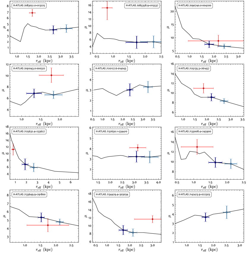
Figure 4: Magnification profiles of the reconstructed sources. The magnification factor, $\mu$, is evaluated in steps of SNR in the SP, from two up to the maximum and shown as a function of the effective radius of the area defined by the SP pixels with SNR above the adopted steps. The squares mark the values of the magnification calculated for SNR$\,=3$ (outermost; light blue square) and SNR$\,=5$ (innermost; dark blue square). The red point is the magnification factor estimated by B13. We have placed it at a radius corresponding to $2\times r_{\rm half}$, as this is the radius of the region in the SP used by B13 to compute the magnification. For HATLASJ142313.9+022303, the point of B13 is located outside the plotted region, at $r_{\rm eff}\sim 7\,$kpc.

4.1 Lens parameters

Fig. 3 compares our estimates of the lens mass model parameters with those of B13. In general we find good agreement, although there are some exceptions (e.g. HATLASJ133008.4+245900), particularly when multiple lenses are involved in the modelling, i.e. for HATLASJ083051.0+013225 and HATLASJ142413.9+022303. We briefly discuss each case individually.

HATLASJ083051.0+013225: This is a relatively complex system (see Fig. 1 of N17), with two foreground objects at different redshifts (B17) revealed at 1.1 $\micron$ and 2.2 $\micron$ by observations with HST/WFC3 (N17; Negrello et al. in prep.) and Keck/AO (Calanog et al., 2014), respectively. However the same data show some elongated structure north of the two lenses, which may be associated with the background galaxy, although this is still unclear due to the apparent lack of counter-images (a detailed lens modelling of this system performed on ALMA+HST+Keck data is currently ongoing; Negrello et al. in prep.). In our modelling we have assumed that the two lenses are at the same redshift, consistently with the treatment by B13. However, compared to B13, we derive an Einstein radius that is higher for one lens ($0.57^{\prime\prime}$ versus $0.43^{\prime\prime}$) and lower for the other one ($0.31^{\prime\prime}$ versus $0.39^{\prime\prime}$). The discrepancy is likely due to the complexity of the system, which may induce degeneracies among the model parameters; however it is worth mentioning that while we keep the position of both lenses as free parameters, B13 fixed the position of the second lens with respect to the first one, by setting the separation between the two foreground objects equal to that measured in the near-IR image.

HATLASJ085358.9+015537: This system was observed with Keck/NIRC2 in the $K_{s}$-band (Calanog et al., 2014). The background galaxy is detected in the near-IR in the form of a ring-like structure that was modelled by Calanog et al. assuming a SIE model for the lens and a Sérsic profile for the background source surface brightness. Our modelling of the SMA data gives results for the lens mass model consistent with those of Calanog et al., both indicating an almost spherical lens. B13 also find a nearly spherical lens ($q_{\rm L}\sim 0.94$) but with a different rotation angle ($\theta_{\rm L}\sim 160^{\circ}$ versus $\theta_{\rm L}\sim 62^{\circ}$), even though the discrepance is less than 3$\sigma$ once considered the higher confidence interval consequence of a spherical lens.

HATLASJ090740.0$-$004200: This is one of the first five lensed galaxies discovered in H-ATLAS (Negrello et al., 2010), and is also known as SDP.9. High-resolution observations at different wavelengths are available for this system, from the near-IR with HST/WFC3 (Negrello et al., 2014), to sub-mm with NOEMA (Oteo et al., 2017a) or 1.1mm with ALMA (Wong et al., 2017), to the X-ray band with Chandra (Massardi et al., 2017). The results of our lens modelling of the SMA data are consistent with those obtained by other groups at different wavelengths (Dye et al., 2014; Massardi et al., 2017, e.g.). However, B13 found a significantly lower lens axis-ratio compared to our estimate ($q_{\rm L}=0.50$ versus $q_{\rm L}=0.75$).

HATLASJ091043.1$-$000321: This is SDP.11, another of the first lensed galaxies discovered in H-ATLAS (Negrello et al., 2010). HST/WFC3 imaging data at 1.1$\micron$ reveals an elongated Einstein ring (Negrello et al., 2014), hinting to the effect of an external shear possibly associated with a nearby edge-on galaxy. In fact, Dye et al. (2014) introduced an external shear in their lens modelling of this system, which they constrained to have strength $\gamma\sim 0.23$. We also account for an external shear in our analysis. Our results are consistent with those of Dye et al. They also agree with the Einstein radius estimated by B13, although our lens is significantly more elongated and has a higher rotation angle. It is worth noticing, though, that B13 does not introduce an external shear in their analysis, which may explain the difference in the derived lens axial ratio.

HATLASJ120127.5$-$014043: This is the H-ATLAS source that we have confirmed to be lensed with the new SMA data. It is the only object in our sample for which we still lack a spectroscopic measure of the redshift of the background galaxy. The redshift estimated from the Herschel/SPIRE photometry is $z_{\rm sub-mm}=3.80\pm 0.58$. The reconstructed source is resolved into two knots of emission, separated by $\sim 3.5\,$kpc.

HATLASJ125135.4+261457: The estimated Einstein radius is slightly higher than reported by B13 ($\theta_{\rm E}=1.10\pm 0.02^{\prime\prime}$ versus $\theta_{\rm E}=1.02\pm 0.03^{\prime\prime}$) while the rotation angle of the lens is smaller ($\theta_{\rm L}=28\pm 2.5^{\circ}$ versus $\theta_{\rm L}=38\pm 1^{\circ}$). The reconstructed source is quite elongated, extending in the SW to NE direction, with a shape that deviates from a perfect ellipse. This might suggest that, at the scale probed by the SMA observations, the source comprises two partially blended components. This morphology is not accounted for by a single elliptical Sérsic profile, which may explain the observed discrepancies with the results of B13.

HATLASJ125632.7+233625: For this system we find a lens that is more elongated compared to the value derived by B13 ($q_{\rm L}=0.54\pm 0.09$ versus $q_{\rm L}=0.69\pm 0.03$). The reconstructed source morphology has a triangular shape which may bias the results on the lens parameters when the modelling is performed under the assumption of a single elliptical Sérsic profile, as in B13.

HATLASJ132630.1+334410: The background galaxy is lensed into two images, separated by $\sim 3.5^{\prime\prime}$, none of them resembling an arc. This suggests that the source is not lying on top of the tangential caustic, but away from it, although still inside the radial caustic to account for the presence of two images. As revealed by HST/WFC3 observations (see N17, their Fig. 3), the lens is located close to the southernmost lensed image. The lack of extended structures, like arcs or rings, makes the lens modelling more prone to degeneracies. Despite that, we find a good agreement with the results of B13.

HATLASJ133008.4+245900: Besides the lens modelling performed by B13 on SMA data, this system was also analysed by Calanog et al. (2014) using Keck/AO $K_{s}$-band observations, where the background galaxy is detected. The configuration of the multiple images is similar in the near-IR and in the sub-mm suggesting that the stellar and dust emission are co-spatial. We derive an Einstein radius $\theta_{\rm E}=1.03^{\prime\prime}$, higher than B13’s result ($\theta_{\rm E}=0.88^{\prime\prime}$). Our estimate is instead in agreement with the finding of Calanog et al. (2014) and Negrello et al. (in prep.; based on HST/WFC3 imaging data). Interestingly, the reconstructed background source is very elongated. This is due to the presence of two partially blended knots of emission, a main one extending across the tangential caustic and a second, fainter one located just off the fold of the caustic. This is another example where the assumption that the source is represented by a single Sérsic profile, made by B13, is probably affecting the estimated lens model parameters.

HATLASJ133649.9+291801: This is the single-lens system in our sample with the smallest Einstein radius, $\theta_{\rm E}=0.4^{\prime\prime}$. Our lens modelling gives results consistent with those of B13.

HATLASJ134429.4+303036: This is the 500$\,\mu$m brightest lensed galaxy in the entire N17 sample. The observed lensed images indicate a typical cusp configuration, similar to what was observed in the well studied lensed galaxy SDP.81 (e.g. Dye et al., 2015), where the background galaxy lies on the fold of the tangential caustic. According to our modelling the lens is significantly elongated ($q_{\rm L}=0.53$) in the North-South direction, consistent with what is indicated by available HST/WFC3 imaging data for the light distribution of the foreground galaxy (see Fig. 3 of N17). We estimate a higher Einstein radius than the one reported by B13, although the two results are still consistent within 2$\sigma$.

HATLASJ142413.9+022303: This source $-$ a 500$\,\mu$m “riser” $-$ was first presented in Cox et al. (2011) while the lens modelling, based on SMA data, was performed in Bussmann et al. (2012). Observations carried out with HST/WFC3 and Keck/AO (Calanog et al., 2014) revealed two foreground galaxies, separated by $\sim 0.3^{\prime\prime}$, although only one currently has a spectroscopic redshift, $z=0.595$ (B13). No emission from the background galaxy is detected in the near-IR. B13 modelled the system using two SIE profiles. We attempted the same but found no significant improvement in the results compared to the case of a single SIE mass distribution, which we have adopted here. We find $\theta_{\rm E}=0.97^{\prime\prime}$, consistent with the value derived from the lens modelling of ALMA data performed by Dye et al. (2017), which also assumed a single SIE profile. On the other hand B13 obtained $\theta_{\rm E,1}=0.57^{\prime\prime}$ and $\theta_{\rm E,2}=0.40^{\prime\prime}$ for the two lenses. In this case the comparison with the B13 results is not straightforward. It is also important to note, as shown in Fig. 2 [see also Dye et al. (2017)], that the background source has a complex extended morphology, which cannot be recovered by a single Sérsic profile. Bussmann et al. (2012) modelled this system assuming two Sérsic profiles for the background galaxy but their results, particularly for the position of the second knot of emission in the SP, disagree with ours and with the findings of Dye et al. (2017).

According to our findings, in single-lens systems the use of an analytic model for the source surface brightness does not bias the results on the SIE lens parameters as long as the background galaxy is not partially resolved into multiple knots of emission. A way to overcome this problem would be to test the robustness of the results by adding a second source during the fitting procedure. However, the drawback of this approach is the increase in the number of free parameters, and, therefore, the increased risk of degeneracies in the final solution. We conceived our SLI method to overcome this problem and we recommend it in the modelling of lensed galaxies.

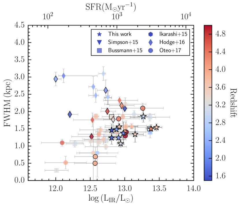
Figure 5: FWHMs of the sources in our sample (stars) as a function of their infrared luminosity, compared to results from literature: Simpson et al. (2015, triangle), Bussmann et al. (2015, squares), Ikarashi et al. (2015, hexagons), Hodge et al. (2016, diamonds), Oteo et al. (2017b, circles). All the sources taken from literature were fitted or (for the lensed ones) modelled using Gaussians and here we report, as an effective radius, the geometric mean of the values of the FWHM along the minor and the major axis. The only exception is the point of Simpson et al. which represents the median of the FWHM_major values for their sample (see Section 4.2). The data points are colored according to their redshift. Most objects have a photometric redshift estimate; those with a spectroscopic redshift measurement are highlighted by a dense black outline.

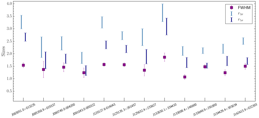
Figure 6: Comparison between the measured $5\sigma$ and $3\sigma$ effective radius and the geometric mean of the values of the FWHM along the minor and the major axis obtained from a Gaussian fit to the reconstructed source plane. The FWHMs are systematically lower then the reported effective radii obtained over a certain value of signal-to-noise value, due to lost features not retrieved by the Gaussian fit.

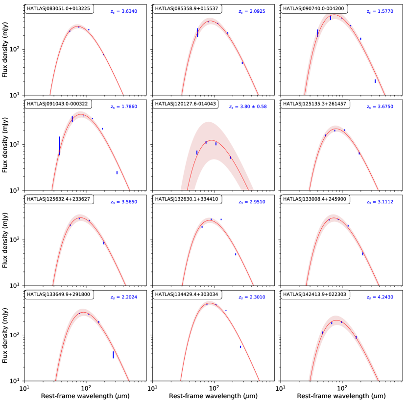
Figure 7: Observed far-IR to sub-mm SEDs of the 12 sources (blue error bars; from Herschel and SMA) together with the best-fitting modified black-body spectrum (red curve; assuming dust emissivity index $\beta=1.5$). The shaded red area shows the 68% confidence region associated with the best-fitting model. The redshift of the source is reported on the top-right corner of each panel. The redshift is spectroscopic for all the sources but one, i.e. HATLAS J120127.6-014043. This accounts for the significantly larger uncertainity in the fit to the SED of HATLAS J120127.6-014043 compared to the other sources.

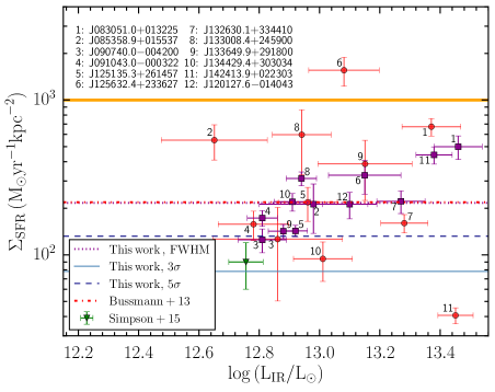
Figure 8: Star formation rate surface density as a function of infrared luminosity for the sources in our sample. The dark magenta squares correspond to the case $\mu=\mu_{5\sigma}$ and $A_{\rm dust}=A_{\rm dust,\,FWHM}$. The dotted dark magenta line marks their median value. The median value of $\Sigma_{\rm SFR}$ for the case $\mu=\mu_{5\sigma}$ and $A_{\rm dust}=A_{\rm dust,5\sigma}$ is shown by the dotted blue line, while the case of $\mu=\mu_{3\sigma}$ and $A_{\rm dust}=A_{\rm dust,3\sigma}$ is the continuous cyan line. For comparison we show the data points from B13 (red dots; calculated as explained in Section 4.3) and the median value of the SFR surface density of DSFGs from the Simpson et al. (2015) sample (green triangle). The yellow line marks the Eddington limit for a radiation pressure supported starburst galaxy (Thompson et al., 2005; Andrews & Thompson, 2011).

Table 4: Intrinsic properties of the 12 sources in our sample. The correction for the effect of lensing has been implemented by using the value $\mu=\mu_{3\sigma}$ for the magnification as reported in Table 3.
The dust temperature, ${\rm T}_{\rm dust}$, and the dust luminosities, ${\rm L}_{\rm FIR}$ (integrated in the rest-frame wavelength range $40-120\,\mu$m) and ${\rm L}_{\rm IR}$ (integrated over $8-1000\,\mu$m in the rest-frame), are derived by fitting the Herschel and SMA photometry with a modified blackbody spectrum with dust emissivity index $\beta=1.5$, as in Bussmann et al. (2013). Star formation rates, SFR, are estimated from ${\rm L}_{\rm IR}$ following Kennicutt & Evans (2012). The dust luminosity and SFR densities are computed as $\Sigma_{\rm FIR}={\rm L}_{\rm FIR}/A_{\rm dust,3\sigma}$, $\Sigma_{\rm IR}={\rm L}_{\rm IR}/A_{\rm dust,3\sigma}$ and $\Sigma_{\rm SFR}={\rm SFR}/A_{\rm dust,3\sigma}$, with the values of $A_{\rm dust,3\sigma}$ taken from Table 3.

IAUname	${\rm T}_{\rm dust}$	$\log{{\rm L}_{\rm FIR}}$	$\log{{\rm L}_{\rm IR}}$	SFR	$\log{\Sigma_{\rm FIR}}$	$\log{\Sigma_{\rm IR}}$	$\Sigma_{\rm SFR}$
	K	(${\rm L}_{\sun}$)	(${\rm L}_{\sun}$)	(${\rm M}_{\sun}{\rm yr}^{-1}$)	(${\rm L}_{\sun}$ kpc-2)	(${\rm L}_{\sun}$ kpc-2)	(${\rm M}_{\sun}{\rm yr}^{-1}$ kpc-2)
HATLASJ083051.0+013225	44.4$\pm$0.6	13.15$\pm$0.08	13.44$\pm$0.08	3540$\pm$560	11.63$\pm$0.08	11.91$\pm$0.08	105$\pm$25
HATLASJ085358.9+015537	37.4$\pm$0.7	12.94$\pm$0.17	12.97$\pm$0.17	1220$\pm$400	11.73$\pm$0.16	11.77$\pm$0.16	75$\pm$34
HATLASJ090740.0$-$004200	43.9$\pm$1.2	12.60$\pm$0.06	12.86$\pm$0.06	940$\pm$130	11.34$\pm$0.08	11.59$\pm$0.08	51$\pm$11
HATLASJ091043.1$-$000321	39.4$\pm$0.9	12.73$\pm$0.05	12.82$\pm$0.05	860$\pm$90	11.71$\pm$0.13	11.80$\pm$0.13	81$\pm$22
HATLASJ120127.6$-$014043	35.9$\pm$3.9	13.07$\pm$0.08	13.07$\pm$0.08	1530$\pm$260	11.55$\pm$0.07	11.55$\pm$0.07	46$\pm$10
HATLASJ125135.4+261457	41.2$\pm$0.7	12.81$\pm$0.03	12.96$\pm$0.03	1190$\pm$80	11.45$\pm$0.06	11.60$\pm$0.06	51$\pm$7
HATLASJ125632.7+233625	40.0$\pm$0.6	13.11$\pm$0.11	13.22$\pm$0.11	2140$\pm$470	11.76$\pm$0.13	11.87$\pm$0.13	96$\pm$32
HATLASJ132630.1+334410	38.6$\pm$0.6	13.21$\pm$0.09	13.27$\pm$0.09	2440$\pm$430	11.59$\pm$0.10	11.65$\pm$0.10	59$\pm$16
HATLASJ133008.4+245900	44.4$\pm$0.8	12.66$\pm$0.05	12.95$\pm$0.05	1150$\pm$120	11.52$\pm$0.07	11.80$\pm$0.07	82$\pm$15
HATLASJ133649.9+291801	36.0$\pm$0.7	12.93$\pm$0.03	12.93$\pm$0.03	1090$\pm$80	11.78$\pm$0.05	11.77$\pm$0.05	77$\pm$11
HATLASJ134429.4+303036	38.1$\pm$0.4	12.89$\pm$0.05	12.94$\pm$0.05	1140$\pm$130	11.73$\pm$0.08	11.79$\pm$0.08	80$\pm$16
HATLASJ142413.9+022303	39.6$\pm$1.0	13.20$\pm$0.08	13.32$\pm$0.08	2740$\pm$450	11.91$\pm$0.06	12.03$\pm$0.06	139$\pm$28

Table 5: Same as in Table 4, but this time assuming $\mu=\mu_{5\sigma}$ and $A_{\rm dust}=A_{\rm dust,5\sigma}$. The dust temperature is not listed here because it does not depend on the magnification, unless differential magnification is affecting the far-IR to sub-mm photometry.

IAUname	$\log{{\rm L}_{\rm FIR}}$	$\log{{\rm L}_{\rm IR}}$	SFR	$\log{\Sigma_{\rm FIR}}$	$\log{\Sigma_{\rm IR}}$	$\Sigma_{\rm SFR}$
	(${\rm L}_{\sun}$)	(${\rm L}_{\sun}$)	(${\rm M}_{\sun}{\rm yr}^{-1}$)	(${\rm L}_{\sun}$ kpc-2)	(${\rm L}_{\sun}$ kpc-2)	(${\rm M}_{\sun}{\rm yr}^{-1}$ kpc-2)
HATLASJ083051.0+013225	13.17$\pm$0.08	13.46$\pm$0.08	3720$\pm$650	11.83$\pm$0.06	12.11$\pm$0.06	167$\pm$35
HATLASJ085358.9+015537	12.95$\pm$0.18	12.98$\pm$0.18	1250$\pm$430	11.98$\pm$0.21	12.01$\pm$0.21	132$\pm$69
HATLASJ090740.0$-$004200	12.56$\pm$0.08	12.81$\pm$0.08	840$\pm$150	11.55$\pm$0.09	11.80$\pm$0.09	82$\pm$22
HATLASJ091043.1$-$000321	12.72$\pm$0.05	12.81$\pm$0.05	840$\pm$100	11.98$\pm$0.15	12.07$\pm$0.15	152$\pm$48
HATLASJ120127.6$-$014043	13.12$\pm$0.09	13.10$\pm$0.09	1650$\pm$320	11.87$\pm$0.06	11.86$\pm$0.06	95$\pm$23
HATLASJ125135.4+261457	12.77$\pm$0.04	12.92$\pm$0.04	1090$\pm$90	11.60$\pm$0.07	11.75$\pm$0.07	72$\pm$12
HATLASJ125632.7+233625	13.04$\pm$0.12	13.15$\pm$0.12	1840$\pm$450	12.00$\pm$0.16	12.11$\pm$0.16	166$\pm$65
HATLASJ132630.1+334410	13.20$\pm$0.08	13.27$\pm$0.08	2410$\pm$400	11.73$\pm$0.10	11.79$\pm$0.10	81$\pm$21
HATLASJ133008.4+245900	12.65$\pm$0.05	12.94$\pm$0.05	1120$\pm$110	11.72$\pm$0.12	12.01$\pm$0.12	132$\pm$35
HATLASJ133649.9+291801	12.88$\pm$0.05	12.88$\pm$0.05	980$\pm$100	12.02$\pm$0.06	12.01$\pm$0.06	134$\pm$23
HATLASJ134429.4+303036	12.86$\pm$0.06	12.91$\pm$0.06	1060$\pm$140	11.90$\pm$0.09	11.95$\pm$0.09	116$\pm$27
HATLASJ142413.9+022303	13.26$\pm$0.06	13.38$\pm$0.06	3130$\pm$400	12.30$\pm$0.08	12.42$\pm$0.08	344$\pm$71

4.2 Source magnifications and sizes

Fig. 4 shows, for each source, how the value of the magnification varies with the size of the region in the SP, as defined by the SNR of the pixels and here expressed in terms of $r_{\rm eff}$. The values of $\mu_{3\sigma}$ and $\mu_{5\sigma}$ are shown at the corresponding effective radii (light and dark blue squares, respectively), together with the magnification factor estimated by B13 (red dots). The latter is placed at a radius $r_{\rm eff}=2\times r_{\rm half}$, where $r_{\rm half}$ is the mean half-light radius of the Sérsic profile used by B13 to model the source surface brightness. It is calculated as $r_{\rm half}=a_{\rm s}\sqrt{1-\epsilon}$, with $a_{\rm s}$ and $\epsilon$ being the half-light semi-major axis length and ellipticity of the Sérsic profile provided by B13. B13 computed the magnification factor for an elliptical aperture in the SP with semi-major axis length equal to $2\times a_{\rm s}$. It is easy to show that the area of this region is exactly equal to $\pi\times(2\times r_{\rm half})^{2}$.
In general we find lower values of the magnification factor compared to B13. Discrepancies are to be expected for systems like HATLASJ083051.0+013225 and HATLASJ142413.9+022303, where the best-fitting lens model parameters differ significantly from those of B13. However a similar explanation may be also applied to systems like HATLASJ085358.9+015537,HATLASJ091043.0$-$000322, and HATLAS134429.4+303034. In HATLAS125135.3+261457, HATLASJ125632.4+233626 and HATLASJ133008.4+245900 the reconstructed source morphology is indicative of the presence of two partially blended components. The complexity of the source is not recovered by a single Sérsic profile and a significant fraction of the source emission lies beyond the region defined by B13 to compute $\mu$. As a consequence their magnification factor is higher than our estimate. HATLASJ090740.0$-$004200, HATLASJ132630.1+334410 and HATLASJ133649.9+291800 are the only systems where our findings are quite consistent with those of B13 for both the source size and the magnification.

In Fig. 5 we show the effective radius of the dust emitting region in DSFGs at $1.5\,\lower 2.0pt\hbox{${<\atop\hbox{\raise 4.0pt\hbox{$\sim$}}}$}\,z\,\lower 2.0pt\hbox{${<\atop\hbox{\raise 4.0pt\hbox{$\sim$}}}$}\,5$ from the literature, as a function of their infrared luminosity ($L_{\rm IR}$, integrated over the rest-frame wavelength range $8-1000\,\mu$m). Most of these estimates are obtained from ALMA continuum observations by fitting an elliptical Gaussian model to the source surface brightness. The value of $r_{\rm eff}$ reported in the figure is the geometric mean of the values of the FWHM of the minor and major axis lengths, unless otherwise specified. We provide below a brief description of the source samples presented in Fig. 5.

Simpson et al. (2015) carried out ALMA follow-up observations at 870$\micron$, with $\sim 0.3^{\prime\prime}$ resolution, of 52 DSFGs selected from the SCUBA-2 Cosmology Legacy Survey (S2CLS). They provide the median value of the FWHM of the major axis for the sub-sample of 23 DSFGs detected at more than 10$\,\sigma$ in the ALMA maps: FWHM${}_{\rm major}=2.4\pm 0.2\,$kpc. The median infrared luminosity of the same sub-sample is $L_{\rm IR}=(5.7\pm 0.7)\times 10^{12}\,L_{\odot}$. These are the values we show in Fig. 5 (triangular symbols), bearing in mind that we have no information on the ellipticity of the sources to correct for. Therefore, when comparing with other data sets, the Simpson et al. point should be considered as an upper limit.

Bussmann et al. (2015) have presented ALMA 870$\,\mu$m imaging data, at 0.45^′′ resolution, of 29 DSFGs from the Herschel Multi-tiered Extragalactic Survey (HerMES; Oliver et al., 2012). The sample includes both lensed and unlensed objects. Lens modelling is carried out assuming an elliptical Gaussian. The un-lensed galaxies are also modelled with an elliptical Gaussian. Their results are shown in Fig. 5 (square symbols), with FWHM$=2\times r_{s}$, where $r_{s}$ is the geometric mean of the semi-axes, as reported in their Table 3. The infrared luminosity of the lensed sources have been corrected for the magnification. We only show the sources in their sample that are not resolved into multiple components as no redshift and infrared luminosity are available for the individual components. This reduces their sample to nine objects: eight strongly lensed and one un-lensed.

Ikarashi et al. (2015) have exploited ALMA 1.1$\,\mu$m continuum observations to measure the size of a sample of 13 AzTEC-selected DSFGs with $z_{\rm phot}\sim 3-6$ and $L_{\rm IR}\sim 2-6\times 10^{12}\,L_{\odot}$. They fit the data in the $uv$-plane assuming a symmetrical Gaussian. In Fig. 5 we show their findings as FWHM$=2\times R_{c,e}$ (hexagon symbols), where $R_{c,e}$ is the value they quote in their Table 1 for the half-width at half-maximum of the symmetric Gaussian profile. Their 1.1$\,\mu$m flux densities have been rescaled to 870$\,\mu$m by multiplying them by a factor 1.5 (see Oteo et al. 2017). For most of the sources in the Ikarashi et al. sample the redshift is loosely constrained, with only lower limits provided. Therefore we only consider here two sources in their sample with an accurate photometric redshift, i.e. ASXDF1100.027.1 and ASXDF1100.230.1.

Hodge et al. (2016) used high resolution ($0.16^{\prime\prime}$) ALMA 870$\micron$ continuum observations of a sample of 16 DSFGs with $1\,\lower 2.0pt\hbox{${<\atop\hbox{\raise 4.0pt\hbox{$\sim$}}}$}\,z\,\lower 2.0pt\hbox{${<\atop\hbox{\raise 4.0pt\hbox{$\sim$}}}$}\,5$ and $L_{\rm IR}\sim 4\times 10^{12}\,L_{\odot}$ from the LABOCA Extended Chandra Deep Field South (ECDFS) sub-mm survey (LESS; Karim et al., 2013; Hodge et al., 2013) to investigate their size and morphology. Their results are represented by the diamond symbols in Fig. 5.

Oteo et al. (2017b, 2016) have performed ALMA 870$\,\mu$m continuum observations, at $\sim 0.12^{\prime\prime}$ resolution, of 44 ultrared DSFGs (i.e. with Herschel/SPIRE colors: $F_{\rm 500\mu m}/F_{\rm 250\mu m}>1.5$ and $F_{\rm 500\mu m}/F_{\rm 350\mu m}>1$). They confirmed a significant number of lensed galaxies, which we do not consider here because no lens modelling results are available for them yet. We only consider un-lensed objects for which Oteo et al. provide a photometric or a spectroscopic redshift (Riechers et al., 2017; Fudamoto et al., 2017; Oteo et al., 2016). When a source is resolved into multiple components, each component is fitted individually and an estimate of the SFR (and, therefore, of ${\rm L}_{\rm IR}$) is provided based on the measured 870$\,\mu$m flux density. The circles in Fig. 5 show their findings.

In order to compare with the data from literature we also fit our reconstructed source surface brightness using an elliptical Gaussian model. The derived values of the FWHM along the major and the minor axis of the ellipse are reported in Table 3 together with their geometric mean FWHM${}_{\rm m}=\sqrt{{\rm FWHM_{maj}}\times{\rm FWHM_{min}}}$. However we warn the reader that the use of a single Gaussian profile to model the observed surface brightness of DSFGs could bias the inferred sizes because of the clumpy nature of these galaxies, as partially revealed by our SMA data. In fact, we find that the values of ${\rm FWHM_{\rm m}}$ are systematically lower than those of $r_{\rm eff,5\sigma}$ and $r_{\rm eff,3\sigma}$, as demonstrated in Fig.6.

With this caveat in mind, we show in Fig. 5 the size of the dust emitting region derived from the Gaussian fit to our reconstructed source surface brightness. The infrared luminosity, obtained from a fit to the observed spectral energy distribution (see Section 4.3 for details), has been corrected for lensing by assuming $\mu=\mu_{5\sigma}$.
In Fig. 5 the data points are coloured according to their redshift. Most of the objects have a photometric redshift estimate; those with a spectroscopic redshift are highlighted by a black outline. We observe a significant scatter in the distribution of the source sizes, particularly at the lowest luminosities, with values ranging from $\,\lower 2.0pt\hbox{${<\atop\hbox{\raise 4.0pt\hbox{$\sim$}}}$}\,0.5\,$kpc to $\,\lower 2.0pt\hbox{${>\atop\hbox{\raise 4.0pt\hbox{$\sim$}}}$}\,3\,$kpc. The lack of sources with $r_{\rm eff}\,\lower 2.0pt\hbox{${<\atop\hbox{\raise 4.0pt\hbox{$\sim$}}}$}\,1\,$ kpc at ${\rm L}_{\rm IR}\,\lower 2.0pt\hbox{${>\atop\hbox{\raise 4.0pt\hbox{$\sim$}}}$}\,10^{13}\,{\rm L}_{\sun}$ is possibly a physical effect. In fact, such luminous sources would have extreme values of the SFR surface brightness, and, therefore, would be quite rare. The absence of $z>3.5$ sources with $r_{\rm eff}\,\lower 2.0pt\hbox{${>\atop\hbox{\raise 4.0pt\hbox{$\sim$}}}$}\,1.5\,$kpc and ${\rm L}_{\rm IR}\,\lower 2.0pt\hbox{${<\atop\hbox{\raise 4.0pt\hbox{$\sim$}}}$}\,3\times 10^{12}\,{\rm L}_{\sun}$ is likely due to their lower surface brightness, which makes these objects difficult to resolve in high resolution imaging data. Based on these considerations it is challenging to draw any conclusion about the dependence of the size on either luminosity or redshift.

The sources in our sample have a median effective radius $r_{\rm eff,5\sigma}\sim 1.77\,$kpc, rising to $r_{\rm eff,3\sigma}\sim 2.46\,$kpc if we consider all the pixels in the SP with SNR $>3$, while the median FWHM of the Gaussian model is $\sim 1.47\,$kpc. These values are consistent with what observed for other DSFGs at similar, or even higher, redshifts.

4.3 Star formation rate surface densities

We derive the star formation rate, SFR, of the sources in our sample from the magnification-corrected IR luminosity, ${\rm L}_{\rm IR}$, using the Kennicutt & Evans (2012) relation:

$${\rm SFR}\,({\rm M}_{\sun}\,{\rm yr^{-1}})\sim 1.3\,\times\,10^{-10}\,{\rm L}_{\rm IR}\,({\rm L}_{\sun})$$ (16)

which assumes a Kroupa initial mass function (IMF). B13 provide an estimate of the total far-infrared (FIR) luminosity, ${\rm L}_{\rm FIR}$ (integrated over the rest-frame wavelength range $40-120\,\mu$m), of the sources in their sample by performing a fit to the measured Herschel/SPIRE and SMA photometry using a single temperature, optically thin, modified blackbody spectrum with dust emissivity index $\beta=1.5$. The normalization of the spectrum and the dust temperature, ${\rm T}_{\rm dust}$, were the only free parameters. We have repeated that exercise using the Herschel/SPIRE photometry from the latest release of the H-ATLAS catalogues (Valiante et al., 2016, Furlanetto et al. in prep.; as listed in N17, their Table 4), including also the Herschel/PACS photometric data points, where available. The fit is performed using a Monte Carlo approach outlined in N17, to account for uncertainities in the photometry and in the redshift when the latter is not spectroscopically measured, as in the case of HATLASJ120127.6$-$014043. The observed spectral energy distribution (SED) and the best-fitting model are shown in Fig. 7.

The inferred infrared luminosities and star formation rates are listed in Table 4 and they have been corrected for the effect of lensing by assuming $\mu=\mu_{3\sigma}$ (see Table 3). To directly compare with B13 we also report, in the same table, the magnification-corrected far-IR luminosity. Table 5 shows the same results but corrected assuming $\mu=\mu_{\rm 5\sigma}$. The dust temperature is not listed in that table because it does not depend on lensing, unless differential magnification is affecting the far-IR to sub-mm photometry, thus biasing the results of the SED fitting. Unfortunately we cannot test if this is the case with the current data.

In both Table 4 and Table 5 we report the dust luminosity and star formation rate surface densities, defined as $\Sigma_{\rm IR}={\rm L}_{\rm IR}/A_{\rm dust}$ and $\Sigma_{\rm SFR}={\rm SFR}/A_{\rm dust}$ respectively. Both are corrected for the magnification and computed using the value of $A_{\rm dust}$ corresponding to the adopted SNR threshold in the SP.

Fig. 8 shows the SFR surface density of the sources in our sample as a function of their infrared luminosity (squares). We find median values $\Sigma_{\rm SFR,FWHM}=215\pm 114\,M_{\odot}\,$yr^-1kpc^-2 (dark magenta line) inside the region of radius $r={\rm FWHM_{\rm m}}$, and $\Sigma_{\rm SFR,5\sigma}=132\pm 69\,M_{\odot}\,$yr^-1kpc^-2 (dashed blue line) and $\Sigma_{\rm SFR,3\sigma}\sim 78\pm 25\,M_{\odot}\,$yr^-1kpc^-2 (dotted cyan line) inside the regions in the source plane with ${\rm SNR\geq 5}$ and ${\rm SNR\geq 3}$, respectively. The red circles are the findings of B13 for the same sources. We have computed them by taking the FIR luminosity quoted by B13 and first converting it into ${\rm L}_{\rm IR}$ (by multiplying ${\rm L}_{\rm FIR}$ by a factor 1.9, as reported in B13) and then into SFR using Eq. (16). Then we have divided the SFR by the source area calculated as $A_{\rm dust}=\pi r_{\rm half}^{2}$. Finally we have divided the result by 2. In fact, by definition, the region within the circle of radius $r_{\rm half}$ contributes only half of the total luminosity (and therefore SFR) of the source. The median value of the SFR surface densities calculated in this way is $\Sigma_{\rm SFR}\sim 219\,M_{\odot}\,$yr^-1kpc^-2 (dot-dashed red line) which is similar to our estimate inside the region of radius FWHM, although the data points of B13 (red circles) display a much larger scatter than ours, and higher than our estimate inside the region defined with ${\rm SNR}$. It is notable that the SFR surface density calculated in this way $-$ although consistent with what done in other works (e.g. Simpson et al., 2015; Oteo et al., 2017c) $-$ is not representative of the galaxy as a whole, but only of the central region, where the emission is likely to be more concentrated. Therefore such an estimate should be taken as an upper limit for the SFR surface brightness of the whole galaxy. However we cannot exclude that individual star forming regions, resolved in higher resolution imaging data, may show significantly higher values of $\Sigma_{\rm SFR}$.

We also show, in the same figure, the median SFR surface density of DSFGs from the Simpson et al. (2015) sample (green triangle). They estimated $\Sigma_{\rm SFR}=90\pm 30\,M_{\odot}\,$yr^-1kpc^-2, assuming a Salpter IMF, which decreases to $\Sigma_{\rm SFR}\sim 67\,M_{\odot}\,$yr^-1kpc^-2 if we assume a Kroupa IMF as in Eq. (16). Their estimate of the SFR surface density is consistent with ours, although their sample has a lower infrared luminosity on average. However their way of calculating $\Sigma_{\rm SFR}$ is exactly the same we have adopted to draw the B13 data points in Fig. 8 and therefore it is affected by the same caveat discussed above.

The solid yellow line, at $\sim 1000\,M_{\odot}\,$yr^-1kpc^-2, marks the theoretical limit for the SFR surface density in a radiation pressure supported star forming galaxy (Thompson et al., 2005; Andrews & Thompson, 2011). None of our sources are close to that limit, at variance with what was found by B13. However we cannot exclude, as mentioned before, that individual star forming regions, not fully resolved by our current data, may reach the theoretical limit or even exceed it.

5 Conclusions

We have reassessed the lens modelling and source reconstruction performed by Bussmann et al. (2013) on the SMA observations of a sample of 11 lensed galaxies selected from the H-ATLAS. We have also presented new SMA observations of a further seven candidate lensed galaxies from the H-ATLAS sample which allowed us to confirm the lensing in at least one case, which we have included in the lens modelling.

Our lens modelling is based on the Regularized Semilinear Inversion method described in Warren & Dye (2003) and Nightingale & Dye (2015), modified to deal directly with the observed visibilities in the uv plane. This is a semi-parametric method, meaning that the source surface brightness counts are retrieved by pixelizing (or tesselating) both the observed image plane and the source plane. This differs from what done in B13, where the source was assumed to be described by a single Sérsic profile. In this way, we are able to retrieve the original source morphology, which, for these kind of sources, is usually clumpy.

As expected, when the reconstructed source does not display complex morphologies, our results for the lens mass model agree in general with those of B13. The only exceptions involve the modelling of multiple lens systems (just two in our sample), where degeneracies between model parameters are more likely to occur.

The adopted source reconstruction technique allows us to define a signal-to-noise ratio map in the source plane. We use it to more robustly define the area of the dust emitting region in the source plane and its corresponding magnification, while in B13, the source extension is an arbitrary factor of the half-light radius of the adopted Sérsic profile. We report the size of the reconstructed sources in our sample as the radius of a circle that encloses all the source plane pixels with ${\rm SNR}>5$ (or ${\rm SNR}>3$). However, for a more straightforward comparison with results in literature, we also quote the value of the FWHM obtained from a Gaussian fit to the reconstructed source plane. For almost 50 percent of our sample the estimated effective radii are larger than $2\times r_{\rm half}$, i.e. the radius of the region chosen by B13 to represent the source physical size when computing the magnification. As a consequence, we estimate, in general, lower magnification factors than those quoted in B13.

Once corrected for the magnification, our sources still retain very high star formation rates ${\rm SFR}\sim 900-3500\,M_{\odot}\,$yr^-1. With a median effective radius $r_{\rm eff,5\sigma}\sim 1.77\,$kpc ($r_{\rm eff,3\sigma}\sim 2.46$ kpc) and a median ${\rm FWHM}\sim 1.47\,$kpc, our sample has a median SFR surface density $\Sigma_{\rm SFR,5\sigma}\sim 132\,M_{\odot}\,$yr${}^{-1}\,$kpc^-2 ($\Sigma_{\rm SFR,3\sigma}\sim 78\,M_{\odot}\,$yr${}^{-1}\,$kpc^-2 or $\Sigma_{\rm SFR,FWHM}\sim 215\,M_{\odot}\,$yr${}^{-1}\,$kpc^-2 from the Gaussian fit). This is consistent with what is observed for other DSFGs at similar redshifts, but it is only a $\sim$10 percent of the limit achievable in a radiation pressure supported starburst galaxy.

References

- ALMA Partnership et al. (2015) ALMA Partnership et al., 2015, \hrefhttp://dx.doi.org/10.1088/2041-8205/808/1/L4 ApJL, \hrefhttp://adsabs.harvard.edu/abs/2015ApJ…808L…4A 808, L4
- Andrews & Thompson (2011) Andrews B. H., Thompson T. A., 2011, in Röllig M., Simon R., Ossenkopf V., Stutzki J., eds, EAS Publications Series Vol. 52, EAS Publications Series. pp 275–276 (\hrefhttp://arxiv.org/abs/1101.3577 arXiv:1101.3577), \hrefhttp://dx.doi.org/10.1051/eas/1152045 doi:10.1051/eas/1152045
- Barnabè et al. (2009) Barnabè M., Czoske O., Koopmans L. V. E., Treu T., Bolton A. S., Gavazzi R., 2009, \hrefhttp://dx.doi.org/10.1111/j.1365-2966.2009.14941.x MNRAS, \hrefhttp://adsabs.harvard.edu/abs/2009MNRAS.399…21B 399, 21
- Bolton et al. (2008) Bolton A. S., Burles S., Koopmans L. V. E., Treu T., Gavazzi R., Moustakas L. A., Wayth R., Schlegel D. J., 2008, \hrefhttp://dx.doi.org/10.1086/589327 ApJ, \hrefhttp://adsabs.harvard.edu/abs/2008ApJ…682..964B 682, 964
- Bussmann et al. (2012) Bussmann R. S., et al., 2012, \hrefhttp://dx.doi.org/10.1088/0004-637X/756/2/134 ApJ, \hrefhttp://adsabs.harvard.edu/abs/2012ApJ…756..134B 756, 134
- Bussmann et al. (2013) Bussmann R. S., et al., 2013, \hrefhttp://dx.doi.org/10.1088/0004-637X/779/1/25 ApJ, \hrefhttp://adsabs.harvard.edu/abs/2013ApJ…779…25B 779, 25
- Bussmann et al. (2015) Bussmann R. S., et al., 2015, \hrefhttp://dx.doi.org/10.1088/0004-637X/812/1/43 ApJ, \hrefhttp://adsabs.harvard.edu/abs/2015ApJ…812…43B 812, 43
- Cañameras et al. (2015) Cañameras R., et al., 2015, \hrefhttp://dx.doi.org/10.1051/0004-6361/201425128 A&A, \hrefhttp://adsabs.harvard.edu/abs/2015A
- Calanog et al. (2014) Calanog J. A., et al., 2014, \hrefhttp://dx.doi.org/10.1088/0004-637X/797/2/138 ApJ, \hrefhttp://adsabs.harvard.edu/abs/2014ApJ…797..138C 797, 138
- Carlstrom et al. (2011) Carlstrom J. E., et al., 2011, \hrefhttp://dx.doi.org/10.1086/659879 PASP, \hrefhttp://adsabs.harvard.edu/abs/2011PASP..123..568C 123, 568
- Cox et al. (2011) Cox P., et al., 2011, \hrefhttp://dx.doi.org/10.1088/0004-637X/740/2/63 ApJ, \hrefhttp://adsabs.harvard.edu/abs/2011ApJ…740…63C 740, 63
- Dye & Warren (2005) Dye S., Warren S. J., 2005, \hrefhttp://dx.doi.org/10.1086/428340 ApJ, \hrefhttp://adsabs.harvard.edu/abs/2005ApJ…623…31D 623, 31
- Dye et al. (2008) Dye S., Evans N. W., Belokurov V., Warren S. J., Hewett P., 2008, \hrefhttp://dx.doi.org/10.1111/j.1365-2966.2008.13401.x MNRAS, \hrefhttp://adsabs.harvard.edu/abs/2008MNRAS.388..384D 388, 384
- Dye et al. (2014) Dye S., et al., 2014, \hrefhttp://dx.doi.org/10.1093/mnras/stu305 MNRAS, \hrefhttp://adsabs.harvard.edu/abs/2014MNRAS.440.2013D 440, 2013
- Dye et al. (2015) Dye S., et al., 2015, \hrefhttp://dx.doi.org/10.1093/mnras/stv1442 MNRAS, \hrefhttp://adsabs.harvard.edu/abs/2015MNRAS.452.2258D 452, 2258
- Dye et al. (2017) Dye S., et al., 2017, preprint, \hrefhttp://adsabs.harvard.edu/abs/2017arXiv170505413D (\hrefhttp://arxiv.org/abs/1705.05413 arXiv:1705.05413)
- Eales et al. (2010) Eales S., et al., 2010, \hrefhttp://dx.doi.org/10.1086/653086 PASP, \hrefhttp://adsabs.harvard.edu/abs/2010PASP..122..499E 122, 499
- Edge et al. (2013) Edge A., Sutherland W., Kuijken K., Driver S., McMahon R., Eales S., Emerson J. P., 2013, The Messenger, \hrefhttp://adsabs.harvard.edu/abs/2013Msngr.154…32E 154, 32
- Falco et al. (1985) Falco E. E., Gorenstein M. V., Shapiro I. I., 1985, \hrefhttp://dx.doi.org/10.1086/184422 ApJL, \hrefhttp://adsabs.harvard.edu/abs/1985ApJ…289L…1F 289, L1
- Feroz & Hobson (2008) Feroz F., Hobson M. P., 2008, \hrefhttp://dx.doi.org/10.1111/j.1365-2966.2007.12353.x MNRAS, \hrefhttp://adsabs.harvard.edu/abs/2008MNRAS.384..449F 384, 449
- Feroz et al. (2009) Feroz F., Hobson M. P., Bridges M., 2009, \hrefhttp://dx.doi.org/10.1111/j.1365-2966.2009.14548.x MNRAS, \hrefhttp://adsabs.harvard.edu/abs/2009MNRAS.398.1601F 398, 1601
- Fudamoto et al. (2017) Fudamoto Y., et al., 2017, \hrefhttp://dx.doi.org/10.1093/mnras/stx1956 MNRAS, \hrefhttp://adsabs.harvard.edu/abs/2017MNRAS.472.2028F 472, 2028
- Harris et al. (2012) Harris A. I., et al., 2012, \hrefhttp://dx.doi.org/10.1088/0004-637X/752/2/152 ApJ, \hrefhttp://adsabs.harvard.edu/abs/2012ApJ…752..152H 752, 152
- Hatsukade et al. (2015) Hatsukade B., Tamura Y., Iono D., Matsuda Y., Hayashi M., Oguri M., 2015, \hrefhttp://dx.doi.org/10.1093/pasj/psv061 PASJ, \hrefhttp://adsabs.harvard.edu/abs/2015PASJ…67…93H 67, 93
- Hezaveh et al. (2016) Hezaveh Y. D., et al., 2016, \hrefhttp://dx.doi.org/10.3847/0004-637X/823/1/37 ApJ, \hrefhttp://adsabs.harvard.edu/abs/2016ApJ…823…37H 823, 37
- Hodge et al. (2013) Hodge J. A., et al., 2013, \hrefhttp://dx.doi.org/10.1088/0004-637X/768/1/91 ApJ, \hrefhttp://adsabs.harvard.edu/abs/2013ApJ…768…91H 768, 91
- Hodge et al. (2016) Hodge J. A., et al., 2016, \hrefhttp://dx.doi.org/10.3847/1538-4357/833/1/103 ApJ, \hrefhttp://adsabs.harvard.edu/abs/2016ApJ…833..103H 833, 103
- Ikarashi et al. (2015) Ikarashi S., et al., 2015, \hrefhttp://dx.doi.org/10.1088/0004-637X/810/2/133 ApJ, \hrefhttp://adsabs.harvard.edu/abs/2015ApJ…810..133I 810, 133
- Karim et al. (2013) Karim A., et al., 2013, \hrefhttp://dx.doi.org/10.1093/mnras/stt196 MNRAS, \hrefhttp://adsabs.harvard.edu/abs/2013MNRAS.432….2K 432, 2
- Kennicutt & Evans (2012) Kennicutt R. C., Evans N. J., 2012, \hrefhttp://dx.doi.org/10.1146/annurev-astro-081811-125610 ARAA, \hrefhttp://adsabs.harvard.edu/abs/2012ARA..26A..50..531K 50, 531
- Koopmans et al. (2006) Koopmans L. V. E., Treu T., Bolton A. S., Burles S., Moustakas L. A., 2006, \hrefhttp://dx.doi.org/10.1086/505696 ApJ, \hrefhttp://adsabs.harvard.edu/abs/2006ApJ…649..599K 649, 599
- Kormann et al. (1994) Kormann R., Schneider P., Bartelmann M., 1994, A&A, \hrefhttp://adsabs.harvard.edu/abs/1994A
- Kroupa (2001) Kroupa P., 2001, \hrefhttp://dx.doi.org/10.1046/j.1365-8711.2001.04022.x MNRAS, \hrefhttp://adsabs.harvard.edu/abs/2001MNRAS.322..231K 322, 231
- Lawrence et al. (2007) Lawrence A., et al., 2007, \hrefhttp://dx.doi.org/10.1111/j.1365-2966.2007.12040.x MNRAS, \hrefhttp://adsabs.harvard.edu/abs/2007MNRAS.379.1599L 379, 1599
- Lupu et al. (2012) Lupu R. E., et al., 2012, \hrefhttp://dx.doi.org/10.1088/0004-637X/757/2/135 ApJ, \hrefhttp://adsabs.harvard.edu/abs/2012ApJ…757..135L 757, 135
- Massardi et al. (2017) Massardi M., et al., 2017, preprint, \hrefhttp://adsabs.harvard.edu/abs/2017arXiv170910427M (\hrefhttp://arxiv.org/abs/1709.10427 arXiv:1709.10427)
- Nayyeri et al. (2016) Nayyeri H., et al., 2016, \hrefhttp://dx.doi.org/10.3847/0004-637X/823/1/17 ApJ, \hrefhttp://adsabs.harvard.edu/abs/2016ApJ…823…17N 823, 17
- Negrello et al. (2010) Negrello M., et al., 2010, \hrefhttp://dx.doi.org/10.1126/science.1193420 Science, \hrefhttp://adsabs.harvard.edu/abs/2010Sci…330..800N 330, 800
- Negrello et al. (2014) Negrello M., et al., 2014, \hrefhttp://dx.doi.org/10.1093/mnras/stu413 MNRAS, \hrefhttp://adsabs.harvard.edu/abs/2014MNRAS.440.1999N 440, 1999
- Negrello et al. (2017) Negrello M., et al., 2017, \hrefhttp://dx.doi.org/10.1093/mnras/stw2911 MNRAS, \hrefhttp://adsabs.harvard.edu/abs/2017MNRAS.465.3558N 465, 3558
- Nightingale & Dye (2015) Nightingale J. W., Dye S., 2015, \hrefhttp://dx.doi.org/10.1093/mnras/stv1455 MNRAS, \hrefhttp://adsabs.harvard.edu/abs/2015MNRAS.452.2940N 452, 2940
- Oliver et al. (2012) Oliver S. J., et al., 2012, \hrefhttp://dx.doi.org/10.1111/j.1365-2966.2012.20912.x MNRAS, \hrefhttp://adsabs.harvard.edu/abs/2012MNRAS.424.1614O 424, 1614
- Omont et al. (2011) Omont A., et al., 2011, \hrefhttp://dx.doi.org/10.1051/0004-6361/201116921 A&A, \hrefhttp://adsabs.harvard.edu/abs/2011A
- Omont et al. (2013) Omont A., et al., 2013, \hrefhttp://dx.doi.org/10.1051/0004-6361/201220811 A&A, \hrefhttp://adsabs.harvard.edu/abs/2013A
- Oteo et al. (2016) Oteo I., et al., 2016, \hrefhttp://dx.doi.org/10.3847/0004-637X/827/1/34 ApJ, \hrefhttp://adsabs.harvard.edu/abs/2016ApJ…827…34O 827, 34
- Oteo et al. (2017a) Oteo I., et al., 2017a, preprint, \hrefhttp://adsabs.harvard.edu/abs/2017arXiv170105901O (\hrefhttp://arxiv.org/abs/1701.05901 arXiv:1701.05901)
- Oteo et al. (2017b) Oteo I., et al., 2017b, preprint, \hrefhttp://adsabs.harvard.edu/abs/2017arXiv170904191O (\hrefhttp://arxiv.org/abs/1709.04191 arXiv:1709.04191)
- Oteo et al. (2017c) Oteo I., Zwaan M. A., Ivison R. J., Smail I., Biggs A. D., 2017c, \hrefhttp://dx.doi.org/10.3847/1538-4357/aa5da4 ApJ, \hrefhttp://adsabs.harvard.edu/abs/2017ApJ…837..182O 837, 182
- Pilbratt et al. (2010) Pilbratt G. L., et al., 2010, A&A, 518, L1
- Planck Collaboration et al. (2014) Planck Collaboration et al., 2014, A&A, 571, A16
- Planck Collaboration et al. (2015) Planck Collaboration et al., 2015, \hrefhttp://dx.doi.org/10.1051/0004-6361/201424790 A&A, \hrefhttp://adsabs.harvard.edu/abs/2015A
- Riechers et al. (2017) Riechers D. A., et al., 2017, preprint, \hrefhttp://adsabs.harvard.edu/abs/2017arXiv170509660R (\hrefhttp://arxiv.org/abs/1705.09660 arXiv:1705.09660)
- Rybak et al. (2015) Rybak M., McKean J. P., Vegetti S., Andreani P., White S. D. M., 2015, \hrefhttp://dx.doi.org/10.1093/mnrasl/slv058 MNRAS, \hrefhttp://adsabs.harvard.edu/abs/2015MNRAS.451L..40R 451, L40
- Schneider & Sluse (2013) Schneider P., Sluse D., 2013, \hrefhttp://dx.doi.org/10.1051/0004-6361/201321882 A&A, \hrefhttp://adsabs.harvard.edu/abs/2013A
- Schneider & Sluse (2014) Schneider P., Sluse D., 2014, \hrefhttp://dx.doi.org/10.1051/0004-6361/201322106 A&A, \hrefhttp://adsabs.harvard.edu/abs/2014A
- Simpson et al. (2015) Simpson J. M., et al., 2015, \hrefhttp://dx.doi.org/10.1088/0004-637X/807/2/128 ApJ, \hrefhttp://adsabs.harvard.edu/abs/2015ApJ…807..128S 807, 128
- Skilling (2006) Skilling J., 2006, \hrefhttp://dx.doi.org/10.1214/06-BA127 Bayesian Anal., 1, 833
- Spilker et al. (2016) Spilker J. S., et al., 2016, \hrefhttp://dx.doi.org/10.3847/0004-637X/826/2/112 ApJ, \hrefhttp://adsabs.harvard.edu/abs/2016ApJ…826..112S 826, 112
- Suyu et al. (2006) Suyu S. H., Marshall P. J., Hobson M. P., Blandford R. D., 2006, \hrefhttp://dx.doi.org/10.1111/j.1365-2966.2006.10733.x MNRAS, \hrefhttp://adsabs.harvard.edu/abs/2006MNRAS.371..983S 371, 983
- Swinbank et al. (2010) Swinbank A. M., et al., 2010, \hrefhttp://dx.doi.org/10.1038/nature08880 Nature, \hrefhttp://adsabs.harvard.edu/abs/2010Natur.464..733S 464, 733
- Swinbank et al. (2011) Swinbank A. M., et al., 2011, \hrefhttp://dx.doi.org/10.1088/0004-637X/742/1/11 ApJ, \hrefhttp://adsabs.harvard.edu/abs/2011ApJ…742…11S 742, 11
- Swinbank et al. (2015) Swinbank A. M., et al., 2015, \hrefhttp://dx.doi.org/10.1088/2041-8205/806/1/L17 ApJL, \hrefhttp://adsabs.harvard.edu/abs/2015ApJ…806L..17S 806, L17
- Tamura et al. (2015) Tamura Y., Oguri M., Iono D., Hatsukade B., Matsuda Y., Hayashi M., 2015, \hrefhttp://dx.doi.org/10.1093/pasj/psv040 PASJ, \hrefhttp://adsabs.harvard.edu/abs/2015PASJ…67…72T 67, 72
- Thompson et al. (2005) Thompson T. A., Quataert E., Murray N., 2005, \hrefhttp://dx.doi.org/10.1086/431923 ApJ, \hrefhttp://adsabs.harvard.edu/abs/2005ApJ…630..167T 630, 167
- Treu & Koopmans (2004) Treu T., Koopmans L. V. E., 2004, \hrefhttp://dx.doi.org/10.1086/422245 ApJ, \hrefhttp://adsabs.harvard.edu/abs/2004ApJ…611..739T 611, 739
- Valiante et al. (2016) Valiante E., et al., 2016, \hrefhttp://dx.doi.org/10.1093/mnras/stw1806 MNRAS, \hrefhttp://adsabs.harvard.edu/abs/2016MNRAS.462.3146V 462, 3146
- Valtchanov et al. (2011) Valtchanov I., et al., 2011, \hrefhttp://dx.doi.org/10.1111/j.1365-2966.2011.18959.x MNRAS, \hrefhttp://adsabs.harvard.edu/abs/2011MNRAS.415.3473V 415, 3473
- Vegetti & Koopmans (2009) Vegetti S., Koopmans L. V. E., 2009, \hrefhttp://dx.doi.org/10.1111/j.1365-2966.2008.14005.x MNRAS, \hrefhttp://adsabs.harvard.edu/abs/2009MNRAS.392..945V 392, 945
- Vegetti et al. (2010) Vegetti S., Koopmans L. V. E., Bolton A., Treu T., Gavazzi R., 2010, \hrefhttp://dx.doi.org/10.1111/j.1365-2966.2010.16865.x MNRAS, \hrefhttp://adsabs.harvard.edu/abs/2010MNRAS.408.1969V 408, 1969
- Vieira et al. (2013) Vieira J. D., et al., 2013, \hrefhttp://dx.doi.org/10.1038/nature12001 Nature, \hrefhttp://adsabs.harvard.edu/abs/2013Natur.495..344V 495, 344
- Wallington et al. (1996) Wallington S., Kochanek C. S., Narayan R., 1996, \hrefhttp://dx.doi.org/10.1086/177401 ApJ, \hrefhttp://adsabs.harvard.edu/abs/1996ApJ…465…64W 465, 64
- Wardlow et al. (2013) Wardlow J. L., et al., 2013, \hrefhttp://dx.doi.org/10.1088/0004-637X/762/1/59 ApJ, \hrefhttp://adsabs.harvard.edu/abs/2013ApJ…762…59W 762, 59
- Warren & Dye (2003) Warren S. J., Dye S., 2003, \hrefhttp://dx.doi.org/10.1086/375132 ApJ, \hrefhttp://adsabs.harvard.edu/abs/2003ApJ…590..673W 590, 673
- Wong et al. (2017) Wong K. C., Ishida T., Tamura Y., Suyu S. H., Oguri M., Matsushita S., 2017, \hrefhttp://dx.doi.org/10.3847/2041-8213/aa7d4a ApJL, \hrefhttp://adsabs.harvard.edu/abs/2017ApJ…843L..35W 843, L35
- Yang et al. (2016) Yang C., et al., 2016, \hrefhttp://dx.doi.org/10.1051/0004-6361/201628160 A&A, \hrefhttp://adsabs.harvard.edu/abs/2016A
- de Jong et al. (2015) de Jong J. T. A., et al., 2015, \hrefhttp://dx.doi.org/10.1051/0004-6361/201526601 A&A, \hrefhttp://adsabs.harvard.edu/abs/2015A