Understanding Type Ia supernovae through their U-band spectra

Abstract

Context. Observations of Type Ia supernovae (SNe Ia) can be used to derive accurate cosmological distances through empirical standardization techniques. Despite this success neither the progenitors of SNe Ia nor the explosion process are fully understood. The U-band region has been less well observed for nearby SNe, due to technical challenges, but is the most readily accessible band for high-redshift SNe.

Aims. Using spectrophotometry from the Nearby Supernova Factory, we study the origin and extent of U-band spectroscopic variations in SNe Ia and explore consequences for their standardization and the potential for providing new insights into the explosion process.

Methods. We divide the U-band spectrum into four wavelength regions $\lambda($uNi$)$, $\lambda($uTi$)$, $\lambda($uSi$)$ and $\lambda($uCa$)$. Two of these span the Ca H&K $\lambda\lambda\leavevmode\nobreak\ 3934,3969$ complex. We employ spectral synthesis using SYNAPPS to associate the two bluer regions with Ni/Co and Ti.

Results. (1) The flux of the uTi feature is an extremely sensitive temperature/luminosity indicator, standardizing the SN peak luminosity to $0.116\pm 0.011$ mag RMS. A traditional SALT2.4 fit on the same sample yields a $0.135$ mag RMS. Standardization using uTi also reduces the difference in corrected magnitude between SNe originating from different host galaxy environments. (2) Early U-band spectra can be used to probe the Ni+Co distribution in the ejecta, thus offering a rare window into the source of lightcurve power. (3) The uCa flux further improves standardization, yielding a $0.086\pm 0.010$ mag RMS without the need to include an additional intrinsic dispersion to reach $\chi^{2}/\mathrm{dof}\sim 1$. This reduction in RMS is partially driven by an improved standardization of Shallow Silicon and 91T-like SNe.

1 Introduction

Type Ia supernovae (SNe Ia) are standardizable candles, and measuring their relative distances first led to the discovery of dark energy (Riess et al., 1998; Perlmutter et al., 1999). Their origin as thermonuclear explosions of CO WDs is well accepted, as is their importance as producers of heavy elements in the Universe (e.g. Maoz et al., 2014). It is further accepted that the light curve is powered by the decay of ⁵⁶Ni, which has a half-life of $\sim 6$ days for the dominant decay channel to Co. However, the progenitor system configuration and the path to detonation is still not understood. While a small sample of nearby SNe Ia now have tight limits on companions set by the lack of interaction or non-detection of hydrogen (Leonard, 2007; Bloom et al., 2012; Maguire et al., 2016), some SNe do show signs of H interaction (Hamuy et al., 2003; Aldering et al., 2006; Dilday et al., 2012) and theoretical explanations of the observed diversity prefer multiple explosion channels (Sim et al., 2013; Maeda & Terada, 2016).

Current lightcurve-based empirical SN Ia standardization methods yield a $\sim 0.1$ mag intrinsic dispersion (after accounting for measurement uncertainties), interpreted as a random scatter in magnitude and/or color (Betoule et al., 2014; Scolnic et al., 2014; Rubin et al., 2015). At least part of this observed scatter is due to differences in the explosion process, seen for example in a significantly reduced intrinsic dispersion when comparing spectroscopic twins (Fakhouri et al., 2015). These differences can, in turn, be expected to evolve differently with cosmic time and thus propagate into systematic limits on cosmological constraints from SNe Ia if left unresolved. Simultaneously, the origin of the peak-brightness correction for reddening is not fully understood, with lingering differences between empirical reddening curves and dust-like extinction in the U-band and between individual well-measured SNe (Guy et al., 2010; Chotard et al., 2011; Burns et al., 2014; Amanullah et al., 2015; Mandel et al., 2017; Huang et al., 2017). Evidence for an incomplete SN Ia standardization is also implied by the correlations between standardized magnitude and host-galaxy environment (Sullivan et al., 2010; Childress et al., 2013a; Rigault et al., 2013). Most recently, Rigault et al. (submitted, R17) have used the specific star formation rate measured at the projected SN location (local specific Star Formation Rate, LsSFR) to statistically classify individual SNe Ia as younger or older. Younger SNe Ia are found to be $0.16\pm 0.03$ mag fainter than older (after SALT2.4 standardization). The fraction of young SNe is expected to greatly increase as a function of redshift, an era where cosmology aims to be sensitive to slight deviations from the $\Lambda CDM$ model requires full understanding of all such effects.

Spectral features in the rest-frame U-band region ($\sim 3200$ to $4000$ Å) are less well explored compared with those at redder wavelengths. Empirical studies of U-band spectroscopic variability are few, and due to the atmosphere cutoff, usually dependent on high-$z$ or space-based data. Comparisons of samples at different redshifts have suggested an evolution of the mean U/UV properties (Ellis et al., 2008; Kessler et al., 2009; Foley et al., 2012; Milne et al., 2015). Foley et al. (2016) examined UV spectra of ten nearby SNe Ia obtained within five days of peak light, finding variations connected to optical lightcurve shape, and an increasing dispersion bluewards of $4000$ Å ($\lambda>4000$ Å). The Ca H&K $\lambda\leavevmode\nobreak\ 3945$ “feature”, dominated by Si ii $\lambda 3858$ and the Ca H&K $\lambda\lambda\leavevmode\nobreak\ 3934,3969$ doublet, is more frequently observed, but with conflicting interpretations. Maguire et al. (2012) and Foley (2013) find differences in EW(Ca H&K $\lambda 3945$) between samples divided by lightcurve width, but differ as to whether the Ca H&K $\lambda\leavevmode\nobreak\ 3945$ velocity correlates with lightcurve width. Foley et al. (2011) found high Ca ii velocity SNe to be intrinsically redder. High Velocity Features (HVFs) – absorption features that are detached from a “photospheric” component – have long been observed in early SNe Ia spectra (Mazzali et al., 2005; Tanaka et al., 2006), and potentially yield insights into the outer ejecta density or ionization (Blondin et al., 2013). Several studies have tried to systematically map the presence of detached HVFs in the Ca IR and H&K regions. Fitting coupled Gaussian functions to the Ca features, Childress et al. (2014) found that neither rapidly declining SNe nor SNe with high photospheric velocity show HVFs at peak light. Silverman et al. (2015) reached similar conclusions based on a larger sample.

Individual SNe with early U-band spectroscopy include PTF13asv, showing an initially suppressed U-band flux at day $-14$ that brightened significantly during the following five days (Cao et al., 2016), possibly due to an outer, thin region of radioactive material. PS1-10afx was first reported as a new transient type by Chornock et al. (2013), but later found to be a gravitationally magnified high-z SN Ia (Quimby et al., 2013, 2014). The spectral comparison of Chornock et al. (2013) (their Fig. 7) shows a brighter flux in the bluest part of the U-band, differing from comparison SNe Ia (SN2011fe, SN2011iv). The UV/U-band spectrum of SN2004dt is discussed in Wang et al. (2012), where low-resolution HST-ACS spectra show excess U-band flux close to peak. Further studies of individual SNe with U-band spectroscopic coverage have been presented for example by Patat et al. (1996); Garavini et al. (2004); Altavilla et al. (2007); Stanishev et al. (2007); Garavini et al. (2007); Matheson et al. (2008); Wang et al. (2009); Bufano et al. (2009); Blondin et al. (2012); Silverman et al. (2012); Wang et al. (2012); Smitka et al. (2015). Significant variation in flux for different phases of observation and between objects can be found, but due to uneven candidate and cadence selection this variability has proven hard to quantify.

The $3000$-$4000$ Å region is situated at the opacity transition region, going from fully dominated by Iron Group Element (IGE) line absorption in the UV to electron-scattering in the B-band, with the SN Spectral Energy Distribution (SED) shaped by a mix of IGE and Intermediate Mass Element (IME) features. Theoretical predictions of the U-band spectrum thus have to take both effects correctly into account (Pinto & Eastman, 2000), making it hard to gauge the level of systematic uncertainties on the U-band SED predictions from current models. Simulations have found progenitor metallicity to cause significant variations bluewards of the U-band wavelength region, but with few clear predictions within this region (Timmes et al., 2003; Walker et al., 2012).

Here we attempt to gain a deeper understanding of the U-band region, both to provide data for comparison with predictions from explosion scenarios and to improve the use of SNe Ia as standardizable candles. This will have particular implications for SNe at high-$z$, where restframe U-band observations are naturally obtained by ground-based imaging surveys and important for constraining the transient type (either at initial detection to trigger follow-up, or during a final photometry-only analysis).

The initial motivation for this study and the approach of dividing the U-band spectrum into four wavelength subregions arose from the comparison of individual supernovae having similar BVR spectra and lightcurve properties but exhibiting spectroscopic differences in the U-band. We present the sample and introduce this subdivision in Sec. 2, and study U-band spectroscopic variability in Sec. 3. Sec. 4 contains a discussion of how the SN Ia explosion can be examined using U-band absorption features. In Sec. 5 we explore the consequences for SN Ia standardization. Finally, in Sec. 6 we discuss the presence of SN Ia subclasses based on U-band flux measurements, return to the question of HVFs, and provide a brief outlook. We conclude in Sec. 7.

2 Data and U-band measurables

2.1 Nearby Supernova Factory

The Nearby Supernova Factory (SNfactory) has obtained time-series spectrophotometry of a large number of SNe Ia in the Hubble flow. Observations have been performed with our SuperNova Integral Field Spectrograph (SNIFS, Aldering et al., 2002; Lantz et al., 2004). SNIFS is a fully integrated instrument optimized for automated observation of point sources on a structured background over the full ground-based optical window at moderate spectral resolution ($R\sim 500$). It consists of a high throughput wide-band lenslet integral field spectrograph, a multi-filter photometric channel to image the field in the vicinity of the IFS for atmospheric transmission monitoring simultaneously with spectroscopy, and an acquisition/guiding channel. The IFS possesses a fully-filled $6.4\arcsec\times 6.4\arcsec$ spectroscopic field of view subdivided into a grid of $15\times 15$ spatial elements, a dual-channel spectrograph covering $3200-5200$ Å and $5100-10000$ Å simultaneously, and an internal calibration unit (continuum and arc lamps). SNIFS is mounted on the south bent Cassegrain port of the University of Hawaii $2.2$ m telescope on Mauna Kea, and is operated remotely. Observations are reduced using a dedicated data reduction pipeline, similar to that presented in §4 of Bacon et al. (2001). Discussion of the software pipeline is given in Aldering et al. (2006) and updated in Scalzo et al. (2010). Of particular importance for this analysis is the flux calibration and Mauna Kea atmosphere model presented in Buton et al. (2013). This provides accurate flux calibration down to $\sim 3300$ Å with a residual $\sim 2\%$ grey scatter. The extension to bluer wavelengths compared with most ground-based observations is a key prerequisite for this study. Host-galaxy subtraction is performed as described in Bongard et al. (2011), a methodology subsequently improved and made more flexible. Each spectrum is corrected for Milky Way dust extinction (Schlegel et al., 1998), blue-shifted to rest-frame based on the heliocentric host-galaxy redshift (Childress et al., 2013b, R17) and the fluxes are converted to luminosity assuming distances expected for the supernova redshifts in the CMB frame and assuming a dark energy equation of state $w=-1$. For the purpose of fitting LCs with SALT2.4 and calculating Hubble residuals, magnitudes are generated through integration over the following top-hat profiles: $\mathrm{U}_{\mathrm{SNf}}$ ($3300-4102$ Å), $\mathrm{B}_{\mathrm{SNf}}$ ($4102-5100$ Å), $\mathrm{V}_{\mathrm{SNf}}$ ($5200-6289$ Å), $\mathrm{R}_{\mathrm{SNf}}$ ($6289-7607$ Å) and $\mathrm{I}_{\mathrm{SNf}}$ ($7607-9200$ Å).

2.2 Sample

The sample is based on a slightly enlarged version of the data presented in previous SNfactory publications (Chotard et al., 2011; Rigault et al., 2013; Feindt et al., 2015; Fakhouri et al., 2015). We require all SNe to have a first high signal-to-noise spectrum prior to $-2$ days. We have updated SALT lightcurve fits to the latest version (SALT2.4, Betoule et al., 2014), and require these to provide a good fit to synthetic broadband photometry generated from the data (five failed this in a blinded inspection). $\mathrm{U}_{\mathrm{SNf}}$ photometry was not included in these fits since Saunders et al. (2015) demonstrated that the UV is not well described by the SALT2.4 model. Finally, four 91bg-like SNe were removed. The final sample consists of $92$ SNe Ia. Out of this set, $73$ SNe are found in the $0.03<z<0.1$ redshift range. Spectra shown below are cut redward of $\sim 6500$ Å for display purposes only.

Host-galaxy properties were presented in Childress et al. (2013a) and R17, where $z$, SALT2.4 $x_{1}$, $c$ and Hubble residuals have also been tabulated. Besides the frequently-used global stellar mass (Sullivan et al., 2010; Childress et al., 2013a), this includes the local specific star formation rate (LsSFR). The LsSFR combines the local $H\alpha$ flux (driven by UV-emission from young stars) with the estimated local stellar mass, thus producing an estimate for the fraction of young stars at the SN location. SNe with large LsSFR values are more likely to originate from a young progenitor, while SNe in low LsSFR environments likely originate from older systems. This provides refined information compared with earlier global measurements as star forming galaxies can have locally passive (old) regions. The lightcurve width, color and host-galaxy mass distributions of this sample closely match that of the combined SNLS and SDSS data in the JLA sample (Betoule et al., 2014).

Measurements of the equivalent width (EW) and velocity of the Si ii $\lambda 6355$ absorption feature were made on spectra within $\pm 2.5$ days from (B-band) maximum. These spectroscopic-indicator measurements are further described in Chotard (2011), and a spectroscopic-indicator analysis based on the full SNfactory sample will be presented in Chotard et al. (in prep.).

We focus on spectra in three restframe phase bins, pre-peak ($-8$ to $-4$ days with respect to B-band peak as determined by SALT2.4), peak ($-2$ to $2$ days) and post-peak ($4$ to $8$ days). This selection strikes a balance between capturing how quickly SNe Ia vary while limiting the number of new parameters to inspect. Spectra are dereddened based on the optical colors so that, to first order, intrinsic spectroscopic variations can be distinguished from extinction by dust. The correct color curve to apply, which could vary from object to object, is not fully understood. We further do not want to assume that intrinsic U-band features do not correlate with reddening, as these potentially could be indirectly caused by relations between intrinsic SN-features and the progenitor environment. In order to minimize the potential impact of systematic differences due to reddening, we take two conservative steps: (1) Remove reddened SNe with SALT2.4 color $c>0.2$ from further analysis and (2) make an initial dereddening correction assuming the extinction curve of Fitzpatrick (1999, F99) with $R=3.1$. Three SNe have $c>0.2$ and thus will not be included in the main analysis, unless otherwise noted. The $E(B-V)$ values used when dereddening are based on SALT2.4 $c$ measurements, derived from the $\mathrm{B}_{\mathrm{SNf}}\mathrm{V}_{\mathrm{SNf}}\mathrm{R}_{\mathrm{SNf}}$ bands, and converted to E$($B$-$V$)$ according to Eq. 6 of Guy et al. (2010). In Sec. 5.3 we will return to how this choice of method of accounting for reddening by dust influences measurements.

2.3 Definition of U-band indices

Here we examine SN2011fe and SNF20080514-002 as a sample pair of SNe with (relatively) similar $B_{\mathrm{SNf}}V_{\mathrm{SNf}}R_{\mathrm{SNf}}$ spectra and lightcurve properties, but large absorption feature differences in the U-band. Their early and peak spectra are compared in Fig. 1. Spectral differences between these objects can be localized to different behavior in four subdivisions of the U-band wavelength region: $\lambda($uNi$)$ ($3300$–$3510$ Å), $\lambda($uTi$)$ ($3510$–$3660$ Å), $\lambda($uSi$)$ ($3660$–$3750$ Å) and $\lambda($uCa$)$ ($3750$–$3860$ Å). The two redder regions, roughly covering the Ca H&K $\lambda\leavevmode\nobreak\ 3945$ feature, are dominated by Si ii $\lambda 3858$ & Ca H&K $\lambda\lambda\leavevmode\nobreak\ 3934,3969$ absorption. These wavelength regions are thus labeled $\lambda($uSi$)$ ($3660$–$3750$ Å) and $\lambda($uCa$)$ ($3750$–$3860$ Å). The blue half of the U-band is also divided into two parts. The left (early) panel of Fig. 1 shows differences up to $\sim 3500$ Å, a region labeled $\lambda($uNi$)$. The peak spectra (right panel of Fig. 1 agree in this region but differ in the subsequent $\sim 3500$ to $\sim 3700$ Å section, here denoted $\lambda($uTi$)$. The ions most frequently found to dominate these regions are used as labels, but it is clear that absorbing elements will vary with phase and between SNe (see Sec. 4.1 for further discussions). In particular, High Velocity Features dominate variations at early phases in the $\lambda($uTi$)$ and $\lambda($uSi$)$ regions, but have more limited effects at other times and regions (see Sec. 6.1.)

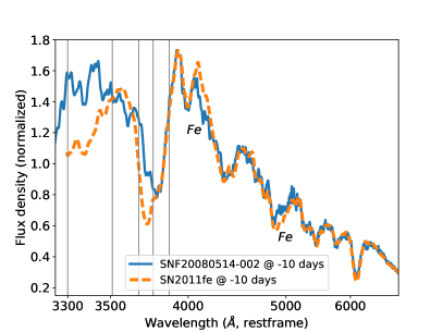
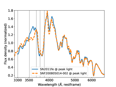
Figure 1: Comparison of the spectra of SN2011fe (SALT2.4 $x_{1}=-0.4$ and $c=-0.06$) and SNF200805014-002 (SALT2.4 $x_{1}=-1.5$ and $c=-0.12$) at early (left) and peak (right) phases. Small spectroscopic differences are found redwards of $4000$ Å (stable Fe marked in left panel). Much larger deviation is found bluewards of this limit. The comparison at early phases differs most strongly around $3400$ Å and the high velocity edge of the Ca H&K $\lambda\leavevmode\nobreak\ 3945$ feature, the comparison at later phases mainly around $3550$ Å. These differences led to the subdivision of the U-band into four indices, as described in the text. Vertical lines show the feature limits thus defined.

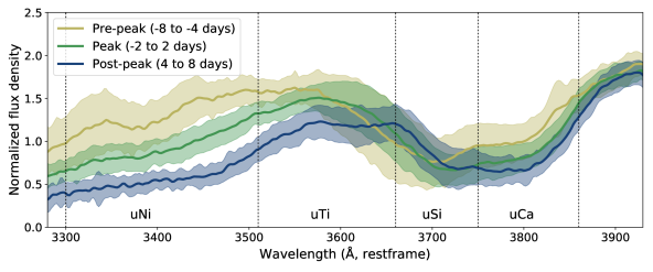
Figure 2: Mean spectra and $\pm 1$ standard deviation in sample at three representative phases. The four wavelength regions considered are separated by dashed lines. The interpretation of these indices will be phase dependent, as e.g. the Ti region at early phases is clearly a part of the Ca H&K $\lambda\leavevmode\nobreak\ 3945$ + Si ii $\lambda 3858$ feature complex and Cr/Fe dominates uNi at late phases.

We use the most straightforward and simple method to quantify U-feature variations – integration of flux within each wavelength region defined above, normalized by the $B_{\mathrm{SNf}}$-band flux at the same phase. We thus determine the spectral index uNi as

$$\mathrm{uNi}=-2.5\log\left(\frac{\int_{3300}^{3510}L_{dered}^{rest}(\lambda)d\lambda}{\int_{4102}^{5100}L_{dered}^{rest}(\lambda)d\lambda}\right).$$ (1)

The spectral indices uTi, uSi, and uCa are calculated in the same manner by simply changing the wavelength limits of the numerator. Each spectral index is thus a restframe, phase-dependent, dereddened color. For SNe with multiple spectra within a phase bin, measurements from these spectra are averaged, using the inverse variance from photon counting as weights. Within each phase bin we find weak dependencies with phase. For each feature/phase combination we fit a linear slope using the full sample and use this to correct individual measurements to the central bin phase ($-6$, $0$ or $6$ days).

Table 1: SN U-band properties and Ca High Velocity Feature classification.

Name	Phase $-8$ to $-4$				Phase $-2$ to $2$				Phase $4$ to $8$				Ca HVF
	uNi	uSi	uCa	uTi	uNi	uSi	uCa	uTi	uNi	uSi	uCa	uTi
SNF20050728-006	$1.76\pm 0.04$	$3.41\pm 0.04$	$2.53\pm 0.03$	$1.97\pm 0.04$	$2.04\pm 0.05$	$3.38\pm 0.06$	$2.77\pm 0.04$	$1.92\pm 0.04$	$2.62\pm 0.04$	$3.16\pm 0.03$	$3.00\pm 0.03$	$2.12\pm 0.03$	Y
SNF20050821-007	$2.00\pm 0.04$	$3.51\pm 0.04$	$2.29\pm 0.03$	$2.28\pm 0.04$	$2.32\pm 0.04$	$3.73\pm 0.04$	$2.50\pm 0.03$	$2.24\pm 0.04$	$2.61\pm 0.04$	$3.96\pm 0.04$	$2.70\pm 0.03$	$2.47\pm 0.04$	Y
SNF20051003-004	$1.57\pm 0.04$	$2.57\pm 0.03$	$2.44\pm 0.02$	$1.96\pm 0.03$	–	–	–	–	$2.65\pm 0.04$	$2.79\pm 0.03$	$2.90\pm 0.02$	$2.15\pm 0.03$	–
SNF20060512-001	$1.94\pm 0.04$	$2.71\pm 0.03$	$2.23\pm 0.02$	$1.76\pm 0.03$	$2.25\pm 0.04$	$2.76\pm 0.03$	$2.42\pm 0.02$	$1.78\pm 0.03$	$2.66\pm 0.04$	$2.97\pm 0.03$	$2.67\pm 0.02$	$2.01\pm 0.03$	Y
SNF20060526-003	$1.75\pm 0.04$	$3.03\pm 0.04$	$2.46\pm 0.03$	$2.09\pm 0.04$	$2.14\pm 0.04$	$3.04\pm 0.03$	$2.71\pm 0.03$	$2.01\pm 0.03$	–	–	–	–	Y
SNF20060609-002	–	–	–	–	$1.77\pm 0.04$	$2.69\pm 0.03$	$2.72\pm 0.03$	$1.89\pm 0.03$	$2.35\pm 0.04$	$2.73\pm 0.03$	$2.90\pm 0.03$	$2.09\pm 0.03$	–
SNF20060618-023	$1.32\pm 0.05$	$2.41\pm 0.05$	$2.15\pm 0.04$	$1.45\pm 0.04$	–	–	–	–	$2.48\pm 0.05$	$2.76\pm 0.04$	$2.76\pm 0.04$	$1.99\pm 0.04$	–
SNF20060621-015	$1.88\pm 0.04$	$3.02\pm 0.03$	$2.57\pm 0.02$	$1.91\pm 0.03$	$2.21\pm 0.04$	$3.00\pm 0.03$	$2.82\pm 0.02$	$1.95\pm 0.03$	$2.82\pm 0.04$	$2.96\pm 0.03$	$3.05\pm 0.03$	$2.24\pm 0.03$	N
SNF20060907-000	–	–	–	–	$2.24\pm 0.04$	$3.00\pm 0.03$	$2.88\pm 0.02$	$2.00\pm 0.03$	$2.98\pm 0.04$	$3.07\pm 0.03$	$3.13\pm 0.03$	$2.38\pm 0.03$	–
SNF20060916-002	$1.59\pm 0.04$	$2.87\pm 0.03$	$2.46\pm 0.03$	$2.00\pm 0.03$	–	–	–	–	$2.54\pm 0.04$	$2.89\pm 0.03$	$2.90\pm 0.03$	$2.17\pm 0.03$	N
SNF20061011-005	–	–	–	–	–	–	–	–	–	–	–	–	Y
SNF20061021-003	$1.67\pm 0.04$	$3.19\pm 0.03$	$2.66\pm 0.03$	$1.90\pm 0.03$	$2.05\pm 0.04$	$3.20\pm 0.03$	$2.94\pm 0.03$	$1.92\pm 0.03$	–	–	–	–	N
SNF20070330-024	$1.93\pm 0.04$	$3.20\pm 0.04$	$2.35\pm 0.03$	$2.36\pm 0.04$	$2.26\pm 0.04$	$3.34\pm 0.03$	$2.77\pm 0.03$	$2.16\pm 0.03$	$2.67\pm 0.04$	$3.15\pm 0.03$	$2.79\pm 0.02$	$2.21\pm 0.03$	–
SNF20070420-001	$1.67\pm 0.05$	$3.30\pm 0.06$	$2.42\pm 0.04$	$2.33\pm 0.05$	–	–	–	–	$2.82\pm 0.06$	$3.21\pm 0.05$	$2.90\pm 0.04$	$2.24\pm 0.04$	–
SNF20070424-003	$1.86\pm 0.04$	$3.42\pm 0.04$	$2.52\pm 0.03$	$2.09\pm 0.03$	$2.23\pm 0.05$	$3.23\pm 0.05$	$2.80\pm 0.04$	$2.06\pm 0.04$	$2.84\pm 0.06$	$3.04\pm 0.04$	$2.95\pm 0.04$	$2.34\pm 0.04$	Y
SNF20070506-006	$1.92\pm 0.04$	$2.79\pm 0.03$	$2.26\pm 0.02$	$1.82\pm 0.03$	$2.11\pm 0.04$	$2.88\pm 0.03$	$2.47\pm 0.02$	$1.85\pm 0.03$	$2.62\pm 0.04$	$3.15\pm 0.03$	$2.74\pm 0.02$	$2.10\pm 0.03$	–
SNF20070630-006	–	–	–	–	$2.07\pm 0.04$	$3.28\pm 0.04$	$2.73\pm 0.03$	$1.97\pm 0.03$	$2.66\pm 0.06$	$3.20\pm 0.05$	$2.94\pm 0.05$	$2.23\pm 0.04$	Y
SNF20070712-003	$1.75\pm 0.04$	$2.78\pm 0.03$	$2.63\pm 0.03$	$1.82\pm 0.03$	$2.16\pm 0.04$	$2.87\pm 0.03$	$2.87\pm 0.03$	$1.90\pm 0.03$	$2.72\pm 0.05$	$2.76\pm 0.03$	$3.08\pm 0.03$	$2.21\pm 0.03$	N
SNF20070717-003	$2.03\pm 0.05$	$3.50\pm 0.05$	$2.71\pm 0.03$	$2.01\pm 0.04$	$2.48\pm 0.07$	$3.20\pm 0.06$	$3.03\pm 0.06$	$2.17\pm 0.04$	$2.98\pm 0.07$	$3.10\pm 0.05$	$3.17\pm 0.05$	$2.38\pm 0.04$	N
SNF20070802-000	$1.68\pm 0.04$	$3.65\pm 0.03$	$2.40\pm 0.02$	$2.29\pm 0.03$	$2.09\pm 0.04$	$3.84\pm 0.04$	$2.72\pm 0.03$	$2.14\pm 0.03$	$2.60\pm 0.08$	$3.48\pm 0.08$	$2.87\pm 0.05$	$2.32\pm 0.05$	Y
SNF20070803-005	$1.53\pm 0.04$	$2.29\pm 0.03$	$2.10\pm 0.02$	$1.73\pm 0.03$	$2.02\pm 0.04$	$2.39\pm 0.03$	$2.27\pm 0.02$	$1.84\pm 0.03$	$2.64\pm 0.04$	$2.39\pm 0.03$	$2.45\pm 0.02$	$2.06\pm 0.03$	–
SNF20070810-004	$1.90\pm 0.04$	$3.75\pm 0.05$	$2.66\pm 0.03$	$2.01\pm 0.03$	–	–	–	–	$2.77\pm 0.05$	$3.37\pm 0.04$	$3.07\pm 0.04$	$2.28\pm 0.04$	N
SNF20070817-003	–	–	–	–	$2.29\pm 0.04$	$3.09\pm 0.03$	$2.79\pm 0.03$	$2.17\pm 0.03$	$3.17\pm 0.08$	$3.11\pm 0.05$	$3.04\pm 0.05$	$2.51\pm 0.04$	N
SNF20070818-001	–	–	–	–	$2.24\pm 0.06$	$3.59\pm 0.08$	$2.71\pm 0.04$	$2.30\pm 0.05$	$3.13\pm 0.15$	$3.42\pm 0.13$	$3.00\pm 0.10$	$2.47\pm 0.07$	–
SNF20070831-015	–	–	–	–	$2.17\pm 0.04$	$3.22\pm 0.03$	$2.48\pm 0.03$	$1.86\pm 0.03$	$2.58\pm 0.04$	$3.32\pm 0.04$	$2.64\pm 0.03$	$2.04\pm 0.03$	Y
SNF20070902-018	–	–	–	–	$2.18\pm 0.04$	$2.84\pm 0.03$	$2.82\pm 0.03$	$1.98\pm 0.03$	–	–	–	–	–
SNF20071003-004	–	–	–	–	–	–	–	–	$2.91\pm 0.07$	$3.28\pm 0.05$	$3.05\pm 0.04$	$2.27\pm 0.04$	–
SNF20071021-000	$1.97\pm 0.04$	$3.93\pm 0.03$	$2.52\pm 0.02$	$2.59\pm 0.03$	$2.35\pm 0.04$	$3.92\pm 0.03$	$2.82\pm 0.02$	$2.36\pm 0.03$	$2.91\pm 0.04$	$3.52\pm 0.03$	$2.98\pm 0.02$	$2.55\pm 0.03$	–
SNF20080507-000	$1.78\pm 0.04$	$2.79\pm 0.03$	$2.25\pm 0.03$	$1.69\pm 0.03$	$2.24\pm 0.04$	$2.96\pm 0.03$	$2.50\pm 0.02$	$1.84\pm 0.03$	$2.75\pm 0.05$	$3.22\pm 0.04$	$2.69\pm 0.03$	$2.10\pm 0.03$	–
SNF20080510-001	$1.86\pm 0.04$	$3.19\pm 0.04$	$2.66\pm 0.03$	$1.88\pm 0.03$	$2.33\pm 0.04$	$3.22\pm 0.04$	$3.06\pm 0.04$	$2.03\pm 0.03$	$2.81\pm 0.04$	$3.06\pm 0.03$	$3.10\pm 0.03$	$2.25\pm 0.03$	–
SNF20080512-010	–	–	–	–	$2.07\pm 0.04$	$3.01\pm 0.03$	$2.65\pm 0.03$	$2.08\pm 0.03$	$2.72\pm 0.04$	$2.94\pm 0.03$	$2.77\pm 0.03$	$2.38\pm 0.03$	N
SNF20080514-002	$1.75\pm 0.04$	$2.78\pm 0.03$	$2.63\pm 0.02$	$2.12\pm 0.03$	$2.19\pm 0.04$	$2.85\pm 0.03$	$2.80\pm 0.02$	$2.25\pm 0.03$	$2.87\pm 0.04$	$2.91\pm 0.03$	$2.95\pm 0.02$	$2.60\pm 0.03$	–
SNF20080522-000	$1.39\pm 0.04$	$2.34\pm 0.03$	$2.17\pm 0.02$	$1.76\pm 0.03$	$1.87\pm 0.04$	$2.49\pm 0.03$	$2.48\pm 0.02$	$1.87\pm 0.03$	$2.48\pm 0.04$	$2.56\pm 0.03$	$2.63\pm 0.02$	$2.04\pm 0.03$	–
SNF20080522-011	$1.81\pm 0.04$	$3.19\pm 0.03$	$2.60\pm 0.02$	$2.00\pm 0.03$	$2.12\pm 0.04$	$3.18\pm 0.03$	$2.87\pm 0.02$	$1.99\pm 0.03$	$2.72\pm 0.04$	$3.10\pm 0.03$	$3.05\pm 0.02$	$2.20\pm 0.03$	Y
SNF20080531-000	$1.90\pm 0.04$	$3.70\pm 0.03$	$2.66\pm 0.02$	$2.23\pm 0.03$	$2.28\pm 0.04$	$3.54\pm 0.03$	$2.90\pm 0.02$	$2.15\pm 0.03$	$2.90\pm 0.04$	$3.26\pm 0.03$	$3.06\pm 0.03$	$2.44\pm 0.03$	Y
SNF20080610-000	–	–	–	–	$2.35\pm 0.04$	$3.13\pm 0.04$	$3.03\pm 0.04$	$1.99\pm 0.03$	$2.94\pm 0.05$	$3.11\pm 0.04$	$3.18\pm 0.04$	$2.26\pm 0.04$	–
SNF20080614-010	$1.47\pm 0.05$	$3.12\pm 0.06$	$2.69\pm 0.05$	$1.96\pm 0.04$	$2.09\pm 0.05$	$3.26\pm 0.05$	$2.96\pm 0.04$	$2.20\pm 0.04$	$2.82\pm 0.06$	$3.11\pm 0.05$	$3.00\pm 0.05$	$2.53\pm 0.05$	N
SNF20080620-000	–	–	–	–	$2.32\pm 0.04$	$3.10\pm 0.03$	$2.97\pm 0.02$	$2.07\pm 0.03$	–	–	–	–	–
SNF20080623-001	$2.05\pm 0.04$	$3.64\pm 0.03$	$2.60\pm 0.02$	$2.30\pm 0.03$	$2.29\pm 0.04$	$3.52\pm 0.03$	$2.93\pm 0.02$	$2.10\pm 0.03$	$2.94\pm 0.04$	$3.37\pm 0.03$	$3.13\pm 0.02$	$2.40\pm 0.03$	Y
SNF20080626-002	$1.69\pm 0.04$	$3.36\pm 0.04$	$2.47\pm 0.03$	$2.34\pm 0.04$	$2.11\pm 0.04$	$3.43\pm 0.03$	$2.79\pm 0.02$	$2.15\pm 0.03$	$2.66\pm 0.04$	$3.26\pm 0.03$	$2.95\pm 0.02$	$2.24\pm 0.03$	Y
SNF20080720-001	–	–	–	–	$1.96\pm 0.04$	$3.60\pm 0.03$	$2.69\pm 0.02$	$2.12\pm 0.03$	$2.57\pm 0.04$	$3.31\pm 0.03$	$2.89\pm 0.02$	$2.25\pm 0.03$	Y
SNF20080725-004	$1.88\pm 0.04$	$3.48\pm 0.03$	$2.42\pm 0.03$	$2.14\pm 0.03$	$2.19\pm 0.04$	$3.56\pm 0.03$	$2.66\pm 0.03$	$2.08\pm 0.03$	$2.78\pm 0.06$	$3.53\pm 0.06$	$2.97\pm 0.04$	$2.25\pm 0.04$	Y
SNF20080803-000	$1.74\pm 0.07$	$3.42\pm 0.11$	$2.51\pm 0.06$	$2.00\pm 0.06$	$1.93\pm 0.04$	$3.18\pm 0.04$	$2.63\pm 0.03$	$1.88\pm 0.03$	$2.84\pm 0.11$	$3.05\pm 0.07$	$2.84\pm 0.07$	$2.13\pm 0.05$	–
SNF20080810-001	$1.61\pm 0.04$	$2.69\pm 0.03$	$2.62\pm 0.03$	$1.84\pm 0.03$	$2.10\pm 0.04$	$2.74\pm 0.03$	$2.82\pm 0.02$	$1.98\pm 0.03$	$2.88\pm 0.05$	$2.80\pm 0.03$	$2.94\pm 0.03$	$2.44\pm 0.03$	N
SNF20080821-000	$1.54\pm 0.04$	$3.09\pm 0.04$	$2.42\pm 0.03$	$1.92\pm 0.03$	$1.94\pm 0.04$	$3.05\pm 0.03$	$2.70\pm 0.03$	$1.95\pm 0.03$	$2.55\pm 0.05$	$3.01\pm 0.04$	$2.90\pm 0.03$	$2.09\pm 0.03$	N
SNF20080825-010	$1.65\pm 0.04$	$3.00\pm 0.03$	$2.58\pm 0.02$	$1.83\pm 0.03$	$2.06\pm 0.04$	$3.09\pm 0.03$	$2.78\pm 0.02$	$1.95\pm 0.03$	$2.74\pm 0.04$	$3.00\pm 0.03$	$2.90\pm 0.03$	$2.32\pm 0.03$	–
SNF20080908-000	$2.04\pm 0.04$	$3.41\pm 0.03$	$2.61\pm 0.02$	$2.10\pm 0.03$	–	–	–	–	$2.96\pm 0.04$	$3.10\pm 0.03$	$3.07\pm 0.03$	$2.31\pm 0.03$	Y
SNF20080909-030	$2.05\pm 0.04$	$2.76\pm 0.03$	$2.33\pm 0.02$	$1.80\pm 0.03$	$2.27\pm 0.04$	$2.80\pm 0.03$	$2.47\pm 0.02$	$1.83\pm 0.03$	–	–	–	–	Y
SNF20080913-031	–	–	–	–	$2.58\pm 0.04$	$3.32\pm 0.03$	$2.67\pm 0.03$	$1.96\pm 0.03$	–	–	–	–	Y
SNF20080914-001	$1.82\pm 0.04$	$3.49\pm 0.03$	$2.60\pm 0.02$	$1.82\pm 0.03$	$2.06\pm 0.04$	$3.27\pm 0.03$	$2.77\pm 0.02$	$1.95\pm 0.03$	–	–	–	–	–
SNF20080918-000	–	–	–	–	$1.83\pm 0.04$	$3.60\pm 0.04$	$2.53\pm 0.03$	$2.07\pm 0.03$	–	–	–	–	Y
SNF20080918-004	$1.97\pm 0.04$	$3.22\pm 0.03$	$2.71\pm 0.03$	$2.17\pm 0.03$	$2.48\pm 0.04$	$2.97\pm 0.03$	$2.92\pm 0.03$	$2.20\pm 0.03$	–	–	–	–	N
SNF20080919-000	$1.48\pm 0.04$	$3.15\pm 0.04$	$2.40\pm 0.03$	$1.94\pm 0.04$	$1.80\pm 0.04$	$3.14\pm 0.03$	$2.63\pm 0.03$	$1.93\pm 0.03$	–	–	–	–	Y
SNF20080919-001	$1.85\pm 0.04$	$2.62\pm 0.03$	$2.24\pm 0.02$	$1.65\pm 0.03$	$2.27\pm 0.04$	$2.71\pm 0.03$	$2.50\pm 0.02$	$1.75\pm 0.03$	$2.66\pm 0.04$	$2.90\pm 0.03$	$2.77\pm 0.02$	$2.05\pm 0.03$	N
SNF20080919-002	$1.58\pm 0.04$	$2.93\pm 0.04$	$2.83\pm 0.04$	$1.88\pm 0.04$	–	–	–	–	–	–	–	–	N
SNF20080920-000	–	–	–	–	$1.98\pm 0.04$	$3.51\pm 0.03$	$2.59\pm 0.02$	$2.16\pm 0.03$	–	–	–	–	Y
SNF20080926-009	$2.00\pm 0.04$	$3.34\pm 0.04$	$2.60\pm 0.03$	$1.85\pm 0.03$	–	–	–	–	$2.64\pm 0.05$	$3.33\pm 0.04$	$2.95\pm 0.03$	$2.17\pm 0.03$	–
SN2004ef	$1.53\pm 0.04$	$3.48\pm 0.03$	$2.24\pm 0.02$	$2.48\pm 0.03$	$2.12\pm 0.04$	$3.73\pm 0.03$	$2.61\pm 0.02$	$2.29\pm 0.03$	$2.73\pm 0.04$	$3.52\pm 0.03$	$2.81\pm 0.02$	$2.57\pm 0.03$	Y
SN2005cf	$1.98\pm 0.04$	$3.59\pm 0.03$	$2.41\pm 0.02$	$2.20\pm 0.03$	–	–	–	–	–	–	–	–	Y
SN2005el	$1.75\pm 0.04$	$3.20\pm 0.03$	$2.61\pm 0.02$	$2.10\pm 0.03$	$2.27\pm 0.04$	$3.26\pm 0.03$	$2.86\pm 0.02$	$2.28\pm 0.03$	$2.87\pm 0.04$	$3.12\pm 0.03$	$2.96\pm 0.02$	$2.47\pm 0.03$	N
SN2005hc	–	–	–	–	$2.09\pm 0.04$	$3.36\pm 0.03$	$2.51\pm 0.02$	$2.08\pm 0.03$	$2.63\pm 0.04$	$3.30\pm 0.03$	$2.72\pm 0.03$	$2.30\pm 0.03$	–
SN2005hj	–	–	–	–	$1.73\pm 0.04$	$2.62\pm 0.03$	$2.50\pm 0.03$	$1.81\pm 0.03$	$2.30\pm 0.04$	$2.67\pm 0.03$	$2.74\pm 0.03$	$1.91\pm 0.03$	–
SN2005ir	–	–	–	–	$1.96\pm 0.05$	$3.35\pm 0.05$	$2.64\pm 0.04$	$2.05\pm 0.04$	–	–	–	–	N
SN2006X	–	$3.60\pm 0.03$	$2.26\pm 0.03$	$2.90\pm 0.04$	–	–	–	–	–	$3.70\pm 0.03$	$2.58\pm 0.03$	$2.43\pm 0.04$	–
SN2006cj	$1.60\pm 0.04$	$2.83\pm 0.03$	$2.48\pm 0.03$	$1.85\pm 0.03$	$1.97\pm 0.04$	$2.90\pm 0.03$	$2.79\pm 0.02$	$1.93\pm 0.03$	$2.59\pm 0.04$	$2.91\pm 0.03$	$2.95\pm 0.03$	$2.13\pm 0.03$	N
SN2006dm	$1.84\pm 0.04$	$3.16\pm 0.03$	$2.72\pm 0.03$	$2.15\pm 0.04$	$2.33\pm 0.04$	$3.09\pm 0.03$	$2.92\pm 0.03$	$2.23\pm 0.03$	$2.93\pm 0.04$	$3.09\pm 0.03$	$3.01\pm 0.03$	$2.75\pm 0.04$	N
SN2006do	–	–	–	–	$2.26\pm 0.04$	$3.24\pm 0.03$	$2.62\pm 0.03$	$2.32\pm 0.04$	$2.97\pm 0.04$	$3.23\pm 0.03$	$2.85\pm 0.03$	$2.64\pm 0.04$	N
SN2006ob	–	–	–	–	$2.18\pm 0.05$	$2.97\pm 0.04$	$2.75\pm 0.03$	$2.04\pm 0.04$	–	–	–	–	N
SN2007bd	–	–	–	–	$2.12\pm 0.04$	$3.39\pm 0.03$	$2.80\pm 0.02$	$2.15\pm 0.03$	$2.75\pm 0.04$	$3.21\pm 0.03$	$2.93\pm 0.02$	$2.32\pm 0.03$	N
SN2007le	$1.47\pm 0.04$	$3.47\pm 0.03$	$2.35\pm 0.02$	$2.41\pm 0.03$	–	–	–	–	$2.55\pm 0.04$	$3.30\pm 0.03$	$2.80\pm 0.03$	$2.25\pm 0.03$	–
SN2008ec	$1.48\pm 0.04$	$3.04\pm 0.03$	$2.70\pm 0.02$	$1.84\pm 0.03$	$1.96\pm 0.04$	$3.06\pm 0.03$	$2.92\pm 0.02$	$1.98\pm 0.03$	$2.77\pm 0.04$	$2.97\pm 0.03$	$3.01\pm 0.02$	$2.37\pm 0.03$	N
SN2010dt	$2.09\pm 0.04$	$3.22\pm 0.03$	$2.73\pm 0.02$	$1.92\pm 0.03$	$2.46\pm 0.04$	$3.13\pm 0.03$	$3.02\pm 0.02$	$2.00\pm 0.03$	$3.01\pm 0.04$	$3.02\pm 0.03$	$3.20\pm 0.02$	$2.37\pm 0.03$	–
SN2011bc	$1.97\pm 0.04$	$3.26\pm 0.03$	$2.31\pm 0.02$	$1.90\pm 0.03$	$2.19\pm 0.04$	$3.42\pm 0.03$	$2.52\pm 0.02$	$1.92\pm 0.03$	$2.72\pm 0.04$	$3.58\pm 0.03$	$2.81\pm 0.02$	$2.16\pm 0.03$	Y
SN2011be	$1.65\pm 0.04$	$2.74\pm 0.03$	$2.51\pm 0.02$	$1.90\pm 0.03$	$1.99\pm 0.04$	$2.81\pm 0.03$	$2.71\pm 0.02$	$1.96\pm 0.03$	–	–	–	–	N
PTF09dlc	$1.86\pm 0.04$	$3.52\pm 0.03$	$2.38\pm 0.02$	$2.03\pm 0.03$	$2.19\pm 0.04$	$3.60\pm 0.03$	$2.64\pm 0.02$	$2.08\pm 0.03$	$2.74\pm 0.04$	$3.38\pm 0.03$	$2.87\pm 0.02$	$2.35\pm 0.03$	Y
PTF09dnl	$1.57\pm 0.04$	$3.17\pm 0.03$	$2.19\pm 0.02$	$2.37\pm 0.03$	$2.00\pm 0.04$	$3.27\pm 0.02$	$2.46\pm 0.02$	$2.22\pm 0.03$	$2.58\pm 0.04$	$3.19\pm 0.03$	$2.62\pm 0.02$	$2.38\pm 0.03$	Y
PTF09fox	$1.71\pm 0.04$	$3.21\pm 0.03$	$2.54\pm 0.03$	$2.07\pm 0.03$	$2.10\pm 0.04$	$3.20\pm 0.03$	$2.82\pm 0.03$	$1.98\pm 0.03$	$2.76\pm 0.04$	$3.11\pm 0.03$	$3.00\pm 0.03$	$2.16\pm 0.03$	N
PTF09foz	$1.92\pm 0.04$	$3.28\pm 0.03$	$2.54\pm 0.03$	$1.97\pm 0.03$	$2.32\pm 0.04$	$3.25\pm 0.03$	$2.77\pm 0.03$	$2.00\pm 0.03$	$3.15\pm 0.04$	$3.26\pm 0.03$	$3.03\pm 0.03$	$2.50\pm 0.03$	–
PTF10hmv	–	–	–	–	$2.03\pm 0.04$	$3.02\pm 0.03$	$2.59\pm 0.02$	$1.81\pm 0.03$	$2.49\pm 0.04$	$3.21\pm 0.03$	$2.84\pm 0.02$	$2.06\pm 0.03$	Y
PTF10icb	$1.62\pm 0.04$	$2.80\pm 0.03$	$2.55\pm 0.02$	$1.81\pm 0.03$	$2.01\pm 0.04$	$2.79\pm 0.03$	$2.81\pm 0.02$	$1.89\pm 0.03$	$2.71\pm 0.04$	$2.82\pm 0.03$	$3.03\pm 0.02$	$2.17\pm 0.03$	N
PTF10mwb	$1.85\pm 0.04$	$3.02\pm 0.03$	$2.76\pm 0.02$	$1.91\pm 0.03$	$2.31\pm 0.04$	$3.05\pm 0.03$	$2.96\pm 0.02$	$2.06\pm 0.03$	$3.02\pm 0.04$	$3.00\pm 0.03$	$3.15\pm 0.02$	$2.49\pm 0.03$	N
PTF10ndc	–	–	–	–	$1.96\pm 0.04$	$3.25\pm 0.03$	$2.69\pm 0.02$	$2.04\pm 0.03$	$2.56\pm 0.04$	$3.12\pm 0.03$	$2.87\pm 0.03$	$2.12\pm 0.03$	N
PTF10qjl	$1.94\pm 0.04$	$3.22\pm 0.03$	$2.41\pm 0.02$	$2.06\pm 0.03$	–	–	–	–	$2.67\pm 0.04$	$3.30\pm 0.03$	$2.89\pm 0.03$	$2.23\pm 0.03$	Y
PTF10qjq	$1.46\pm 0.04$	$2.52\pm 0.03$	$2.45\pm 0.02$	$1.81\pm 0.03$	$1.94\pm 0.04$	$2.66\pm 0.03$	$2.64\pm 0.02$	$1.97\pm 0.03$	$2.64\pm 0.04$	$2.70\pm 0.03$	$2.81\pm 0.02$	$2.23\pm 0.03$	–
PTF10qyz	$1.84\pm 0.05$	$3.37\pm 0.07$	$2.59\pm 0.04$	$2.12\pm 0.04$	$2.42\pm 0.04$	$3.13\pm 0.03$	$2.84\pm 0.02$	$2.25\pm 0.03$	$3.26\pm 0.04$	$3.06\pm 0.03$	$3.01\pm 0.03$	$2.59\pm 0.03$	–
PTF10tce	$1.79\pm 0.04$	$3.37\pm 0.03$	$2.26\pm 0.02$	$2.19\pm 0.03$	$2.20\pm 0.04$	$3.52\pm 0.03$	$2.57\pm 0.02$	$2.10\pm 0.03$	$2.71\pm 0.04$	$3.36\pm 0.03$	$2.75\pm 0.02$	$2.33\pm 0.03$	Y
PTF10ufj	$1.93\pm 0.04$	$3.46\pm 0.03$	$2.52\pm 0.03$	$2.39\pm 0.03$	$2.32\pm 0.04$	$3.38\pm 0.04$	$2.84\pm 0.03$	$2.22\pm 0.03$	$2.92\pm 0.05$	$3.29\pm 0.04$	$3.07\pm 0.04$	$2.38\pm 0.03$	Y
PTF10wnm	$1.56\pm 0.04$	$2.86\pm 0.03$	$2.50\pm 0.02$	$1.91\pm 0.03$	$1.91\pm 0.04$	$2.93\pm 0.03$	$2.73\pm 0.03$	$1.92\pm 0.03$	$2.62\pm 0.04$	$2.91\pm 0.03$	$2.97\pm 0.03$	$2.11\pm 0.03$	N
PTF10wof	$2.05\pm 0.04$	$3.57\pm 0.03$	$2.64\pm 0.03$	$2.12\pm 0.03$	$2.37\pm 0.04$	$3.48\pm 0.03$	$2.86\pm 0.02$	$2.08\pm 0.03$	$2.94\pm 0.04$	$3.32\pm 0.03$	$3.04\pm 0.03$	$2.39\pm 0.03$	N
PTF10xyt	$1.76\pm 0.05$	$3.26\pm 0.06$	$2.50\pm 0.04$	$2.09\pm 0.04$	$2.47\pm 0.06$	$3.32\pm 0.06$	$2.81\pm 0.05$	$2.07\pm 0.04$	–	–	–	–	Y
PTF10zdk	$2.45\pm 0.04$	$3.71\pm 0.03$	$2.49\pm 0.02$	$2.32\pm 0.03$	$2.39\pm 0.04$	$3.81\pm 0.03$	$2.70\pm 0.02$	$2.09\pm 0.03$	–	–	–	–	Y

These measurements of uNi, uTi, uSi and uCa can be found in Table 4, which also identifies whether any Ca H&K $\lambda\leavevmode\nobreak\ 3945$ HVF is detected based on visual inspection for each SN (see Sec.6.1).

3 U-band variation

3.1 Mean and variation of the U-band spectrum

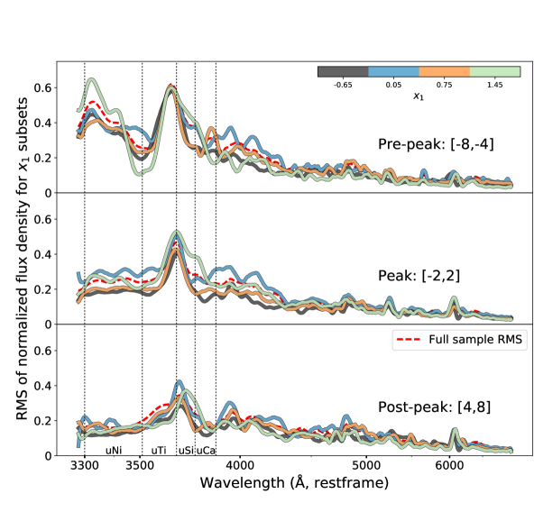
Figure 3: Intrinsic flux RMS (vs. wavelength) for SNe after division into four bins according to increasing lightcurve width (dark to light lines). Spectra were initially normalized to have median flux of unity over the $[3300,6900]$ Å wavelength region. Panels from top to bottom show the three sample phase regions (pre-peak, peak and post-peak). Vertical (dotted) lines mark boundaries of the four U-band regions. The red dashed red line shows the RMS for the full sample.

The mean dereddened spectrum, and the $1\sigma$ sample variation, for each phase bin after dereddening and normalizing to a common median $B_{\mathrm{SNf}}$-band flux, can be seen in Fig. 2. The large variation in the Ca H&K+Si ii feature is obvious at pre-peak phases. Also, the bluest region ($\lambda($uNi$)$) shows large early variation. At roughly one week after peak, the dispersion has significantly decreased at all wavelengths. This RMS vs wavelength is directly displayed as the dashed red line in Fig. 3 with normalization to a wider wavelength range. Here, we also show the dispersion of subsets of the sample, divided according to the SALT2.4 $x_{1}$ parameter and with the mean recalculated for each subset. All subsets show scatter similar to that of the full sample, with the possible exception of the post-peak $\lambda($uTi$)$ region. The variability in the post-peak phase bin can be described as a smooth component, only slowly declining with wavelength, with Si line variability superimposed. The $\lambda($uNi$)$ RMS here is $0.16$ mag, comparable to that of the $B_{\mathrm{SNf}}$-band ($0.14$ mag).

3.2 Spectroscopic variations with common SN Ia properties

Here we examine how the U-band varies with commonly used SN Ia properties by comparing composite spectra generated from subsets of the data. These are shown in Figs. 4 and  5. Subsets are constructed as follows: We retrieve all (restframe) spectra within a phase bin and normalize using the median flux of the $B_{\mathrm{SNf}}$ band. If a SN has two spectra from different nights within this range, the closest to the center of the bin is used. If the mean phase of two (sequential) spectra is closer to the center phase, their mean spectrum is used instead. At each phase we show four composite spectra constructed by dividing the full sample according to quartiles made from a secondary property, i.e. the $25\%$ SNe with lowest value form one subset, the next $25\%$ another and so forth. Quartile mean composites are shown, from low to high, with increasingly lighter colors (inverted for $x_{1}$). A spectral feature correlation with the secondary property, spanning the full sample and not driven by outliers, will lead to all subset composites being arranged in ”color” order. Through examination of these panels we observe the following:

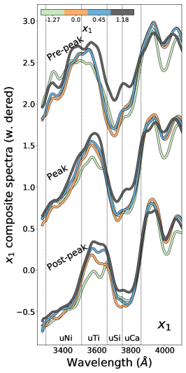
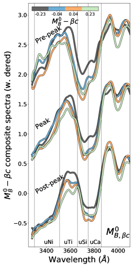
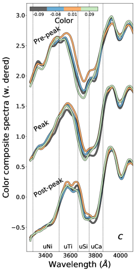
Figure 4: U-band spectroscopic variation spanning the range of common SN properties: $x_{1}$, dereddened $M_{B}$, $\mathrm{Color}$ (left to right). Composite spectra were calculated after dividing the sample into four quartiles based on each property, which was repeated at three representative phase ranges ($-6$, $0$, $6$) for each subset. Subset composites were drawn such that the line color becomes darker as the parameter value decreases. Dotted lines indicate U-band spectral-index sub division boundaries.

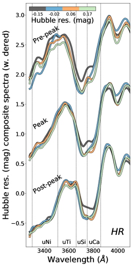
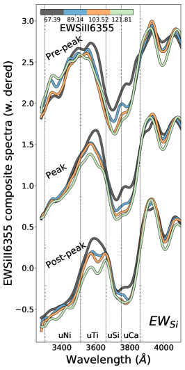
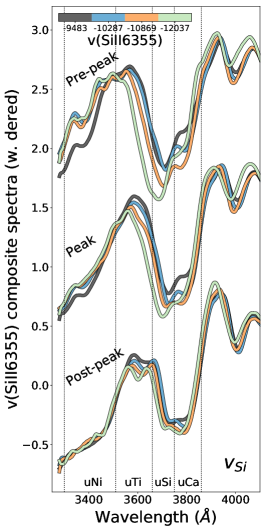
Figure 5: U-band spectroscopic variation spanning the range of common SN properties: Hubble residuals standardized by SALT2.4 lightcurve parameters, EW(Si ii $\lambda 6355$) and v(Si ii $\lambda 6355$) (left to right). Composite spectra were calculated after dividing the sample into four quartiles based on each property, which was repeated at three representative phase ranges ($-6$, $0$, $6$) for each subset. Subset composites were drawn such that the line color becomes darker as the parameter value decreases. Dotted lines indicate U-band spectral-index sub division boundaries.

• $x_{1}$ and $M^{0}_{B,\beta c}$ (lighcurve width/luminosity): The shallow Intermediate Mass Element (IME) features of slow-declining supernovae are seen in the Ca H&K $\lambda\leavevmode\nobreak\ 3945$ feature at all times (lightly shaded line). Besides this, the dominant feature is the strong correlation of the uTi-feature flux level with luminosity/lightcurve width. This dependence grows stronger after peak.

• Color: We find no signs of persistent feature variations with SALT2.4 color after dereddening, thus visually confirming that our dereddening procedure worked as intended.

• SALT2.4 standardization residuals: We identify the pre-peak uCa and uTi indices as potentially interesting for use in standardization.

• EW(Si ii $\lambda 6355$): The width of several features vary with EW(Si ii $\lambda 6355$), including Ca H&K+Si ii, EW(Si ii $\lambda 4138$), and uTi at late phases. This suggests that the Branch et al. (2006) subdivision into SNe Ia with broader/narrower spectral features is present, to some extent, in the U-band.

• v(Si ii $\lambda 6355$): As expected, SNe Ia with large Si velocities at peak also demonstrate blueshifting in the Si ii $\lambda 3858$ and Si ii $\lambda 4138$ features.

4 Results: Understanding the explosion

4.1 Origin of U-band index variations

We use synthetic YNAPP fits to determine which element changes are needed to remove the dissimilarities between the SN2011fe and SN20080514-002 spectra. YNAPP is a C implementation of the original ynow \ code (\verb syn++ ) with an added optimizer, to find the best ion temperature, velocity and optical depth combinations to fit input spectra under the obolev approximation for e^- scattering (Thomas et al., 2011). Fits presented here include Mg ii, Si ii, Si iii, S ii, Ca ii, Ti ii, Fe ii, Fe iii, Cr ii, Co ii, Co iii , Ni ii. We focus on the region bluewards of the Ca H&K+Si ii region and thus do not attempt to reconstruct Ca H&K+Si ii HVFs. No detached ions were included. The full fits including these ions capture the observed spectra well. Fits were also remade while iteratively deactivating one (or a combination) of the ions.

4.1.1 $\lambda($uNi$)$: $3300$ – $3510$ Å

SYNAPPS fits and their implication for the $\lambda($uNi$)$ spectroscopic region are shown in Fig. 6. We find that the $\lambda($uNi$)$ window can be tied to the presence of Ni and Co , the decay product of ⁵⁶Ni at these phases. Other elements, investigated using YNAPP  runs without Ni/Co, cannot replicate the observed spectra without distorting other parts of the spectrum. The effects of Ni and Co can be directly seen by manually decreasing the optical depths of these ions relative to the SN2011fe fit: a change of order $1$ dex creates a yn++ \ pectrum that matches SNF20080514-002 well in the $\lambda($uNi$)$ region (lower panels of Fig. 6). We show contributions of all included ions to the full fit in the Appendix (Figure 16). Tanaka et al. (2008), using abundance modifications to the W7 density profile to fit SN2002bo, also found this wavelength region to be sensitive to the amount of outer Ni (see their Fig. 2). Similar results can be seen in a number of studies using different techniques: Blondin et al. (2013) presented one-dimensional delayed-detonation models that show Co ii to dominate here; Hachinger et al. (2013) performed a spectral tomography analysis of SN2010jn where an early spectrum was dominated by Fe absorption at $3000$ Å and the Ni /Co around $3200$ Å, and a SYNAPPS study by Smitka et al. (2015) also shows strong Ni /Co absorption at $\sim 3300$ Å (although no Cr or Ti was included in these fits). Like Hachinger et al. (2013), we find that measurements of this spectral region are necessary for determining the spatial distribution of IGE elements, a key characteristic distinguishing theoretical explosion models. Cartier et al. (2017) found that V II provided improved fits to very early spectra of SN2015F, which would also impact the $\lambda($uNi$)$ region.

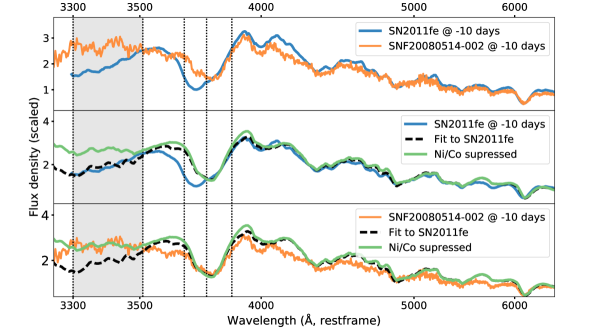
Figure 6: Probing the origin of variation in the $\lambda($uNi$)$ region through SYNAPPS model comparisons. The top panel compares SN2011fe and SNF20080514-002 at an early phase ($-10$ days). The second panel repeats the early SN2011fe spectrum (blue line) together with the best SYNAPPS fit (black dashed line). The green line shows the same fit, but with the optical depth ($\tau$) of all Ni and Co ii decreased by one dex, effectively suppressing these ions. The third panel compares the early SNF20080514-002 spectrum with the same SN2011fe SYNAPPS fits. The SN2011fe fit with suppressed Ni , Co ii optical depth matches the SNF20080514-002 $\lambda($uNi$)$ region well. Vertical dotted lines indicate the U-band spectral index boundaries, with $\lambda($uNi$)$ lightly shaded grey.

4.1.2 uTi : $3510$ – $3660$ Å

SYNAPPS fits and their implication for the $\lambda($uTi$)$ region are shown in Fig. 7. Among the YNAPP  ions included, only Ti ii produces significant absorption in the $3510$ to $3660$ Å region without distorting other parts of the spectrum. We display this association by manually decreasing the Ti ii optical depth. We do this for SNF20080514-002 since it shows the larger absorption, and again find that a change of order $-1$ dex produces a spectrum that matches the SN2011fe uTi region well. More complete radiative transfer models are needed to determine whether uTi variations are fully explained by Ti ii absorption, but we note that the Ti lines at $3685$, $3759$ and $3761$ Å would land in the uTi wavelength region for typical SN Ia velocities. The post-peak $\lambda($uTi$)$ region is, as can be seen in Figs. 4 and 5, strongly correlated with EW(Si ii $\lambda 6355$). As no strong Si lines are expected in this region this reflects a general connection between widths of spectroscopic features in SN Ia spectra. We show contributions of all included ions to the full fit in the Appendix (Fig. A17).

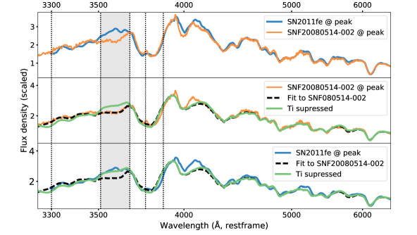
Figure 7: Probing the origin of uTi variation through SYNAPPS model comparisons. The top panel compares SN2011fe and SNF20080514-002 at peak light. The second panel shows SNF20080514-002 (orange line) together with the best SYNAPPS fit of this spectrum (black dashed line). The green line shows the same fit, but with the optical depth ($\tau$) of Ti ii decreased by one dex, effectively suppressing these ions. The third panel compares the SN2011fe spectrum with the same SNF20080514-002 SYNAPPS fits. The SNF200805014-002 fit with suppressed Ti ii optical depth matches the SN2011fe $\lambda($uTi$)$ region well. Vertical dotted lines indicate the U-band spectral index boundaries, with $\lambda($uTi$)$ shaded light grey.

4.2 Explosion models and progenitor scenarios

The single degenerate scenario – mass transfer from a red giant or main sequence star onto a Carbon-Oxygen White Dwarf – is no longer considered as likely to explain all (or most) SNe Ia. Challenges come from the lack of companion stars close to nearby SNe (e.g. SN2011fe Li et al., 2011; Schaefer & Pagnotta, 2012; Edwards et al., 2012), the statistical absence of early lightcurve variations due to ejecta interaction with the companion (Hayden et al., 2010), an insufficient number of such systems formed (Ruiter et al., 2011), and a large range of ejecta masses (Scalzo et al., 2014). A number of scenarios, possibly existing in parallel, are currently being investigated. These predict similar spectral energy distributions in the $4000$ to $7000$ Å region around lightcurve peak and have thus proven hard to rule out using such data (Röpke et al., 2012). Bluer wavelengths, on the other hand, show significant differences between current theoretical models. We have compared output spectra from delayed detonation (model N110, Seitenzahl et al., 2014; Sim et al., 2013), violent merger (model 11+09, Pakmor et al., 2012), sub-Chandra double detonation (model 3m, Kromer et al., 2010) and sub-Chandra WD detonation (Sim et al., 2010) models. We find that none of these describe the observed U-band variations.

Miles et al. (2016) found constant Si but varying Ca abundances to be a robust consequence of changing the progenitor model metallicity. However, they do not find this to cause strong changes in the observed spectra. We have nonetheless searched for uCa changes, not visible in uSi, for indications of a relationship to metallicity, but did not observe anything significant. The region identified by Miles et al. (2016) as strongly and consistently affected by metallicity was the Ti absorption at $\sim 4300$ Å at $\sim 30$ days after explosion. As this feature, as for the uTi index, is strongly correlated with peak luminosity and lightcurve width, searching for a second order variation due to metallicity is challenging.

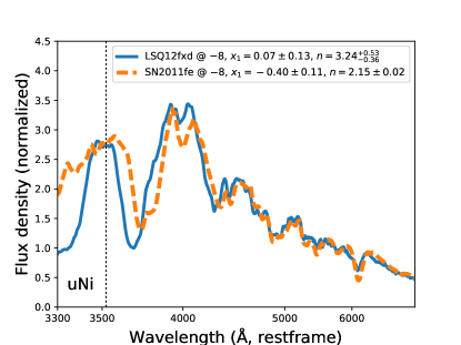
Figure 8: Spectra of SN2011fe and LSQ12fxd at phase $\sim-8$ days. LSQ12fxd has, compared with SN2011fe, both a steeper early rise-time (Firth et al., 2015) and less flux in the $\lambda($uNi$)$ region (i.e. stronger Co ii absorption at this phase).

A more direct way to probe Ni in the outermost layer is through observation of the very early lightcurve rise-time, parameterized as $f\propto t^{n}$. A mixed ejecta (shallow ⁵⁶Ni) will cause an immediate, gradual flux increase while deeper ⁵⁶Ni with cool outer layers experience a few days of dark time before a sharply rising lightcurve (Piro & Nakar, 2014; Piro & Morozova, 2016). In these models, the effects of outer ejecta mixing has largely disappeared $\sim$ one week after explosion. Firth et al. (2015) examine a sample of SNe with very early observations, finding varying rise-time power-law indices $n$ between $1.48$ and $3.7$, suggesting that either the outermost ⁵⁶Ni layer and/or the shock structure varies significantly between events. A sample of SNe with both early lightcurve data and U-band spectra would allow a direct comparison between pre-peak $\lambda($uNi$)$ absorption and the amount of shallow Ni predicted from the early lightcurve rise-time.

SN2011fe and LSQ12fxd in the Firth et al. (2015) study are included in the sample studied here and have observations at a common phase of $\sim 10$ days before peak (shown in Fig. 8). Compared with SN2011fe, LSQ12fxd has both a steeper rise-time immediately after explosion ($n=3.24$ vs. $n=2.15$) and more Co ii absorption (less $\lambda($uNi$)$ flux) in the line-forming region one week prior to lightcurve peak. A scenario explaining both observations would involve ⁵⁶Ni mixed into the outermost ejecta regions in SN2011fe while being located slightly deeper and being denser in LSQ12fxd. The comparison is non-trivial as these SNe also vary significantly in lightcurve width and line velocities, but we note that neither $x_{1}$ nor v(Si ii $\lambda 6355$) correlates strongly with early uNi and that Firth et al. (2015) find no correlation between $n$ and lightcurve width.

5 Results: Impact on standardization

Here we discuss the strong correlation between post-peak uTi and peak luminosity, and the potential impact of uCa, for SN Ia standardization (Sec. 5.1). The residual magnitude correlation with host environment after standardization is explored in Sec. 5.2. In Sec. 5.3 we explore whether the systematic effects from reddening corrections could significantly affect these results.

5.1 SN Ia luminosity standardization with uTi and uCa

Many spectroscopic features show strong correlations with SN Ia luminosity. These include $\mathcal{R}($Si$)$ and $\mathcal{R}($Ca$)$, introduced by Nugent et al. (1995), and the equivalent width (or “strength”) of the Si ii $\lambda 4138$ feature (Arsenijevic et al., 2008; Chotard et al., 2011; Nordin et al., 2011). As discussed in Sec. 3.2, uTi displays a similarly strong sensitivity to peak luminosity, especially at post-peak phases where contamination by the blue edge of the Ca H&K $\lambda\leavevmode\nobreak\ 3945$ feature is less likely. For some SNe a direct connection to $\mathcal{R}($Ca$)$, measured as the ratio between flux at the edges of the Ca H&K $\lambda\leavevmode\nobreak\ 3945$ feature, could exist. We now further explore the uTi-luminosity correlation.

In Fig. 9 (mid panel) we show the uTi change with phase per SN, and with measurements color-coded by lightcurve width (SALT2.4 $x_{1}$). From around lightcurve peak and later, we find a persistent and strong relation, where SNe with wider lightcurves have bluer uTi colors. To confirm that this correlation is not driven by the dereddening correction or changes in the $B_{\mathrm{SNf}}$ band, Fig. 9 contains two modified color curves: The first (left panel) shows the observed color $\mathrm{uTi}_{\mathrm{obs,B}}$, i.e. uTi recalculated according to Equation 1 but without dereddening spectra, and the second (right panel) shows the $B_{\mathrm{SNf}}-V_{\mathrm{SNf}}$ color evolution (calculated based on restframe and dereddened spectra). We confirm that the strong $x_{1}$ trend is present also without dereddening but not visible for $B_{\mathrm{SNf}}-V_{\mathrm{SNf}}$.

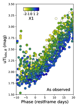
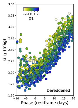
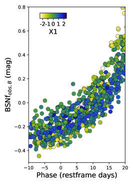
Figure 9: uTi vs. phase with markers colored by SALT2.4 $x_{1}$. Left panel shows the uTi color prior to F99 dereddening, mid panel after this correction. The right panel displays the $B_{\mathrm{SNf}}-V_{\mathrm{SNf}}$ color evolution for reference, calculated from dereddened restframe spectra. Pre-peak observations show a scatter induced by the edge of the Ca H&K $\lambda\leavevmode\nobreak\ 3945$ feature. uTi colors after peak show a strong stable correlation with lightcurve width.

We evaluate SN Ia standardization using combinations of post-peak uTi as a replacement for $x_{1}$, and pre-peak uCa as an additional standardization parameter (see Table 2). We assume a fixed $\Lambda CDM$ cosmology, continue to remove red SNe ($c>0.2$) and use SNe in the $0.03<z<0.1$ range to reduce scatter from peculiar velocities. We further fix the SALT2.4 $\beta$ parameter (the magnitude dependence of $c$) to the (blinded) value determined from the full SNfactory sample (derived without cuts based on color or first phase). The two base fits include either the magnitude dependence of $x_{1}$ (“$\alpha$”) or the magnitude dependence of post-peak uTi. Two permutations of these are made: one (“cut”) where the sample is limited to SNe with observations at all phases (early and late), and another where pre-peak uCa is added as a second standardization parameter. To allow comparisons of $\chi^{2}$ between runs we add a fixed dispersion of $0.090$ mag, the value required to produce ${\chi^{2}/\mathrm{dof}=1}$ for the initial $x_{1}$ run (first row in table). The uncertainty of each U-band index is composed of the sum of variance due to statistical uncertainties of the spectra and the propagated reddening variance, and is generally at the $\sim 0.03$ mag level (see Table 4). The measurement correlations between U-band indices and SALT2.4 fit parameters are negligible.

Table 2: Standardization fit results.

Fit parameters	SNe	$\chi^{2}$	$\chi^{2}/$dof	HR RMS (mag)	Host mass step (mag)	LsSFR step (mag)
$x_{1}$	$73$	$70.76$	$1.00$	$0.135\pm 0.011$	$0.098\pm 0.031$	$-0.151\pm 0.028$
uTi@p6	$57$	$44.18$	$0.80$	$0.116\pm 0.011$	$0.042\pm 0.031$	$-0.075\pm 0.031$
$x_{1}$ (cut)	$43$	$43.22$	$1.05$	$0.136\pm 0.015$	$0.094\pm 0.037$	$-0.156\pm 0.035$
uTi@p6 (cut)	$43$	$27.21$	$0.66$	$0.105\pm 0.012$	$0.034\pm 0.033$	$-0.068\pm 0.034$
$x_{1}$ + uCa@m6	$52$	$40.90$	$0.83$	$0.122\pm 0.012$	$0.081\pm 0.033$	$-0.138\pm 0.030$
uTi@p6 + uCa@m6	$43$	$18.22$	$0.46$	$0.086\pm 0.010$	$0.022\pm 0.030$	$-0.065\pm 0.030$

Our primary conclusion is that post-peak uTi standardizes SNe Ia very effectively, with an RMS of $0.116\pm 0.011$ mag. A traditional $x_{1}$ standardization yields a higher RMS of $0.135\pm 0.011$ mag for these SNe. This is remarkable in many aspects: it is a single color measurement made in a fairly wide phase range and using a fixed wavelength range that produces a lower $\chi^{2}$ fit. For the reduced sample of $57$ SNe with both measurements this is an improvement over $x_{1}$ with $\Delta\chi^{2}=$ $20.5$, which is significant at greater than $3\,\sigma$ (see also Table 3). We further investigate the potential effects of sample selection by redoing the fits based on a “cut” sample, where only SNe with both pre-peak ($-8$ to $-4$ days) and post-peak ($4$ to $8$) data are included. We see no significant differences between the full and cut samples. The reduced dispersion for uTi fits is thus not due to sample selection.

The Spearman rank correlation coefficient between SALT2.4 Hubble residuals and pre-peak uCa is $r_{s}=$ $0.43$, and the hypothesis of no correlation can be rejected at greater than $99\%$ confidence (Fig. 10, left panel). We therefore test adding pre-peak uCa measurements as a further standardization parameter. Combining post-peak uTi and pre-peak uCa produces a Hubble diagram RMS of $0.086\pm 0.010$ mag, while using only uCa and $x_{1}$ reduced the RMS to $0.122\pm 0.012$ mag. The driving trend of this improvement can also be seen in Fig. 10: SNe Ia with large uCa index are too bright after SALT2.4 standardization. Half of these are classified as Branch Shallow Silicon objects – this connection is further explored in Sec. 6.1.

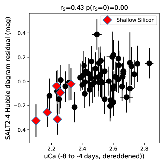
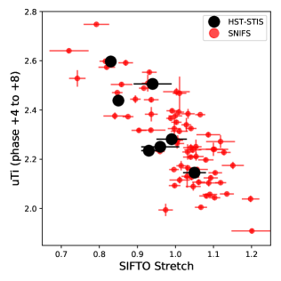
Figure 10: Left: Origin of pre-peak uCa correlation with SALT2.4 Hubble residuals. The Spearman correlation coefficient of $r_{s}=$ $0.43$ indicates a moderate correlation, with the hypothesis of no correlation at $>99\%$ confidence. Right: Comparing the post-peak uTi color integrated from HST-STIS spectra with SIFTO stretch. Spectra were dereddened according to a similar procedure as the SNfactory sample and use lightcurve data from Maguire et al. (2012). The SNIFS sample presented here is included for comparison, with SALT2.4 $x_{1}$ values converted to SIFTO stretch using the relation provided by Guy et al. (2010). The trend with uTi agrees betwen these two data sets.

We also note that the combined uTi + uCa fit produces a much reduced $\chi^{2}$ value, beyond what can be expected just through adding another fit parameter. When rerunning the standardization without a fixed intrinsic dispersion we obtain $\chi^{2}=38.6$ for $40$ degrees of freedom, thus there is no need to add any additional dispersion to reach $\chi^{2}/\mathrm{dof}=1$. As the internal SALT2.4 model error propagates an effective intrinsic dispersion of $0.055$ mag, other fit methods are required to investigate whether a fit without any added dispersion can be attained. For comparison, the uTi fit requires an intrinsic dispersion of $\sigma_{int}=$ $0.070\pm 0.009$ mag and the $x_{1}$ fit requires $\sigma_{int}=$ $0.090\pm 0.008$ mag.

Table 3: Each line shows Hubble residual fit quality for a given standardization method, measured relative to a reference fit based on post-peak uTi data without any host property corrections (first line). Each comparison is made using only the SNe in common (Nbr SNe) for a given measurement. The penultimate column shows the difference in $\chi^{2}$ assuming Hubble residuals are described using one or two Gaussian distributions (the latter when a host property step is included). The final column gives the likelihood according to the the sample-size corrected Akaike Information Criteria (AICc), again relative to the first line uTi model.

Standardizing property	Host step	Nbr SNe	$\chi^{2}-\chi^{2}_{uTi}$	P(AICc) Ratio
uTi@p6	None	$57$	$0$	$1.0$
	Global mass	$47$	$-1.9$	$0.19$
	LsSFR	$47$	$-4.8$	$0.84$
$x_{1}$	None	$57$	$20.5$	$3.6e-5$
	Global mass	$47$	$5.6$	$0.0045$
	LsSFR	$47$	$1.9$	$0.029$
uTi@p6 + uCa@m6	None	$43$	$-17.2$	$1521.5$
	Global mass	$35$	$-12.0$	$5.0$
	LsSFR	$35$	$-15.9$	$33.7$

As a further test we evaluate the fit quality using the sample-size corrected Akaike Information Criteria (AICc), which penalizes models with additional fit parameters. In Table 3 each line compares uTi standardization (without any host galaxy property correction) with one other combination of standardization property and host parameter. Each comparison includes all SNe available for that combination of data, and shows both the difference in $\chi^{2}$ and the AICc probability ratio. Models including both uTi and uCa are strongly preferred over only using uTi, with a P-value of $<0.001$, even though penalized for adding another fit parameter. Using only uTi is similarly favored compared with the $x_{1}$ fit.

The significance of these improvements can also be numerically investigated by re-fitting the standardization after randomly redistributing the uCa measurements among SNe. When coupled to uTi, two out of $10000$ random simulations yielded a similarly low RMS, equivalent to a $P$-value of $<10^{-5}$. When combined with $x_{1}$, zero out of $10000$ did so.

Finally, the HST-STIS sample presented by Maguire et al. (2012) also included a small sample of spectra covering the $\lambda($uTi$)$ region and overlapping with the post-peak phase studied here (phase $+4$ to $+8$ days). Lightcurve width information (“stretch” and $B-V$, determined by SIFTO) exists for seven of these SNe (PTF10wof, PTF10ndc, PTF10qyx, PTF10qjl, PTF10yux, PTF09dnp, PTF10nlg). With these data we can check an external dataset for a similar correlation. We deredden the spectra as was done previously with the SNf data and calculate the uTi color. Fig. 10 (right panel) shows a strong correlation for this small sample, compatible with the uTi trend discussed above. We find that this trend agrees well with the SNIFS measurement presented here, after converting the latter to SIFTO stretch values.

5.2 The SN progenitor environment

The R17 analysis of the local host galaxy environment found that SNe Ia in younger environments are $0.163\pm 0.029$ mag ($5.7\sigma$) fainter than SNe Ia in older environments, after SALT2.4 standardization (based on a larger sample than used here). The corresponding analysis of global host galaxy mass found SNe Ia in lower mass galaxies to be $0.119\pm 0.032$ mag fainter than those in more massive hosts. We recover these trends for the subset of SNe in this analysis with R17 measurements, finding a $-0.151\pm 0.028$ mag step for LsSFR and $0.098\pm 0.031$ mag for global host galaxy mass.

When this step analysis is performed based on the standardization residuals where uTi replaced $x_{1}$ the step sizes are reduced to $0.042\pm 0.031$ mag for mass and $-0.075\pm 0.031$ mag for LsSFR (given in the final two columns of Table 2). uCa has less impact for environmental steps, producing modest step size reductions to $0.022\pm 0.030$ mag and $-0.065\pm 0.030$ mag. $\Delta\chi^{2}$ and AICc probabilities for these models, again relative to applying uTi but no host data, can also be found in Table 3. We find that the full model including uTi, uCa and LsSFR provides the smallest $\chi^{2}/\mathrm{dof}$, but that the AICc find fits including uTi and uCa but no host corrections to be preferred considering the number of parameters. The fit quality of the $x_{1}$ models rapidly increases as host information is included. Adding host information to the U-band parameter models is not justified as $\chi^{2}$ is only modestly improved.

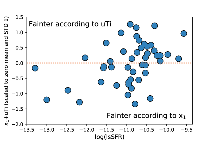
Figure 11: The difference in standardization based on $x_{1}$ and uTi is examined by comparing their sum (as they are anti-correlated) against local specific star formation (LsSFR). A smaller $x_{1}+$uTi (y-axis) value corresponds to a SN considered fainter according to $x_{1}$ relative to what uTi predicts.

In Fig. 11 we search for the SNe for which lightcurve width and uTi predict different magnitudes. As uTi and $x_{1}$ are anti-correlated, we can do this by normalizing both distributions to zero mean and unity RMS and then plotting the sum of the two transformed values for each SN. Current $x_{1}$ standardization produces SN magnitudes that are too bright in passive environments (low LsSFR), i.e. the $x_{1}$ parameter assumes these to be intrinsically fainter than they actually are and overcorrects their magnitudes. As is visualized in Fig. 11, uTi still predicts these SNe to be intrinsically faint, but not by as much as $x_{1}$, thus generating smaller magnitude corrections and avoiding overcorrection. Similarly, in actively star forming regions uTi does not predict SNe to be as intrinsically overluminous as predicted by $x_{1}$. The variation in predicted peak magnitude as a function of host galaxy environment suggests an underlying property that varies with age and affects the explosion duration (lightcurve width) without a corresponding change of the peak energy/temperature would cause a trend like the one observed. Further studies are needed to investigate whether, for example, progenitor size could act in this way.

The dependence on LsSFR can be visualized for this sample by comparing peak magnitude (for clarity, after color correction) versus SALT2.4 $x_{1}$ (left panel of Fig. 12). For fixed $x_{1}$, SNe in passive (“delayed”) environments are brighter. Performing such a comparison for uTi shows the dependence on LsSFR to be much reduced (right panel of Fig. 12).

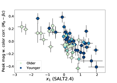
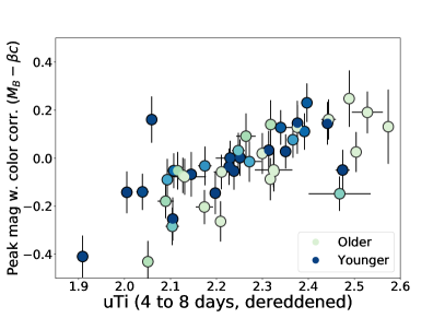
Figure 12: Comparing peak SN magnitude (including color correction) with SALT2.4 $x_{1}$ (left panel) and uTi (right panel). Lighter shaded points were found in R17 to originate in locally passive regions, and likely from old progenitors, while dark blue points were found in regions dominated by star formation. These are separated in $x_{1}$ (left), but not in uTi (right).

5.3 U-band indices and the choice of color curve

Here we first study the potential systematic error caused by dereddening using the F99 color curve, if in fact all SNe Ia actually followed the SALT2.4 color curve. The systematic (theoretical) change in the uNi, uTi, uSi and uCa color indices between F99 and SALT2.4, as a function of the color parameter is shown in Fig. 13. We use the same conversion between $E(B-V)$ and SALT2.4 $c$ as previously. More than $90\%$ of the sample has $|c|<0.15$, a range where the maximum possible variation for the uTi, uSi and uCa colors are limited to less than $0.1$ mag – small considering the U-band parameter value ranges found here. We therefore conclude that the standardization effects discussed above were not driven by systematic effects from the dereddening process.

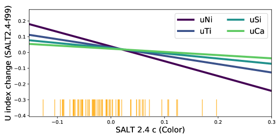
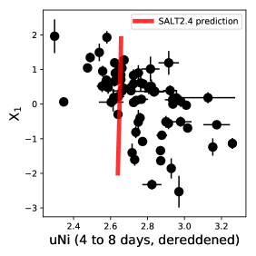
Figure 13: Left: Directly comparing the difference in U-band color indices, u(Ni—Ti—Si—Ca)^SALT-u(Ni—Ti—Si—Ca)^F99. While systematic differences grow large for highly reddened objects, these are limited for the current sample. Orange, short, vertical lines show the SALT2.4 $c$ values of SNe in this sample. Right: SALT $x_{1}$ vs uNi at phase $4$ to $8$ days. The red line shows the corresponding SALT model predictions.

An empirical SN Ia standardization model, like SALT2.4, relies on the combination of a color curve and a spectral model to predict how the intrinsic spectrum varies (for SALT the latter is parameterized by $x_{1}$). Comparing the SALT2.4 spectral model with observations in the $\lambda($uNi$)$ region, where empirical and dust color curves start to strongly deviate, we note a clear functional difference – the uNi color decreases with wider lightcurve width in a way that is not captured by the the SALT2.4 model (Fig. 13, right panel). Such a mismatch between the SALT2.4 template and the observed SED could, if correlated with broad-band colors, modify the derived effective color curve and potentially bias cosmological parameter constraints if the SN Ia sample distributions vary with redshift/look-back time.

6 Discussion

6.1 Literature subclasses

Table 4: Mean and its uncertainty of Hubble diagram residual for Branch Shallow Silicon and SN1991T-like SNe (the latter a subset of the former), for three different standardization methods, as discussed in Sec.5. Results shown are from the “cut” sample, for which the three standardization methods can be compared. Note that the uncertainties are highly correlated.

		$x_{1}$		uTi		uTi + uCa
Sample	Nbr	HR mean (mag)	$\chi^{2}$	HR mean (mag)	$\chi^{2}$	HR mean (mag)	$\chi^{2}$
SS	5	$-0.194\pm 0.052$	$14.4$	$-0.100\pm 0.058$	$8.0$	$-0.032\pm 0.051$	$4.4$
91T	2	$-0.279\pm 0.024$	$8.6$	$-0.190\pm 0.023$	$4.3$	$-0.095\pm 0.011$	$1.1$

A potential link with Shallow Silicon SNe (Branch et al., 2006) was highlighted in connection with uCa and SN standardization (Fig. 10). In particular, SN1991T-like objects, a core group among SS SNe, have flat early U-band spectra as one of their defining features (Filippenko et al., 1992; Scalzo et al., 2012). There are eight SS SNe in this sample, out of which two are SN1991T-like. Sub-classification of the SNfactory sample will be further discussed in Chotard et al. (in prep). Here we note that the mean Hubble diagram residual bias for SS and 91T-like objects gets progressively smaller when standardizing using U-band indices, as shown in Table 4. The two 91T-like SNe have very similar uNi index, EW(Si ii $\lambda 6355$) and Hubble residuals, while they are separated from both other SS SNe and other SN Ia subtypes (see Fig. 14, left panel). We find no evidence of a continuous distribution connecting these to the main SN population, further suggesting that these SNe are more closely related to Super Chandrasekhar-mass SNe Ia (see discussion in Scalzo et al., 2012, 2014).

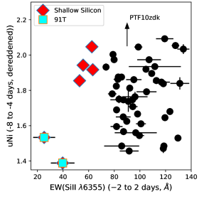
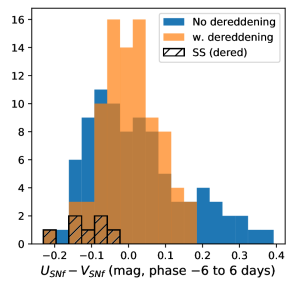
Figure 14: Left: uNi index measurements of SN1991T-like and Shallow Silicon-like SNe Ia compared with EW(Si ii $\lambda 6355$). The SN1991T-like SNe are disconnected from the remaining sample. Right: Distribution of $U_{\mathrm{SNf}}-V_{\mathrm{SNf}}$ for spectra within $6$ days of lightcurve peak. The figure shows data with (orange) and without (blue) reddening correction, where the linear evolution with phase was removed for each (returning distributions with zero mean). The Shallow Silicon (SS) subset of the dereddened $U_{\mathrm{SNf}}-V_{\mathrm{SNf}}$ distribution is shown by the cross-hatched histogram.

Milne et al. (2013, 2015) have suggested that SNe Ia can be divided into two subsets based on the SWIFT u$-$v color at $\pm 6$ days from peak. In Fig. 14 we show the $U_{\mathrm{SNf}}-V_{\mathrm{SNf}}$ color as determined from a similar wide phase range. We do not find strong signs of distinct populations in the $U_{\mathrm{SNf}}-V_{\mathrm{SNf}}$ color, especially not after reddening corrections are applied. The SWIFT UVOT u band is bluer compared with $U_{\mathrm{SNf}}$ while $V_{\mathrm{SNf}}$ extends slightly redder than the UVOT v band, thus filter sensitivity differences possibly cause different intrinsic SN Ia features to be probed. Cinabro et al. (2017) did not find significant signs of subsets based on modeling ground-based photometry of more distant SDSS and SNLS SNe. Milne et al. (2013) also highlighted high-velocity SNe and/or Branch Shallow Silicon SNe as having blue u$-$v colors, trends compatible with our data and highlighted in Fig. 14. Finally, we note that Milne et al. (2013) showed both SN2011fe and SNF20080514-002 to have similar blue UVOT u$-$v colors, while our analysis began with the spectroscopic differences found between these two SNe (Fig. 1). This further points to the difficulty in constraining spectroscopic variations using broadband photometry, and vice versa.

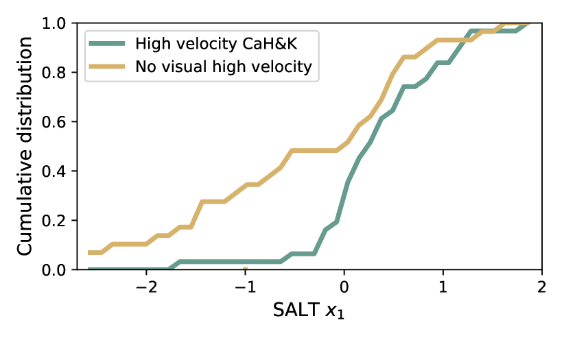
Figure 15: Cumulative $x_{1}$ distributions for SNe with and without visually identified High Velocity Features (based on spectra with phase $<-2$ day).

The existence of High Velocity Features has been another approach to subclassification involving U-band data. A blinded visual search for Ca HVFs was made with the purpose of dividing the sample into SNe with and without HVFs at phase $\sim-2$ days. All SNfactory spectra were randomly reordered and the Ca H&K $\lambda\leavevmode\nobreak\ 3945$ and Ca IR $\lambda 8579$ region displayed, together with the expected photospheric line position based on the Si ii $\lambda 6355$ velocity at that phase. A scanner (J.N.) classified each spectrum as either having clear HVF, having good data but no HVF or being too noisy for an accurate classification. For the small SN subset with multiple high S/N spectra prior to $-2$ days, we found the visual classification to agree, showing that we consistently classified these. We show the SALT2.4 $x_{1}$ cumulative distributions of SNe with and without the HVF classification in Fig. 15 (listed in Table. 4). As have previous studies (Childress et al., 2014; Silverman et al., 2015), we find narrower lightcurve SNe ($x_{1}\lesssim-0.5$) to only very rarely show HVFs at a phase whereas a majority of the $x_{1}>-0.5$ SNe show HVFs. A KS-test rejects a common parent population at greater than $99\%$ confidence. If the presence of HVFs were solely caused by, for example, the effective radius at a certain phase, to which $x_{1}$ could be correlated through the ejecta mass, a continously increasing probability of detecting HVFs would be expected. The data presented here is more suggestive of a rapid probability change with $x_{1}$, such as would be caused if $x_{1}\lesssim-0.5$ originate from a distinct explosion channel. In terms of the U-band spectral indices, this difference can be seen as a consistently small RMS for uSi and uCa at early phases among the low $x_{1}$-subset in Fig. 3.

6.2 Outlook

The wavelength limits of the U-band features used here were set based on a comparison of only two SNe, examined at two phases. These wavelength regions were then analyzed at three phase intervals chosen to roughly capture typical SN Ia spectral variations on weekly scales, but chosen prior to any knowledge regarding when certain features come to dominate. An improved future analysis will include phase-dependent wavelength regions, where observations at different phases are combined with appropriate weights. Integration of flux within fixed wavelength limits carry less stringent signal-to-noise requirements compared with measurements of individual spectroscopic features. Thus, low-resolution spectroscopy (or possibly narrow-band filters) could measure the U-band indices directly at high redshifts.

A sample of nearby SNe Ia with cadenced U-band spectroscopy starting at early phases ($<-10$ days) would allow novel studies of the explosion process through the temporal development of the $\lambda($uNi$)$ region. Simultaneously, Ca H&K $\lambda\leavevmode\nobreak\ 3945$ features map IME variations and uTi provides accurate temperature estimates after peak light. Such early data is also needed to finally determine whether the lack of HVFs among narrower lightcurve SNe is a consequence of a less energetic explosion, or if this signals a physically different explosion mechanism and/or circumstellar material.

The limit at which HVFs disappear ($x_{1}\sim-0.5$) agrees with where Scalzo et al. (2014), using SNfactory SNe with coverage extending to late phases, find that the derived ejecta mass ($M_{ej}$) points to sub-Chandrasekhar mass explosions. The seven SNe in the sample analyzed here with derived $M_{ej}$ and $M_{Ni}$ masses from Scalzo et al. (2014) are insufficient for further tests of $M_{ej}$ and $M_{Ni}$ correlations, again motivating larger samples which combine several types of observations. These could include also ejecta/Ni /IGE constraints derived through nebular Co ii lines (Childress et al., 2015), second maximum position (Dhawan et al., 2015) and early lightcurve rise-time (Firth et al., 2015), as well as measurements of ejecta asymmetry from nebular lines (Maeda et al., 2011).

We see signs that the currently most widely used SN model, SALT2.4, can be improved. Updates to the SN template in this region could propagate into a change in the effective color law. Creating an unbiased template for the intrinsic U-band spectrum is a requirement for current and future ground-based SN Ia analyzes like DES and LSST, where the rest-frame U-band is redshifted to the wavelengths most efficiently observed from the ground.

7 Summary and conclusions

Comparing spectra of two supernovae at early and peak phases led to the subdivision of the U-band into four regions whose flux ratio relative to B-band were used to construct the uNi, uTi, uSi and uCa indices. We use a sample of $92$ SNe Ia to analyze these indices at three representative phase ranges: $-8$ to $-4$ days (pre-peak), $-2$ to $2$ days (peak) and $4$ to $8$ days (post-peak). Based on these measurements we find:

• SYNAPPS comparisons show that Ni/Co absorption can explain differences in the bluest feature (“uNi”). uNi at pre-peak phases can be used as a probe of Ni abundance, to complement constraints from the early lightcurve rise-time, bolometric lightcurves and nebular emission.

• In similar tests, SYNAPPS fits also show that Ti absorption differences dominate the $\lambda($uTi$)$ wavelength range. The uTi index is an extremely sensitive luminosity indicator. When used instead of the SALT2.4 $x_{1}$ parameter the RMS scatter around the Hubble diagram falls to $0.116\pm 0.011$ mag. Here we use measurements made in the post-peak phase region, but note that the uTi index at all phases after peak is strongly correlated with lightcurve width.

• Adding pre-peak uCa as a third standardization parameter further reduces the RMS around the Hubble diagram. A fit with uTi and uCa yields a $0.086\pm 0.010$ mag scatter with $\chi^{2}/\mathrm{dof}\sim 1$ without the need to introduce intrinsic dispersion.

• Including U-band indices in SN Ia standardization reduces the dependence on host-galaxy environment. The difference between lightcurve width and uTi can be used to study SN Ia progenitor scenarios.

• Shallow Silicon and 91T-like SNe have biased SALT2.4 Hubble residuals, which are substantially reduced when U-band parameters are included in the fit. The two 91T-like SNe in this sample have similar U-band properties and magnitudes, which are offset from the remaining sample.

• We confirm previous results that narrower-lightcurve SNe Ia very rarely show HVFs. We find a sharp transition in their incidence at $x_{1}=-0.5$.

Appendix A Element contributions to SYNAPPS fits.

We discuss in Sec. 4.1 how the observed spectral differences between SN2011fe and SNF20080514-002 can be explained by changing the early Ni/Co abundance and Ti abundance at peak. Here we show the complete set of ion contributions to the best fit SYNAPPS spectrum of SN2011fe $10$ days prior to peak (Fig. 16) and for SN200805014-002 close to peak (Fig. 17). These fits match the observed data well.

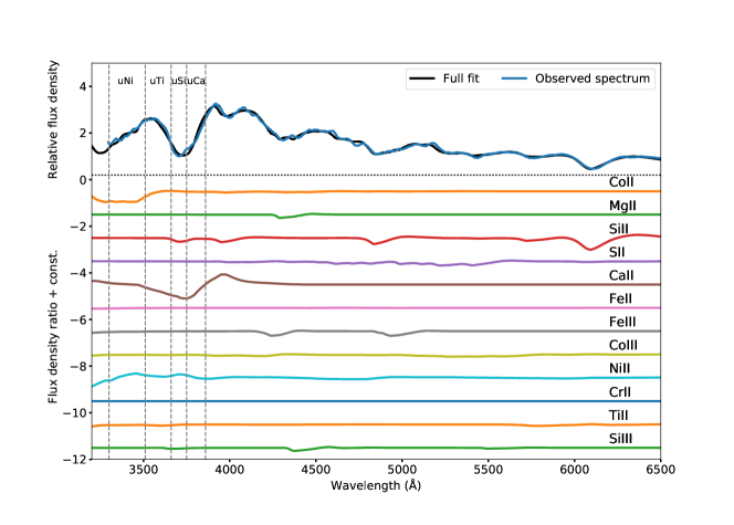
Figure 16: SYNAPPS fit to SN2011fe $10$ days prior to peak. The top panel compares the observed spectrum to the full SYNAPPS fit. The lower panels show the contribution of each ion to the final spectra. These are plotted as the ratio between the spectrum with and without each ion activated. Dashed, vertical, grey lines indicate the U-band index region boundaries, with designations given at the top.

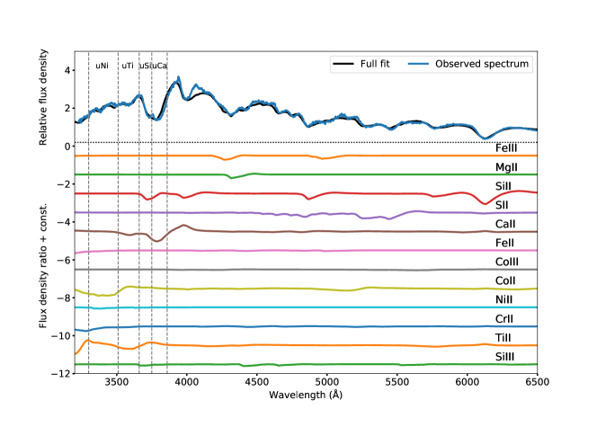
Figure 17: SYNAPPS fit to SNF20080514-002 at peak light. The top panel compares the observed spectrum to the full SYNAPPS fit. The lower panels show the contribution of each ion to the final spectra. These are plotted as the ratio between the spectrum with and without each ion activated. Dashed, vertical, grey lines indicate the U-band index region boundaries, with designations given at the top.