The Simplest Form of the Lorentz Transformations

Abstract

We report the simplest possible form to compute rotations around arbitrary axis and boosts in arbitrary directions for 4-vectors (space-time points, energy-momentum) and bi-vectors (electric and magnetic field vectors) by symplectic similarity transformations. The Lorentz transformations are based exclusively on real $4\times 4$-matrices and require neither complex numbers nor special implementations of abstract entities like quaternions or Clifford numbers. No raising or lowering of indices is necessary. It is explained how the Lorentz transformations can be derived from the most simple second order Hamiltonian of general significance. Since this approach exclusively uses the real Clifford algebra $Cl(3,1)$, all calculations are based on real $4\times 4$ matrix algebra.

I Introduction

A great many derivations of the Lorentz transformation have already been given, and the subject, because of its pedagogical importance, still receives continues attention […]. Most of the analyses, following the original one by Einstein, rely on the invariance of the speed of light $c$ as a central hypothesis. That such an hypothesis, firmly based on experimental grounds, has had a crucial historical role cannot be denied. The chronological building of order of a physical theory, however, rarely coincides with its logical structure.
– J.M. Levy-Leblond LevyLeblond

P.A.M. Dirac, the discoverer of relativistic quantum theory, wrote that the “real importance of Einstein’s work was that he introduced Lorentz transformations as something fundamental in physics” Dirac80 . But, as we shall argue, it is Dirac’s theory and not Einstein’s, which uncovers that the Lorentz transformations are indeed as fundamental as Hamiltonian functions are fundamental, first of all in a mathematical, but consequently also in a physical sense.

The Lorentz transformations (rotations and boosts) can be expressed using different (though related) formulations. The respective form mainly depends on the type of vectorial system used to represent space and time coordinates . The most commonly promoted formulation of the Lorentz covariance are the vector and it’s generalization, the tensor formalism. As we shall demonstrate, these are neither algorithmically nor conceptually the simplest variant.

We shall demonstrate here that the simplest possible form of the Lorentz transformations (LTs) is a direct consequence of the use of Hamiltonian methods. It is the irreducible remainder after a visit in Ockham’s barber shop. Our approach follows the work of Kim and Noz Kim1981 and is closely related to (and inspired by) Dirac’s equation, Hestenes’ and Sobczyk’ space-time algebra (STA) STA ; GA and other Clifford algebraic approaches like the ones of Baylis Baylis or Salingaros Salingaros . However, our presentation differs from most others insofar as we derive a representation of the Lorentz transformations (LTs) directly from Hamiltonian methods by the use of $4\times 4$ Dirac matrices over the reals. This matrix form is physically significant as the LTs are shown to be isomorphic to general linear canonical transformations of a acting on two coupled canonical pairs $(q_{1},p_{1},q_{2},p_{2})$. This kind of transformation is also called symplectic similarity transformation Kim1981 .

In this representation physical observables like momentum and energy are not regarded as self-sufficient “fundamental” quantities. Instead they are related to (linear combinations of) second moments of phase-space distributions (see Ref. GLT ). In two previous publications we explained that and how this reinterpretation of the LTs leads to a reinterpretation of quantum electrodynamics as a science of statistical moments in spinorial phase space qed_paper ; osc_paper . The main advantage of this approach is that all central quantities that determine the motion of a charged particle in an electromagnetic field, including their precise relations, can be derived from a single conservation law, namely in the form of the classical Hamiltonian function of two coupled harmonic oscillators. The resulting form of the LTs is extraordinarily simple and straightforward.

I apologize, but theoretical physics is defined as a sequence of courses, each of which discusses the harmonic oscillator.
– Sidney Coleman ColemanQFT

In order to motivate our approach we describe the conventional vector formalism (CVF) and contrast it with the suggested formalism of symplectic similarity transformations in some detail.

II Space described by Vectors

A position or direction in space is most commonly represented by a vector. As well-known, in CVF a “vector” is represented by a $3\times 1$-matrix

$${\bf x}=\left(\begin{array}[]{c}x\\ y\\ z\end{array}\right)\,,$$ (1)

or ${\bf x}=(x,y,z)^{T}$ with the superscipt “T” for matrix transposition.

If we construct unit vectors in each direction, then we may write:

$${\bf x}=x\,{\bf e}_{x}+y\,{\bf e}_{y}+z\,{\bf e}_{z}$$ (2)

where

$$\begin{array}[]{rclrclrcl}{\bf e}_{x}&=&\left(\begin{array}[]{c}1\\ 0\\ 0\end{array}\right)\,,&{\bf e}_{y}&=&\left(\begin{array}[]{c}0\\ 1\\ 0\end{array}\right)\,,&{\bf e}_{z}&=&\left(\begin{array}[]{c}0\\ 0\\ 1\end{array}\right)\\ \end{array}$$ (3)

The scalar product (dot product) of two vectors can be implemented as a product of a transposed $3\times 1$-matrix times a $3\times 1$-matrix

$${\bf x}_{1}\cdot{\bf x}_{2}={\bf x}_{1}^{T}\,{\bf x}_{2}=x_{1}\,x_{2}+y_{1}\,y_{2}+z_{1}\,z_{2}\,.$$ (4)

Unfortunately, this form to represent a vector has the undesired feature that the scalar multiplication changes the algebraic dimension and yields - as the name suggests - a scalar. Strange enough, there is a second type of vector multiplication, the so-called “vector” or “cross” product, which requires an extra symbol, namely the cross, and has its own definition:

$$\begin{array}[]{rcl}{\bf x}_{1}\times{\bf x}_{2}&=&(y_{1}\,z_{2}-y_{2}\,z_{1})\,{\bf e}_{x}\\ &+&(z_{1}\,x_{2}-z_{2}\,x_{1})\,{\bf e}_{y}\\ &+&(x_{1}\,y_{2}-x_{2}\,y_{1})\,{\bf e}_{z}\\ \end{array}$$ (5)

At first sight the cross product is an speciality of $3$-dimensional space and has no generalization to arbitrary dimensions and no obvious place within a generalized vector- and matrix-algebra. However, the cross product is physically and geometrically indispensable. It represents real and measurable properties of $3$-dimensional physical space, namely the handedness of magnetic and gyroscopic forces. The need to define two different products indicates, that an unstructured “list” of coordinates does not adequately represent the structural properties of $3$-dimensional “physical” space.

II.1 Rotations

Let us consider the rotation of a vector ${\bf r}$ by an angle $\alpha$ about an arbitrary direction indicated by the unit vector ${\bf w}$. The derivation of an appropriate formula requires the computation of the vector-components parallel and perpendicular to ${\bf w}$ and it is helpful to use a drawing that clarifies the situation (see Fig. 1). Besides the $\sin()$- and $\cos()$-function mainly vector addition and the computation of scalar and cross-products are needed in order to decompose the vector into the component parallel and perpendicular to ${\bf w}$, respectively.

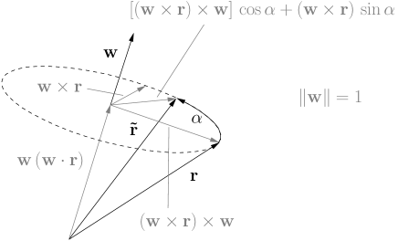
Figure 1: Rotation of an arbitrary vector ${\bf r}$ around arbitrary unit vector ${\bf w}$ with angle $\alpha$.

$$\begin{array}[]{rcl}{\bf r}&=&{\bf r}_{\parallel}+{\bf r}_{\perp}\\ {\bf r}_{\parallel}&=&({\bf w}\cdot{\bf r})\,{\bf w}\\ {\bf r}_{\perp}&=&({\bf w}\times{\bf r})\times{\bf w}\\ &=&{\bf r}-{\bf r}_{\parallel}={\bf r}-({\bf w}\cdot{\bf r})\,{\bf w}\\ {\bf\tilde{r}}&=&{\bf r}_{\parallel}+{\bf r}_{\perp}\,\cos{\alpha}+({\bf w}\times{\bf r})\sin{\alpha}\,.\end{array}$$ (6)

From this we can derive the most simple formula of CVF, the formula of Rodriguez:

$${\bf\tilde{r}}={\bf r}\,\cos{\alpha}+({\bf w}\times{\bf r})\sin{\alpha}+{\bf w}\,({\bf w}\cdot{\bf r})\,(1-\cos{\alpha})\,.$$ (7)

For the description of a supposedly fundamental operation like rotation in space, this formula is surprizingly complicate.

An alternative approach is the use of matrices to describe rotations. Since positions are represented in CVF by $3\times 1$ matrices, the rotation matrices ${\bf Q}_{x}$, ${\bf Q}_{y}$ and ${\bf Q}_{z}$ are orthogonal matrices of dimension $3\times 3$

$${\bf\tilde{x}}={\bf Q}_{k}(\alpha)\,{\bf x}\,.$$ (8)

where $k$ indicates a rotation axis. These rotation matrices are

$$\begin{array}[]{rcl}{\bf Q}_{x}&=&\left(\begin{array}[]{ccc}1&0&0\\ 0&\cos{\alpha_{1}}&-\sin{\alpha_{1}}\\ 0&\sin{\alpha_{1}}&\cos{\alpha_{1}}\\ \end{array}\right)\\ {\bf Q}_{y}&=&\left(\begin{array}[]{ccc}\cos{\alpha_{2}}&0&\sin{\alpha_{2}}\\ 0&1&0\\ -\sin{\alpha_{2}}&0&\cos{\alpha_{2}}\\ \end{array}\right)\\ {\bf Q}_{z}&=&\left(\begin{array}[]{ccc}\cos{\alpha_{3}}&-\sin{\alpha_{3}}&0\\ \sin{\alpha_{3}}&\cos{\alpha_{3}}&0\\ 0&0&1\\ \end{array}\right)\\ \end{array}$$ (9)

${\bf Q}_{x}$, ${\bf Q}_{y}$ and ${\bf Q}_{z}$ represent rotations around the coordinate axis ${\bf e}_{x}$, ${\bf e}_{y}$ and ${\bf e}_{z}$. These matrices can be obtained from the matrix exponential of “infinitesimal” rotations ${\bf R}_{k}$, which are simply the derivatives of the ${\bf Q}_{k}$:

$${\bf R}_{k}=\left.{d\over d\alpha_{k}}{\bf Q}_{k}(\alpha_{k})\right|_{\alpha_{k}=0}\,.$$ (10)

such that

$${\bf R}_{x}=\left(\begin{array}[]{ccc}0&0&0\\ 0&0&-1\\ 0&1&0\\ \end{array}\right)\,.$$ (11)

An infinitesimal rotation is then given by:

$${\bf\tilde{x}}=({\bf 1}+{\bf R}_{k}\,d\alpha_{k})\,{\bf x}\,.$$ (12)

The description of a general rotation of the vector ${\bf x}$ around an arbitrary axis $\vec{\omega}$ (with $|\vec{\omega}|=1$) can be done by a single matrix multiplication with a matrix ${\bf Q}$ which can be computed as the matrix exponential of the corresponding infinitesimal transformation:

$${\bf Q}=\exp{((\omega_{x}\,{\bf R}_{x}+\omega_{y}\,{\bf R}_{y}+\omega_{z}\,{\bf R}_{z})\,\alpha)}$$ (13)

It is explicitely given by

$${\bf\tilde{x}}=\left(\begin{array}[]{c}\tilde{x}\\ \tilde{y}\\ \tilde{z}\end{array}\right)=\left(\begin{array}[]{ccc}Q_{xx}&Q_{xy}&Q_{xz}\\ Q_{yx}&Q_{yy}&Q_{yz}\\ Q_{zx}&Q_{zy}&Q_{zz}\\ \end{array}\right)\,\left(\begin{array}[]{c}x\\ y\\ z\end{array}\right)$$ (14)

where

$$\begin{array}[]{rcl}Q_{xx}&=&c+(1-c)\,\omega_{x}^{2}\\ Q_{xy}&=&(1-c)\,\omega_{x}\,\omega_{y}-s\,\omega_{z}\\ Q_{xz}&=&(1-c)\,\omega_{x}\,\omega_{z}+s\,\omega_{y}\\ Q_{yx}&=&(1-c)\,\omega_{x}\,\omega_{y}+s\,\omega_{z}\\ Q_{yy}&=&c+(1-c)\,\omega_{y}^{2}\\ Q_{yz}&=&(1-c)\,\omega_{y}\,\omega_{z}-s\,\omega_{x}\\ Q_{zx}&=&(1-c)\,\omega_{x}\,\omega_{z}-s\,\omega_{y}\\ Q_{zy}&=&(1-c)\,\omega_{y}\,\omega_{z}+s\,\omega_{x}\\ Q_{zz}&=&c+(1-c)\,\omega_{z}^{2}\\ \end{array}$$ (15)

and $c=\cos{(\alpha)}$ and $s=\sin{(\alpha)}$. This way to describe rotations can, in principle, be extended to arbitrary dimensions, which means that it has no intrinsic connection to the dimensionality of space.

Surprisingly enough, the conventional rotation matrices ${\bf Q}_{k}$ are not directly used to describe the motion of rigid bodies in $3$-dimensional space. Instead, most textbooks recommend the use of Euler angles. The Euler angles are a powerful tool, but again are not simple or intuitive: Greiner for instance explains these angles with three figures Greiner . Even though the human mind is trained to grasp 3-dimensional situations, when it comes to real calculations, 3-dimensional space is remarkably tedious. This becomes even worse when Lorentz boosts and electromagnetic fields are considered as we shall see in Sec. II.2.

In the Hamiltonian Clifford algebra (HCA) suggested here, unit “vectors” are represented by real $4\times 4$-matrices $\gamma_{k}$ and the rotation of an arbitrary vector ${\bf x}=x\,\gamma_{1}+y\,\gamma_{2}+z\,\gamma_{3}$ around an arbitrary direction is generated by this same “direction”

$${\bf w}=\omega_{x}\,\gamma_{7}+\omega_{y}\,\gamma_{8}+\omega_{z}\,\gamma_{9}$$ (16)

applied to ${\bf x}$ in the form of a similarity transformation

$${\bf\tilde{x}}={\bf R}\,{\bf x}\,{\bf R}^{-1}$$ (17)

One should not be confused by the wording of “vector” and “matrix”. In the CVF, a “vector” is formally a column “matrix”. In the approach suggested here, a “vector” has the algebraic form of a matrix, not of a column matrix, but of a real $4\times 4$ matrix. This matrix may contain more information than that of a single column-“vector” and, as we shall show, it can be used to represent the structure of space-time and (quantum-) electrodynamics. Mathematically $4\times 4$ matrices can be used to represent specific Clifford algebras. But in case of matrices of dimension $2^{N}\times 2^{N}$, the reverse is true as well: Such matrices can always be represented in terms of Clifford algebras. This means that any real $2^{N}\times 2^{N}$-matrix can be expressed as a weighted sum of rather simple elementary matrices. We shall explain this in more detail in Sec. III.

Using a Clifford algebraic matrix decomposition, the transformation matrix ${\bf R}$ is again a matrix exponential of the generator ${\bf w}$

$${\bf R}=\exp{(-{\bf w}\,\alpha/2)}\,.$$ (18)

The “vector” ${\bf w}$, which represents the direction of rotation, has the same form as the “vector” ${\bf x}$, namely that of a $4\times 4$ Hamiltonian matrix. The unit matrices $\gamma_{7}$, $\gamma_{8}$ and $\gamma_{9}$ are simply products of two real Dirac matrices and are therefore called “bi-vectors”. They are defined by

$$\begin{array}[]{rcl}\gamma_{7}&=&\gamma_{2}\,\gamma_{3}\\ \gamma_{8}&=&\gamma_{3}\,\gamma_{1}\\ \gamma_{9}&=&\gamma_{1}\,\gamma_{2}\,.\end{array}$$ (19)

the form and meaning of which will be explained later.

All generators of rotations (like ${\bf w}$) square to $-{\bf 1}$ (i.e. are representations of the unit imaginary $i$), such that Eq. 18 yields Eulers formula:

$${\bf R}=\cos{(\alpha/2)}\,{\bf 1}-\sin{(\alpha/2)}\,{\bf w}\,.$$ (20)

The inverse transformation is given by the negative argument ${\bf R}^{-1}(\alpha)={\bf R}(-\alpha)$:

$${\bf R}^{-1}=\cos{(\alpha/2)}\,{\bf 1}+\sin{(\alpha/2)}\,{\bf w}\,.$$ (21)

The explicit form of the matrix is, in the chosen representation, given by:

$$\begin{array}[]{rcl}{\bf R}(\alpha)&=&{\bf 1}\,\cos{(\alpha/2)}-{\bf w}\,\sin{(\alpha/2)}\\ &=&\left(\begin{array}[]{cccc}c&-\omega_{y}\,s&\omega_{z}\,s&-\omega_{x}\,s\\ \omega_{y}\,s&c&\omega_{x}\,s&\omega_{z}\,s\\ -\omega_{z}\,s&-\omega_{x}\,s&c&\omega_{y}\,s\\ \omega_{x}\,s&-\omega_{z}\,s&-\omega_{y}\,s&c\\ \end{array}\right)\end{array}$$ (22)

where $c=\cos{(\alpha/2)}$, $s=\sin{(\alpha/2)}$.

Rotations, when expressed by a similarity transformation (Eq. 17), require two instead of one matrix multiplication(s) as in Eq. 14. One might therefore doubts that this symplectic method is really “simpler”. But firstly Eq. 17 can simultaneously be used to rotate not only the vector ${\bf x}$, but two bi-vectors as well, i.e. three different “vectors”. Secondly, the exact same form of matrix multiplication can be used to compute Lorentz boosts as well, as we shall demonstrate next.

Thirdly the use of the Hamiltonian Clifford algebras allows to relate geometrical to dynamical concepts. And these concepts can be derived logically within linear Hamiltonian theory with a minimal number of assumptions. And finally it exemplifies a considerable number of concepts used in modern mathematical physics in one go, including group and representation theory, Clifford algebras, symplectic motion, canonical transformations up to the Lorentz covariance of the Dirac equation. It therefore has unique educational value.

II.2 Lorentz Boost of $4$-vectors

Jacksons “Electrodynamics” presents the following formula, with the restriction that the boost must be along $z$ Jackson :

$$\begin{array}[]{rcl}z^{\prime}&=&{z-v\,t\over\sqrt{1-\frac{v^{2}}{c^{2}}}}\\ t^{\prime}&=&{t-\frac{v}{c^{2}}\,z\over\sqrt{1-\frac{v^{2}}{c^{2}}}}\\ x^{\prime}&=&x\\ y^{\prime}&=&y\\ \end{array}$$ (23)

and, for the general case:

$$\begin{array}[]{rcl}{\bf x^{\prime}}_{\parallel}&=&{1\over\sqrt{1-\frac{v^{2}}{c^{2}}}}\,({\bf x}_{\parallel}-{\bf v}\,t)\\ t^{\prime}&=&{1\over\sqrt{1-\frac{v^{2}}{c^{2}}}}\,(t-\frac{{\bf v}\cdot{\bf x}}{c^{2}})\\ {\bf x^{\prime}}_{\perp}&=&{\bf x}_{\perp}\\ \end{array}$$ (24)

Again it is required to split vectors into the parallel and perpendicular components. The conventional matrix formalism, as an extension of CVF (ECVF), requires now the use of $4\times 4$-matrices, the “4-vector” ${\bf x}=(t,x,y,z)^{T}$ has four components.

The infinitesimal generator of a boost in direction $\vec{\omega}$ ($\vec{\omega}^{2}=1$) is then a symmetric matrix:

$$\begin{array}[]{rcl}{\bf B}&=&\left(\begin{array}[]{cccc}0&\omega_{x}&\omega_{y}&\omega_{z}\\ \omega_{x}&0&0&0\\ \omega_{y}&0&0&0\\ \omega_{z}&0&0&0\\ \end{array}\right)\\ \end{array}$$ (25)

The matrix exponential required for a boost with finite velocity

$$\begin{array}[]{rcl}{\bf L}&=&\exp{({\bf B}\,\tau)}\\ {\bf x}^{\prime}&=&{\bf L}\,{\bf x}\end{array}$$ (26)

with $\cosh{\tau}=\gamma$ and $\beta\gamma=\sinh{\tau}$ is given by

$$\begin{array}[]{rcl}{\bf L}&=&\left(\begin{array}[]{cccc}L_{tt}&L_{tx}&L_{ty}&L_{tz}\\ L_{tx}&L_{xx}&L_{xy}&L_{xz}\\ L_{ty}&L_{xy}&L_{yy}&L_{yz}\\ L_{tz}&L_{xz}&L_{yz}&L_{zz}\\ \end{array}\right)\,.\end{array}$$ (27)

The matrix elements are:

$$\begin{array}[]{rcl}L_{tt}&=&\gamma\\ L_{xx}&=&1+(\gamma-1)\,\omega_{x}^{2}\\ L_{xx}&=&1+(\gamma-1)\,\omega_{y}^{2}\\ L_{xx}&=&1+(\gamma-1)\,\omega_{z}^{2}\\ \end{array}$$ (28)

and

$$\begin{array}[]{rclp{5mm}rcl}L_{tx}&=&-\gamma\,\beta\,\omega_{x}&&L_{xy}&=&(\gamma-1)\,\omega_{x}\,\omega_{y}\\ L_{ty}&=&-\gamma\,\beta\,\omega_{y}&&L_{xz}&=&(\gamma-1)\,\omega_{x}\,\omega_{z}\\ L_{tz}&=&-\gamma\,\beta\,\omega_{z}&&L_{yz}&=&(\gamma-1)\,\omega_{y}\,\omega_{z}\\ \end{array}$$ (29)

where $\omega_{x}^{2}+\omega_{y}^{2}+\omega_{z}^{2}=1$.

The conventional presentation of special relativity gives no logical argument why space-time should have a Minkowski type geometry and no reason why space-time should have $3+1$ dimensions: At first sight it seems straightforward to extend this formalism to any number of spatial and temporal dimensions by extending the size of the rotation and boost matrices. The Hamiltonian Clifford algebra, suggested here, is in this respect considerably more restrictive. This provides a degree of explanatory power that the CVF can not provide qed_paper .

The boost of an arbitrary 4-vector is, yet again, performed by a boost matrix ${\bf B}$ in the form of a symplectic similarity transformation ${\bf x}\to{\bf x}^{\prime}$:

$${\bf x^{\prime}}={\bf B}\,{\bf x}\,{\bf B}^{-1}$$ (30)

where the boost matrix ${\bf B}$ is, yet again, given by a matrix exponential

$${\bf B}=\exp{(-{\bf\varepsilon}\,\tau/2)}$$ (31)

in which the infinitesimal generator $\varepsilon$ has the same structure as ${\bf x}$, namely that it is a $4\times 4$ Hamiltonian matrix. Generators of boosts $\varepsilon$ square to ${\bf 1}$, such that the matrix exponential yields

$${\bf B}=\cosh{(\tau/2)}\,{\bf 1}-\sinh{(\tau/2)}\,\varepsilon\,.$$ (32)

Again the inverse matrix is given by the negative argument ${\bf B}^{-1}(\tau)={\bf B}(-\tau)$. The sign of the squared generator is the (only) significant formal difference between rotations and boosts.

The matrix $\varepsilon$ is again essentially a direction “vector”

$$\varepsilon=\varepsilon_{x}\,\gamma_{4}+\varepsilon_{y}\,\gamma_{5}+\varepsilon_{z}\,\gamma_{6}$$ (33)

where the unit matrices (yet again “bi-vectors”) are

$$\begin{array}[]{rcl}\gamma_{4}&=&\gamma_{0}\,\gamma_{1}\\ \gamma_{5}&=&\gamma_{0}\,\gamma_{2}\\ \gamma_{6}&=&\gamma_{0}\,\gamma_{3}\,.\end{array}$$ (34)

If we use a normalization $|\vec{\varepsilon}|=1$, then the matrix $\varepsilon$ squares, in contrast to the generators of rotations, to the positive unit matrix $\varepsilon^{2}=+{\bf 1}$, which characterizes these matrices as generators of boosts. The matrix exponent is then explicitely given by:

$$\begin{array}[]{rcl}{\bf B}(\tau)&=&{\bf 1}\,\cosh{(\tau/2)}-\varepsilon\,\sinh{(\tau/2)}\\ &=&\left(\begin{array}[]{cccc}c+\varepsilon_{x}\,s&-\varepsilon_{z}\,s&-\varepsilon_{y}\,s&0\\ -\varepsilon_{z}\,s&c-\varepsilon_{x}\,s&0&\varepsilon_{y}\,s\\ -\varepsilon_{y}\,s&0&c-\varepsilon_{x}\,s&-\varepsilon_{z}\,s\\ 0&\varepsilon_{y}\,s&-\varepsilon_{z}\,s&c+s\,\varepsilon_{x}\\ \end{array}\right)\end{array}$$ (35)

where $c=\cosh{(\tau/2)}$ and $s=\sinh{(\tau/2)}$. The parameter $\tau$ is the “rapidity”; in conventional notation with $\beta=v/c$ and $\gamma=1/\sqrt{1-\beta^{2}}$ one has

$$\begin{array}[]{rcl}\cosh{(\tau)}&=&\gamma\\ \sinh{(\tau)}&=&\beta\,\gamma\\ \tanh{(\tau)}&=&\beta\\ \end{array}$$ (36)

In contrast to the usual tensor formalism which essentially has to be learned and memorized, the approach suggested here can be logically developed from little more than a single conservation law qed_paper . To memorize it, it suffices to understand the (classical Hamiltonian) principles underlying this approach.

II.3 Lorentz Boost of Electromagnetic Fields

So far our treatment concerned only the transformations of “vector” components. Now we include electromagnetic fields. The corresponding formulas are, again assumed that the parallel and perpendicular components are computed beforehand Jackson :

$$\begin{array}[]{rcl}\gamma&=&{1\over\sqrt{1-\frac{{\bf v}^{2}}{c^{2}}}}\\ {\bf E^{\prime}}_{\parallel}&=&{\bf E}_{\parallel}\\ {\bf B^{\prime}}_{\parallel}&=&{\bf B}_{\parallel}\\ {\bf E^{\prime}}_{\perp}&=&\gamma\,({\bf E}_{\perp}+\frac{\bf v}{c}\times{\bf B})\\ {\bf B^{\prime}}_{\perp}&=&\gamma\,({\bf B}_{\perp}-\frac{\bf v}{c}\times{\bf E})\\ \end{array}$$ (37)

Once again we have a new set of formulas, significantly different from Eq. LABEL:eq_LTvector. Apparently there are different types of “vectors” within the CVF, but the CVF provides no means to distinguish or label these vector types formally. Even though it is well-known that magnetic field “vectors” are “axial” and electric field vectors are “radial” vectors, the CVF represents them all by $3\times 1$-column matrices. Without context, one can not possibly decide which type of transformation has to be applied. The conventional approach then introduces a tensor formalism and claims that the “vectors” ${\bf E}$ and ${\bf B}$ of the electromagnetic field are indeed not “vectors”, but components of a tensor and that the transformation of this tensor ${\bf F}$ requires - in contrast to the transformation of vector type elements - a double multiplication with the transformation matrix according to ${\bf F^{\prime}}={\bf L}\,{\bf F}\,{\bf L}^{T}$ (see Jackson Jackson , chap. 11).

There is no doubt that the tensor formalism is mathematically correct, but this formalism does not provide a reason why physical space should be just so. Hence, with respect to logic and aesthetics, the conventional approach remains a patchwork of remarkable unseemliness, especially with respect to the procedures of “raising” and “lowering” of indices.

In the Hamiltonian Clifford Algebra described here, a boost of 4-vectors as well as electromagnetic fields, is represented by a matrix ${\bf B}$ in the same form, namely that of a symplectic similarity transformation ${\bf F}\to{\bf\tilde{F}}$:

$${\bf\tilde{F}}={\bf B}\,{\bf F}\,{\bf B}^{-1}$$ (38)

where the boost matrix ${\bf B}$ and the generator $\varepsilon$ have already been given above: the energy-momentum 4-vector is transformed with the same transformation matrices as the electromagnetic fields. As already mentioned, the (Hamiltonian) matrix ${\bf F}$ has the capacity to represent exactly for the required number of independent parameters, namely ten, to represent a 4-vector and six field components, the latter being naturally grouped into two sets of three components. I.e. $4\times 4$ real matrices simultaneously contain a “vector” (called 4-vector in the ECVF) and two so-called “bi-vectors” (i.e. a “tensor”) also given above in Eq. 33 and Eq. 57. The use of complex numbers is not required. The combination of a simultaneous boost and rotation ${\bf(BR)}$ is, due to the “superposition principle”, obtained as the matrix exponential of the sum of the generators:

$$\begin{array}[]{rcl}{\bf(BR)}=\exp{(-(\varepsilon+{\bf w})\,\phi/2)}\end{array}$$ (39)

The composition of the generators is simple and can be derived in a straightforward manner from the algebraic structure of the phase space of two canonical pairs: the symplectic Hamiltonian Clifford algebra $Cl(3,1)$, which is represented by a complete set of $4\times 4$-matrices and is just a real-valued variant of the Dirac algebra.

III Matrix Representations

Let us motivate the use of matrices representing unit directions starting from the conventional vector formalism (CVF). We take a new look at (Eq. 2), i.e. at two “vectors” and their product

$$\begin{array}[]{rcl}{\bf x}_{1}&=&x_{1}\,{\bf e}_{x}+y_{1}\,{\bf e}_{y}+z_{1}\,{\bf e}_{z}\\ {\bf x}_{2}&=&x_{2}\,{\bf e}_{x}+y_{2}\,{\bf e}_{y}+z_{2}\,{\bf e}_{z}\\ {\bf x}_{1}\cdot{\bf x}_{2}&=&x_{1}\,x_{2}\,{\bf e}_{x}^{2}+y_{1}\,y_{2}\,{\bf e}_{y}^{2}+z_{1}\,z_{2}\,{\bf e}_{z}^{2}\\ &+&x_{1}\,y_{2}\,{\bf e}_{x}\cdot{\bf e}_{y}+y_{1}\,x_{2}\,{\bf e}_{y}\cdot{\bf e}_{x}\\ &+&x_{1}\,z_{2}\,{\bf e}_{x}\cdot{\bf e}_{z}+z_{1}\,x_{2}\,{\bf e}_{z}\cdot{\bf e}_{x}\\ &+&y_{1}\,z_{2}\,{\bf e}_{y}\cdot{\bf e}_{z}+z_{1}\,y_{2}\,{\bf e}_{z}\cdot{\bf e}_{y}\\ \end{array}$$ (40)

In the conventional formalism, unit vectors ${\bf e}_{i}$ are commuting and pairwise orthogonal $3$-vectors, so that

$${\bf e}_{i}\cdot{\bf e}_{j}={\bf e}_{j}\cdot{\bf e}_{i}=\delta_{ij}\,,$$ (41)

with the Kronecker $\delta_{ij}$  and hence Eq. LABEL:eq1 reduces to the scalar product

$${\bf x}_{1}\cdot{\bf x}_{2}=x_{1}\,x_{2}+y_{1}\,y_{2}+z_{1}\,z_{2}\,,$$ (42)

since all mixed terms in Eq. LABEL:eq1 vanish.

However, if we look more closely on Eq. LABEL:eq1, we note that the cross product is already there, if the unit elements ${\bf e}_{i}$ do not commute, but anti-commute . That is, if for $i\neq j$ we assume that

$${\bf e}_{i}\cdot{\bf e}_{j}=-{\bf e}_{j}\cdot{\bf e}_{i}$$ (43)

then Eq. 41 can be replaced by

$$2\,\delta_{ij}={\bf e}_{i}\,{\bf e}_{j}+{\bf e}_{j}\,{\bf e}_{i}\,.$$ (44)

In this case, since Eq. 44 implies that ${\bf e}_{i}^{2}={\bf 1}$, one finds

$$\begin{array}[]{rcl}{\bf x}_{1}\,{\bf x}_{2}&=&(x_{1}\,x_{2}+y_{1}\,y_{2}+z_{1}\,z_{2})\,{\bf 1}\\ &+&(y_{1}\,z_{2}-y_{2}\,z_{1})\,{\bf e}_{y}\,{\bf e}_{z}\\ &+&(x_{2}\,z_{1}-x_{1}\,z_{2})\,{\bf e}_{z}\,{\bf e}_{x}\\ &+&(x_{1}\,y_{2}-x_{2}\,y_{1})\,{\bf e}_{x}\,{\bf e}_{y}\,,\end{array}$$ (45)

where the bold-face ${\bf 1}$ represents a unit matrix. The resulting expression then is a combination of the scalar and the vector product. This becomes more obvious, if we identify the products

$$\begin{array}[]{rcl}{\bf b}_{x}&=&{\bf e}_{y}\,{\bf e}_{z}\\ {\bf b}_{y}&=&{\bf e}_{z}\,{\bf e}_{x}\\ {\bf b}_{z}&=&{\bf e}_{x}\,{\bf e}_{y}\,,\end{array}$$ (46)

with a new type of (unit-) vector, the already mentioned “bi-vector”, already known from Eq. 16 and Eq. 19.

We can then redefine the scalar product by using the anti-commutator of ${\bf x}_{1}$ and ${\bf x}_{2}$ according to

$${\bf x}_{1}\,{\bf x}_{2}+{\bf x}_{2}\,{\bf x}_{1}=2\,({\bf x}_{1}\cdot{\bf x}_{2})\,{\bf 1}\,,$$ (47)

which is still a (unit) matrix. In order to obtain a scalar, we computes the trace of the matrix and divides it by the number $n$ of diagonal elements:

$$({\bf x}_{1}\cdot{\bf x}_{2})_{S}\equiv\frac{1}{2\,n}\,\mathrm{Tr}({\bf x}_{1}\,{\bf x}_{2}+{\bf x}_{2}\,{\bf x}_{1})$$ (48)

In some sense this establishes two types of orthogonality, a strong version in which two matrices simply anticommute and a weak version, in which the anticommutator does not vanish, but is traceless. We call this second product the inner product:

$${\bf x}_{1}\cdot{\bf x}_{2}\equiv\frac{1}{2}\,({\bf x}_{1}\,{\bf x}_{2}+{\bf x}_{2}\,{\bf x}_{1})$$ (49)

Accordingly, the “vector product” or outer product is, in this matrix-representation, given by

$${\bf x}_{1}\wedge{\bf x}_{2}\equiv\frac{1}{2}\,({\bf x}_{1}\,{\bf x}_{2}-{\bf x}_{2}\,{\bf x}_{1})$$ (50)

The trace of the commutator of two matrices is always zero and it would therefore be meaningless to define something like an “outer scalar product”. The product of two matrices always involves both products:

$${\bf x}_{1}\,{\bf x}_{2}={\bf x}_{1}\cdot{\bf x}_{2}+{\bf x}_{1}\wedge{\bf x}_{2}\,.$$ (51)

Since the unit “vectors” ${\bf e}_{i}$, represented by matrices, anti-commute and square to ${\bf 1}$, the elements of the bi-vector ${\bf b}$ square to $-{\bf 1}$:

$$\begin{array}[]{rcl}{\bf b}_{x}^{2}&=&{\bf e}_{y}\,{\bf e}_{z}\,{\bf e}_{y}\,{\bf e}_{z}\\ &=&-{\bf e}_{y}\,({\bf e}_{z}\,{\bf e}_{z})\,{\bf e}_{y}\\ &=&-{\bf e}_{y}\,{\bf e}_{y}\\ &=&-{\bf 1}\\ \end{array}$$ (52)

and (as can easily be shown) they mutually anti-commute, just as we presumed for the vector-type elements ${\bf e}_{i}$ . Hence, if one finds three (orthogonal and therefore mutually anti-commuting) direction matrices ${\bf e}_{x}$, ${\bf e}_{y}$ and ${\bf e}_{z}$, then there are at least three more anti-commuting matrices ${\bf b}_{x}$, ${\bf b}_{y}$ and ${\bf b}_{z}$, which square to the negative unit matrix.

To those who are unfamiliar with classical mechanics and the fundamental importance of the cross product for the description of angular momentum, gyroscopic forces and magnetic fields, the representation of a direction by a matrix might at first sight appear as a somewhat artificial mathematical construction. But if one considers the Hamiltonian origin of this approach in some more detail, then it turns out to be the simplest and most natural representation of space and, as we shall demonstrate in the following, it automatically generates the Lorentz transformations and (from a generalized perspective) provides arguments for the inevitable geometry and dimensionality of real “physical” space-time. The Clifford algebra $Cl(3,1)$ provides a conceptual understanding of physical space as a dynamical structure that can, in this simple form, not be obtained otherwise.

As mentioned before, it is a major advantage of the representation of spatial unit directions by real square matrices that all sums and products of square matrices are again square matrices of the same dimension. It is therefore possible to compute arbitrary analytical functions of square matrices in the form of Taylor series, for instance the matrix exponential, which is the natural form in any type of linear non-degenerate evolution in time. While computation of the matrix exponential of arbitrary Hamiltonian matrices is - in the general case - quite involved exp_paper , it significantly simplifies, if the argument squares to the (positive or negative) unit matrix ${\bf b}^{2}=\pm{\bf 1}$. The Taylor series can then be splitted into the even and odd partial series, such that with ${\bf b}^{2}=s\,{\bf 1}$ (with the sign $s=\pm 1$) one obtains:

$$\begin{array}[]{rcl}\exp{({\bf b}\,\phi)}&=&\sum\limits_{k=0}^{\infty}\,{({\bf b}\,\phi)^{k}\over k!}\\ &=&\sum\limits_{k=0}^{\infty}\,{({\bf b}\,\phi)^{2k}\over(2\,k)!}+\sum\limits_{k=0}^{\infty}\,{({\bf b}\,\phi)^{2k+1}\over(2\,k+1)!}\\ &=&{\bf 1}\,\sum\limits_{k=0}^{\infty}\,{s^{k}\,\phi^{2k}\over(2\,k)!}+{\bf b}\,\sum\limits_{k=0}^{\infty}\,{s^{k}\,\phi^{2k+1}\over(2\,k+1)!}\\ \end{array}$$ (53)

such that with $s=-1$ one finds

$${\bf R}=\exp{({\bf b}\,\phi)}={\bf 1}\,\cos{(\phi)}+{\bf b}\,\sin{(\phi)}\,,$$ (54)

If a matrix ${\bf b}$ squares to the positive unit matrix, i.e. if $s=1$, then it follows that

$${\bf B}=\exp{({\bf b}\,\phi)}={\bf 1}\,\cosh{(\phi)}+{\bf b}\,\sinh{(\phi)}\,.$$ (55)

Obviously we have $(\exp{({\bf b}\,\phi)})^{-1}=\exp{(-{\bf b}\,\phi)}$. Furthermore, the exponential of this type of “unit matrices” ${\bf b}$ is a linear combination of the unit matrix ${\bf 1}$ and ${\bf b}$ such that the matrices ${\bf b}$ and $\exp{({\bf b}\,\phi)}$ commute with the same matrices.

Consider the transformation of a “vector” ${\bf x}=x\,{\bf e}_{x}+y\,{\bf e}_{y}+z\,{\bf e}_{z}$ according to

$$\begin{array}[]{rcl}{\bf\tilde{x}}&=&{\bf R}\,{\bf x}\,{\bf R}^{-1}\\ &=&x\,{\bf R}\,{\bf e}_{x}\,{\bf R}^{-1}+y\,{\bf R}\,{\bf e}_{y}\,{\bf R}^{-1}+z\,{\bf R}\,{\bf e}_{z}\,{\bf R}^{-1}\,,\end{array}$$ (56)

If the transformation matrix ${\bf R}$ commutes with ${\bf e}_{i}$, then this component is unchanged. But what happens, if it does not commute?

III.1 Rotations as Similarity Transformations

Let us explicitely calculate the result of the transformation (Eq. 56) with a rotation matrix ${\bf R}=\exp{(-{\bf b}\,\phi/2)}$. We use the abbreviations $c=\cos{(\phi/2)}$, $s=\sin{(\phi/2)}$, $C=\cos{(\phi)}$ and $S=\sin{(\phi)}$:

$${\bf\tilde{x}}=({\bf 1}\,c-{\bf b}\,s)\,(x\,{\bf e}_{x}+y\,{\bf e}_{y}+z\,{\bf e}_{z})\,({\bf 1}\,c+{\bf b}\,s)$$ (57)

where ${\bf b}={\bf b}_{z}={\bf e}_{x}\,{\bf e}_{y}$, which we evaluate component-wise:

$$\begin{array}[]{rcl}{\bf\tilde{x}}_{x}&=&({\bf 1}\,c-{\bf b}\,s)\,x\,{\bf e}_{x}\,({\bf 1}\,c+{\bf b}\,s)\\ &=&x\,\left({\bf e}_{x}\,c^{2}-{\bf b}\,{\bf e}_{x}\,{\bf b}\,s^{2}+({\bf e}_{x}\,{\bf b}-{\bf b}\,{\bf e}_{x})\,c\,s)\right)\\ \end{array}$$ (58)

Now, the anti-commutation rules yield:

$$\begin{array}[]{rcl}{\bf b}\,{\bf e}_{x}\,{\bf b}&=&{\bf e}_{x}\,{\bf e}_{y}\,{\bf e}_{x}\,{\bf e}_{x}\,{\bf e}_{y}={\bf e}_{x}\\ {\bf e}_{x}\,{\bf b}-{\bf b}\,{\bf e}_{x}&=&{\bf e}_{x}\,{\bf e}_{x}\,{\bf e}_{y}-{\bf e}_{x}\,{\bf e}_{y}\,{\bf e}_{x}=2\,{\bf e}_{y}\\ \end{array}$$ (59)

such that with $c^{2}-s^{2}=C$ and $2\,c\,s=S$:

$$\begin{array}[]{rcl}{\bf\tilde{x}}_{x}&=&x\,\left({\bf e}_{x}\,(c^{2}-s^{2})+({\bf e}_{y}\,2\,c\,s)\right)\\ &=&x\,\left({\bf e}_{x}\,C+{\bf e}_{y}\,S\right)\\ \end{array}$$ (60)

For the $y$-component one obtains equivalently

$$\begin{array}[]{rcl}{\bf\tilde{x}}_{y}&=&y\,\left({\bf e}_{y}\,C-{\bf e}_{x}\,S\right)\\ \end{array}$$ (61)

while the $z$-component is unchanged since ${\bf e}_{z}$ commutes with ${\bf b}_{z}={\bf e}_{x}\,{\bf e}_{y}$. In summary we obtain a rotation around the $z$-axis:

$$\begin{array}[]{rcl}{\bf\tilde{x}}&=&(x\,\cos{(\phi)}-y\,\sin{(\phi)})\,{\bf e}_{x}\\ &+&(y\,\cos{(\phi)}+x\,\sin{(\phi)})\,{\bf e}_{y}\,.\end{array}$$ (62)

Hence, if such anti-commuting “unit”-matrices exist, then they can be used to represent spatial rotations.

III.2 Clifford Algebras

In the previous sections we did not specify the exact form of the matrices ${\bf e}_{i}$ - we only assumed that they exist, mutually anti-commute and square to the (positive of negative) unit matrix. This means that the exact form of the matrices is not essential for the purpose of representing rotations. This is sometimes interpreted in such a way, that the elements ${\bf e}_{i}$ do not have to be represented by matrices at all. Instead it is often suggested to regard ${\bf e}_{i}$ as abstract elements of a so-called Clifford algebra (CA). This view is mathematically possible and legitimate, but ignores the intrinsic connection to the concept of physical phase space and the Hamiltonian formalism. Therefore essential physical insight, namely the distinction between Hamiltonian and skew-Hamiltonian elements, is lost.

A Clifford algebra that is generated by three elements ${\bf e}_{x}$, ${\bf e}_{y}$ and ${\bf e}_{z}$ with positive norm (${\bf e}_{i}^{2}={\bf 1}$), is named $Cl(3,0)$. More generally speaking a Clifford algebra $Cl(p,q)$ has $N=p+q$ pairwise anti-commuting generators, $p$ of which square to $+{\bf 1}$ and $q$ square to $-{\bf 1}$. From combinatorics one finds that $Cl(p,q)$ has $\left(N\atop k\right)$ $k$-vectors and in summary it has

$$\sum\limits_{k=0}^{N-1}\left(N\atop k\right)=2^{N}$$ (63)

linear independent elements, where the $0$-vector is the scalar (unit element) ${\bf 1}$, the vector elements are the generators of the Clifford algebra and $k$-vectors are products of $k$ vectors. The $N$-vector, i.e. the product of all generators, $\prod\limits_{k=0}^{N-1}\,{\bf e}_{k}$ is the so-called pseudo-scalar.

$Cl(3,0)$ has $8$ linear independent elements, namely $3$ generators, $3$ bi-vectors (Eq. 46), the scalar ${\bf 1}$ and the pseudoscalar ${\bf e}_{1}\,{\bf e}_{2}\,{\bf e}_{3}$ (or ${\bf e}_{x}\,{\bf e}_{y}\,{\bf e}_{z}$, respectively). But since $8$ has no integer root, there is no complete one-to-one relation to a specific real square matrix size. A complete one-to-one relation requires that

$$2^{N}=n^{2}$$ (64)

where the matrix size would be $n\times n$. Obviously the condition of completeness Eq. 64 requires that $N$ is an even number $N=2\,M$. If this is fulfilled, then

$$2^{2\,M}=4^{M}=n^{2}$$ (65)

Then $n^{2}$ must be a multiple of $4$ so that $n$ must also be even and hence the matrix dimension is essentially $2\,n\times 2\,n$ and Eq. 64 must be written as

$$2^{N}=(2\,n)^{2}$$ (66)

However we did not yet consider a time coordinate. In order to represent a coordinate in Minkowski space-time, a vector has $4$ linear independent elements and therefore we introduce another unit element, which might be called ${\bf e}_{0}$ or ${\bf e}_{t}$. Then one has $N=4$ and hence $2^{N}=16$ linear independent elements, a size that matches to $4\times 4$-matrices . Real $4\times 4$-matrices allow to represent the Clifford algebras $Cl(2,2)$ and $Cl(3,1)$. For our purpose only $Cl(3,1)$ is appropriate, such that ${\bf e}_{t}^{2}=-{\bf 1}$. If we refer to $4\times 4$-matrices, we use the notation

$$\begin{array}[]{rcl}{\bf e}_{t}&=&\gamma_{0}\\ {\bf e}_{x}&=&\gamma_{1}\\ {\bf e}_{y}&=&\gamma_{2}\\ {\bf e}_{z}&=&\gamma_{3}\\ \end{array}$$ (68)

A possible choice for the $4$ real $\gamma$-matrices is given by:

$$\begin{array}[]{rclrcl}\gamma_{0}&=&\left(\begin{array}[]{cccc}.&1&.&.\\ -1&.&.&.\\ .&.&.&1\\ .&.&-1&.\\ \end{array}\right)\,,&\gamma_{1}&=&\left(\begin{array}[]{cccc}.&-1&.&.\\ -1&.&.&.\\ .&.&.&1\\ .&.&1&.\\ \end{array}\right)\\ \gamma_{2}&=&\left(\begin{array}[]{cccc}.&.&.&1\\ .&.&1&.\\ .&1&.&.\\ 1&.&.&.\\ \end{array}\right)\,,&\gamma_{3}&=&\left(\begin{array}[]{cccc}-1&.&.&.\\ .&1&.&.\\ .&.&-1&.\\ .&.&.&1\\ \end{array}\right)\\ \end{array}$$ (69)

From these $4$ “generators” of the Clifford algebra $Cl(3,1)$, which mutually anti-commute, the $6$ bi-vectors, the generators of rotations and boosts, are obtained by matrix multiplication:

$$\begin{array}[]{rclp{4mm}rcl}\gamma_{4}&=&\gamma_{0}\,\gamma_{1};&&\gamma_{7}&=&\gamma_{2}\,\gamma_{3}\\ \gamma_{5}&=&\gamma_{0}\,\gamma_{2};&&\gamma_{8}&=&\gamma_{3}\,\gamma_{1}\\ \gamma_{6}&=&\gamma_{0}\,\gamma_{3};&&\gamma_{9}&=&\gamma_{1}\,\gamma_{2}\\ \end{array}$$ (70)

Hence the matrices $\gamma_{7}$, $\gamma_{8}$ and $\gamma_{9}$ represent the bi-vector ${\bf b}$ of Eq. 46. Since the new generator $\gamma_{0}$ anti-commutes with $\gamma_{1}$, $\gamma_{2}$ and $\gamma_{3}$, it commutes with $\gamma_{7}$, $\gamma_{8}$ and $\gamma_{9}$ and is hence unchanged by the rotations generated by (the matrix exponential of) these bi-vectors. It is therefore no spatial coordinate. Furthermore we have $3$ more bi-vectors $\gamma_{4}$, $\gamma_{5}$ and $\gamma_{6}$, which square to $+{\bf 1}$:

$$\gamma_{4}^{2}=(\gamma_{0}\,\gamma_{1})^{2}=-\gamma_{0}^{2}\,\gamma_{1}^{2}={\bf 1}\,.$$ (71)

From Eq. 55 we know that $\gamma_{4}$, $\gamma_{5}$ and $\gamma_{6}$ generate boosts, not rotations. As ${\bf b}_{z}=\gamma_{9}=\gamma_{1}\,\gamma_{2}={\bf e}_{x}\,{\bf e}_{y}$ generates rotations in the $x-y$-plane, the bi-vector $\gamma_{4}=\gamma_{0}\,\gamma_{3}$ generates a boost in the “plane” of $\gamma_{0}$ and $\gamma_{3}$.

III.3 Boosts as Similarity Transformations

We now examine the result of the transformation of a “vector” ${\bf x}=t\,\gamma_{0}+x\,\gamma_{1}+y\,\gamma_{2}+z\,\gamma_{3}$ in more detail:

$${\bf\tilde{x}}={\bf B}\,{\bf x}\,{\bf B}^{-1}\,,$$ (72)

where ${\bf B}=\exp{(-\gamma_{0}\,\gamma_{3}\,\tau/2)}$. The product $\gamma_{0}\,\gamma_{3}$ commutes with both $\gamma_{1}$ and $\gamma_{2}$, so that $\tilde{x}=x$ and $\tilde{y}=y$. For the other two components we evaluate component-wise  with $c\equiv\cosh{(\tau/2)}$ and $s\equiv\sinh{(\tau/2)}$:

$$\begin{array}[]{rcl}\tilde{t}\,\gamma_{0}+\tilde{z}\,\gamma_{3}&=&({\bf 1}\,c-\gamma_{0}\,\gamma_{3}\,s)\,(t\,\gamma_{0}+z\,\gamma_{3})\,({\bf 1}\,c+\gamma_{0}\,\gamma_{3}\,s)\\ &=&t\,\left(\gamma_{0}\,(c^{2}+s^{2})-2\,c\,s\,\gamma_{3}\right)\\ &+&z\,\left(\gamma_{3}\,(c^{2}+s^{2})-2\,c\,s\,\gamma_{0}\right)\\ &=&t\,(\gamma_{0}\,C-S\,\gamma_{3})+z\,(\gamma_{3}\,C-S\,\gamma_{0})\\ &=&\gamma_{0}\,(t\,C-z\,S)+\gamma_{3}\,(z\,C-t\,S)\,,\end{array}$$ (74)

where with $C=\cosh{(\tau)}$ and $S=\sinh{(\tau)}$, we used the following theorems

$$\begin{array}[]{rcl}\cosh^{2}{(\tau/2)}+\sinh^{2}{(\tau/2)}&=&\cosh{(\tau)}\\ 2\,\cosh{(\tau/2)}\,\sinh{(\tau/2)}&=&\sinh{(\tau)}\,.\end{array}$$ (75)

If we use the conventional notation $\gamma=\cosh{(\tau)}$ and $\beta=\tanh{(\tau)}$ (i.e. $\beta\,\gamma=\sinh{(\tau)}$), then we obtain the Lorentz boost along the $z$-axis

$$\begin{array}[]{rcl}\tilde{t}&=&\gamma\,t-\beta\gamma\,z\\ \tilde{z}&=&\gamma\,z-\beta\gamma\,t\\ \end{array}$$ (76)

where $\tau=\mathrm{artanh}{(\beta)}$ is the so-called “rapidity”.

Thus we have demonstrated that a $4$-vector in Minkowski space-time has a natural representation by matrices and that both, rotations and boosts of $4$-vectors, can be written as similarity transformations. Next we prove that rotations and boosts of electromagnetic fields follow the exact same approach, i.e. can be represented by exactly the same similarity transformations, if the fields are “encoded” as bi-vectors:

$$\begin{array}[]{rcl}\vec{E}&\to&\gamma_{0}\,\vec{E}\cdot\vec{\gamma}\equiv E_{x}\,\gamma_{4}+E_{y}\,\gamma_{5}+E_{z}\,\gamma_{6}\\ \vec{B}&\to&\gamma_{14}\,\gamma_{0}\,\vec{B}\cdot\vec{\gamma}\equiv B_{x}\,\gamma_{7}+B_{y}\,\gamma_{8}+B_{z}\,\gamma_{9}\\ \end{array}$$ (77)

with the pseudo-scalar $\gamma_{14}=\gamma_{0}\,\gamma_{1}\,\gamma_{2}\,\gamma_{3}$.

III.4 Rotations of Electromagnetic fields

Again we use a rotation around the $z$-axis (see Eq. 57), i.e. the generator is $\gamma_{9}=\gamma_{1}\,\gamma_{2}$ and it commutes with $\gamma_{9}$, which is trivial and with $\gamma_{6}=\gamma_{0}\,\gamma_{3}$, which is also quickly verified. But $\gamma_{9}$ anti-commutes with $\gamma_{4}=\gamma_{0}\,\gamma_{1}$ and $\gamma_{5}=\gamma_{0}\,\gamma_{2}$, so that:

$$\begin{array}[]{rcl}\tilde{E}_{z}&=&E_{z}\\ \tilde{B}_{z}&=&B_{z}\\ \end{array}$$ (78)

The electric field components in the $x-y$-plane are (with $c=\cos{(\phi/2)}$ and $s=\sin{(\phi/2)}$, $C=\cos{(\phi)}$ and $S=\sin{(\phi)}$):

$$\begin{array}[]{rcl}\tilde{E}_{x}\,\gamma_{4}+\tilde{E}_{y}\,\gamma_{5}&=&(c-s\,\gamma_{1}\,\gamma_{2})\,(E_{x}\,\gamma_{4}+E_{y}\,\gamma_{5})\,(c+s\,\gamma_{1}\,\gamma_{2})\\ &=&E_{x}\,(\gamma_{4}\,(c^{2}-s^{2})+2\,s\,c\,\gamma_{5})\\ &+&E_{y}\,(\gamma_{5}\,(c^{2}-s^{2})-2\,s\,c\,\gamma_{4})\\ &=&E_{x}\,(\gamma_{4}\,C+S\,\gamma_{5})+E_{y}\,(\gamma_{5}\,C-S\,\gamma_{4})\\ &=&\gamma_{4}\,(E_{x}\,C-E_{y}\,S)+\gamma_{5}\,(E_{y}\,C+E_{x}\,S)\\ \tilde{E}_{x}&=&E_{x}\,\cos{(\phi)}-E_{y}\,\sin{(\phi)}\\ \tilde{E}_{y}&=&E_{x}\,\sin{(\phi)}+E_{y}\,\cos{(\phi)}\\ \end{array}$$ (79)

The terms of the magnetic field transform in exactly the same way:

$$\begin{array}[]{rcl}\tilde{B}_{x}\,\gamma_{7}+\tilde{B}_{y}\,\gamma_{8}&=&(c-s\,\gamma_{9})\,(B_{x}\,\gamma_{7}+B_{y}\,\gamma_{8})\,(c+s\,\gamma_{9})\\ &=&B_{x}\,(\gamma_{7}\,(c^{2}-s^{2})+2\,s\,c\,\gamma_{8})\\ &+&B_{y}\,(\gamma_{8}\,(c^{2}-s^{2})-2\,s\,c\,\gamma_{7})\\ &=&B_{x}\,(\gamma_{7}\,C+S\,\gamma_{8})+B_{y}\,(\gamma_{8}\,C-S\,\gamma_{7})\\ &=&\gamma_{7}\,(B_{x}\,C-B_{y}\,S)+\gamma_{8}\,(B_{y}\,C+B_{x}\,S)\\ \tilde{B}_{x}&=&B_{x}\,\cos{(\phi)}-B_{y}\,\sin{(\phi)}\\ \tilde{B}_{y}&=&B_{y}\,\sin{(\phi)}+B_{x}\,\cos{(\phi)}\\ \end{array}$$ (80)

III.5 Boosts of Electromagnetic fields

A boost along $z$ is generated by $\gamma_{6}=\gamma_{0}\,\gamma_{3}$, which commutes with itself and with $\gamma_{9}$, such that the electromagnetic field components in the direction of the boost are unchanged. The electric field components in the plane perpendicular to the boost are (with $c=\cosh{(\tau/2)}$ and $s=\sinh{(\tau/2)}$, $C=\cosh{(\tau)}$ and $S=\sinh{(\tau)}$):

$$\begin{array}[]{rcl}\tilde{E}_{x}\,\gamma_{4}+\tilde{E}_{y}\,\gamma_{5}&=&(c-s\,\gamma_{6})\,(E_{x}\,\gamma_{4}+E_{y}\,\gamma_{5})\,(c+s\,\gamma_{6})\\ &=&E_{x}\,(\gamma_{4}\,(c^{2}+s^{2})-s\,c\,\gamma_{6}\,\gamma_{4}+s\,c\,\gamma_{4}\,\gamma_{6})\\ &+&E_{y}\,(\gamma_{5}\,(c^{2}+s^{2})-s\,c\,\gamma_{6}\,\gamma_{5}+s\,c\,\gamma_{5}\,\gamma_{6})\\ \end{array}$$ (81)

With $\gamma_{4}\,\gamma_{6}=\gamma_{0}\,\gamma_{1}\,\gamma_{0}\,\gamma_{3}=\gamma_{1}\,\gamma_{3}=-\gamma_{8}$ and $\gamma_{5}\,\gamma_{6}=\gamma_{0}\,\gamma_{2}\,\gamma_{0}\,\gamma_{3}=\gamma_{2}\,\gamma_{3}=\gamma_{7}$ we obtain:

$$\begin{array}[]{rcl}(c-s\,\gamma_{6})\,E_{x}\,\gamma_{4}\,(c+s\,\gamma_{6})&=&E_{x}\,(\gamma_{4}\,C-S\,\gamma_{8})\\ (c-s\,\gamma_{6})\,E_{y}\,\gamma_{5}\,(c+s\,\gamma_{6})&=&E_{y}\,(\gamma_{5}\,C+S\,\gamma_{7})\\ \end{array}$$ (82)

With $\gamma_{6}\,\gamma_{7}=\gamma_{0}\,\gamma_{3}\,\gamma_{2}\,\gamma_{3}=-\gamma_{0}\,\gamma_{2}=-\gamma_{5}$ and $\gamma_{6}\,\gamma_{8}=\gamma_{0}\,\gamma_{3}\,\gamma_{3}\,\gamma_{1}=\gamma_{0}\,\gamma_{1}=\gamma_{4}$ we obtain:

$$\begin{array}[]{rcl}(c-s\,\gamma_{6})\,B_{x}\,\gamma_{7}\,(c+s\,\gamma_{6})&=&B_{x}\,(\gamma_{7}\,C+S\,\gamma_{5})\\ (c-s\,\gamma_{6})\,B_{y}\,\gamma_{8}\,(c+s\,\gamma_{6})&=&B_{y}\,(\gamma_{8}\,C-S\,\gamma_{4})\\ \end{array}$$ (83)

such that (again with $C=\gamma$ and $S=\beta\gamma$):

$$\begin{array}[]{rcl}\tilde{E}_{x}&=&\gamma\,E_{x}-\beta\gamma\,B_{y}\\ \tilde{E}_{y}&=&\gamma\,E_{y}+\beta\gamma\,B_{x}\\ \tilde{B}_{x}&=&\gamma\,B_{x}+\beta\gamma\,E_{y}\\ \tilde{B}_{y}&=&\gamma\,B_{y}-\beta\gamma\,E_{x}\\ \end{array}$$ (84)

These equations are in exact agreement with the Lorentz transformation of the electromagnetic fields.

III.6 The Lorentz Force

Hence we obtain a perfectly simple and systematic approach not only of rotations but also of boosts, if we associate the $4$-vector components with $\gamma_{0}$ (time-like, energy ${\cal E}$) and $\gamma_{1}$, $\gamma_{2}$ and $\gamma_{3}$ for the space-like components (momentum, $\vec{P}$) and furthermore associate electromagnetic fields with the bi-vectors :

$$\begin{array}[]{rcl}{\cal E}&\to&{\cal E}\,\gamma_{0}\\ \vec{P}&\to&P_{x}\,\gamma_{1}+P_{y}\,\gamma_{2}+P_{z}\,\gamma_{3}\\ \vec{E}&\to&E_{x}\,\gamma_{4}+E_{y}\,\gamma_{5}+E_{z}\,\gamma_{6}\\ &=&\gamma_{0}\,(E_{x}\,\gamma_{1}+E_{y}\,\gamma_{2}+E_{z}\,\gamma_{3})\\ \vec{B}&\to&B_{x}\,\gamma_{7}+B_{y}\,\gamma_{8}+B_{z}\,\gamma_{9}\\ &=&B_{x}\,\gamma_{2}\,\gamma_{3}+B_{y}\,\gamma_{3}\,\gamma_{1}+B_{z}\,\gamma_{1}\,\gamma_{2}\\ \end{array}$$ (85)

This mapping has physical significance firstly, because magnetic fields actively act as generators of rotational motion (in momentum space) and electric fields actively act as generators of boosts (of charged particles), and secondly, with the use of the appropriate scaling factor ${q\over 2\,m}$, the Lorentz force can be written as rdm_paper ; geo_paper :

$$\begin{array}[]{rcl}{\bf P}&=&{\cal E}\,\gamma_{0}+P_{x}\,\gamma_{1}+P_{y}\,\gamma_{2}+P_{z}\,\gamma_{3}\\ {\bf F}&=&E_{x}\,\gamma_{4}+E_{y}\,\gamma_{5}+E_{z}\,\gamma_{6}+B_{x}\,\gamma_{7}+B_{y}\,\gamma_{8}+B_{z}\,\gamma_{9}\\ {\bf\dot{P}}&=&{q\over 2\,m}\,({\bf F}\,{\bf P}-{\bf P}\,{\bf F})\\ \end{array}$$ (86)

where the overdot indicates the derivative with respect to proper time. $q$ and $m$ are charge and mass of the particle and are required to obtain electric and magnetic field in the units of frequency. The evaluation of the components gives, translated back into conventional vector form:

$$\begin{array}[]{rcl}\dot{\cal E}&=&{q\over m}\,\vec{P}\cdot\vec{E}\\ \dot{\vec{P}}&=&{q\over m}\,({\cal E}\,\vec{E}+\vec{P}\times\vec{B})\\ \end{array}$$ (87)

with $d\tau=dt/\gamma$ this becomes (with $c=1$):

$$\begin{array}[]{rcl}{d{\cal E}\over dt}&=&{q\over m\,\gamma}\,\vec{P}\cdot\vec{E}=q\,\vec{v}\cdot\vec{E}\\ {d\vec{P}\over dt}&=&q\,\vec{E}+q\,\vec{v}\times\vec{B}\\ \end{array}$$ (88)

To summarize: if we make use of ten Hamiltonian elements (out of $16$) of the Clifford algebra $Cl(3,1)$, we find a systematic description of minimal complexity for a massive particle in an (“external”) electromagnetic field - simply by the use of $4\times 4$-matrices instead of the conventional vector-notation. The idea to use real unit matrices instead of unit vectors thus lead us directly to the structure of Minkowski space-time, i.e. to the “real physical space”.

How is this possible and what about the remaining six elements of the complete Clifford algebra?

III.7 The Remaining Matrices

The remaining $6$ matrices are not directly used, but are given to complete the list of $16$ real $\gamma$-matrices:

$$\begin{array}[]{rclp{4mm}rcl}\gamma_{14}&=&\gamma_{0}\,\gamma_{1}\,\gamma_{2}\,\gamma_{3};&&\gamma_{15}&=&{\bf 1}\\ \gamma_{10}&=&\gamma_{14}\,\gamma_{0}&=&\gamma_{1}\,\gamma_{2}\,\gamma_{3}&&\\ \gamma_{11}&=&\gamma_{14}\,\gamma_{1}&=&\gamma_{0}\,\gamma_{2}\,\gamma_{3}&&\\ \gamma_{12}&=&\gamma_{14}\,\gamma_{2}&=&\gamma_{0}\,\gamma_{3}\,\gamma_{1}&&\\ \gamma_{13}&=&\gamma_{14}\,\gamma_{3}&=&\gamma_{0}\,\gamma_{1}\,\gamma_{2}&&\\ \end{array}$$ (89)

where $\gamma_{14}$ is the pseudoscalar, $\gamma_{15}$ the unit matrix and the matrices $\gamma_{10}$ up to $\gamma_{13}$ are so-called axial vectors.

As we have shown above, all LTs (rotations and boosts) can be written in the general form of a similarity transformation (Eq. 17), if Eq. LABEL:eq_EMEQ is used to compose the matrix ${\bf F}$: $4$-vectors $(u_{0},{\bf u})$ enter the matrix ${\bf F}$ as coefficients of the $\gamma_{\mu}$-matrices and “tensor” components as coefficients of the corresponding bi-vectors. Raising and lowering of indices is then obsolete.

As we have shown, the essence of relativistic kinematics, namely the Lorentz transformations of both, 4-vectors and electromagnetic fields, matches the Clifford algebraic decomposition of real $4\times 4$-matrices. But why is this so, why do we need a matrix exponential, how do we arrive at Eq. LABEL:eq_LorentzForce0 and why do we use only $10$ out of $16$ matrices? And, since we use the Dirac algebra: is all this related to the Dirac equation and if so, why don’t we need to use complex numbers? As we will show in the next section, all of these questions can be answered on the basis of Hamiltonian theory.

IV Phase Space

Goldstein’s “Classical Mechanics” contains the following statement: “The advantages of the Hamiltonian formulation lie not in its use as a calculational tool, but rather in the deeper insight it affords into the formal structure of mechanics. The equal status accorded to coordinates and momenta as independent variables encourages a greater freedom in selecting the physical quantities to be designated as ”coordinates” and ”momenta.” As a result we are led to newer, more abstract ways of presenting the physical content of mechanics. While often of considerable help in practical applications to mechanical problems, these more abstract formulations are primarily of interest to us today because of their essential role in constructing the more modern theories of matter.” Goldstein .

We suggest in this article to make use of the mentioned freedom, and to replace the conventional relation of phase space points and measurable quantities by something more abstract: While the naive realist take of classical physics narrows the possible meaning of a phase space point to the spatial position and mechanical momentum of a mass point, quantum mechanics can most naturally be understood by the use of an indirect relation. It has been suggested that this indirect relation is a statistical one, namely that the measurable quantities listed in Eq. LABEL:eq_EMEQ, are (second) moments in phase space GLT ; qed_paper ; osc_paper . According to this view, spinors are (ensembles of) points in an abstract phase space underlying both special relativity and quantum mechanics. A “particle” is then represented by a classical Hamiltonian ensemble.

IV.1 The Hamiltonian

The structure of the Dirac algebra has for instance been described by Albert Messiah Messiah , the geometric content of which has been described by Lounesto and Hestenes Lounesto ; STA . Our account differs from the conventional form by the use of the metric $g=\mathrm{Diag}(-1,1,1,1)$, i.e. $\gamma_{0}^{2}=-{\bf 1}$ and $\gamma_{k}^{2}={\bf 1}$ for $k\in[1,2,3]$. The motivation for the use of a different metric and of the real Dirac matrices instead of the conventional complex form is, besides the reduction of complexity, that the Clifford algebra $Cl(3,1)$ can be derived from a general quadratic Hamiltonian of two classical DOF. Hence $Cl(3,1)$ provides the toolbox to describe arbitrary linear couplings of two DOF and therefore has a fundamental algebraic and physical significance. This is not limited to the Dirac equation, not even to quantum mechanics: It is a general and fundamental algebraic tool in Hamiltonian phase space rdm_paper ; geo_paper ; jacobi .

The algebra $Cl(3,1)$ includes all Hamiltonian generators $sp(4)$ of linear canonical transformations of two degrees of freedom . It has been emphasized by several authors that the complex wave-function can be transformed into a “classical” Hamiltonian phase space point Strocchi ; GV ; Ralston ; Khrennikov ; Briggs . Accordingly one can derive major aspects of quantum mechanics from classical Hamiltonian concepts.

One may recall Kepler’s reasoning: Simplifying the math as a path towards physical insight. Kepler did not know the physical reason behind his laws (i.e. gravitation), but the remarkable conceptual simplification of the description of planetary orbits by his laws provided the ground for the formulation of Newton’s law of gravitation.

Indeed it has been suggested that “the quantum paradoxes of Bell, Kochen and Specker, Greenberger et al. and Hardy can be formally considered from a single view-point: they are all examples of the failure to find a solution to a certain moments’ problem”  Klyshko .

In two preceeding essays we argued that, on some fundamental level, dynamical variables (DV) can not be directly observable. Only the second and higher (even) moments of the DV are direct observables qed_paper ; fit_paper . How this has to be understood will be explained in the following .

Let $\psi$ be a phase space point $\psi=(q_{1},p_{1},q_{2},p_{2})^{T}$ of a system with two degrees of freedom, where $q_{i}$ and $p_{i}$ represent unspecified dynamical variables. The most general form for a non-singular Hamiltonian function of two degrees of freedom can be expressed by a Taylor series in four variables. If we cut the Taylor series after the second order terms, this approach is equivalent to a theory of small oscillations.

The general second-order Hamiltonian function of a two “classical” DOF is given by qed_paper ; osc_paper ; fit_paper :

$${\cal H}(\psi)=\frac{1}{2}\,\psi^{T}\,{\bf A}\,\psi\,,$$ (90)

We assume that ${\bf A}$ can be an arbitrary symmetric real $4\times 4$ matrix. The Hamiltonian equations of motion then yield:

$$\dot{\psi}=\gamma_{0}\,{\bf A}\,\psi={\bf F}\,\psi$$ (91)

$\gamma_{0}$ is a $4\times 4$ symplectic unit matrix (SUM), which means that it is skew-symmetric and orthogonal such that $\gamma_{0}^{2}=-{\bf 1}$ and represents with this properties the structure of the Hamiltonian equations of motion. The chosen form (Eq. 69) complies with the order of the abstract phase space coordinates $q_{i}$ and $p_{i}$ in $\psi$ and the notational convention of the Hamiltonian equations of motion

$$\begin{array}[]{rcl}\dot{q}_{i}&=&{\partial{\cal H}\over\partial p_{i}}\\ \dot{p}_{i}&=&-{\partial{\cal H}\over\partial q_{i}}\,,\end{array}$$ (92)

which means that Eq. 91 is the result of inserting Eq. 90 into Eq. 92.

IV.2 Hamiltonian Algebra

The theory of symplectic motion, as it is usually presented, suffers from over-geometrization. One can not resist the impression that theorist are fixated with geometry, almost completely leaving aside the fundamental temporal, algebraic, and statistical aspects of the notion of Hamiltonian phase space. It is also remarkable, that, while it is widely supported that the mysterious features of quantum mechanics should be taught in secondary school, the notion of a phase space, which is central to almost every branch of physics and an inevitable notion in QM, is sometimes not taught at all or just briefly mentioned – as if it was somehow dispensable. Similarily, the Dirac equation is almost banned from curricula, often just briefly discussed in the second volume of quantum mechanics textbooks and rarely ever mentioned in discussions concerning the interpretation of quantum mechanics. As Hestenes remarked, “[it] has long puzzled me is why Dirac theory is almost universally ignored in studies on the interpretation of quantum mechanics, despite the fact that the Dirac equation is widely recognized as the most fundamental equation in quantum mechanics” Hestenes .

We believe that, once properly understood, the connection of the Dirac equation to the notion of a classical phase space has a unique potential to provide deeper insights into the mathematical principles of physics, while being itself simple, clear and straightforward.

A matrix ${\bf S}$ is said to be Hamiltonian, if it obeys MHO

$${\bf S}^{T}=\gamma_{0}\,{\bf S}\,\gamma_{0}$$ (93)

and a matrix ${\bf C}$ is said to be skew-Hamiltonian, if it obeys

$${\bf C}^{T}=-\gamma_{0}\,{\bf C}\,\gamma_{0}$$ (94)

The meaning of this distinction is simply the follwoing: Hamiltonian matrices are similar to $\gamma_{0}\,{\bf A}$, i.e. they are exclusively composed of terms that may appear in a Hamiltonian function and are therefore possible generators of canonical transformations, while the contribution of skew-Hamiltonian matrices to the Hamiltonian function vanishes.

It is easy to prove that $\gamma_{0}\,{\bf S}$ is symmetric and $\gamma_{0}\,{\bf C}$ is skew-symmetric. The interesting point to note here is that the Hamiltonian structure, as represented by $\gamma_{0}$, connects matrix symmetries (concerning transposition) with commutativity. If in Eq. 93 the matrices $\gamma_{0}$ and ${\bf S}$ commute, then

$${\bf S}^{T}=\gamma_{0}^{2}\,{\bf S}=-{\bf S}$$ (95)

and hence ${\bf S}$ must be skew-symmetric. Indeed the Hamiltonian formalism generates the algebraic properties of Eq. LABEL:eq_cosy_algebra given below.

Hence the matrix ${\bf F}$ is Hamiltonian and since it is the product of a symmetric and a skew-symmetric matrix, the trace vanishes:

$$\mathrm{Tr}({\bf F})=0\,.$$ (96)

Any real symmetric $4\times 4$ matrix ${\bf A}$ (Eq. 90) has ten linear independent real parameters , and the same holds for ${\bf F}$. The solution of Eq. 91, for constant ${\bf F}$, is given by the matrix exponential of ${\bf F}$:

$$\psi(\tau)=\exp{({\bf F}\,\tau)}\,\psi(0)={\bf M}(\tau)\,\psi(0)\,.$$ (97)

The matrix exponential of a Hamiltonian matrix (see below) is a symplectic matrix, i.e. a canonical transformation MHO . Since any exponential of a Hamiltonian matrix is symplectic, and since all driving terms of the Lorentz transformations are (in this approach) Hamiltonian matrices, the Lorentz transformations are symplectic similarity transformations that can be derived from the Hamiltonian function of two classical (coupled) DOF. The eigenvalues of the Hamiltonian matrix are constants of motion, since all possible (Lorentz-) transformations are similarity transformations. In App. A we show that the eigenvalues in an inertial system are identical to the mass such that the mass is Lorentz invariant.

A matrix ${\bf S}$ is said to be symplectic, if it obeys

$${\bf S}^{T}\,\gamma_{0}\,{\bf S}=\gamma_{0}$$ (98)

and a matrix ${\bf C}$ is said to be cosymplectic , if it obeys

$${\bf C}^{T}\,\gamma_{0}\,{\bf C}=-\gamma_{0}$$ (99)

Since the equations of motion Eq. 91 contain, by definition, only Hamiltonian terms, cosymplectic transformations can not be derived from a non-zero Hamiltonian function.

If we presume (or argue qed_paper ) that, on this level of description, observables are always (averaged) amplitudes and never phases, then the observables are (derived from) second (and higher even) moments of a density distribution of phase space points $\rho(\psi)$. As in classical statistical mechanics, we can likewise think of a particle density or of the probability to find a system in a certain state. The suggested second order Hamiltonian function, integrated over the density, is then proportional to a linear combination of second moments of the phase space density.

IV.3 Second Moments in Phase Space

The second moments in phase space form a matrix $\Sigma$:

$$\Sigma_{ij}=\langle(\psi_{i}-\langle\psi_{i}\rangle)(\psi_{j}-\langle\psi_{j}\rangle)\rangle$$ (100)

where the angles indicate the phase space average. The first moments either vanish or can be made to vanish by an appropriate choice of the origin, so that the second moments are

$$\Sigma_{ij}=\langle\psi_{i}\psi_{j}\rangle=\langle\psi\psi^{T}\rangle\,.$$ (101)

The time evolution of the second moments is then obtained by inserting Eq. 91:

$$\begin{array}[]{rcl}\dot{\Sigma}&=&\langle\dot{\psi}\psi^{T}\rangle+\langle\psi\dot{\psi}^{T}\rangle\\ &=&{\bf F}\,\langle\psi\psi^{T}\rangle+\langle\psi\psi^{T}\rangle\,{\bf F}^{T}\\ &=&{\bf F}\,\Sigma+\Sigma\,\gamma_{0}\,{\bf F}\,\gamma_{0}\\ \end{array}$$ (102)

so that by multiplication with $\gamma_{0}^{T}$ from the right one obtains :

$$\begin{array}[]{rcl}\dot{\Sigma}\gamma_{0}^{T}&=&{\bf F}\,\Sigma\gamma_{0}^{T}-\Sigma\,\gamma_{0}^{T}\,{\bf F}\\ {\bf\dot{S}}&=&{\bf F}\,{\bf S}-{\bf S}\,{\bf F}\\ \end{array}$$ (103)

where

$${\bf S}\equiv\Sigma\gamma_{0}^{T}$$ (104)

$\gamma_{0}=-\gamma_{0}^{T}$ and $\gamma_{0}\gamma_{0}^{T}={\bf 1}$. Note that Eq. LABEL:eq_envelope and Eq. LABEL:eq_LorentzForce0 have the exact same form. It follows from Eq. LABEL:eq_envelope that a stable situation ${\bf\dot{S}}=0$ implies commuting matrices. Commuting matrices share a system of eigenvectors. Hence eigenvectors and eigenvalues are necessary (or at least adequate) to describe classical oscillatory motion and are no inventions of quantum physics.

The matrix ${\bf S}$ is, like ${\bf F}$, a Hamiltonian matrix and can be written as a product of a symmetric matrix and the SUM $\gamma_{0}$. Unfortunately, the notion of the Hamiltonian matrix, has also been used differently by physicists, for instance by Feynman Feynman . Therefore it has been suggested to use a different naming convention, borrowed from “symplectic” and “complex”, according to which a Hamiltonian matrix ${\bf S}$ that holds Eq. 93 is called symplex (plural symplices) and a skew-Hamiltonian matrix that holds Eq. 94 is called cosymplex qed_paper ; geo_paper ; osc_paper . The equations of motion (Eq. 91) derived from the Hamiltonian, are driven by a “symplex” ${\bf F}$: Only symplices represent non-zero expectation values, since all basic expectation values are elements of the auto-correlation matrix $\Sigma$. Cosymplices have vanishing expectation values and may not appear as driving terms in linear Hamiltonian theory. As we have shown in Ref. qed_paper , the distinction between Hamiltonian and skew-Hamiltonian terms (i.e. symplices and cosymplices) allows to derive the Maxwell equations and this approach explains why magnetic monopoles don’t exist.

Furthermore Eq. LABEL:eq_envelope establishes a Lax pair Lax , namely ${\bf S}$ and ${\bf F}$ so that the trace of any power of ${\bf S}$ is a constant of motion:

$$\mathrm{Tr}({\bf S}^{k})=\mathrm{const}$$ (105)

It will be shown in the next section that odd exponents ${\bf S}^{2m+1}$ are again Hamiltonian. This implies that odd exponents have vanishing trace. Only for even $k$ the expression yields non-vanishing “constants of motion”:

$$\mathrm{Tr}({\bf S}^{2k})=\mathrm{const}$$ (106)

IV.4 Hamiltonian Clifford Algebras

The symplectic unit matrix $\gamma_{0}$ itself is a symplex (i.e. Hamiltonian):

$$\gamma_{0}^{T}=\gamma_{0}^{3}=-\gamma_{0}$$ (107)

If a symplex $\gamma_{k}\neq\gamma_{0}$ anticommutes with $\gamma_{0}$, then its matrix representation is symmetric:

$$\begin{array}[]{rcl}\gamma_{k}^{T}&=&\gamma_{0}\,\gamma_{k}\,\gamma_{0}\\ &=&-\gamma_{0}\,\gamma_{0}\,\gamma_{k}\\ &=&\gamma_{k}\,,\end{array}$$ (108)

since $\gamma_{0}^{2}=-{\bf 1}$. It follows that all generators of $Cl(3,1)$ are symplices, i.e. driving terms of the Hamiltonian, while in $Cl(2,2)$ at least one generator can not appear in the Hamiltonian: If a Clifford algebra has $q$ skew-symmetric generators, one of them being the SUM $\gamma_{0}$, then $q-1$ generators are cosymplices (skew-Hamiltonian). This means that with respect to the possibility to represent space-time coordinates, the condition that the generators of the Clifford algebra are symplices (that they can contribute to the Hamiltonian), selects space-times with a single generator associated with time (or energy, respectively).

For any Hamiltonian system of size $2\,n\times 2\,n$ we find that, if ${\bf S}$ denotes a symplex and ${\bf C}$ a cosymplex, then the following rules for (anti-) commutators are obtained:

$$\begin{array}[]{ccc}\left.\begin{array}[]{c}{\bf S}_{1}\,{\bf S}_{2}-{\bf S}_{2}\,{\bf S}_{1}\\ {\bf C}_{1}\,{\bf C}_{2}-{\bf C}_{2}\,{\bf C}_{1}\\ {\bf C}\,{\bf S}+{\bf S}\,{\bf C}\\ {\bf S}^{2\,n+1}\\ \end{array}\right\}&\Rightarrow&\mathrm{symplex}\\ &&\\ \left.\begin{array}[]{c}{\bf S}_{1}\,{\bf S}_{2}+{\bf S}_{2}\,{\bf S}_{1}\\ {\bf C}_{1}\,{\bf C}_{2}+{\bf C}_{2}\,{\bf C}_{1}\\ {\bf C}\,{\bf S}-{\bf S}\,{\bf C}\\ {\bf S}^{2\,n}\\ {\bf C}^{n}\\ \end{array}\right\}&\Rightarrow&\mathrm{cosymplex}\\ \end{array}$$ (109)

If, as in case of $n=1$ and $n=2$, the algebra is not only Hamiltonian, but also a Clifford algebra, then it is appropriate to identify the ${\bf S}_{i}$ and ${\bf C}_{j}$ with the elements of the Clifford algebra such that any combination of ${\bf S}_{i}$ and ${\bf C}_{j}$ either commute or anti-commute. Then it is also easily shown that all basic elements of the algebra (all $\gamma_{k}$) are either a symplex or a cosymplex, either symplectic or cosymplectic and either symmetric or skew-symmetric. In this case we speak of a Hamiltonian Clifford Algebra (HCA).

Type	Elements	Order $k$	c/s	Elements
Scalar	1	0	c	${\bf 1}$
Vector	1+3=4	1	s	$\gamma_{0}$,($\gamma_{1}$,$\gamma_{2}$,$\gamma_{3}$)
Bi-Vector	3+3=6	2	s	($\gamma_{4}$,$\gamma_{5}$,$\gamma_{6}$),($\gamma_{7}$,$\gamma_{8}$,$\gamma_{9}$)
3-Vector	1+3=4	3	c	$\gamma_{10}$,($\gamma_{11}$,$\gamma_{12}$,$\gamma_{13}$)
Pseudoscalar	1	4	c	$\gamma_{14}$

Table 1: The elements of the Hamiltonian Clifford algebra $Cl(3,1)$ (real Dirac algebra). The column labeled “c/s” indicates (s)ymplices and (c)osymplices.

Now it is a arguably a physical requirement that all generators of the HCA must be Hamiltonian: Since any $k$-vector of the HCA is a product of $k$ symplices ${\bf S}_{1}\dots\bf S_{k}$, one finds that (where ${\bf S}_{i}$ is some generator of the HCA):

$$\begin{array}[]{rcl}({\bf S}_{1}\,{\bf S}_{2}\,\dots\,{\bf S}_{k})^{T}&=&{\bf S}_{k}^{T}\,{\bf S}_{k-1}^{T}\,\dots\,{\bf S}_{1}^{T}\\ &=&\gamma_{0}\,{\bf S}_{k}\,\gamma_{0}^{2}\,{\bf S}_{k-1}\,\gamma_{0}^{2}\,\dots\,\gamma_{0}^{2}\,{\bf S}_{1}\,\gamma_{0}\\ &=&(-1)^{s}\,\gamma_{0}\,{\bf S}_{k}\,{\bf S}_{k-1}\,\dots\,{\bf S}_{1}\,\gamma_{0}\\ &=&(-1)^{t}\,\gamma_{0}\,{\bf S}_{1}\,{\bf S}_{2}\,\dots\,{\bf S}_{k}\,\gamma_{0}\\ \end{array}$$ (110)

where $s=k-1$ from the number of factors $\gamma_{0}^{2}=-{\bf 1}$ (third to fourth row), while $t=s+a$ where $a$ is the number of commutations required to reverse the order of $k$ anti-commuting elements, given by combinatorics as $a=k\,(k-1)/2$. Hence we find that such $k$-vectors are symplices, if $t=k-1+k\,(k-1)/2=k/2-1+k^{2}/2$ is even. This is the case for

$$k=1,2,5,6,9,10,\dots$$ (111)

It is surprizing and remarkable that this kind of periodicity appears, since it shows that possible types of interactions (transformations) have narrow algebraic constraints. Since the highest vector order $k$ of $Cl(p,q)$ is $k\leq N=p+q$, then in the algebra $Cl(3,1)$ the value $k$ is constrained to $0\leq k\leq 4$, so that all symplices are either vectors ($k=1$) or bi-vectors ($k=2$), i.e. exactly the elements of Eq. LABEL:eq_EMEQ, so that

$${\bf F}={\cal E}\,\gamma_{0}+{\vec{p}}\cdot\vec{\gamma}+\gamma_{0}\,\vec{E}\,\cdot\vec{\gamma}+\gamma_{14}\,\gamma_{0}\,\vec{B}\cdot\,\vec{\gamma}\,.$$ (112)

where $\vec{p}$ is, as we take from the equal form of Eq. LABEL:eq_LorentzForce0 and Eq. LABEL:eq_envelope, the mechanical momentum.

IV.5 Observables are Generators are Observables

It is a fundamental finding of classical physics that the driving terms of change (the generators or Lorentz transformations, for instance) are themselves observable and vice versa: Energy is the generator of time-translations, the momentum is the generator of spatial translations, the angular momentum is the generator of rotations and so on. This kind of closure has widely been ignored in textbook treatments of the Lorentz transformations: the algebraic terms that generate boosts are related to electric fields and those that generate rotations are related to gyroscopic quantities like spin, angular momentum or magnetic field.

Lorentz transformations are most often treated as coordinate transformations in space-time without any detailed analysis of how these transformations are generated. However neither a coordinate system nor a coordinate transformation are per se physical, unless one finds the generators and observables of these transformations in the context of a dynamical theory. The conventional treatment starts from a quasi-Newtonian perspective, i.e. from the apriori assumption of some self-sufficient space-time that imposes constraints on possible dynamics. Here we suggest to reverse this logic: In our approach it is not some immaterial and self-sufficient geometry (“manifold”) that is presumed to constrain the dynamics, but it is the (linear algebra of) dynamics that generates and constrains the possible geometry of space-time and determines the form and character of the fields (i.e. the bi-vectors) that enable to generate symplectic (“structure-preserving”) transformations.

We have shown that the underlying dynamical system has a representation by spinors in some abstract phase space which is algebraically separate from the space of observables: The physical space of observables and generators is related to the dynamical system like second moments of a distribution are related to the underlying space of random variables: The relation is as much of a connection and as it is a separation: If we have means to change ${\bf F}$ in Eq. 91, then we change the dynamics of $\psi$, but what we can observe is not the change of $\psi$, but only the change of ${\bf S}$ (Eq. LABEL:eq_envelope). This is the reason why the conventional description of the LTs exclusively relates observable quantities. The true nature of the Lorentz transformations as similarity transformations is uncovered in the context of the Dirac equation only.

IV.6 The Order of Generators

As listed in Tab. 1 there are observables of odd (vector, $3$-vectors) and even (scalar, bi-vectors and pseudo-scalar) order. The multiplications of an arbitrary number of elements $\gamma_{x}$ of even order can only yield elements of even order, while products involving odd elements can yield all kind of elements. Hence the vector elements can be used to produce bi-vectors but not vice versa. We translate this algebraic fact into a physical interpretation: Matter fields (vectors) can generate electromagnetic fields (bi-vectors), but the reverse is impossible: There is no way in this formalism to generate matter fields (vectors) using exclusively pure bi-vectors. But also a single vector $({\cal E},{\bf p})$ can not be used to generate a bi-vector field, since it squares simply to a scalar: Two substantially different vectors are required to generate a real bi-vector.

The presented approach is based on the general linear Hamiltonian theory in a Clifford-algebraic formulation qed_paper and follows a simple and straight logic. Any Hamiltonian function which is quadratic in the dynamical variables $\psi$ contains a real symmetric square matrix ${\bf A}$. The solution of the Hamiltonian equations of motion is based on a real squared skew-symmetric matrix $\gamma_{0}$, called symplectic unit matrix (SUM), which in direct consequence generates the rules of the algebra Eq. LABEL:eq_cosy_algebra. They hold for any system of real $2\,n\times 2\,n$ (skew-)Hamiltonian matrices. The basic element of phase space in an abstract degree of freedom. The Dirac algebra is fundamental in the sense that it describes the simplest general linear kind of interaction, namely linear interaction between two degree of freedom.

For a free particle ($\vec{E}=\vec{B}=0$), the equations of motion are

$${d\psi\over d\tau}=({\cal E}\,\gamma_{0}+{\vec{p}}\cdot\vec{\gamma})\,\psi={\bf P}\,\psi\,.$$ (113)

and hence

$${d^{2}\psi\over d\tau^{2}}=-({\cal E}^{2}-{\vec{p}}^{2})\,\psi=-m^{2}\,\psi\,.$$ (114)

which are equivalent to the Dirac and Klein-Gordon equation of a free particle, formulated in proper time qed_paper ; osc_paper or in other words in the co-moving frame. This becomes more obvious, if we consider the eigenvalues $i\,\omega_{\pm}$ of ${\bf P}$, which are (see App. A).

$$\omega_{\pm}=\pm\,\sqrt{{\cal E}^{2}-\vec{p}^{2}}=\pm\,m\,.$$ (115)

Hence this basic Hamiltonian theory not only implies the correct form of the Lorentz transformations of both, space-time coordinates and electromagnetic fields (including the Lorentz force), it implies the relativistic wave equations of QED.

V The relativistic Pointing Vector

The advantage of the Hamiltonian approach becomes apparent, if the problem is more complicated, for instance in the derivation of the correct transformation properties of the Pointing vector. The Pointing (four-) vector represents energy and momentum (-density) of the electromagnetic field. It is expressed by second order terms of those fields. In our approach, a central issue of the Pointing vector is immediately obvious: the square of a Hamiltonian bi-vector can only generate scalars, bi-vectors and four-vectors, but not vectors. Hence the Pointing-vector can not be equal to ${\bf F}^{2}/2$. The simplest way to construct a Hamiltonian expression of second order is given by the product of the symmetric second-order matrix ${\bf F}\,{\bf F}^{T}$ with $\gamma_{0}$ as in Eq. 104. With ${\bf F}^{T}=\gamma_{0}\,{\bf F}\,\gamma_{0}$ one obtains:

$${\bf P}_{e.m.}=({\bf F}\,\gamma_{0}\,{\bf F}\,\gamma_{0})\,\gamma_{0}/(8\,\pi)$$ (116)

With ${\bf F}$ as defined in Eq. LABEL:eq_LorentzForce0 this gives, written in components, the well-known expressions:

$$\begin{split}{\cal E}_{e.m.}&=(\vec{E}^{2}+\vec{B}^{2})/(8\,\pi)\\ {\vec{P}}_{e.m.}&=\vec{E}\times\vec{B}/(4\,\pi)\\ \end{split}$$ (117)

But defined this way, ${\bf P}_{e.m.}$ is not Lorentz-covariant unless one interprets $\gamma_{0}$ here as the four-velocity in the rest-frame

$${\bf V}=\gamma\,\gamma_{0}+\gamma\,(\beta_{x}\,\gamma_{1}+\beta_{y}\,\gamma_{2}+\beta_{z}\,\gamma_{3})\,,$$ (118)

such that with $\beta\to 0$ and $\gamma\to 1$ one has ${\bf V}\to\gamma_{0}$. Then the Lorentz-covariant form should be

$${\bf P}_{e.m.}=-{\bf F}\,{\bf V}\,{\bf F}/(8\,\pi)\,.$$ (119)

Written in components Eq. 119 gives

$$\begin{split}{\cal E}_{e.m.}&={\gamma\over 4\,\pi}\,\left((\vec{E}^{2}+\vec{B}^{2})/2-\vec{\beta}\cdot(\vec{E}\times\vec{B})\right)\\ {\vec{P}}_{e.m.}&={\gamma\over 4\,\pi}\,\left((\vec{E}\times\vec{B})-(\vec{E}^{2}+\vec{B}^{2})\,\vec{\beta}/2+\right.\\ &+\left.((\vec{\beta}\cdot\vec{E})\,\vec{E}+(\vec{\beta}\cdot\vec{B})\,\vec{B})\right)\\ \end{split}$$ (120)

which is identical to the expressions derived by Rohrlich (Eq. 3.23 and Eq. 3.24 in Ref. Rohrlich1970 ). However, Eq. 119 is considerably simpler and shorter than Eq. LABEL:eq_rohrlich and the derivation is, within the suggested approach, straightforward.

VI Summary

The presented Hamilton-Clifford-Dirac formalism allows to compute the Lorentz-transformation (rotations and boosts) for the ten core quantities of (charged) particle dynamics (${\cal E},\vec{p},\vec{E},\vec{B}$) simultaneously by symplectic similarity transformations of real $4\times 4$-matrices. Neither does this formalism require complex numbers nor does it require the use of “co-” and “contra-variant” vectors or the lifting or lowering of indices, respectively. Similarity transformations are not only simpler, they are in a sense more “natural”.

The suggested matrix formalism for the description of space-time coordinates and Lorentz transformations provides not only the simplest possible and most elegant form of the Lorentz transformations for the basic physical quantities, i.e. 4-vectors and the six electromagnetic field components, but also a form that has both, mathematical and physical significance. The specific use of real Clifford algebras builds a bridge between classical (symplectic) Hamiltonian theory and quantum mechanics. It is - as we believe - specifically of high educational value as it introduces and explains a variety of concepts like symplectic motion, linear Hamiltonian systems, group theory, canonical transformations, eigenvalues and -vectors, phase space, Lorentz transformations, Lorentz force, the Pointing Vector, Clifford algebras, the Dirac equation and matrix exponentials by the analysis of the algebraic properties of little more than real $4\times 4$-matrices. Furthermore this approach might be of interest for the use in numerical modeling - not because it is faster (it might be, but we did not check), but mostly because it is simple, stable and ideally suited for modular programming.

Algebraic equations appear in almost every branch of physics, but cases in which a theoretical framework demonstrates the physical significance of all mathematically possible terms are rare. In the majority of cases known to the author, the number of algebraically possible terms exceeds the number of physically relevant terms by far. This is different in the presented formalism: There are ten mathematically possible parameters that determine the form of a real Hamiltonian $4\times 4$-matrix (Eq. 91) and all ten parameters have their specific physical significance.

This type of algebraic integrity provides the proof of maximal simplicity and the legitimizes to speak of the simplest possible form of the Lorentz transformations. Futhermore the presented approach allows for an exceptionally elegant and versatile treatment.

As we have shown, the second moments of a phase space distribution of two coupled classical oscillators provide the signature of space-time geometry. Elsewhere we argued in some detail that and why the case of the real $4\times 4$ matrices is of special significance. Taken serious, this approach can be argued to provide strong arguments for the apparent dimensionality of space-time qed_paper ; osc_paper .

Appendix A Eigenvalues

Using Eq. LABEL:eq_EMEQ, the eigenvalues $\pm\,i\,\omega_{i}$ of ${\bf F}$ can be written as:

$$\begin{array}[]{rcl}K_{1}&=&{\cal E}^{2}+\vec{B}^{2}-\vec{E}^{2}-\vec{P}^{2}\\ K_{2}&=&({\cal E}\,\vec{B}+\vec{E}\times\vec{P})^{2}-(\vec{E}\cdot\vec{B})^{2}-(\vec{P}\cdot\vec{B})^{2}\\ \omega_{1}&=&\sqrt{K_{1}+2\,\sqrt{K_{2}}}\\ \omega_{2}&=&\sqrt{K_{1}-2\,\sqrt{K_{2}}}\\ \end{array}$$ (121)

There are two special cases, the first is a “inertial status” (no accelerations $\vec{E}=0$ and no rotations $\vec{B}=0$):

$$\begin{array}[]{rcl}K_{1}&=&{\cal E}^{2}-\vec{P}^{2}\\ K_{2}&=&0\\ \omega_{1}&=&\omega_{2}=\sqrt{K_{1}}\,.\end{array}$$ (122)

The other special case is the absence of matter (${\cal E}=0$, $\vec{P}=0$) such that

$$\begin{array}[]{rcl}K_{1}&=&\vec{B}^{2}-\vec{E}^{2}\\ K_{2}&=&-(\vec{E}\cdot\vec{B})^{2}\,,\end{array}$$ (123)

which are the known Lorentz invariants of the electromagnetic field. The (eigen-) frequencies vanish for the standard approach of electromagnetic waves (in which $K_{1}=K_{2}=0$), which can be interpreted in such a way that pure electromagnetic waves do not constitute a reference frame (i.e. they have no eigenfrequency).

References

References

- (1) Jean-Marc Levy-Leblond. One more derivation of the lorentz transformation. Am. J. Phys., 44(3):271–276, 1976.
- (2) P.A.M. Dirac. Why we believe in the einstein theory. In B. Gruber and R.S. Millman, editors, Symmetries in Science. Plenum Press (New York & London), 1980.
- (3) Michael J. Crowe. A History of Vector Analysis. 1994.
- (4) James M. Chappell, Azhar Iqbal, John G. Hartnett, and Derek Abott. The vector algebra war: a historical perspective. IEEE Access, 4:1997–2004, 2016.
- (5) Y.S. Kim and Marilyn E. Noz. Symplectic formulation of relativistic quantum mechanics. J. Math. Phys., 22(10):2289–2293, 1981.
- (6) D. Hestenes. Space-Time Algebra. Gordon & Breach, 1966.
- (7) D. Hestenes and Garret Sobczyk. Clifford Algebra to Geometric Calculus. D. Reidel Publ. Company, 1984.
- (8) W.E. Baylis. Special relativity with -matrices. Am. J. Phys., 48:918–925, 1980.
- (9) N. Salingaros. Relativistic motion of a charged particle, the lorentz group, and the thomas precession. J. Math. Phys., 25:706–716, 1984.
- (10) Sheldon Goldstein, Joel L. Lebowitz, Roderich Tumulka, and Nino Zanghi. On the distribution of the wave function for systems in thermal equilibrium. J. of Stat. Phys., 125(5–6):1197–1225, 2006.
- (11) C. Baumgarten. Relativity and (quantum-) electrodynamics from (onto-) logic of time. In Ruth E. Kastner, Jasmina Jeknic-Dugic, and George Jaroszkiewicz, editors, Quantum Structural Studies. World Scientific, 2017.
- (12) C. Baumgarten. Old game, new rules: Rethinking the form of physics. Symmetry, 8(5), 2016.
- (13) Sidney Coleman. Quantum Field Theory, Lectures of. World Scientific, 2019.
- (14) Walter Greiner. Classical Mechanics. 2010.
- (15) John David Jackson. Classical electrodynamics. 1962.
- (16) W.R. Hamilton. On quaternions; or on a new system of imaginaries in algebra. The London, Edinburgh, and Dublin Philosophical Magazine and Journal of Science, 25(163):10–13, 1844.
- (17) C. Baumgarten:. Analytic expressions for exponentials of specific hamiltonian matrices. ArXiv:1703.02893, 2017.
- (18) Raoul Bott. The periodicity theorem for the classical groups and some of its applications. Adv. In Math., 4:353–411, 1970.
- (19) Susumu Okubo. Real representations of finite clifford algebras. J. Math. Phys., 32:1657–1674, 1991.
- (20) C. Baumgarten. Use of real dirac matrices in 2-dimensional coupled linear optics. Phys. Rev. ST Accel. Beams, 14:114002, 2011.
- (21) C. Baumgarten. Geometrical method of decoupling. Phys. Rev. ST Accel. Beams., 15:124001, 2012.
- (22) H. Goldstein, C. Poole, and J. Safko. Classical Mechanics. Addison Wesley, 2002.
- (23) Albert Messiah. Quantum Mechanics Vol. II. North-Holland Publ., 1961.
- (24) P. Lounesto. Clifford algebras and spinors. Cambridge University Press, 1997.
- (25) C. Baumgarten. A Jacobi Algorithm in Phase Space: Diagonalizing (skew-) Hamiltonian and Symplectic Matrices with Dirac-Majorana Matrices. ArXiv:2008.13409v2, 2021.
- (26) P.A.M. Dirac. A remarkable representation of the 3+2 de sitter group. J. Math. Phys., 4(7):901–909, 1963.
- (27) F. Strocchi. Complex coordinates and quantum mechanics. Rev. Mod. Phys., 38(1):36–40, 1966.
- (28) Stephen K. Gray and John M. Verosky. Classical hamiltonian structures in wave packet dynamics. The Journal of Chemical Physics, 100:5011–5022, 1994.
- (29) John P. Ralston. and quantum mechanics embedded in symplectic quantum mechanics. J. Phys. A: Math. Theor., 40:9883–9904, 2007.
- (30) Andrei Khrennikov. Quantum mechanics from statistical mechanics of classical fields. J. Phys.: Conf. Ser., 70(2007):012009, 2007.
- (31) John S. Briggs and Alexander Eisfeld. Coherent quantum states from classical oscillator amplitudes. Phys. Rev. A, 85.
- (32) D.N. Klyshko. The bell theorem and the problem of moments. Phys. Lett. A, 218:119–127, 1996.
- (33) C. Baumgarten. The final theory of physics - a tautology? ArXiv:abs/1702.00301, 2017.
- (34) P. Schmüser. Feynman-Graphen und Eichtheorien für Experimentalphysiker, volume 295 of Lecture Notes in Physics. Springer, 1988.
- (35) D. Hestenes. Mysteries and insights of dirac theory. Annales de la Fondation Louis de Broglie, 28(3-4):367–389, 2003.
- (36) K.R. Meyer and D. Offin. Introduction to Hamiltonian Dynamical Systems and the N-Body Problem. Springer, New York, 2017.
- (37) Y.S. Kim and M.E. Noz. Dirac matrices and feynman’s rest of the universe. Symmetry, 4:626–643, 2012.
- (38) Richard P. Feynman, Robert B. Leighton, and Matthew Sands. Feynman lectures vol. iii.
- (39) Peter D. Lax. Integrals of nonlinear equations of evolution and solitary waves. Comm. Pure Appl. Math., 21(5):467–490, 1968.
- (40) Fritz Rohrlich. Electromagnetic momentum, energy and mass. Am. J. Phys., 38(11):1310–1316, 1970.