Complete conformal classification of the Friedmann-Lemaître-Robertson-Walker solutions with a linear equation of state

Abstract

We completely classify Friedmann-Lemaître-Robertson-Walker solutions with spatial curvature $K=0,\pm 1$ and equation of state $p=w\rho$, according to their conformal structure, singularities and trapping horizons. We do not assume any energy conditions and allow $\rho<0$, thereby going beyond the usual well-known solutions. For each spatial curvature, there is an initial spacelike big-bang singularity for $w>-1/3$ and $\rho>0$, while no big-bang singularity for $w<-1$ and $\rho>0$. For $K=0$ or $-1$, $-1<w<-1/3$ and $\rho>0$, there is an initial null big-bang singularity. For each spatial curvature, there is a final spacelike future big-rip singularity for $w<-1$ and $\rho>0$, with null geodesics being future complete for $-5/3\leq w<-1$ but incomplete for $w<-5/3$. For $w=-1/3$, the expansion speed is constant. For $-1<w<-1/3$ and $K=1$, the universe contracts from infinity, then bounces and expands back to infinity. For $K=0$, the past boundary consists of timelike infinity and a regular null hypersurface for $-5/3<w<-1$, while it consists of past timelike and past null infinities for $w\leq-5/3$. For $w<-1$ and $K=1$, the spacetime contracts from an initial spacelike past big-rip singularity, then bounces and blows up at a final spacelike future big-rip singularity. For $w<-1$ and $K=-1$, the past boundary consists of a regular null hypersurface. The trapping horizons are timelike, null and spacelike for $w\in(-1,1/3)$, $w\in\{1/3,-1\}$ and $w\in(-\infty,-1)\cup(1/3,\infty)$, respectively. A negative energy density ($\rho<0$) is possible only for $K=-1$. In this case, for $w>-1/3$, the universe contracts from infinity, then bounces and expands to infinity; for $-1<w<-1/3$, it starts from a big-bang singularity and contracts to a big-crunch singularity; for $w<-1$, it expands from a regular null hypersurface and contracts to another regular null hypersurface.

I Introduction

In the recent development of cosmology in general relativity and modified theories of gravity, the origin and the final fate of the universe have been discussed intensively. In the context of general relativity, matter fields that violate some of the energy conditions, such as quintessence Zlatev:1998tr and phantom matter Caldwell:1999ew , are proposed to explain the observed accelerated expansion of the universe. On the other hand, in a large class of modified theories of gravity, the effective matter content can be defined by equating the effective stress-energy tensor with the Einstein tensor, in which case this tensor may violate the energy conditions even if the matter stress-energy tensor does not. In both contexts, several curious scenarios for the origin and fate of the universe have recently been discussed, such as the genesis Creminelli:2010ba and big-rip models Caldwell:2003vq . The spacetime structure in such scenarios is not always well known – but see Refs. Dabrowski:2003jm ; Dabrowski:2004hx ; Chiba:2005er ; FernandezJambrina:2006hj ; Nemiroff:2014gea – and the purpose of this paper is to elucidate them.

If we assume a spatially homogeneous and isotropic spacetime, it is uniquely given by the Friedmann-Lemaître-Robertson-Walker (FLRW) solution. The Einstein equations then require the effective matter content to be a perfect fluid. For a perfect fluid with equation of state $p=w\rho$, where $p$ and $\rho$ are the pressure and energy density, respectively, one may impose the following conditions Wald:1984rg : the null energy condition, $(1+w)\rho\geq 0$; the weak energy condition, $\rho\geq 0$ and $(1+w)\rho\geq 0$; the dominant energy condition, $\rho\geq|w\rho|$; and the strong energy condition, $(1+w)\rho\geq 0$ and $(1+3w)\rho\geq 0$. Observationally, the parameter $w$ is constrained to $w=-1.00^{+0.04}_{-0.05}$ as the equation of state for dark energy responsible for the late-time acceleration of the Universe under the assumption of $w$ being constant  Abbott:2017wau . It is important to know the conformal structure of the FLRW spacetimes when some of these energy conditions are violated. The conformal structure of the FLRW solutions with $w\geq 0$ are already well known (e.g. Refs. Sato:1996 ; Senovilla:1998 ; Harada:2004pe ). In the current paper, assuming the equation of state $p=w\rho$ but none of the energy conditions, we completely classify the FLRW solutions of the Einstein equations according to their conformal structure, singularities and trapping horizons.

The classification of the FLRW spacetimes is also motivated by models for the formation of black holes in asymptotically flat spacetimes and expanding universes. Oppenheimer and Snyder Oppenheimer:1939ue used the FLRW spacetime with dust matched with a Schwarzschild exterior to construct a model for gravitational collapse to a black hole. Carr Carr:1975qj and Harada et al. Harada:2013epa used a positive-curvature FLRW interior and a flat FLRW exterior to construct models of primordial black hole formation. Recently, Mena and Oliveira Mena:2017kpo used the FLRW spacetime with a generalised Vaidya exterior to construct models for radiative gravitational collapse to an asymptotically anti-de Sitter black hole. The conformal structure of solutions representing black holes in an expanding universe has been discussed in the context of the separate universe condition Harada:2004pe ; Harada:2005sc ; Kopp:2010sh ; Carr:2014pga and the multiverse scenario Deng:2016vzb ; Garriga:2015fdk . In fact, this paper provides the background for a follow-up paper, in which we examine the conformal structure of solutions which represent black holes, wormholes and baby universes in a cosmological background.

This paper is organised as follows. We introduce basic concepts and present the conformal structures of maximally symmetric spacetimes in Sec. II. We classify the flat, positive-curvature and negative-curvature FLRW solutions in Secs. III,  IV and V, respectively. We draw some general conclusions in Sec. VI. Throughout this paper we use units in which $c=G=1$ and the abstract index notation Wald:1984rg .

II Preliminaries

II.1 Spherically symmetric spacetimes, trapped spheres and trapping horizons

The line element in a spherically symmetric spacetime can be written in the form

$$ds^{2}=-e^{2\nu(t,r)}dt^{2}+e^{2\lambda(t,r)}dr^{2}+R^{2}(t,r)d\Omega^{2},$$ (1)

where $d\Omega^{2}:=d\theta^{2}+\sin^{2}\theta d\phi^{2}$ is the line element on the unit 2-sphere. The Misner-Sharp mass $m$ is defined as

$$m:=\frac{R}{2}\left(1-\nabla_{a}R\nabla^{a}R\right)$$ (2)

and directly relates to the null expansions. If we define two independent null vectors which are orthogonal to a 2-sphere with constant $t$ and $r$ by

$$k^{a}_{\pm}=\frac{1}{\sqrt{2}}\left[e^{-\nu}\left(\frac{\partial}{\partial t}\right)^{a}\pm e^{-\lambda}\left(\frac{\partial}{\partial r}\right)^{a}\right],$$ (3)

the associated null expansions are

$$\theta_{\pm}=\sqrt{2}\left(e^{-\nu}\frac{\partial}{\partial t}\pm e^{-\lambda}\frac{\partial}{\partial r}\right)\ln R\,.$$ (4)

In terms of $\theta_{+}$ and $\theta_{-}$, the Misner-Sharp mass can then be rewritten in the form Nakao:1995ks

$$m=\frac{R}{2}\left(1+\frac{1}{2}\theta_{+}\theta_{-}R^{2}\right).$$ (5)

A 2-sphere with constant $t$ and $r$ is called future trapped, past trapped, future marginally trapped, past marginally trapped, bifurcating marginally trapped and untrapped if the signs of $(\max(\theta_{+},\theta_{-}),\min(\theta_{+},\theta_{-}))$ are $(-,-)$, $(+,+)$, $(0,-)$, $(+,0)$, $(0,0)$ and $(+,-)$, respectively. In this article, we simply call the closure of a hypersurface foliated by future (past) marginally trapped spheres a future (past) trapping horizon Hayward:1994bu . We call spacetime regions with null expansion signs $(-,-)$, $(+,+)$ and $(+,-)$ future trapped, past trapped and untrapped, respectively. By definition, $R=2m$, $R<2m$ and $R>2m$ hold along the trapping horizon, in the trapped region and in the untrapped region, respectively.

II.2 FLRW spacetimes, curvature tensor and particle and event horizons

For the FLRW spacetimes, the metric is given by

$$ds^{2}=-dt^{2}+a^{2}(t)\left[dr^{2}+\Sigma_{K}^{2}(r)d\Omega^{2}\right],$$ (6)

where

$$\Sigma_{K}(r)=\left\{\begin{array}[]{cc}r&(K=0)\\ \sin r&(K=1)\\ \sinh r&(K=-1)\end{array}\right..$$ (10)

For $K=0$, $1$ and $-1$, the spatial hypersurfaces are flat, positive curvature and negative curvature, respectively. In terms of the conformal time $\eta$, defined by

$$d\eta=\frac{dt}{a}\,,$$ (11)

the metric becomes conformal to the static spacetime with constant spatial curvature:

$$ds^{2}=a^{2}(\eta)\left[-d\eta^{2}+dr^{2}+\Sigma_{K}^{2}(r)d\Omega^{2}\right].$$ (12)

The components of the Ricci tensor are

$$R_{00}=-3\left[\left(\frac{\dot{a}}{a}\right)^{\cdot}+\left(\frac{\dot{a}}{a}\right)^{2}\right],R_{0j}=0\,,R_{ij}=\left[\frac{2K}{a^{2}}+\left(\frac{\dot{a}}{a}\right)^{\cdot}+3\left(\frac{\dot{a}}{a}\right)^{2}\right]g_{ij}\,,$$ (13)

where a dot denotes differentiation with respect to $t$ and $i$ and $j$ run over 1, 2, 3. The Weyl tensor vanishes identically. The Misner-Sharp mass for the FLRW spacetime is

$$m=\frac{(a\Sigma_{K})^{3}}{2}\left(H^{2}+\frac{K}{a^{2}}\right),$$ (14)

where $H:=\dot{a}/a$. Since the null expansion pair is given by

$$\theta_{\pm}=\frac{\sqrt{2}}{a}\left(\dot{a}\pm\frac{\Sigma_{K}^{\prime}}{\Sigma_{K}}\right)\,,$$ (15)

implying $\theta_{+}+\theta_{-}=2\sqrt{2}\dot{a}/a$, a trapped sphere with $\dot{a}>0$ ($<0$) is past (future) trapped. This is also the case for marginally trapped spheres, trapped regions and trapping horizons.

Particle and event horizons, unlike trapping horizons, are genuinely global features of the spacetime. The future and past event horizons of the observer with the world line $\gamma$ are defined as the boundaries of the causal past and future of $\gamma$, respectively. In cosmology, we usually adopt the inextendible timelike geodesic of the isotropic observer as $\gamma$ and it can be shifted to $r=0$ by symmetry. One conventionally refers to future event horizons as cosmological event horizons but particle horizons are conceptually different. For an isotropic observer at an event $P$, whose position can be taken to be $r=0$, the particle horizon is the boundary between the world lines of comoving particles that can be seen by the observer at or before $P$ and those cannot be seen Wald:1984rg . From Eq. (6), the comoving coordinate of the particle horizon for the event $P$ at time $t=t_{P}$ is

$$r_{\rm PH}(t_{P})=\lim_{\tau_{0}}\int^{t_{P}}_{\tau_{0}}\frac{dt}{a(t)}\,,$$ (16)

where the limit of $\tau_{0}$ is taken to be as small as possible within the spacetime. This means that the trajectory $(t,r_{PH}(t))$ gives an outgoing null hypersurface. Since this can be identified with the boundary of the causal future of $\gamma$ or the past event horizon of $\gamma$, the existence of particle horizons corresponds to the existence of past event horizons in the FLRW spacetimes. Note that this identification does not apply for general inhomogeneous spacetimes.

To determine the conformal structure of the spacetime, the affine length of causal geodesics is important. By symmetry, the world line with constant $r$, $\theta$ and $\phi$ is a timelike geodesic, whose affine parameter is $t$ up to an affine transformation. The radial null geodesic is given by $\eta=\pm r+\mathrm{const}$. By symmetry, any null geodesic with nonvanishing angular momentum can be shifted to a radial null geodesic by the spatial translation of coordinates. The affine parameter $\lambda$ of this null geodesic can be given by

$$\lambda=\int a^{2}d\eta=\int a(t)dt$$ (17)

up to an affine transformation.

II.3 Dynamics and singularities in the FLRW spacetimes

The Einstein equations require that the matter field be a perfect fluid with

$$T^{ab}=\rho u^{a}u^{b}+p(u^{a}u^{b}+g^{ab})\,,$$ (18)

where $u^{a}$ is the 4-velocity, satisfying $u^{a}u_{a}=-1$, and $\rho$ and $p$ are the energy density and pressure, respectively. The Einstein equations can be recast as the Friedmann equation,

$$H^{2}=\frac{8\pi}{3}\rho-\frac{K}{a^{2}}\,,$$ (19)

and the energy conservation equation,

$$\dot{\rho}+3(\rho+p)H=0\,.$$ (20)

Using Eqs. (14) and (19), the Misner-Sharp mass is just the energy density multiplied by a “3-volume”:

$$m=\frac{4\pi}{3}\rho(a\Sigma_{K})^{3}\,.$$ (21)

Through the Einstein equations, the curvature invariants $R$ and $R^{ab}R_{ab}$ can be written in terms of $\rho$ and $p$ as

$$R=8\pi(\rho-3p),\quad R^{ab}R_{ab}=64\pi^{2}(\rho^{2}+3p^{2})\,.$$ (22)

For equation of state $p=w\rho$, the energy conservation equation can be integrated to give

$$\rho=\rho_{0}\left(\frac{a_{0}}{a}\right)^{3(1+w)},$$ (23)

where $\rho=\rho_{0}$ at $a=a_{0}$. Thus the Friedmann equation can be rewritten as

$$H^{2}=\frac{8\pi}{3}\rho_{0}\left(\frac{a_{0}}{a}\right)^{3(1+w)}-\frac{K}{a^{2}}\,.$$ (24)

For $w\neq-1/3$, this can be transformed to

$$\dot{a}^{2}=\left(\frac{a_{c}}{a}\right)^{1+3w}-K,$$ (25)

where

$$a_{c}^{1+3w}:=\frac{8\pi}{3}\rho_{0}a_{0}^{3(1+w)}.$$ (26)

Through the coordinate transformation

$$\tilde{a}=a^{1+3w},~{}~{}d\tilde{t}=(1+3w)\tilde{a}^{3w/(1+3w)}dt\,,$$ (27)

this takes the more familiar form

$$\left(\frac{d\tilde{a}}{d\tilde{t}}\right)^{2}=\frac{\tilde{a}_{c}}{\tilde{a}}-K,$$ (28)

where

$$\tilde{a}_{c}:=\frac{8\pi}{3}\rho_{0}a_{0}^{3(1+w)}$$ (29)

for $-\infty<w<\infty$. In terms of $\tilde{a}_{c}$, Eq. (14) can be rewritten as

$$\frac{2m}{R}=\Sigma_{K}^{2}\frac{\tilde{a}_{c}}{a^{1+3w}}\,.$$ (30)

For $w=-1/3$, Eq. (24) becomes

$$\dot{a}^{2}=\tilde{a}_{c}-K$$ (31)

and $2m/R$ is constant in time.

There are two types of singularities in the FLRW spacetimes considered here. In the first type, as $t$ approaches some finite value from above (below), we have $a\to 0$, $|\rho|\to\infty$ and $|H|\to\infty$, corresponding to a big-bang (big-crunch) singularity. In the second type, as $t$ approaches some finite value from above (below), we have $a\to\infty$, $|\rho|\to\infty$ and $|H|\to\infty$, corresponding to a future (past) big-rip singularity. Both types of singularities occur at a finite affine length along timelike geodesics.

II.4 Maximally symmetric spacetimes

For the vacuum ($\rho=0$) case, Eq. (19) has no solution for $K=1$, while it gives $a=\mathrm{const}$ for $K=0$ and becomes the standard Minkowski metric if one rescales $r$. As discussed in Sec. V, the empty FLRW solution for $K=-1$ is also a part of Minkowski spacetime. For $w=-1$, it can be seen from Eq. (20) that $\rho$ and $p$ are constant. So the FLRW solution is de Sitter spacetime for $\Lambda>0$ and anti-de Sitter spacetime for $\Lambda<0$, where $\Lambda=8\pi\rho$ is the cosmological constant. These spacetimes are maximally symmetric. Their conformal diagrams are well known but, following Ref. Sato:1996 , we summarise them here for completeness.

• Minkowski spacetime
  The metric is

  $$ds^{2}=-dt^{2}+dr^{2}+r^{2}d\Omega^{2},$$ (32)

  where $-\infty<t<\infty$ and $r\geq 0$. This is the flat FLRW solution with $a=1$. Using $\eta$ and $\chi$, where

  $$2t=\tan\left(\frac{\eta+\chi}{2}\right)+\tan\left(\frac{\eta-\chi}{2}\right),\quad 2r=\tan\left(\frac{\eta+\chi}{2}\right)-\tan\left(\frac{\eta-\chi}{2}\right)\,,$$ (33)

  with $|\eta+\chi|<\pi$, $|\eta-\chi|<\pi$ and $\chi\geq 0$, the metric can be transformed to

  $$ds^{2}=\frac{1}{4}\sec^{2}\left(\frac{\eta+\chi}{2}\right)\sec^{2}\left(\frac{\eta-\chi}{2}\right)(-d\eta^{2}+d\chi^{2}+\sin^{2}\chi d\Omega^{2})\,.$$ (34)

  Thus the Minkowski metric is conformal to Einstein’s static model,

  $$ds^{2}_{\rm E}=-d\eta^{2}+d\chi^{2}+\sin^{2}\chi\,d\Omega^{2}.$$ (35)

  The (sectional) conformal diagram for Minkowski spacetime is shown in Fig. 1(a). We see that $t=\pm\infty$ with $0\leq r<\infty$ are mapped to $(\chi,\eta)=(0,\pm\pi)$, corresponding to future and past timelike infinities, while $\pm t=r=\infty$ are mapped to $\eta=\mp\chi\pm\pi$, corresponding to future and past null infinities. The boundary $|t|<\infty$ and $r=\infty$ is mapped to $(\chi,\eta)=(\pi,0)$, corresponding to spatial infinity. Since $2m/R=0$, there is no marginally trapped or trapped sphere. There is no particle horizon or cosmological event horizon. There is also an FLRW solution with $K=-1$ (i.e., in the open chart) given by

  $$ds^{2}=-dt^{2}+t^{2}(dr^{2}+\sinh^{2}rd\Omega^{2}),$$ (36)

  in which the coordinate system only covers a part of the Minkowski spacetime. This is sometimes called the Milne universe and its conformal diagram is shown in Fig. 2(a). This will be discussed in Sec. V.

• de Sitter spacetime
  The metric in the global chart is

  $$ds^{2}=\ell^{2}[-d\tau^{2}+\cosh^{2}\tau(dr^{2}+\sin^{2}r\,d\Omega^{2})]\,,$$ (37)

  where $-\infty<\tau<\infty$, $0\leq r\leq\pi$ and $\ell$ is a positive constant. This form of the metric corresponds to the FLRW spacetime with $K=1$. The constant $\ell$ is related to $\Lambda$ by $\ell=\sqrt{3/\Lambda}\,.$ The conformal time $\eta$ is given by $\eta=\arctan(\sinh\tau)\,,$ where the integration constant is chosen so that $-\pi/2<\eta<\pi/2$. Hereafter we will choose the integration constant without loss of generality so that the metric becomes

  $$ds^{2}=\ell^{2}\sec^{2}\eta\,ds^{2}_{{\rm E}}\,.$$ (38)

  The Misner-Sharp mass is given by

  $$\frac{2m}{R}=\cosh^{2}\tau\sin^{2}r=\frac{\sin^{2}r}{\cos^{2}\eta}\,,$$ (39)

  so the trapping horizon is $r={\pi}/{2}\pm\eta\,.$ For $-\pi/2<\eta<0$, the region $\pi/2+\eta<r<\pi/2-\eta$ is future trapped; for $0<\eta<\pi/2$, the region $\pi/2-\eta<r<\pi/2+\eta$ is past trapped. The conformal diagram is shown in Fig. 1(b). There are both particle and cosmological event horizons. There are also FLRW solutions with $K=0$ (i.e., in the flat chart) and $K=-1$ given by

  $$ds^{2}=\ell^{2}[-d\tau^{2}+e^{2\tau}(dr^{2}+r^{2}d\Omega^{2})]$$ (40)

  and

  $$ds^{2}=\ell^{2}[-d\tau^{2}+\sinh^{2}\tau(dr^{2}+\sinh^{2}rd\Omega^{2})],$$ (41)

  respectively, in both of which the coordinate system covers only a part of the spacetime. The conformal diagrams are shown in Figs. 2(b) and 2(c).

• Anti-de Sitter spacetime
  The metric in the universal covering space of anti-de Sitter spacetime in the static chart is

  $$ds^{2}=-\left(1+\frac{r^{2}}{\ell^{\prime 2}}\right)dt^{2}+\left(1+\frac{r^{2}}{\ell^{\prime 2}}\right)^{-1}dr^{2}+r^{2}d\Omega^{2},$$ (42)

  where $\ell^{\prime}=\sqrt{-{3}/{\Lambda}}$ and $-\infty<t<\infty$ and $r\geq 0$. In terms of $\eta$ and $\chi$, defined by $\eta=t/\ell^{\prime}$ and $\tan\chi=r/\ell^{\prime}$, we have

  $$ds^{2}=\ell^{\prime 2}\sec^{2}\chi\,ds_{{\rm E}}^{2}\,,$$ (43)

  where $0\leq\chi<\pi/2$. In terms of $\tilde{\eta}$ and $\tilde{\chi}$, defined by

  $$2\eta=\tan\left(\frac{\tilde{\eta}+\tilde{\chi}}{2}\right)+\tan\left(\frac{\tilde{\eta}-\tilde{\chi}}{2}\right),~{}~{}2\chi=\tan\left(\frac{\tilde{\eta}+\tilde{\chi}}{2}\right)-\tan\left(\frac{\tilde{\eta}-\tilde{\chi}}{2}\right),$$ (44)

  we find

  $$ds^{2}=\frac{\ell^{\prime 2}}{4}\sec^{2}\chi\sec^{2}\left(\frac{\tilde{\eta}-\tilde{\chi}}{2}\right)\sec^{2}\left(\frac{\tilde{\eta}+\tilde{\chi}}{2}\right)\left[-d\tilde{\eta}^{2}+d\tilde{\chi}^{2}+\sin^{2}\tilde{\chi}\frac{\sin^{2}\chi}{\chi^{2}}d\Omega^{2}\right].$$ (45)

  We note that the domain $-\infty<\eta<\infty$, $0\leq\chi<\pi/2$ is transformed to

  $$-\pi<\tilde{\eta}<\pi,\quad 0\leq\tilde{\chi}<\pi,\quad\tan\left(\frac{\tilde{\eta}+\tilde{\chi}}{2}\right)-\tan\left(\frac{\tilde{\eta}-\tilde{\chi}}{2}\right)<\pi.$$ (46)

  From Eq. (2) the Misner-Sharp mass is

  $$m=-\frac{r^{3}}{2\ell^{\prime 2}}\,.$$ (47)

  Therefore the whole region is untrapped, with no trapping horizon or trapped region. The conformal diagram is shown in Fig. 1(c). There is no particle horizon or cosmological event horizon. There is also an FLRW solution with $K=-1$ given by

  $$ds^{2}=\ell^{\prime 2}[-d\tau^{2}+\cos^{2}\tau(dr^{2}+\sinh^{2}rd\Omega^{2})],$$ (48)

  in which the coordinate system covers only a part of the spacetime. The conformal diagram is shown in Fig. 2(d).

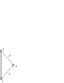
(a) Minkowski

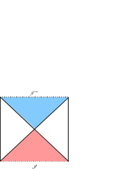
(b) dS

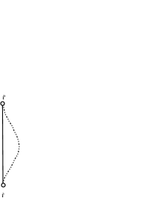
(c) AdS

Figure 1: The conformal diagrams for the maximally symmetric spacetimes: (a) Minkowski, (b) de Sitter and (c) anti-de Sitter. The double-dotted lines denote infinities, while the red and blue regions denote the future and past trapped regions, respectively. The solid lines on the boundary of these regions denote trapping horizons.

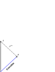
(a) Minkowski ($K=-1$)

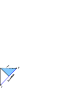
(b) dS ($K=0$)

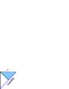
(c) dS ($K=-1$)

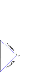
(d) AdS ($K=-1$)

Figure 2: The conformal diagrams for (a) Minkowski in the open chart, (b) de Sitter in the flat chart, (c) de Sitter in the open chart and (d) anti-de Sitter in the open chart. In all these cases, the chart covers only a part of the maximally extended spacetime.

III Flat FLRW solutions

As can be seen from Eq. (25), $a$ is a monotonic function of $t$ for $K=0$. We choose the expanding branch, the collapsing branch being the time reverse of this. Equation (24) can be integrated to give

$$a=Ct^{\frac{2}{3(1+w)}}$$ (49)

for $w>-1$ and $0<t<\infty$ or

$$a=C(-t)^{\frac{2}{3(1+w)}}$$ (50)

for $w<-1$ and $-\infty<t<0$, the constant being

$$C=[6\pi(1+w)^{2}\rho_{0}]^{\frac{1}{3(1+w)}}a_{0}\,.$$ (51)

The form of $a(t)$ is shown in Fig. 3 and we note that the gradient is infinite (zero) at $t=0$ for $w<-1$ or $-1/3<w$ ($-1<w<-1/3$). The conformal time is

$$\eta=\frac{1}{C}\frac{3(1+w)}{1+3w}t^{\frac{1+3w}{3(1+w)}}$$ (52)

for $w>-1$ (but excluding $w=-1/3$) and

$$\eta=-\frac{1}{C}\frac{3(1+w)}{1+3w}(-t)^{\frac{1+3w}{3(1+w)}}$$ (53)

for $w<-1$. Since the metric has the conformally flat form in terms of $\eta$, the conformal diagram for this spacetime is just part of the Minkowski spacetime shown in Fig. 1(a) for some appropriate domain of $\eta$ and $r$. For $w\neq-1/3$, we have

$$\frac{2m}{R}=\left(\frac{2}{1+3w}\right)^{2}\frac{r^{2}}{\eta^{2}}\,,$$ (54)

so there is a trapping horizon along

$$\eta=\pm\frac{2}{1+3w}r\,.$$ (55)

The region $r>|(1+3w)\eta|/2$ is past trapped. Note that there are just past trapped regions in this case.

The affine parameter along null geodesics is

$$\lambda=\left\{\begin{array}[]{cc}|\eta|^{\frac{5+3w}{1+3w}}&(w\neq-1/3,-1,-5/3)\\ \ln|\eta|&(w=-5/3)\\ \end{array}\right.$$ (56)

up to an affine transformation, so the affine length along null geodesics to the spacetime boundaries also depends on the value of $w$. We discuss the different cases below, summarise the spacetime boundaries in Table 1 and show the conformal diagrams in Fig. 4.

Figure 3: Evolution of the scale factor $a(t)$ for different values of $K$, $w$ and the parameter describing the solutions.

• F1: $w>-1/3$
  In this case, the domain of $\eta$ is $0<\eta<\infty$, so we have the upper half of the conformal diagram of Minkowski spacetime. $\eta=0$ corresponds to a big-bang singularity, $\eta=r=\infty$ to future null infinity and $\eta=\infty$ with $r<\infty$ to timelike infinity. The trapping horizon starts at $\eta=r=0$ and is timelike, null and spacelike for $-1/3<w<1/3$, $w=1/3$ and $w>1/3$, respectively. There is a particle horizon but no cosmological event horizon.

• F2: $w=-1/3$
  In this case, Eq. (31) with $K=0$ implies $a=\tilde{a}_{c}^{1/2}t$ for $0<t<\infty$, so the expansion speed is constant. The conformal time is $\eta=\tilde{a}_{c}^{-1/2}\ln t$ and the domain of $\eta$ is $-\infty<\eta<\infty$, so the conformal diagram is the same as that of Minkowski spacetime. $\eta=-\infty$ corresponds to a big-bang singularity, this being null. The Misner-Sharp mass is given by

  $$\frac{2m}{R}=\tilde{a}_{c}r^{2},$$ (57)

  so there is a trapping horizon at $r=\tilde{a}_{c}^{-1/2}$ and this is timelike and does not cross $r=0$. The region $r>\tilde{a}_{c}^{-1/2}$ is past trapped. There is no particle horizon or cosmological event horizon. The affine parameter along null geodesics is

  $$\lambda=e^{2\tilde{a}_{c}^{1/2}\eta}$$ (58)

  up to an affine transformation. Thus the boundary $\eta=r=\infty$ corresponds to null infinity, while the boundary $\eta=-r=-\infty$ is at a finite affine length.

• F3: $-1<w<-1/3$
  In this case, the domain of $\eta$ is $-\infty<\eta<0$, so we have the lower half of the conformal diagram of Minkowski spacetime. $\eta=0$ corresponds to future null infinity, which is spacelike, and $\eta=-\infty$ to the big-bang singularity, which is null. The trapping horizon starts at $\eta=r=0$ and is timelike. There is a cosmological event horizon but no particle horizon.

• F4: $w<-1$
  In this case, $-\infty<t<0$ is mapped to $-\infty<\eta<0$, so we again have the lower half of the conformal diagram of Minkowski spacetime. $\eta=0$ corresponds to the future big-rip singularity, which is spacelike, and $\eta=-\infty$ corresponds to $t=-\infty$. In the latter limit, there is no divergence in the curvature invariants, so $\eta=-\infty$ with $r<\infty$ corresponds to past timelike infinity. Therefore the 3-space emerges from $a=0$ without a singularity. The trapping horizon terminates at $\eta=r=0$ and is spacelike. There is a cosmological event horizon but no particle horizon. There are then three subcases.

  • F4a: $-5/3<w<-1$
    The boundaries $\eta=-\infty$ and $\eta=0$ are at finite and infinite affine lengths along null geodesics, respectively. Therefore the boundary $\eta=-r=-\infty$ is a regular null hypersurface at a finite affine length, while the boundary $\eta=0$ is a future big-rip singularity which can be reached in a finite affine length along timelike geodesics but not along null geodesics. Any null geodesic is complete in the future but incomplete in the past. This can be understood from Ref. FernandezJambrina:2006hj . Although the detailed analysis of the extension beyond the regular null hypersurface $\eta=-r=-\infty$ is beyond the scope of this paper, a possible extension may be obtained by pasting the time reverse of the solution onto this null hypersurface. This extension is at least $C^{2}$ and the conservation law (20) holds across the null hypersurface. Any null geodesic is complete in both the future and the past in this extension.

  • F4b: $w=-5/3$
    The boundaries $\eta=-\infty$ and $\eta=0$ are both at an infinite affine length along null geodesics. Therefore the boundary $\eta=-r=-\infty$ is past null infinity, while the boundary $\eta=0$ is a future big-rip singularity which can be reached in a finite affine length along timelike geodesics but not along null geodesics. Any null geodesic is complete both in the future and in the past.

  • F4c: $w<-5/3$
    The boundaries $\eta=-\infty$ and $\eta=0$ are at infinite and finite affine lengths along null geodesics, respectively. Therefore the boundary $\eta=-r=-\infty$ is past null infinity, while the boundary $\eta=0$ is a future big-rip singularity which can be reached in a finite affine length both along timelike and null geodesics. Any null geodesic is incomplete in the future but complete in the past.

Table 1: Flat FLRW solutions

		$t$	$\eta$	$a$	$\rho$	$r<\infty$	$r=\infty$
F1:	$-1/3<w<\infty$	$\infty$	$\infty$	$\infty$	$0$	$i^{+}$	$\mathscr{I}^{+}$
		$0$	$0$	$0$	$\infty$	BB	$i^{0}$
F2:	$w=-1/3$	$\infty$	$\infty$	$\infty$	$0$	$i^{+}$	$\mathscr{I}^{+}$
		$0$	$-\infty$	$0$	$\infty$	BB	BB
F3:	$-1<w<-1/3$	$\infty$	$0$	$\infty$	$0$	$\mathscr{I}^{+}$	$i^{0}$
		$0$	$-\infty$	$0$	$\infty$	BB	BB
F4a:	$-5/3<w<-1$	$0$	$0$	$\infty$	$\infty$	FBR & $\mathscr{I}^{+}$	$i^{0}$
		$-\infty$	$-\infty$	$0$	$0$	$i^{-}$	RNHS
F4b:	$w=-5/3$	$0$	$0$	$\infty$	$\infty$	FBR & $\mathscr{I}^{+}$	$i^{0}$
		$-\infty$	$-\infty$	$0$	0	$i^{-}$	$\mathscr{I}^{-}$
F4c:	$-\infty<w<-5/3$	$0$	$0$	$\infty$	$\infty$	FBR	$i^{0}$
		$-\infty$	$-\infty$	$0$	$0$	$i^{-}$	$\mathscr{I}^{-}$

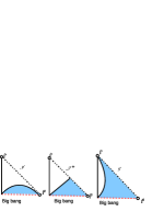
(a) F1: $w>1/3$, $w=1/3$, $-1/3<w<1/3$

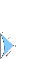
(b) F2: $w=-1/3$

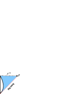
(c) F3: $-1<w<-1/3$

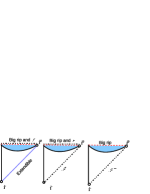
(d) F4a: $-5/3<w<-1$, F4b: $w=-5/3$, F4c: $w<-5/3$

Figure 4: The conformal diagrams for the flat FLRW solutions. The red dashed lines denote spacetime singularities, while the blue short-dashed line denotes a regular null hypersurfaces at finite affine distance. In Fig. 4(a), the left, middle and right panels correspond to $w>1/3$, $w=1/3$ and $-1/3<w<1/3$, respectively, all of which are classified as F1. Figures 4(b) and 4(c) correspond to F2 ($w=-1/3$) and F3 ($-1<w<-1/3$), respectively. In Fig. 4(d), the left, middle and right panels correspond to F4a ($-5/3<w<-1$), F4b ($w=-5/3$) and F4c ($w<-5/3$), respectively. For $-5/3\leq w<-1$, the future big-rip singularity can be reached only in an infinite affine length along null geodesics. In this sense, the future boundary of the spacetime is both a future big-rip singularity and future null infinity. This is not the case for $w<-5/3$, where null geodesics also terminate at the future big-rip singularity in a finite affine length. The boundary $t=-r=-\infty$, where $a=0$, is a regular null hypersurface at a finite affine length for $-5/3<w<-1$, beyond which the spacetime is at least $C^{2}$-extendible, while it is past null infinity for $w\leq-5/3$.

IV Positive-curvature FLRW solutions

As can be seen in Eq. (25) with $K=1$, for $w>-1/3$ the scale factor begins at zero, increases to $a_{c}$ and then decreases to zero. However, for $w<-1/3$, it begins at infinity, decreases to $a_{c}$ and then increases to infinity. For $w=-1/3$, the expansion speed is constant. More precisely, for $w\neq-1/3$, the solution of Eq. (28) with $K=1$ is

$$\tilde{a} = \tilde{a}_{c}\frac{1-\cos\tilde{\eta}}{2}\,,~{}~{}\tilde{t}=\tilde{a}_{c}\frac{\tilde{\eta}-\sin\tilde{\eta}}{2}\,,$$ (59)

where $0<\tilde{\eta}<2\pi$. The form of $a(t)$ is shown in Fig. 3. The metric is conformal to that of the Einstein static universe with the conformal time being

$$\eta=\frac{1}{1+3w}\tilde{\eta}\,.$$ (60)

A straightforward calculation gives

$$\frac{2m}{R}=\frac{\sin^{2}r}{\sin^{2}(\tilde{\eta}/2)}\,,$$ (61)

so there are two trapping horizons at

$$\eta=\frac{2}{1+3w}r\,,\quad\frac{2}{1+3w}(\pi-r)$$ (62)

and these cross each other at $(r,\eta)=(\pi/2,\pi/(1+3w))$. We note that a photon can circumnavigate the universe before it crunches for $-1/3<w<0$.

As for the affine lengths of null geodesics, we only have to focus on $\eta=0$ and $2\pi/(1+3w)$ for $w\neq-1/3,-1$. In this case, as $\eta\to 0$, we find

$$\lambda\simeq\left\{\begin{array}[]{cc}|\eta|^{\frac{5+3w}{1+3w}}&(w\neq-1/3,-1,-5/3)\\ \ln|\eta|&(w=-5/3)\\ \end{array}\right.$$ (63)

up to an affine transformation. The affine parameter in the limit $\eta\to 2\pi/(1+3w)$ corresponding to another boundary is given by replacing $\eta$ with $2\pi/(1+3w)-\eta$ in Eq. (63).

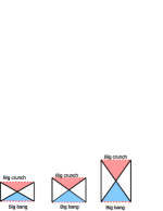
(a) P1: $w>1/3$, $w=1/3$, $-1/3<w<1/3$

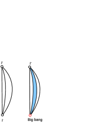
(b) P2: $w=-1/3$

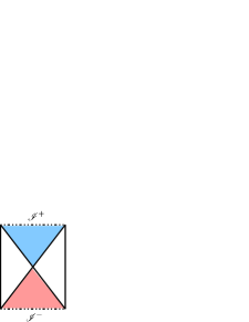
(c) P3: $-1<w<-1/3$

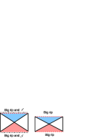
(d) P4a: $-5/3\leq w<-1$, P4b: $w<-5/3$

Figure 5: The conformal diagrams for the positive-curvature FLRW solutions. In Fig. 5(a), the left, middle and right panels correspond to $w>1/3$, $w=1/3$ and $-1/3<w<1/3$, respectively, all of which are classified as P1. In Fig. 5(b), the left and right panels correspond to $w=-1/3$ with $\tilde{a}_{c}=1$ and $\tilde{a}_{c}>1$, respectively, both of which are classified as P2. Figure 5(c) corresponds to P3 ($-1<w<-1/3$). In Fig. 5(d), the left and right panels correspond to P4a ($-5/3\leq w<-1$) and P4b ($w<-5/3$), respectively.

Table 2 summarises the spacetime boundaries and Fig. 5 shows the conformal diagrams for $K=1$. We now discuss the various cases. Note that there are both past and future trapped regions and also both particle and cosmological event horizons in this case.

• P1: $w>-1/3$
  In this case, the domain of $\eta$ is $0<\eta<2\pi/(1+3w)$. The scale factor is always smaller than or equal to $a_{c}$ and $\rho$ is a decreasing function of $a$. Therefore $\rho$ is bounded from below by its value at maximum expansion, which occurs at $\eta=\pi/(1+3w)$. Thus $\eta=0$ and $\eta=2\pi/(1+3w)$ correspond to big-bang and big-crunch singularities, respectively. The trapping horizons are spacelike for $w>1/3$, null for $w=1/3$ and timelike for $-1/3<w<1/3$. Because of the recollapsing dynamics, the region with $0<\eta<\pi/(1+3w)$ and $[(1+3w)/2]\eta<r<\pi-[(1+3w)/2]\eta$ is past trapped, while the one with $\pi/(1+3w)<\eta<2\pi/(1+3w)$ and $\pi-[(1+3w)/2]\eta<r<[(1+3w)/2]\eta$ is future trapped.

• P2: $w=-1/3$
  In this case, Eq. (31) gives two solutions. If $\tilde{a}_{c}=1$, then $a=a_{0}$ and $\eta=t/a_{0}$, where $a_{0}$ is a constant of integration. The spacetime is then identical to the Einstein static universe, with no singularity, and the domain of $\eta$ is $-\infty<\eta<\infty$. If $\tilde{a}_{c}>1$ and the expanding branch is chosen, $a=\sqrt{\tilde{a}_{c}-1}\,t$. The collapsing branch is just its time reverse. The conformal time is given by $\eta=({1}/{\sqrt{\tilde{a}_{c}-1}})\ln t\,$ and the domain of $\eta$ being $-\infty<\eta<\infty$. In both cases, the $(\eta,r)$ part of the metric is already conformally flat. However, the domain of $(\eta,r)$, which is $-\infty<\eta<\infty$ and $0\leq r\leq\pi$, is unbounded. By the transformation

  $$2\eta=\tan\left(\frac{T+X}{2}\right)+\tan\left(\frac{T-X}{2}\right),~{}~{}2r=\tan\left(\frac{T+X}{2}\right)-\tan\left(\frac{T-X}{2}\right)\,,$$ (64)

  we then obtain the following form for the metric:

  $$ds^{2} = \frac{1}{4}a^{2}(\eta)\sec^{2}\left(\frac{T+X}{2}\right)\sec^{2}\left(\frac{T-X}{2}\right)$$ (65)

  $$\times \left[-dT^{2}+dX^{2}+4\cos^{2}\left(\frac{T+X}{2}\right)\cos^{2}\left(\frac{T-X}{2}\right)\sin^{2}r\,d\Omega^{2}\right],$$

  where $\eta$ and $r$ are regarded as functions of $T$ and $X$ and the domain of $(X,T)$ is

  $$-\pi<T-X<\pi\,,~{}~{}-\pi<T+X<\pi\,,~{}~{}X\geq 0,\,~{}~{}$$

  $$\tan\left(\frac{T+X}{2}\right)-\tan\left(\frac{T-X}{2}\right)\leq 2\pi\,.$$ (66)

  $\eta=-\infty$ is transformed to $(X,T)=(0,-\pi)$, which is past timelike infinity for $\tilde{a}_{c}=1$ but a big-bang singularity for $\tilde{a}_{c}>1$. The timelike curve $r=0$ is transformed to $X=0$, while $r=\pi$ is transformed to

  $$\tan\left(\frac{T+X}{2}\right)-\tan\left(\frac{T-X}{2}\right)=2\pi\,.$$ (67)

  This can be written as

  $$T-X=2\arctan\left[\tan\left(\frac{T+X}{2}\right)-2\pi\right],$$ (68)

  which passes through $(X,T)=(2\arctan\pi,0)$, $(0,\pi)$ and $(0,-\pi)$. In this case,

  $$\frac{2m}{R}=\tilde{a}_{c}\sin^{2}r\,,$$ (69)

  so there is a trapping horizon at $r=\pi/2$, which is timelike, but no trapped region for $\tilde{a}_{c}=1$. For $\tilde{a}_{c}>1$, there are two trapping horizons at

  $$r=\arcsin(\tilde{a}_{c}^{-1/2}),~{}~{}\pi-\arcsin(\tilde{a}_{c}^{-1/2})\,.$$ (70)

  These are both timelike. The region with $\arcsin(\tilde{a}_{c}^{-1/2})<r<\pi-\arcsin(\tilde{a}_{c}^{-1/2})$ is past trapped. For $w=-1/3$, the affine parameter is

  $$\lambda = \left\{\begin{array}[]{cc}\eta&(\tilde{a}_{c}=1)\\ e^{2\sqrt{\tilde{a}_{c}-1}\eta}&(\tilde{a}_{c}>1)\end{array}\right.$$ (73)

  up to an affine transformation. Thus, for $\tilde{a}_{c}=1$, both the boundaries $\eta=\pm\infty$ are at an infinite affine length along null geodesics. For $\tilde{a}_{c}>1$, the boundaries $\eta=\infty$ and $\eta=-\infty$ are at infinite and finite affine lengths along null geodesics, respectively.

• P3: $-1<w<-1/3$
  In this case, the scale factor is never less than $a_{c}$ and $\rho$ is a decreasing function of $a$. Therefore $\rho$ is bounded from above by the value at the bounce, which occurs at $\eta=\pi/(1+3w)$. The domain of $\eta$ is $2\pi/(1+3w)<\eta<0$, with $\eta=0$ and $2\pi/(1+3w)$ corresponding to null infinities rather than singularities. The trapping horizons are timelike. Because of the bouncing dynamics, the region with $\pi/(1+3w)<\eta<0$ and $[(1+3w)/2]\eta<r<\pi-[(1+3w)/2]\eta$ is past trapped, while that with $2\pi/(1+3w)<\eta<\pi/(1+3w)$ and $\pi-[(1+3w)/2]\eta<r<[(1+3w)/2]\eta$ is future trapped.

• P4: $w<-1$
  In this case, the scale factor is never less than $a_{c}$ and the energy density is an increasing function of $a$. The domain of $\eta$ is $2\pi/(1+3w)<\eta<0$, with $\eta=2\pi/(1+w)$ and $0$ corresponding to past and future big-rip singularities, respectively. The bounce occurs at $\eta=\pi/(1+3w)$, where $\rho$ reaches its minimum. The trapping horizons are spacelike. Because of the bouncing dynamics, the region with $\pi/(1+3w)<\eta<0$ and $[(1+3w)/2]\eta<r<\pi-[(1+3w)/2]\eta$ is past trapped, while that with $2\pi/(1+3w)<\eta<\pi/(1+3w)$ and $\pi-[(1+3w)/2]\eta<r<[(1+3w)/2]\eta$ is future trapped. There are then two subcases.

  • P4a: $-5/3\leq w<-1$
    The boundaries $\eta=2\pi/(1+3w)$ and $\eta=0$ are both null infinities. Therefore they are both big-rip singularities and null infinities, simultaneously.

  • P4b: $w<-5/3$
    The boundaries $\eta=2\pi/(1+3w)$ and $\eta=0$ are both at a finite affine length. Therefore they are big-rip singularities but not null infinities.

Table 2: Positive-curvature FLRW solutions

		$t$	$\tilde{t}$	$\eta$	$\tilde{\eta}$	$a$	$\tilde{a}$	$\rho$	$r<\infty$
P1:	$-1/3<w<\infty$	$t_{0}$	$\pi\tilde{a}_{c}$	$2\pi/(1+3w)$	$2\pi$	$0$	$0$	$\infty$	BC
		$0$	$0$	$0$	$0$	$0$	$0$	$\infty$	BB
P2:	$w=-1/3$ ($\tilde{a}_{c}=1$)	$\infty$	–	$\infty$	–	$a_{0}$	–	$\rho_{0}$	$i^{+}$
		$-\infty$	–	$\infty$	–	$a_{0}$	–	$\rho_{0}$	$i^{-}$
P2:	$w=-1/3$ ($\tilde{a}_{c}>1$)	$\infty$	–	$\infty$	–	$\infty$	–	$0$	$i^{+}$
		$0$	–	$-\infty$	–	$0$	–	$\infty$	BB
P3:	$-1<w<-1/3$	$\infty$	$0$	$0$	$0$	$\infty$	$0$	$0$	$\mathscr{I}^{+}$
		$-\infty$	$\pi\tilde{a}_{c}$	$2\pi/(1+3w)$	$2\pi$	$\infty$	$0$	$0$	$\mathscr{I}^{-}$
P4a:	$-5/3\leq w<-1$	$t_{0}$	$0$	$0$	$0$	$\infty$	$0$	$\infty$	FBR  & $\mathscr{I}^{+}$
		$0$	$\pi\tilde{a}_{c}$	$2\pi/(1+3w)$	$2\pi$	$\infty$	$0$	$\infty$	PBR  & $\mathscr{I}^{-}$
P4b:	$-\infty<w<-5/3$	$t_{0}$	$0$	$0$	$0$	$\infty$	$0$	$\infty$	FBR
		$0$	$\pi\tilde{a}_{c}$	$2\pi/(1+3w)$	$2\pi$	$\infty$	$0$	$\infty$	PBR

V Negative-curvature FLRW solutions

For $K=-1$, the conformally static form of the metric (12) can be written as Sato:1996

$$ds^{2}=a^{2}(\eta)\frac{-d\eta^{\prime 2}+dr^{\prime 2}+\sin^{2}r^{\prime}d\Omega^{2}}{\cos(r^{\prime}+\eta^{\prime})\cos(r^{\prime}-\eta^{\prime})}\,,$$ (74)

where

$$\tan\eta^{\prime}=\frac{\sinh\eta}{\cosh r}\,,~{}~{}\tan r^{\prime}=\frac{\sinh r}{\cosh\eta}\,.$$ (75)

Therefore the metric is conformal to the Einstein static universe. In this case – and only this case – the energy density can be negative, so we consider this possibility below.

V.1 Vacuum

For pedagogical completeness, we consider the vacuum case, in which the solution is part of Minkowski spacetime. The Friedmann equation with $\rho=0$ and $K=-1$ gives $a=t$ with $0<t<\infty$ for the expanding branch, corresponding to the Milne universe. The collapsing branch is the time reverse of this. Since $\eta=\ln t,$ the domain $0<t<\infty$ is mapped to $-\infty<\eta<\infty$. In the form which is conformal to the Einstein static universe, the domain of $\eta^{\prime}$ and $r^{\prime}$ is the intersection of $-\pi/2<\eta^{\prime}<\pi/2$, $0\leq r^{\prime}<\pi/2$, $-\pi/2<r^{\prime}-\eta^{\prime}<\pi/2$ and $-\pi/2<r^{\prime}+\eta^{\prime}<\pi/2$. The affine parameter along null geodesics is given by $\lambda=e^{2\eta}$ up to an affine transformation. Therefore, the past boundary $t=0$ or $\eta=-\infty$ is at a finite affine length along null geodesics. As it is well known, the metric can be transformed to the standard Minkowski form with the substitution $T=t\cosh r$ and $X=t\sinh r$. While the domain of $T$ and $X$ is originally the intersection of $0<T<\infty$, $0\leq X<\infty$ and $T>X$, it can be maximally extended beyond $T=X$ to the region $-\infty<T<\infty$ and $0\leq X<\infty$. The past boundaries $\{t=0,\,r<\infty\}$ and $\{t=0,\,r=\infty\}$ of the Milne universe are transformed to the point $T=X=0$ and the null hypersurface $T=X$, respectively. We will see below that this extension is also possible for $\rho\neq 0$ and $w<-1$. Table 3 summarises the spacetime boundaries and Fig. 6 shows the conformal diagram of the Milne universe.

Table 3: Negative-curvature vacuum FLRW solution or the Milne universe

	$t$	$\eta$	$a$	$\rho$	$r<\infty$	$r=\infty$
Milne	$\infty$	$\infty$	$\infty$	$0$	$i^{+}$	$\mathscr{I}^{+}$
	$0$	$-\infty$	$0$	$0$	regular	RNHS

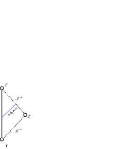
Figure 6: The conformal diagram for the negative-curvature FLRW solution or the Milne universe is shown as part of the Minkowski spacetime, which is its maximal extension.

V.2 Positive energy density

If $\rho$ is positive, Eq. (19) shows that the scale factor $a$ is a monotonic function of $t$. For the expanding solution, it begins at $0$ at a finite value of $t$ and then increases to $\infty$ as $t$ increases. More precisely, for $w\neq-1/3$, the expanding solution of Eq. (28) with $K=-1$ is given by

$$\tilde{a} = \tilde{a}_{c}\frac{\cosh\tilde{\eta}-1}{2}\,,~{}~{}\tilde{t}=\tilde{a}_{c}\frac{\sinh\tilde{\eta}-\tilde{\eta}}{2}\,,$$ (76)

where $0<\tilde{\eta}<\infty$ and $\tilde{\eta}$ is related to $\eta$ by

$$\eta=\frac{1}{1+3w}\tilde{\eta}\,.$$ (77)

The collapsing solution is the time reverse of this. The form of $a(t)$ is shown in Fig. 3. The Misner-Sharp mass is given by

$$\frac{2m}{R}=\frac{\sinh^{2}r}{\sinh^{2}(\tilde{\eta}/{2})}\,,$$ (78)

so there is a trapping horizon at

$$\eta=\frac{2}{1+3w}r\,.$$ (79)

This is spacelike for $w>1/3$ and $w<-1$, null for $w=1/3$ and timelike for $-1/3<w<1/3$. The region $r>|(1+3w)\eta|/2$ is past trapped.

As for the affine lengths of null geodesics, for $\eta\to 0$ we find the behaviour of the affine parameter is the same as in the positive curvature case and given by Eq. (63) up to an affine transformation. For $w\neq-1/3$, the affine parameter along null geodesics for $\eta\to\pm\infty$ is as follows:

$$\lambda\simeq\left\{\begin{array}[]{cc}e^{2|\eta|}&(w>-1/3)\\ e^{-2|\eta|}&(w<-1/3)\\ \end{array}\right.$$ (80)

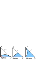
(a) NP1: $w>1/3$, $w=1/3$, $-1/3<w<1/3$

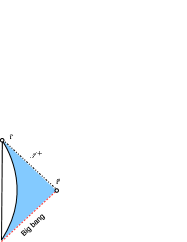
(b) NP2: $w=-1/3$

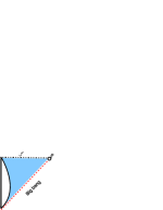
(c) NP3: $-1<w<-1/3$

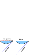
(d) NP4a: $-5/3\leq w<-1$, NP4b: $w<-5/3$

Figure 7: The conformal diagrams for the negative-curvature FLRW solutions with a positive energy density. In Fig. 7(a), the left, middle and right panels correspond to $w>1/3$, $w=1/3$ and $-1/3<w<1/3$, respectively, all of which are classified as NP1. Figures 7(b) and 7(c) correspond to NP2 ($w=-1/3$) and NP3 ($-1<w<-1/3$), respectively. In Fig. 7(d), the left and right panels correspond to NP4a ($-5/3\leq w<-1$) and NP4b ($w<-5/3$), respectively. The blue short-dashed lines for $w<-1$ are regular null hypersurfaces at finite affine lengths, beyond which the spacetime is at least $C^{2}$-extendible.

up to an affine transformation. Table 4 summarises the spacetime boundaries and Fig. 7 shows the conformal diagrams for $K=-1$ with a positive energy density. Figure 7 looks almost identical to Fig. 4 but is very different in the past boundaries for $w<-1$. We now discuss the various cases.

• NP1: $w>-1/3$
  In this case, $\dot{a}\to 1$ as $a\to\infty$, corresponding to infinity at $t=\infty$ or $\eta=\infty$ rather than a big-rip singularity. However, $t=0$ or $\eta=0$ corresponds to a big-bang singularity. The domain of $\eta$ and $r$ is $0<\eta<\infty$ and $0\leq r<\infty$, this being mapped to $0<\eta^{\prime}<\pi/2$, $0\leq r^{\prime}<\pi/2$ and $\eta^{\prime}+r^{\prime}<\pi/2$. The big-bang singularity at $\eta=0$ is mapped to $\eta^{\prime}=0$. The boundary $\eta=\infty$ with $r<\infty$ is mapped to $(r^{\prime},\eta^{\prime})=(0,\pi/2)$, corresponding to future timelike infinity. The boundary $r=\infty$ with $\eta<\infty$ is mapped to $(r^{\prime},\eta^{\prime})=(\pi/2,0)$, corresponding to spatial infinity. The boundary $\eta=r=\infty$ is mapped to $\eta^{\prime}+r^{\prime}=\pi/2$, corresponding to future null infinity. The trapping horizon starts at $\eta^{\prime}=r^{\prime}=0$. There is a particle horizon but no cosmological event horizon.

• NP2: $w=-1/3$
  In this case, the Friedmann equation gives $a=\sqrt{\tilde{a}_{c}+1}\,t,$ where $0<t<\infty$ and the expanding branch is chosen. The collapsing one is the time reverse of this. Since $\eta=(1/\sqrt{\tilde{a}_{c}+1})\ln t,$ the domain of $\eta$ is $-\infty<\eta<\infty$, where $\eta=-\infty$ corresponds to the big-bang singularity. In this case

  $$\frac{2m}{R}=\tilde{a}_{c}\sinh^{2}r,$$ (81)

  so there is a trapping horizon at $r=\mbox{arcsinh}(\tilde{a}_{c}^{-1/2})\,,$ which is timelike. The region $r>\mbox{arcsinh}(\tilde{a}_{c}^{-1/2})$ is past trapped. There is no particle horizon or cosmological event horizon. The affine parameter is given by

  $$\lambda=e^{2\sqrt{\tilde{a}_{c}+1}\eta}$$ (82)

  up to an affine transformation. Thus the boundary $\eta=r=\infty$ corresponds to null infinity, while the boundary $\eta=-r=-\infty$ is at a finite affine length.

• NP3: $-1<w<-1/3$
  In this case, as $a\to\infty$, the curvature term becomes subdominant in the Friedmann equation and so the solution asymptotically approaches the flat model. The domain of $\eta$ and $r$ is $-\infty<\eta<0$ and $0\leq r<\infty$, this being mapped to $-\pi/2<\eta^{\prime}<0$, $0\leq r^{\prime}<\pi/2$ and $\eta^{\prime}-r^{\prime}>-\pi/2$. The boundary $\eta=0$ is mapped to $\eta^{\prime}=0$, corresponding to future null infinity. The boundary $\eta=-\infty$ with $r<\infty$ is mapped to $(r^{\prime},\eta^{\prime})=(0,-\pi/2)$, corresponding to a big-bang singularity. The boundary $r=\infty$ with $\eta<\infty$ is mapped to $(r^{\prime},\eta^{\prime})=(\pi/2,0)$, corresponding to spatial infinity. The boundary $-\eta=r=\infty$ is mapped to $\eta^{\prime}-r^{\prime}=-\pi/2$, corresponding to a big-bang singularity. The trapping horizon terminates at $\eta^{\prime}=r^{\prime}=0$. There is no particle horizon but a cosmological event horizon.

• NP4: $w<-1$
  In this case, as $a$ increases, the Friedmann equation is dominated by the density term and the solution ends with a future big-rip singularity at a finite value of $t$. This can be seen from Eqs. (27) and (76). As $a$ decreases, the density term becomes subdominant compared to the curvature term. The scale factor $a$ vanishes at $t=0$, with $\dot{a}$ approaching unity and the curvature invariants vanishing in this limit. This implies that the solution approaches the Milne universe as $t\to 0$ and is extendible beyond the $t=0$ null hypersurface. The domain of $\eta$ and $r$ is $-\infty<\eta<0$ and $0\leq r<\infty$. This is mapped to the intersection of $-\pi/2<\eta^{\prime}<0$, $0\leq r^{\prime}<\pi/2$ and $\eta^{\prime}-r^{\prime}>-\pi/2$. The conformal diagram is similar to the NP2 case, except that $\eta^{\prime}=0$ corresponds to a future big-rip singularity, while $\eta^{\prime}-r^{\prime}=-\pi/2$ corresponds to a regular null hypersurface, which is $C^{2}$-extendible to Minkowski spacetime. However, note that $\rho_{0}$ in Eq. (23) must be constant in the whole spacetime to ensure the conservation law (20). Since $\rho_{0}$ trivially vanishes in Minkowski spacetime, the $C^{2}$-extension to Minkowski breaks the conservation law across the null hypersurface. The trapping horizon terminates at $\eta^{\prime}=r^{\prime}=0$ and is spacelike. There is a cosmological event horizon but no particle horizon. There are then two subcases.

  • NP4a: $-5/3\leq w<-1$
    In this case, $\eta=0$ corresponds to future null infinity, while $\eta=-\infty$ is at a finite affine length. The boundary $\eta=0$ is both a future big-rip singularity and future null infinity.

  • NP4b: $w<-5/3$
    In this case, the boundaries $\eta=0$ and $\eta=-\infty$ are both at finite affine lengths. The boundary $\eta=0$ is a future big-rip singularity but not future null infinity.

Table 4: Negative-curvature FLRW solutions with $\rho>0$

		$t$	$\tilde{t}$	$\eta$	$\tilde{\eta}$	$\eta^{\prime}$	$a$	$\tilde{a}$	$\rho$	$r<\infty$	$r=\infty$
NP1:	$-1/3<w<\infty$	$\infty$	$\infty$	$\infty$	$\infty$	$\pi/2$	$\infty$	$\infty$	$0$	$i^{+}$	$\mathscr{I}^{+}$
		$0$	$0$	$0$	$0$	$0$	$0$	$0$	$\infty$	BB	$i^{0}$
NP2:	$w=-1/3$	$\infty$	–	$\infty$	–	–	$\infty$	–	$0$	$i^{+}$	$\mathscr{I}^{+}$
		$0$	–	$-\infty$	–	–	$0$	–	$\infty$	BB	BB
NP3:	$-1<w<-1/3$	$\infty$	$0$	$0$	$0$	$0$	$\infty$	$0$	$0$	$\mathscr{I}^{+}$	$i^{0}$
		$0$	$\infty$	$-\infty$	$\infty$	$-\pi/2$	$0$	$\infty$	$\infty$	BB	BB
NP4a	$-5/3\leq w<-1$	$t_{0}$	$0$	$0$	$0$	$0$	$\infty$	$0$	$\infty$	FBR  & $\mathscr{I}^{+}$	$i^{0}$
		$0$	$\infty$	$-\infty$	$\infty$	$-\pi/2$	$0$	$\infty$	$0$	regular	RNHS
NP4b:	$-\infty<w<-5/3$	$t_{0}$	$0$	$0$	$0$	$0$	$\infty$	$0$	$\infty$	FBR	$i^{0}$
		$0$	$\infty$	$-\infty$	$\infty$	$-\pi/2$	$0$	$\infty$	$0$	regular	RNHS

V.3 Negative energy density

For $\rho<0$ and $w>-1/3$, the Friedmann equation implies that $a$ begins at $\infty$, decreases to $a^{\prime}_{c}:=(-\tilde{a}_{c})^{1/(1+3w)}$ and then increases to $\infty$. For $w<-1/3$, it begins at $0$, increases to $a^{\prime}_{c}$ and then decreases to $0$. More precisely, for $w\neq-1/3$, integrating Eq. (28) gives

$$\tilde{a} = \tilde{a}^{\prime}_{c}\frac{1+\cosh\tilde{\eta}}{2},~{}~{}\tilde{t}=\tilde{a}^{\prime}_{c}\frac{\tilde{\eta}+\sinh\tilde{\eta}}{2}\,,$$ (83)

where $\tilde{a}_{c}^{\prime}=-\tilde{a}_{c}$, $-\infty<\tilde{\eta}<\infty$ and the conformal time is

$$\eta=\frac{1}{1+3w}\tilde{\eta}\,.$$ (84)

For $\tilde{\eta}\to\pm\infty$, we have $\tilde{a}\to\infty$, with $\tilde{a}$ bouncing from contraction to expansion at $\tilde{a}^{\prime}_{c}$ and $\tilde{\eta}=0$. The form of $a(t)$ is shown in Fig. 3. The Misner-Sharp mass $m$ is negative if the energy density is negative. Since one always has $2m/R<1$ in this case, as seen from

$$\frac{2m}{R}=-\frac{\sinh^{2}r}{\cosh^{2}(\tilde{\eta}/{2})}\,,$$ (85)

there are no trapped or marginally trapped spheres.

For $w\neq-1/3$, the affine parameter along null geodesics for $\eta\to\pm\infty$ is also given by Eq. (80) up to an affine transformation. The spacetime boundaries are summarised in Table. 5 and the conformal diagrams shown in Fig. 8 for these cases. We now discuss the various possibilities. Note that there are no trapped regions in this case and that there is no particle horizon or cosmological event horizon.

• NN1: $w>-1/3$
  In this case, the boundaries $\eta=\pm\infty$ correspond to $a=\infty$. Equations (27) and (83) imply that these boundaries correspond to infinities at $t=\pm\infty$. The boundaries $\eta=r=\infty$ and $-\eta=r=\infty$ are future and past null infinities, respectively, while $\eta=\infty$ and $\eta=-\infty$ with $r<\infty$ are future and past timelike infinities, respectively. $r=\infty$ with $|\eta|<\infty$ corresponds to spatial infinity. There is no singularity and the spacetime is geodesically complete.

• NN2: $w=-1/3$
  In this case, from Eq. (31), we have $0\leq\tilde{a}^{\prime}_{c}\leq 1$, with $\tilde{a}^{\prime}_{c}=0$ reducing to the vacuum case. For $0<\tilde{a}^{\prime}_{c}<1$, the Friedmann equation gives the expanding solution $a=\sqrt{1-\tilde{a}^{\prime}_{c}}\,t,$ for $0<t<\infty$. The collapsing branch is just the time reverse of this. The conformal time is $\eta=({1}/{\sqrt{1-\tilde{a}^{\prime}_{c}}})\ln t,$ so $-\infty<\eta<\infty$ and $t=0$ or $\eta=-\infty$ corresponds to a big-bang singularity. For $\tilde{a}_{c}^{\prime}=1$, $a=a_{0}$ (constant) and the resulting metric is a static spatially negative-curvature universe. The conformal time is $\eta=t/a_{0}$, so $-\infty<\eta<\infty$ and this is conformal to the Einstein static model. There is no singularity and

  $$\frac{2m}{R}=-\tilde{a}^{\prime}_{c}\sinh^{2}r\,.$$ (86)

  This is always negative, so there are no trapped regions. The affine parameter along null geodesics is

  $$\lambda=\left\{\begin{array}[]{cc}e^{2\sqrt{1-\tilde{a}_{c}^{\prime}}\eta}&(0<\tilde{a}_{c}^{\prime}<1)\\ \eta&(\tilde{a}_{c}^{\prime}=1)\end{array}\right.$$ (87)

  up to an affine transformation. Therefore, for $0<\tilde{a}_{c}^{\prime}<1$, $\eta=\infty$ and $\eta=-\infty$ correspond to null infinity and the boundary at a finite affine length, respectively, while for $\tilde{a}_{c}^{\prime}=1$, the boundaries $\eta=\pm r=\pm\infty$ correspond to null infinities.

• NN3: $-1<w<-1/3$
  In this case, the boundaries $\eta=\pm\infty$ correspond to $a=0$. Equations (27) and (83) imply that $\eta=\infty$ and $\eta=-\infty$ correspond to $t=0$ and $t=t_{0}$, respectively, where $0<t_{0}<\infty$. The energy density $\rho$ diverges at $t=0$ and $t=t_{0}$, implying big-bang and big-crunch singularities, respectively. These singularities are null.

• NN4: $w<-1$
  In this case, the boundaries $\eta=\pm\infty$ correspond to $a=0$. Equations (27) and (83) imply that they correspond to $t=0$ and $t=t_{0}$, respectively, where $0<t_{0}<\infty$. The energy density vanishes both at $t=0$ and $t=t_{0}$. The Friedmann equation is dominated by the curvature term, so it asymptotically approaches the Milne one. There is no divergence in the curvature invariants, which vanish at both $t=0$ and $t=t_{0}$. Thus $\eta=\pm\infty$ correspond to regular null hypersurfaces at finite affine lengths. The spacetime is $C^{2}$-extendible to Minkowski spacetime beyond the regular null hypersurfaces.

Table 5: Negative-curvature FLRW solutions with $\rho<0$

		$t$	$\tilde{t}$	$\eta$	$\tilde{\eta}$	$\eta^{\prime}$	$a$	$\tilde{a}$	$\rho$	$r<\infty$	$r=\infty$
NN1:	$-1/3<w<\infty$	$\infty$	$\infty$	$\infty$	$\infty$	$\pi/2$	$\infty$	$\infty$	$0$	$i^{+}$	$\mathscr{I}^{+}$
		$-\infty$	$-\infty$	$-\infty$	$-\infty$	$-\pi/2$	$\infty$	$\infty$	$0$	$i^{-}$	$\mathscr{I}^{-}$
NN2:	$w=-1/3$ ($0<\tilde{a}_{c}^{\prime}<1$)	$\infty$	–	$\infty$	–	$\pi/2$	$\infty$	–	$0$	$i^{+}$	$\mathscr{I}^{+}$
		$0$	–	$-\infty$	–	$-\pi/2$	$0$	–	$\infty$	BB	BB
NN2:	$w=-1/3$ ($\tilde{a}_{c}^{\prime}=1$)	$\infty$	–	$\infty$	–	$\pi/2$	$a_{0}$	–	$\rho_{0}$	$i^{+}$	$\mathscr{I}^{+}$
		$-\infty$	–	$-\infty$	–	$-\pi/2$	$a_{0}$	–	$\rho_{0}$	$i^{-}$	$\mathscr{I}^{-}$
NN3:	$-1<w<-1/3$	$t_{0}$	$-\infty$	$\infty$	$-\infty$	$\pi/2$	$0$	$\infty$	$\infty$	BC	BC
		$0$	$\infty$	$-\infty$	$\infty$	$-\pi/2$	$0$	$\infty$	$\infty$	BB	BB
NN4:	$-\infty<w<-1$	$t_{0}$	$-\infty$	$\infty$	$-\infty$	$\pi/2$	$0$	$\infty$	$0$	regular	RNHS
		$0$	$\infty$	$-\infty$	$\infty$	$-\pi/2$	$0$	$\infty$	$0$	regular	RNHS

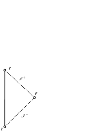
(a) NN1: $w>-1/3$

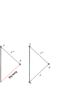
(b) NN2: $w=-1/3$

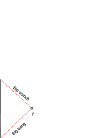
(c) NN3: $-1<w<-1/3$

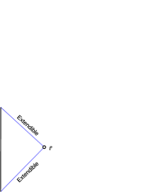
(d) NN4: $w<-1$

Figure 8: The conformal diagrams for the negative-curvature FLRW solutions with a negative energy density. There are no trapped regions in this case. Figure 8(a) corresponds to NN1 ($w>-1/3$). Figure 8(b) corresponds to NN2 ($w=-1/3$) with the left and right panels applying for $0<\tilde{a}^{\prime}_{c}<1$ and $\tilde{a}^{\prime}_{c}=1$, respectively. Figures 8(c) and 8(d) correspond to NN3 ($-1<w<-1/3$) and NN4 ($w<-1$), respectively. The blue short-dashed lines for $w<-1$ denote regular null hypersurfaces at finite affine lengths, beyond which the spacetime is at least $C^{2}$-extendible.

VI Conclusions

We have completely classified the FLRW solutions of the Einstein equation with the equation of state $p=w\rho$ according to their conformal structure, going beyond the usual energy conditions. We have classified the cases in terms of the spatial curvature $K$, the equation of state parameter $w$ and the sign of the energy density $\rho$. For the vacuum case, the FLRW solution is Minkowski spacetime, while for $w=-1$ it is the de Sitter spacetime for $\rho>0$ and the anti-de Sitter spacetime for $\rho<0$. For other cases, there is a rich variety of structures.

The important features are as follows: For each spatial curvature, the causal nature of the spacetime is the same for $w>-1/3$, as is well known. For $w=-1/3$, the speed of the cosmological expansion is constant. For $-1<w<-1/3$, there is a null big-bang singularity for $K=0$ and $-1$, but the solution describes a bouncing universe for $K=1$. For $w<-1$, the causal structure is rather exotic. For $w<-1$ and $K=0$, the universe gradually expands from a vanishing scale factor for an infinitely long time and ends with a future big-rip singularity. For $w<-1$ and $K=1$, the universe begins with a past big-rip singularity, contracts, bounces and ends with a future big-rip singularity. For $w<-1$, $K=-1$ and $\rho>0$, the universe emerges from a regular null hypersurface and ends with a future big-rip singularity. For $-5/3\leq w<-1$, null geodesics cannot reach the future big-rip singularity within a finite affine length, while for $w<-5/3$, they can. A negative energy density is only possible for $K=-1$, which describes a bouncing universe with future and past null infinities for $w>-1/3$, a universe beginning with a big-bang singularity and ending with a big-crunch singularity for $-1<w<-1/3$, and a universe emerging from a regular null hypersuface and then submerging into another regular hypersurface for $w<-1$. In general, the big-bang and past big-rip singularities are followed by past and future trapping horizons, respectively, while the big-crunch and future big-rip singularities are preceded by future and past trapping horizons, respectively.

Although we have focused on the linear equation of state, the generalisation to other types of matter fields is interesting. In particular, it is important to include both a perfect fluid and a positive or negative cosmological constant, not only in the context of classification of singularities in FLRW spacetimes but also from the cosmological point of view. Since the dominant term on the right-hand side of the Friedmann equation should determine the properties of the spacetime boundaries, the structure of big-bang singularities for $w>-1/3$ and that of big-rip singularities for $w<-1$ are unchanged even in the presence of a cosmological constant, although the intermediate dynamics of the scale factor can be greatly changed. In another paper CHI , we expand our analysis to derive the conformal diagrams for solutions which represent black holes, wormholes and baby universes in a cosmological background.

- (1) I. Zlatev, L. M. Wang and P. J. Steinhardt, “Quintessence, cosmic coincidence, and the cosmological constant,” Phys. Rev. Lett. 82 (1999) 896 doi:10.1103/PhysRevLett.82.896 [astro-ph/9807002].
- (2) R. R. Caldwell, “A Phantom menace?,” Phys. Lett. B 545 (2002) 23 doi:10.1016/S0370-2693(02)02589-3 [astro-ph/9908168].
- (3) P. Creminelli, A. Nicolis and E. Trincherini, “Galilean Genesis: An Alternative to inflation,” JCAP 1011 (2010) 021 doi:10.1088/1475-7516/2010/11/021 [arXiv:1007.0027 [hep-th]].
- (4) R. R. Caldwell, M. Kamionkowski and N. N. Weinberg, “Phantom energy and cosmic doomsday,” Phys. Rev. Lett. 91 (2003) 071301 doi:10.1103/PhysRevLett.91.071301 [astro-ph/0302506].
- (5) M. P. Dabrowski, T. Stachowiak and M. Szydlowski, “Phantom cosmologies,” Phys. Rev. D 68 (2003) 103519 doi:10.1103/PhysRevD.68.103519 [hep-th/0307128].
- (6) M. P. Dabrowski and T. Stachowiak, “Phantom Friedmann cosmologies and higher-order characteristics of expansion,” Annals Phys. 321 (2006) 771 doi:10.1016/j.aop.2005.10.006 [hep-th/0411199].
- (7) T. Chiba, R. Takahashi and N. Sugiyama, “Classifying the future of Universes with dark energy,” Class. Quant. Grav. 22 (2005) 3745 doi:10.1088/0264-9381/22/17/023 [astro-ph/0501661].
- (8) L. Fernández-Jambrina and R. Lazkoz, “Classification of cosmological milestones,” Phys. Rev. D 74 (2006) 064030 doi:10.1103/PhysRevD.74.064030 [gr-qc/0607073].
- (9) R. J. Nemiroff, R. Joshi and B. R. Patla, “An exposition on Friedmann Cosmology with Negative Energy Densities,” JCAP 1506 (2015) 006 doi:10.1088/1475-7516/2015/06/006 [arXiv:1402.4522 [astro-ph.CO]].
- (10) R. M. Wald, “General Relativity,” Chicago, USA: Univ. Pr. (1984) 491p doi:10.7208/chicago/9780226870373.001.0001.
- (11) T. M. C. Abbott et al. [DES Collaboration], “Dark Energy Survey Year 1 Results: Cosmological Constraints from Galaxy Clustering and Weak Lensing,” arXiv:1708.01530 [astro-ph.CO].
- (12) T. Harada and B. J. Carr, “Upper limits on the size of a primordial black hole,” Phys. Rev. D 71 (2005) 104009 doi:10.1103/PhysRevD.71.104009 [astro-ph/0412134].
- (13) H. Sato and H. Kodama, “Ippansoutaiseiriron: 2nd ed.” (in Japanese), (Iwanami Shoten, Publishers, Tokyo, 1996)
- (14) J. M. M. Senovilla, “Singularity Theorems and Their Consequences”, Gen. Relativ. Grav. 30 701 (1998).
- (15) J. R. Oppenheimer and H. Snyder, “On Continued gravitational contraction,” Phys. Rev. 56 (1939) 455. doi:10.1103/PhysRev.56.455.
- (16) B. J. Carr, “The Primordial black hole mass spectrum,” Astrophys. J. 201 (1975) 1. doi:10.1086/153853.
- (17) T. Harada, C. M. Yoo and K. Kohri, “Threshold of primordial black hole formation,” Phys. Rev. D 88 (2013) no.8, 084051 Erratum: [Phys. Rev. D 89 (2014) no.2, 029903] doi:10.1103/PhysRevD.88.084051, 10.1103/PhysRevD.89.029903 [arXiv:1309.4201 [astro-ph.CO]].
- (18) F. C. Mena and J. M. Oliveira, “Radiative gravitational collapse to spherical, toroidal and higher genus black holes,” Annals Phys. 387 (2017) 135 doi:10.1016/j.aop.2017.10.012 [arXiv:1710.03721 [gr-qc]].
- (19) B. J. Carr and T. Harada, “Separate universe problem: 40 years on,” Phys. Rev. D 91 (2015) no.8, 084048 doi:10.1103/PhysRevD.91.084048 [arXiv:1405.3624 [astro-ph.CO]].
- (20) M. Kopp, S. Hofmann and J. Weller, “Separate Universes Do Not Constrain Primordial Black Hole Formation,” Phys. Rev. D 83 (2011) 124025 doi:10.1103/PhysRevD.83.124025 [arXiv:1012.4369 [astro-ph.CO]].
- (21) T. Harada and B. J. Carr, “Super-horizon primordial black holes,” Phys. Rev. D 72 (2005) 044021 doi:10.1103/PhysRevD.72.044021 [astro-ph/0508122].
- (22) H. Deng, J. Garriga and A. Vilenkin, “Primordial black hole and wormhole formation by domain walls,” JCAP 1704 (2017) no.04, 050 doi:10.1088/1475-7516/2017/04/050 [arXiv:1612.03753 [gr-qc]].
- (23) J. Garriga, A. Vilenkin and J. Zhang, “Black holes and the multiverse,” JCAP 1602 (2016) no.02, 064 doi:10.1088/1475-7516/2016/02/064 [arXiv:1512.01819 [hep-th]].
- (24) K. i. Nakao, “On a quasilocal energy outside the cosmological horizon,” gr-qc/9507022.
- (25) B. J. Carr, T. Harada, T. Igata and T. Kokubu, in preparation.
- (26) S. A. Hayward, “Gravitational energy in spherical symmetry,” Phys. Rev. D 53 (1996) 1938 doi:10.1103/PhysRevD.53.1938 [gr-qc/9408002].