Isobaric Multiplet Mass Equation within nuclear Density Functional Theory

Abstract

We extend the nuclear Density Functional Theory (DFT) by including proton-neutron mixing and contact isospin-symmetry-breaking (ISB) terms up to next-to-leading order (NLO). Within this formalism, we perform systematic study of the nuclear mirror and triple displacement energies, or equivalently of the Isobaric Multiplet Mass Equation (IMME) coefficients. By comparing results with those obtained within the existing Green Function Monte Carlo (GFMC) calculations, we address the fundamental question of the physical origin of the ISB effects. This we achieve by analyzing separate contributions to IMME coefficients coming from the electromagnetic and nuclear ISB terms. We show that the ISB DFT and GFMC results agree reasonably well, and that they describe experimental data with a comparable quality. Since the separate electromagnetic and nuclear ISB contributions also agree, we conclude that the beyond-mean-field electromagnetic effects may not play a dominant role in describing the ISB effects in finite nuclei.

Similarity between the neutron-neutron, proton-proton, and proton-neutron nuclear interactions was well recognized already in the third decade of the last century. This property motivated Heisenberg [1] and Wigner [2] to introduce the concept of isospin symmetry, which abandons notions of protons and neutrons and replaces them by that of a nucleon, that is, a particle having two independent states in an abstract space called isotopic-spin space or, in short, the isospace.

The isospin symmetry is not an exact symmetry of nature. At the fundamental level, it is violated by the difference in masses of the constituent $up$ and $down$ quarks and the difference in their electric charges. At the many-body level, where nucleons are treated as structureless point-like particles interacting via the effective forces, the major source of the isospin symmetry breaking (ISB) is the Coulomb field. The strong-force ISB components are much weaker than the symmetry conserving, isoscalar ones. Nevertheless, they are firmly established from the two-body scattering data, which indicate that the neutron-neutron interaction is $\sim$1% stronger than the proton-proton one, and that the neutron-proton interaction is $\sim$2.5% stronger than the average of the former two [3].

Following the classification introduced by Henley and Miller [4, 5], components of the nuclear force can be divided into four classes that have different structures with respect to the isospin symmetry. Apart from the dominant class-I isoscalar (isospin-invariant) forces, the classification introduces three different classes of the ISB forces, namely, class-II isotensor forces, which break the isospin symmetry but are invariant under a rotation by $\pi$ with respect to the $y-$axis in the isospace; class-III isovector forces that break the isospin symmetry but are symmetric under interchange of nucleonic indices in the isospace, and class-IV forces, which break the isospin symmetry and, in addition, they mix the total isospin. This classification is commonly used in the framework of potential models based on boson-exchange formalism, like CD-Bonn [3] or AV18 [6, 7]. It is also a convenient point of reference for the effective field theory [8, 9, 10].

The isospin symmetry is widely used in theoretical modelling of atomic nuclei. The reason is that the isospin impurity, a measure of the ISB effect in nuclear wave function, is small – in heavy $N=Z$ systems of the order of a few percent [11]. Hence, the isotopic-spin quantum number $T$ is almost perfectly conserved, and thus it can be used to classify nuclear many-body states and to work out selection rules for nuclear reactions.

Although they stem from small components of nuclear wave functions, the ISB effects manifest themselves very clearly in the binding energies ($BE<0$) of isobaric multiplets. This can be visualized by analyzing the mirror (MDE) and triplet (TDE) displacement energies: $\mathrm{MDE}=BE\left(A,T,T_{z}=-T\right)-BE\left(A,T,T_{z}=+T\right)$ and $\mathrm{TDE}=BE\left(A,T,T_{z}=-1\right)+BE\left(A,T,T_{z}=+1\right)-2BE\left(A,T,T_{z}=0\right)$, respectively, where $A$ is the mass number, and $T$ and $T_{z}=\frac{1}{2}(N-Z)$ are the total isospin and its $z$ component. The MDE and TDE binding-energy indicators were subject to intensive studies within the shell-model approaches, see Refs. [12, 13, 14] and references quoted therein. This has led to a shell-model identification and quantification of the effects related to the ISB class-III and II forces, respectively, for different valence spaces. The class-III terms have also been studied within the nuclear Density Functional Theory (DFT) approach [15, 16].

In our recent work [17], we introduced contact class-II and III terms simultaneously. Within this approach, which we call ISB DFT, to treat class-II forces one has to employ the proton-neutron mixing [18, 19]. This allows for controlling the isospin degree of freedom by the isocranking method, which can be considered as an approximated isospin projection [18]. To determine TDE, such a projection is indispensable, because in the conventional proton-neutron-unmixed DFT, states $|T=0,T_{z}=0\rangle$ and $|T=1,T_{z}=0\rangle$ are mixed, whereas only the latter one defines the TDE. The energy of the unmixed state $|T=1,T_{z}=0\rangle$ is obtained by isorotating state $|T=1,T_{z}=\pm 1\rangle$ that represents isospin-aligned valence particles. The ISB DFT approach allowed us to reproduce all experimental values of MDEs and TDEs for $A\geq 10$.

The goal of the present Letter is twofold: First, we extend the formalism of Ref. [17] from the leading-order (LO) zero-range class II and III interactions to the analogous next-to-leading-order (NLO) terms. We show that the agreement with data improves, correcting for the deficiencies of the LO ISB DFT approach identified in [17]. Second, we compare our DFT results with those obtained [20, 21] using an ab initio Green Function Monte Carlo (GFMC) approach. This allows us to draw important conclusions about the role of different components in the ISB sector of interactions that define properties of finite nuclei.

The NLO (gradient) ISB DFT terms read,

$$\hat{V}_{1}^{\rm{II}}(i,j) = \frac{1}{2}t_{1}^{\rm{II}}\left(\delta\left(\bm{r}_{ij}\right)\bm{k}^{2}+\bm{k}^{\prime 2}\delta\left(\bm{r}_{ij}\right)\right)\hat{T}^{(ij)},$$ (1)

$$\hat{V}_{2}^{\rm{II}}(i,j) = t_{2}^{\rm{II}}\bm{k}^{\prime}\delta\left(\bm{r}_{ij}\right)\bm{k}\hat{T}^{(ij)},$$ (2)

$$\hat{V}_{1}^{\rm{III}}(i,j) = \frac{1}{2}t_{1}^{\rm{III}}\left(\delta\left(\bm{r}_{ij}\right)\bm{k}^{2}+\bm{k}^{\prime 2}\delta\left(\bm{r}_{ij}\right)\right)\hat{T}_{z}^{(ij)},$$ (3)

$$\hat{V}_{2}^{\rm{III}}(i,j) = t_{2}^{\rm{III}}\bm{k}^{\prime}\delta\left(\bm{r}_{ij}\right)\bm{k}\hat{T}_{z}^{(ij)},$$ (4)

where $\bm{r}_{ij}=\bm{r}_{i}-\bm{r}_{j}$, $\bm{k}=\frac{1}{2i}\left(\bm{\nabla}_{i}-\bm{\nabla}_{j}\right)$ and $\bm{k}^{\prime}=-\frac{1}{2i}\left(\bm{\nabla}_{i}-\bm{\nabla}_{j}\right)$ are the standard relative-momentum operators acting to the right and left, respectively, and $\hat{T}^{(ij)}=3\hat{\tau}_{3}^{(i)}\hat{\tau}_{3}^{(j)}-\hat{\vec{\tau}}^{(i)}\circ\hat{\vec{\tau}}^{(j)}$ and $\hat{T}_{z}^{(ij)}=\hat{\tau}_{3}^{(i)}+\hat{\tau}_{3}^{(j)}$ are the isotensor and isovector operators. Similarly as at LO [17], the spin-exchange terms are redundant and could be omitted. The NLO extension brings to the formalism four additional adjustable low-energy coupling constants (LECs): $t_{1}^{\rm{II}}$, $t_{2}^{\rm{II}}$, $t_{1}^{\rm{III}}$, and $t_{2}^{\rm{III}}$.

The NLO terms were implemented in the code hfodd (v2.85r) [22, 23]. First, we readjusted the LO LECs of Ref. [17] to the available data on MDEs and TDEs in a wider range of the $A\geq 6$ isospin doublets and triplets [24, 25]. We also included in the fit the recently measured mass of ⁴⁴V [26]. Similarly as before, we excluded from the fit several outliers: (i) the $A=9$ and $A=16$ points, which depend on the $T_{z}=-T$ masses corresponding to negative proton separation energies and (ii) the $A=69$ and $A=73$ points, which depend on masses derived from systematics [24]. This defined our dataset used for fitting, which finally consisted of 32 MDEs for isospin doublets, and 26 MDEs and 26 TDEs for isospin triplets.

We performed the adjustments using the methodology outlined in detail in Refs. [27, 17]. We reiterate that the fitting of class II and class III parameters could be done independetly to TDEs and MDEs, respectively. We used the SV_T isospin-conserving Skyrme functional [28, 29], which is free from unwanted self-interaction contributions [30]. Such a fit gave $t_{0}^{\rm{II}}=3.7$$\pm$0.4 and $t_{0}^{\rm{III}}=-7.3$$\pm$0.3 MeV fm³. This ISB functional is dubbed SV${}_{\rm T;\,LO}^{\rm{ISB}}$. Small differences with respect to the values obtained in Ref. [17] are due to a slightly different dataset used now.

Table 1: The root-mean-square deviations (RMSDs) between the DFT and experimental values of MDEs and TDEs (in keV).

	no ISB	ISB at LO	ISB at NLO
MDE $T=\frac{1}{2}$	547	152	111
MDE $T=1$	1035	330	180
TDE	166	94	65

Next, we adjusted all six (LO plus NLO) ISB DFT LECs to the same dataset, which gave us the ISB functional SV${}_{\rm T;\,NLO}^{\rm{ISB}}$ defined by the values: $t_{0}^{\rm{II}}=-16$$\pm 3$ and $t_{0}^{\rm{III}}=11$$\pm 2$ MeV fm³, and $t_{1}^{\rm{II}}=22$$\pm 3$, $t_{1}^{\rm{III}}=-14$$\pm 4$, $t_{2}^{\rm{II}}=1$$\pm 1$, and $t_{2}^{\rm{III}}=-7.8$$\pm 0.8$ MeV fm⁵. The root-mean-square deviations (RMSDs) between calculated and experimental values of MDEs and TDEs are collected in Table 1, and all obtained results are plotted in Fig. 1.

The NLO terms clearly improve the agreement with data. As hinted on in [17], their surface character allows for better reproduction of the mass dependence of both MDEs and TDEs. We see that every next order brings about a factor of 2 of improvement, which is a characteristic feature of a converging effective theory [31]. We also note that values of the LO LECs adjusted at NLO differ very much from those adjusted at LO. This is also fully consistent with the rules of the effective theory, and points to the fact that specific values of the LECs are order dependent and thus do not carry too much of a physical information.

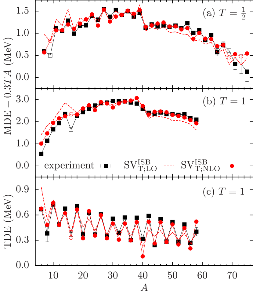
Figure 1: (Color online) MDEs in the $T=\frac{1}{2}$ (a) and $T=1$ (b) mirror nuclei, and TDEs (c) in isospin triplets, calculated using the SV${}^{\rm ISB}_{\rm T;LO}$ (dashed line) and SV${}^{\rm ISB}_{\rm T;NLO}$ (circles) functionals, in comparison with experimental data (squares) [24, 25]. Open symbols denote outliers excluded from the fit, see text.

To find out whether the improvement of the RMSD, Table 1, is not only a result of the increased number of adjustable parameters (from 1 to 3 parameters for each class), we determined the Bayesian Information Criterion (BIC) [32],

$$\mathrm{BIC}=2n\cdot\ln(\mathrm{RMSD/keV})+p\cdot\ln(n),$$ (5)

where $n$ is the number of data points used for fitting and $p$ is the number of adjustable parameters. This formula for calculating BIC is valid under the same assumptions that are commonly made when defining the least-squared fitting approach (independent distribution of the model errors according to the normal distribution and maximization of the log likelihood with respect to the true variance). Then, the difference of BICs between the LO and NLO models reads:

$$\mathrm{BIC_{LO}}-\mathrm{BIC_{NLO}}=2n\cdot\ln\left(\frac{\mathrm{RMSD_{LO}}}{\mathrm{RMSD_{NLO}}}\right)-2\ln(n).$$ (6)

As it turns out, for class III and II this difference equals 53 and 13, respectively, which strongly favours the NLO model, as it is the one with much lower value of BIC [33]. To sum up, by increasing the number of parameters when going from LO to NLO, our approach leads to a more accurate model that describes the physics better, rather than to a model that overfits the data.

We can now address the question of what is the nature of the introduced ISB terms of the functional, namely, whether they model the strong-force-rooted effects, Coulomb correlations beyond mean field, or both. In this Letter, we address this question by performing a systematic study of the Isobaric Multiplet Mass Equation (IMME) [34, 35], $BE(A,T,T_{z})=a+bT_{z}+cT_{z}^{2}$, and by comparing the DFT results with those obtained within the GFMC approach [20, 21].

The quadratic dependence of binding energies on $T_{z}$, which is assumed in IMME, is motivated by the expansion of the two-body Coulomb force into isoscalar, isovector, and isotensor terms [36], which also motivates the following IMME variant ,

$$BE(A,T,I,T_{z}) = a^{(0)}_{A,T,I}-a^{(1)}_{A,T,I}T_{z}+{\textstyle\frac{1}{2}}a^{(2)}_{A,T,I}\{3T_{z}^{2}-T(T+1)\},$$ (7)

where for the IMME coefficients $a^{(n)}_{A,T,I}$ we used the traditional notation that includes the angular-momentum quantum number $I$.

Of course, for triplets ($T=1$), nuclear masses can always be trivially described by a parabolic dependence on $T_{z}$, so then the information carried by the IMME coefficients is exactly the same as that contained in the displacement energies discussed above, with $\mathrm{MDE}=2Ta^{(1)}_{A,T,I}=-2Tb$ and $\mathrm{TDE}=3T^{2}a^{(2)}_{A,T,I}=2T^{2}c$. For higher multiplets ($T>1$), there is an active ongoing debate if higher-order terms, proportional to $T_{z}^{3}$ or $T_{z}^{4}$, are required, see Refs. [37, 38] for brief recent reviews.

We investigate the intrinsic structure of the IMME coefficients by decomposing them into contributions coming from the electromagnetic and contact ISB parts of the functional. We compare the DFT results with those obtained using the GFMC method, split into the electromagnetic and nuclear ISB parts, see Refs. [20, 7, 21]. In this way, we try to bridge the gap between our phenomenological ISB terms with LECs fitted to many-body data and the AV18 [6] ISB forces with LECs adjusted to two-body scattering data. The GFMC calculations involve high-precision potential AV18, which takes into account the ISB effects due to the one-photon and higher-order electromagnetic effects, isovector kinetic energy, and class-II and class-III strong finite-range regularized interactions. On the other hand, our DFT modelling captures all ISB effects (beyond the mean-field Coulomb) either in two (LO) or six (NLO) LECs corresponding to contact class-II and class-III forces.

Table 2: Contributions of the electromagnetic ($V^{\gamma}$), ISB nuclear ($V^{\rm{ISB}}$), and isoscalar ($H^{\rm{T=0}}$) forces to coefficients $a^{(1)}_{A,T,I}$, see Eq. (7), calculated using the GFMC [21] and ISB DFT at LO and NLO. Theoretical uncertainties of the DFT results are related to the uncertainties of the adjusted LECs. All values are in keV.

$a^{{(1)}}_{A,T,I}$	Model	$V^{\gamma}$		$V^{\rm{ISB}}$		$H^{\rm{T=0}}$		Total		EXP
	GFMC	1056	(1)	62	(0)	68	(3)	1184	(4)
$a^{(1)}_{6,1,0}$	SV${}_{\rm{T;LO}}^{\rm{ISB}}$	1278		320		11		1609	(15)	1174
	SV${}_{\rm{T;NLO}}^{\rm{ISB}}$	1277		118		12		1407	(24)
	GFMC	1478	(2)	106	(1)	27	(10)	1611	(10)
$a^{(1)}_{7,\frac{1}{2},\frac{3}{2}}$	SV${}_{\rm{T;LO}}^{\rm{ISB}}$	1539		472		13		2024	(25)	1644
	SV${}_{\rm{T;NLO}}^{\rm{ISB}}$	1537		66		14		1617	(48)
	GFMC	1675	(1)	102	(1)	43	(6)	1813	(6)
$a^{(1)}_{8,1,2}$	SV${}_{\rm{T;LO}}^{\rm{ISB}}$	1730		368		18		2116	(17)	1770
	SV${}_{\rm{T;NLO}}^{\rm{ISB}}$	1726		189		21		1936	(21)
	GFMC	2155	(7)	110	(1)	—		2170	(8)
$a^{(1)}_{10,1,0}$	SV${}_{\rm{T;LO}}^{\rm{ISB}}$	2154		354		25		2533	(16)	2329
	SV${}_{\rm{T;NLO}}^{\rm{ISB}}$	2146		296		31		2474	(13)
	SV${}_{\rm{T;LO}}^{\rm{ISB}}$	2432		505		26		2964	(26)
$a^{(1)}_{11,\frac{1}{2},\frac{3}{2}}$										2764
	SV${}_{\rm{T;NLO}}^{\rm{ISB}}$	2424		260		33		2717	(33)
	SV${}_{\rm{T;LO}}^{\rm{ISB}}$	2589		419		31		3040	(19)
$a^{(1)}_{12,1,1}$										2767
	SV${}_{\rm{T;NLO}}^{\rm{ISB}}$	2584		257		35		2876	(21)
	SV${}_{\rm{T;LO}}^{\rm{ISB}}$	2736		345		39		3120	(21)
$a^{(1)}_{13,\frac{1}{2},\frac{1}{2}}$										3003
	SV${}_{\rm{T;NLO}}^{\rm{ISB}}$	2736		244		38		3018	(33)
	SV${}_{\rm{T;LO}}^{\rm{ISB}}$	3006		489		34		3529	(22)
$a^{(1)}_{14,1,0}$										3276
	SV${}_{\rm{T;NLO}}^{\rm{ISB}}$	3002		185		38		3225	(34)

Table 3: Same as in Table 2 but for coefficients $a^{(2)}_{A,T,I}$.

$a^{{(2)}}_{A,T,I}$	Model	$V^{\gamma}$		$V^{\rm{ISB}}$		$H^{\rm{T=0}}$		Total		EXP
	GFMC	153	(1)	112	(2)	5	(4)	270	(5)
$a^{(2)}_{6,1,0}$	SV${}_{\rm{T;LO}}^{\rm{ISB}}$	171		132		7		309	(17)	223
	SV${}_{\rm{T;NLO}}^{\rm{ISB}}$	165		43		17		225	(16)
	GFMC	136	(1)	$-$3	(2)	10	(5)	139	(5)
$a^{(2)}_{8,1,2}$	SV${}_{\rm{T;LO}}^{\rm{ISB}}$	146		27		8		181	(12)	127
	SV${}_{\rm{T;NLO}}^{\rm{ISB}}$	142		5		15		161	(18)
	GFMC	178	(1)	119	(18)	—		297	(19)
$a^{(2)}_{10,1,0}$	SV${}_{\rm{T;LO}}^{\rm{ISB}}$	156		94		10		260	(13)	242
	SV${}_{\rm{T;NLO}}^{\rm{ISB}}$	146		76		26		248	(9)
$a^{(2)}_{12,1,1}$	SV${}_{\rm{T;LO}}^{\rm{ISB}}$	135		19		7		160	(6)	162
	SV${}_{\rm{T;NLO}}^{\rm{ISB}}$	134		15		12		161	(10)
$a^{(2)}_{14,1,0}$	SV${}_{\rm{T;LO}}^{\rm{ISB}}$	146		68		-4		211	(10)	225
	SV${}_{\rm{T;NLO}}^{\rm{ISB}}$	142		67		-3		207	(7)

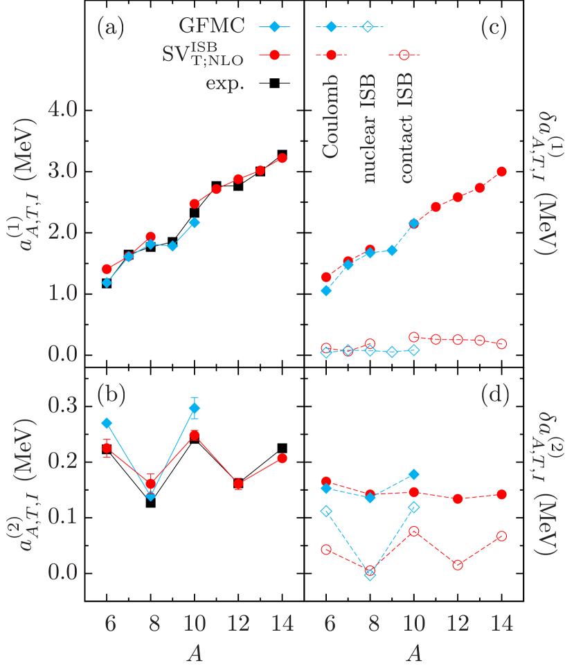
Figure 2: (Color online) IMME coefficients $a^{(1)}_{A,T,I}$ (a) and $a^{(2)}_{A,T,I}$ (b), see Eq. (7), and contributions to the IMME coefficients ${\delta}a^{(1)}_{A,T,I}$ (c) and ${\delta}a^{(2)}_{A,T,I}$ (d) due to electromagnetic (full symbols), nuclear ISB (open diamonds), and contact ISB (open circles) forces. For every $A$, quantum numbers $T$ and $I$ are listed in Tables 2 and 3.

The DFT and GFMC results are collected in Tables 2 and 3 together with experimental data [24, 25]. As shown in the Tables and visualized in Figs. 2(a) and 2(b), the DFT and GFMC results are of a comparable quality. In the two lightest triplets ($A=6$ and 8), coefficients $a^{(1)}_{A,T,I}$ are slightly better described by the GFMC. This approach, unlike the DFT, probably takes better into account the continuum effects that may be present here due the proximity of the proton-emission threshold. Indeed, in ⁶Be (S_p=590keV) and ⁸B (S_p=136keV), relatively large Thomas-Ehrman shifts [39, 40, 41] are seen in the spectra [25].

In the same two lightest triplets, coefficients $a^{(2)}_{A,T,I}$ are better described by the ISB DFT. It should be said, however, that the experimental value of $a^{(2)}_{8,1,2}$ is somewhat uncertain, as it relays on a model-dependent evaluation of the isospin mixing in a near-degenerate doublet of $I=2^{+}$ states at 16.626 and 16.922 MeV in ⁸Be. In this work, following the analysis of Ref. [21], we adopted the value of 16.8 MeV for the excitation energy of the so called empirical $T$=1 state and, consequently, 128 keV for the value of $a^{(2)}_{8,1,2}$. Taking instead the value of 16.724 MeV, which results from a simple two-level mixing model, would lead to $a^{(2)}_{8,1,2}$=0.179 keV.

It is striking that, except for $A$=6, both models predict almost the same contributions to $a^{(1)}_{A,T,I}$ coming from the electromagnetic force, see Fig. 2(c). Since the GFMC approach contains Coulomb correlations beyond mean field and DFT does not, this may hint to the fact that such correlations may not be essential in reproducing the ISB effects in the many-body context.

Except for the $A$=10 triplet, the nuclear ISB contributions in GFMC are also consistent with contact ISB contributions in DFT. Note, however, that in this case the GFMC (DFT) underestimates (overestimates) the $a^{(1)}_{10,1,0}$ coefficient by a similar amount. It is likely, that the differences reflect a too weak (too strong) nuclear (contact) ISB forces in the GFMC (DFT) calculations. This consistency supports the interpretation that the contact ISB DFT terms in fact describes mostly the nuclear ISB effects. Note in addition that at LO, the ISB DFT contributions to the isovector coefficients are almost three times larger than the GFMC values. This underlines the importance of the NLO class-III corrections introduced in this work, which seem to be indispensable for a proper treatment of the ISB effects in the isovector channel.

The NLO ISB DFT terms are equally important for description of the isotensor channel. Indeed, the isotensor coefficients $a^{(2)}_{A,T,I}$ are exceptionally well reproduced at NLO, even better than in the GFMC calculations, see Fig. 2(b). The individual contributions due to electromagnetic and nuclear/contact in GFMC/DFT ISB effects, see Fig. 2(d), are comparable in both models.

In the DFT calculations, the staggering in $a^{(2)}_{A,T,I}$, Fig. 2(d), comes entirely from the contact class-II force. The details depend, however, on the order of approximation. At LO (NLO), the staggering is due to the class-II time-odd (time-even) mean fields, see Figs. 3. In the GFMC calculations, both the electromagnetic and strong class-II forces contribute to the staggering, but the latter contribution prevails. We also note here that in the nuclear shell model, the staggering is explained in terms of the $J=0$ neutron-proton pairing, see Ref. [13].

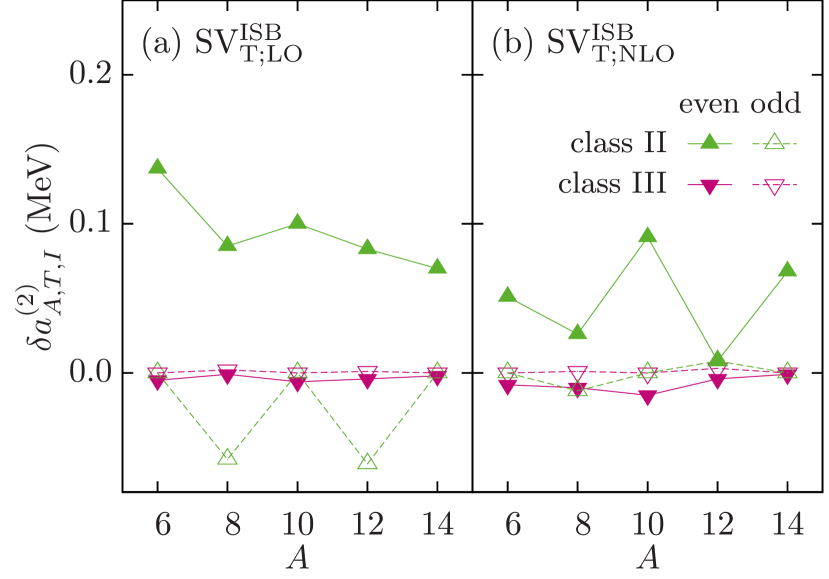
Figure 3: (Color online) Contributions to the ISB DFT IMME coefficients ${\delta}a^{(2)}_{A,T,I}$ due to time-even (full symbols) and time-odd (open symbols) class-II (up triangles) and class-III (down triangles) mean fields, determined at LO (a) and NLO (b).

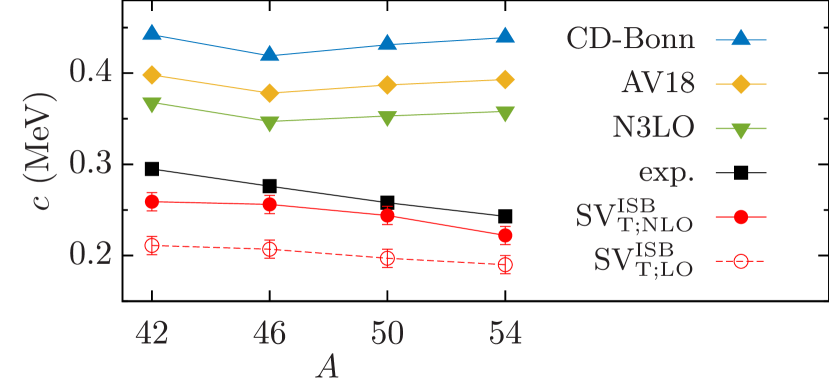
Figure 4: (Color online) Isotensor coefficients $c$ calculated within the ISB DFT and shell-model-based ab initio approach at 3^rd order [10].

Recently, Ormand et al. [10] performed shell-model-based ab initio study of the isotensor IMME coefficients $c$ in the $pf$-shell isospin triplets ($A=42$, 46, 50, and 54). Their results systematically overestimate the experimental values, irrespective of which high-precision potential, CD-Bonn [3], AV18 [6], or N3LO [9], was used in the calculations, see Fig. 4. Conversely, our ISB DFT calculations at LO and NLO systematically underestimate the experimental data, but at NLO the level of agreement greatly improves. The DFT and shell-model-based ab initio methods predict very different contributions to $c$ due to the Coulomb and contact/nuclear ISB forces. At present it is impossible, however, to draw deeper conclusions, because the results of Ref. [10] do not seem yet to converge with respect to the order of calculation, and because those for the $A=4n$ triplets are not yet available. The DFT results presented in this Letter may thus serve as a baseline for future comparisons of both approaches in heavy nuclei.

The ISB character of the strong interaction manifests itself not only in the values of MDE and TDE. One can expect it to be important in describing $\beta$ decays, differences of energies of levels of nuclei in isospin multiplets (mirror and triplet energy differences, MED and TED), giant and Gamow-Teller resonances, etc. The ISB DFT seems to be a perfect tool to study all these observables. Currently our group is working on the effects of the short-range ISB terms of class III on the $\beta$ decays in mirror nuclei and on MEDs in rotational bands. The results will be published in forthcoming publications.

In summary, we performed systematic study of mirror and triplet displacement energies, or equivalently, isovector and isotensor IMME coefficients, using the extended DFT approach that includes proton-neutron mixing and contact ISB terms at LO and NLO. In light nuclei, we compared the obtained IMME coefficients with the results of existing GFMC calculations. We focused on comparing partial contributions due to electromagnetic and nuclear ISB terms.

We showed that the NLO terms greatly improve the agreement of the DFT results with data, and that the DFT and GFMC calculations reproduce empirical IMME coefficients comparably well. But most importantly, we showed that the Coulomb contributions to the IMME coefficients are similar in both approaches, which implies that the Coulomb correlations beyond mean field may not be crucial in reproducing the ISB effects in the many-body context.

We thank the authors of Ref. [10] for sending us numerical values of their results. This work was supported in part by the Polish National Science Centre under Contract Nos. 2014/15/N/ST2/03454 and 2015/17/N/ST2/04025, by the Academy of Finland and University of Jyväskylä within the FIDIPRO program, and by the STFC Grants No. ST/M006433/1 and No. ST/P003885/1. We acknowledge the CSC-IT Center for Science Ltd., Finland, and CIŚ Świerk Computing Center, Poland, for the allocation of computational resources.

References

- [1] Heisenberg W 1932 Zeitschrift für Physik 77 1–11 URL https://doi.org/10.1007/BF01342433
- [2] Wigner E 1937 Phys. Rev. 51(2) 106 URL http://link.aps.org/doi/10.1103/PhysRev.51.106
-
[3]
Machleidt R 2001 Phys. Rev. C 63 024001
URL
https://link.aps.org/doi/10.1103/PhysRevC.63.024001 - [4] Henley E M and Miller G A 1979 Mesons in Nuclei (North Holland)
- [5] Miller G A and van Oers W H T 1995 Symmetries and Fundamental Interactions in Nuclei (World Scientific)
- [6] Wiringa R B, Stoks V G J and Schiavilla R 1995 Phys. Rev. C 51(1) 38–51 URL https://link.aps.org/doi/10.1103/PhysRevC.51.38
- [7] Wiringa R B, Pastore S, Pieper S C and Miller G A 2013 Phys. Rev. C 88(4) 044333 URL http://link.aps.org/doi/10.1103/PhysRevC.88.044333
- [8] Walzl M, Meißner U G and Epelbaum E 2001 Nuclear Physics A 693 663 – 692 ISSN 0375-9474 URL http://www.sciencedirect.com/science/article/pii/S0375947401009691
- [9] Epelbaum E, Hammer H W and Meißner U G 2009 Rev. Mod. Phys. 81(4) 1773–1825 URL https://link.aps.org/doi/10.1103/RevModPhys.81.1773
- [10] Ormand W E, Brown B A and Hjorth-Jensen M 2017 Phys. Rev. C 96(2) 024323 URL https://link.aps.org/doi/10.1103/PhysRevC.96.024323
- [11] Satuła W, Dobaczewski J, Nazarewicz W and Rafalski M 2009 Phys. Rev. Lett. 103(1) 012502 URL http://link.aps.org/doi/10.1103/PhysRevLett.103.012502
- [12] Ormand W and Brown B 1989 Nucl. Phys. A 491 1 ISSN 0375-9474 URL http://www.sciencedirect.com/science/article/pii/0375947489902030
- [13] Zuker A P, Lenzi S M, Martinez-Pinedo G and Poves A 2002 Phys. Rev. Lett. 89(14) 142502 URL https://link.aps.org/doi/10.1103/PhysRevLett.89.142502
- [14] Kaneko K, Sun Y, Mizusaki T, Tazaki S and Ghorui S 2017 Physics Letters B 773 521 – 526 ISSN 0370-2693 URL http://www.sciencedirect.com/science/article/pii/S0370269317306780
- [15] Suzuki T, Sagawa H and Van Giai N 1993 Phys. Rev. C 47(4) R1360–R1363 URL http://link.aps.org/doi/10.1103/PhysRevC.47.R1360
- [16] Brown B A, Richter W A and Lindsay R 2000 Physics Letters B 483 49 – 54 ISSN 0370-2693 URL http://www.sciencedirect.com/science/article/pii/S037026930000589X
- [17] Bączyk P, Dobaczewski J, Konieczka M, Satuła W, Nakatsukasa T and Sato K 2018 Physics Letters B 778 178 – 183 URL https://arxiv.org/abs/1701.04628v3
- [18] Sato K, Dobaczewski J, Nakatsukasa T and Satuła W 2013 Phys. Rev. C 88(6) 061301 URL https://link.aps.org/doi/10.1103/PhysRevC.88.061301
- [19] Sheikh J A, Hinohara N, Dobaczewski J, Nakatsukasa T, Nazarewicz W and Sato K 2014 Phys. Rev. C 89(5) 054317 URL http://link.aps.org/doi/10.1103/PhysRevC.89.054317
- [20] Wiringa R B, Pieper S C, Carlson J and Pandharipande V R 2000 Phys. Rev. C 62(1) 014001 URL https://link.aps.org/doi/10.1103/PhysRevC.62.014001
- [21] Carlson J, Gandolfi S, Pederiva F, Pieper S C, Schiavilla R, Schmidt K E and Wiringa R B 2015 Rev. Mod. Phys. 87(3) 1067–1118 URL http://link.aps.org/doi/10.1103/RevModPhys.87.1067
- [22] Schunck N, Dobaczewski J, Satuła W, Bączyk P, Dudek J, Gao Y, Konieczka M, Sato K, Shi Y, Wang X and Werner T 2017 Computer Physics Communications 216 145 – 174 ISSN 0010-4655 URL http://www.sciencedirect.com/science/article/pii/S0010465517300942
- [23] Dobaczewski J et al., to be published
- [24] Wang M, Audi G, Kondev F, Huang W, Naimi S and Xu X 2017 Chinese Physics C 41 030003 URL http://stacks.iop.org/1674-1137/41/i=3/a=030003
- [25] Evaluated Nuclear Structure Data File, http://www.nndc.bnl.gov/ensdf/ URL http://www.nndc.bnl.gov/ensdf/
- [26] Zhang Y H, Zhang P, Zhou X H, Wang M, Litvinov Y A, Xu H S, Xu X, Shuai P, Lam Y H, Chen R J, Yan X L, Bao T, Chen X C, Chen H, Fu C Y, He J J, Kubono S, Liu D W, Mao R S, Ma X W, Sun M Z, Tu X L, Xing Y M, Zeng Q, Zhou X, Zhan W L, Litvinov S, Blaum K, Audi G, Uesaka T, Yamaguchi Y, Yamaguchi T, Ozawa A, Sun B H, Sun Y and Xu F R 2018 Phys. Rev. C 98(1) 014319 URL https://link.aps.org/doi/10.1103/PhysRevC.98.014319
- [27] Dobaczewski J, Nazarewicz W and Reinhard P G 2014 Journal of Physics G: Nuclear and Particle Physics 41 074001 URL http://stacks.iop.org/0954-3899/41/i=7/a=074001
- [28] Beiner M, Flocard H, Giai N V and Quentin P 1975 Nuclear Physics A 238 29 – 69 ISSN 0375-9474 URL http://www.sciencedirect.com/science/article/pii/0375947475903383
- [29] Satuła W and Dobaczewski J 2014 Phys. Rev. C 90(5) 054303 URL https://link.aps.org/doi/10.1103/PhysRevC.90.054303
- [30] Tarpanov D, Toivanen J, Dobaczewski J and Carlsson B G 2014 Phys. Rev. C 89(1) 014307 URL http://link.aps.org/doi/10.1103/PhysRevC.89.014307
- [31] Lepage G 1997 nucl-th/9706029 URL https://arxiv.org/abs/nucl-th/9706029
- [32] Priestley M B 1981 Spectral Analysis and Time Series (Academic Press) p 375
- [33] Kass R E and Raftery A E 1995 Journal of the American Statistical Association 90 773–795 URL https://www.tandfonline.com/doi/abs/10.1080/01621459.1995.10476572
- [34] Wigner E P 1958 Proceedings of the Robert A. Welsch Conference on Chemical Research, Vol. 1 ed Milligan W D (R. A. Welsch Foundation, Houston, TX) p 88
- [35] Weinberg S and Treiman S B 1959 Phys. Rev. 116(2) 465–468 URL https://link.aps.org/doi/10.1103/PhysRev.116.465
-
[36]
Peshkin M 1961 Phys. Rev. 121(2) 636
URL
http://link.aps.org/doi/10.1103/PhysRev.121.636 - [37] Nesterenko D A, Kankainen A, Canete L, Block M, Cox D, Eronen T, Fahlander C, Forsberg U, Gerl J, Golubev P, Hakala J, Jokinen A, Kolhinen V S, Koponen J, Lalović N, Lorenz C, Moore I D, Papadakis P, Reinikainen J, Rinta-Antila S, Rudolph D, Sarmiento L G, Voss A and Äystö J 2017 Journal of Physics G: Nuclear and Particle Physics 44 065103 URL http://stacks.iop.org/0954-3899/44/i=6/a=065103
- [38] Brodeur M, Kwiatkowski A A, Drozdowski O M, Andreoiu C, Burdette D, Chaudhuri A, Chowdhury U, Gallant A T, Grossheim A, Gwinner G, Heggen H, Holt J D, Klawitter R, Lassen J, Leach K G, Lennarz A, Nicoloff C, Raeder S, Schultz B E, Stroberg S R, Teigelhöfer A, Thompson R, Wieser M and Dilling J 2017 Phys. Rev. C 96(3) 034316 URL https://link.aps.org/doi/10.1103/PhysRevC.96.034316
-
[39]
Thomas R G 1951 Phys. Rev. 81 148
URL
https://link.aps.org/doi/10.1103/PhysRev.81.148 - [40] Ehrman J B 1951 Phys. Rev. 81 412 URL http://link.aps.org/doi/10.1103/PhysRev.81.412
-
[41]
Thomas R G 1952 Phys. Rev. 88 1109
URL
http://link.aps.org/doi/10.1103/PhysRev.88.1109