From classical to quantum models: the regularising rôle of integrals, symmetry and probabilities

Abstract.

In physics, one is often misled in thinking that the mathematical model of a system is part of or is that system itself. Think of expressions commonly used in physics like “point” particle, motion “on the line”, “smooth” observables, wave function, and even “going to infinity”, without forgetting perplexing phrases like “classical world” versus “quantum world”…. On the other hand, when a mathematical model becomes really inoperative in regard with correct predictions, one is forced to replace it with a new one. It is precisely what happened with the emergence of quantum physics. Classical models were (progressively) superseded by quantum ones through quantization prescriptions. These procedures appear often as ad hoc recipes. In the present paper, well defined quantizations, based on integral calculus and Weyl-Heisenberg symmetry, are described in simple terms through one of the most basic examples of mechanics. Starting from (quasi-) probability distribution(s) on the Euclidean plane viewed as the phase space for the motion of a point particle on the line, i.e., its classical model, we will show how to build corresponding quantum model(s) and associated probabilities (e.g. Husimi) or quasi-probabilities (e.g. Wigner) distributions. We highlight the regularizing rôle of such procedures with the familiar example of the motion of a particle with a variable mass and submitted to a step potential.

1. Introduction

A world of mathematical models for one “thing” in the “World”

The physical laws are expressed in terms of combinations of mathematical symbols, numbers, functions, geometries, relations … These combinations take place within a mathematical model for the system, a part of the so-called objective reality under consideration. Such a language and related concepts are in constant development since the set of phenomenons which are accessible to our scientific understanding is constantly broadening, or at least, reshaped. Now, a model for a system is usually scale dependent. It depends on a ratio of physical, i.e., measurable, quantities, like amounts of substance, lengths, time(s), sizes, impulsions, actions, energies … In certain cases, a radical change of scale, radical in the mathematical sense of limit, for a model amounts to “quantize” or “de-quantize”. As a matter of fact, one decides on the validity of a classical model versus a quantum one for a given physical system if the action(s) which is (are) characteristics of the latter, e.g. $\sqrt[3]{\mbox{{spatial size}}}\times$momentum or energy$\times$time duration or angular momentum, is (are) $\gg\hbar$. One changes perspective, one can say that our understanding changes its (mathematical) glasses!

Exactness of models and probabilities

Nothing is mathematically exact from the physical point of view. A mathematical model in Physics is never for ever. Its suitability is time dependent because it is scale dependent. In order to be adjusted to experimental observations and predictions, it has to be modified more or less radically, even radically changed. In the relation modeler $\leftrightarrow$ modelled object, there is probability, $\sim$ degree of epistemic confidence in the suitability of the model. Hence emerges the necessity of some coarse-graining of the initial mathematical model supposed to describe a certain ontic entity or fact.

For instance, irrational numbers are far beyond human perception but physical laws are usually (since a few centuries) expressed in terms of real numbers, $\mathbb{R}$, built from limit notions (limit of Cauchy sequences of rational numbers). Now, an infinite amount of energy would be needed to measure the location of one point on the real line! A coarse-graining, or quantization in the sense of signal analysis, is naturally requested on an operational level.

Even the notion of contextuality, which describes how or whether the details of an observation affect what is observed, cannot be dissociated from the mathematical model used for the definition of the object, its observation, and its interpretation.

The aim of this paper is to show that the construction of a quantum model from a classical one pertains, in a certain sense, to that type of coarse-graining procedure. The procedure is illustrated with one of the most elementary examples in mechanics, namely the motion of a point particle on the straight $\sim$ real line $\sim$ $\mathbb{R}$ , for which the phase space is the plane shown in Figure 1.

(1.1) $$\mathbb{R}^{2}=\{\boldsymbol{r}=(q,p)\,,\,q,p\in\mathbb{R}\}\,.$$

We then establish the quantum versions of this classical model by developing an approach combining probability (the coarse-graining) with symmetry and integral calculus.

A part of this work will certainly appear familiar to most of the readership. However we have chosen to present the material, e.g., Weyl-Heisenberg and Galilean symmetries, basic rules of quantum formalism, in a somewhat uncommon and self-contained way, and we want to emphasize the benchmark role played by obvious symmetry requirement(s) in any quantization procedure.

Figure 1. Set of initial conditions $\sim$ phase space for the motion of a point particle on the real line.

In Section 2 are recalled the essential features of the quantum formalism and the way it is established from Hamiltonian classical mechanics. A survey of various quantization methods is also sketched. The covariant Weyl-Heisenberg integral quantization is the subject of Section 3. Starting from the translation symmetry of the Euclidean plane, we show how to reach its non commutative representation underlying the corresponding quantum model of the phase space through integral maps involving operator-valued measures. In Section 4 the above procedure is implemented in the case of elementary functions on the phase space, namely coordinates, quadratic expressions, functions of $q$ (resp. $p$) only. We point out the similarities and differences between their respective quantum versions in function of the operator-valued measure underlying a specific integral quantization. We show in Section 5 that the method easily applies to Hamiltonian expressions constrained by the so-called shadow Galilean invariance, an important notion that we explain in detail because it fully justifies the concept of variable mass. We give in Section 6 a few examples of these operator-valued measures, and discuss about their relevance in dealing with specific classical functions. Section 7 is devoted to the description of the probabilistic aspects of our quantization procedure and its reversal under the form of quantum phase space portraits. This leads to an interesting analogy with the intensity of a diffraction pattern resulting from the coarse graining of the idealistic phase space $\mathbb{R}^{2}$. The general method is illustrated in Section 8 with the textbook model of a variable mass particle whose one-dimensional motion is constrained by a potential barrier. We conclude in Section 9 by giving some insight about the generalisation of the approach to phase spaces presenting different symmetries, and to manifolds embedded in higher dimensional phase spaces.

2. Considerations on standard and other quantizations

The basic, or so-called canonical, quantization procedure starts from the phase space $\mathbb{R}^{2}$,

(2.1) $$\mathbb{R}^{2}\ni(q,p) \mapsto\ \mbox{self-adjoint}\ (Q,P)\,,\quad[Q,P]=\mathsf{i}\hbar I\,,$$

(2.2) $$f(q,p) \mapsto f(Q,P)\mapsto(\mathrm{Sym}f)(Q,P)\,,$$

where $\mathrm{Sym}$ stands for a certain choice of symmetrisation of the operator-valued function. We remind that $[Q,P]=\mathsf{i}\hbar I$ holds true with (essentially) self-adjoint $Q$, $P$, only if both have continuous spectrum $(-\infty,+\infty)$. We also remind that a quantum observable is an essentially ($\sim$ no ambiguity) self-adjoint operator in the Hilbert space $\mathcal{H}$ of quantum states, since the key for (sharp) quantum measurement is encapsulated in the spectral theorem for a bounded or unbounded self-adjoint operator $A$. The latter asserts that $A$ has a real spectrum with integral representation

(2.3) $$A=\int_{\Sigma\subset\mathbb{R}}\lambda\,\mathrm{d}E_{A}(\lambda)\,,$$

involving a normalised projective-operator measure $\mathrm{d}E_{A}(\lambda):=E_{A}((\lambda,\lambda+\mathrm{d}\lambda))$. The expression projective means that

(2.4) $$E_{A}(\Sigma\cap\Sigma^{\prime})=E_{A}(\Sigma)\,E_{A}(\Sigma^{\prime})$$

whereas normalisation means resolution of the identity in $\mathcal{H}$,

(2.5) $$\int_{\Sigma\subset\mathbb{R}}\mathrm{d}E_{A}(\lambda)=I\,.$$

In this context, the position operator is self-adjoint with spectrum $\mathbb{R}$

(2.6) $$Q=\int_{\mathbb{R}}\lambda\,|\lambda\rangle\langle\lambda|\,\mathrm{d}\lambda\,,\qquad\langle x|\lambda\rangle=\delta(x-\lambda)\,.$$

and the Hilbert space of quantum states is realized as functions $\psi(x)$, the wave functions, which are square integrable on the spectrum of the position operator $Q$. At the heart of the concept of localisability, the variable $x$ has to be interpreted as a (measurable) element of the spectrum of $Q$: it is an essential part of the quantum model, and not of the classical one. Moreover, its definition is not ambiguous in Galilean quantum mechanics [1, 2]. Accordingly, the action of $P$ on this Hilbert space results from $[Q,P]=\mathsf{i}\hbar I$

(2.7) $$P\psi(x)=-\mathsf{i}\hbar\frac{\mathrm{d}}{\mathrm{d}x}\psi(x)\,.$$

This simple scheme presented in many introductive textbooks to quantum mechanics immediately raises fundamental questions like what about singular $f$, e.g. the angle or phase $\arctan(p/q)$? What about other phase space geometries? Barriers or other impassable boundaries? The motion on a circle (the question of quantum angle and localisation on the circle)? In a bounded interval? On the positive half-line (singularity at the origin)? …. Despite their elementary aspects, these disturbing examples leave open many questions both on mathematical and physical levels, irrespective of the manifold of quantization procedures, like Lagrangian & Path Integral Quantization (Dirac 1932, Feynman, thesis, 1942). Or, after approaches by Weyl (1927), Groenewold (1946), Moyal (1947), Geometric Quantization, Kirillov (1961) Souriau (1966), Kostant (1970), Deformation Quantization, Bayen, Flato, Fronsdal, Lichnerowicz, Sternheimer (1978), Fedosov (1985), Kontsevich (2003), coherent state or anti-Wick or Toeplitz quantization with Klauder (1961), Berezin (1974) and others…, see for instance illuminating articles like [3], comprehensive reviews like [4] [5], and more recent volumes like [6] [7], about these various approaches. Indeed, most of these methods, despite their beautiful mathematical content, are often too demanding for some classical models to be consistently quantized.

On the other hand, it is fair to acknowledge that canonical quantization is quasi-universally accepted in view of its numerous experimental validations, one of the most famous and simplest one going back to the early period of quantum mechanics with the quantitative prediction (1925) of the isotopic effect in vibrational spectra of diatomic molecules (see [8] and references therein). These data validated the canonical quantization, contrary to the Bohr-Sommerfeld ansatz (which predicts no isotopic effect). Nevertheless this does not prove that another method of quantization fails to yield the same prediction. Moreover the canonical quantization appears as too rigid or even untractable in some circumstances, as was underlined above. As a matter of fact, the canonical or the Weyl-Wigner integral quantization maps $f(q)$ to $f(Q)$ (resp. $f(p)$ to $f(P)$), and so might be unable to cure or regularise a given classical singularity, particularly with regard to the requirement of essential self-adjointness for basic operators, which is not guaranteed anymore. This marks one more difference between classical and quantum models. In Physics one works mostly (if not always!) with effective models, and an effective quantum model is expected, for practical reasons, to be more regular than its classical one. The latter is often viewed as too mathematically idealised.

3. Covariant integral quantization of the motion on the line

In this section, we describe our approach to the quantization of the motion on the line. Precisely, we transform a function $f(q,p)\equiv f(\boldsymbol{r})$ into an operator $A_{f}$ in some Hilbert space $\mathcal{H}$ through a linear map which sends the function $f=1$ to the identity operator in $\mathcal{H}$ and which respects the basic translational symmetry of the phase space. The trick is to use ressources of measure/integral calculus, where we can ignore points or lines to some extent. A probabilistic content will be one of the most appealing outcomes of the procedure.

3.1. The quantization map

We define the integral quantization of the motion on the line as the linear map

(3.1) $$f(\boldsymbol{r})\mapsto A_{f}=\int_{\mathbb{R}^{2}}f(\boldsymbol{r})\,\mathfrak{Q}(\boldsymbol{r})\,\frac{\mathrm{d}^{2}\boldsymbol{r}}{2\pi c_{\mathfrak{Q}}}\,,\quad\mathrm{d}^{2}\boldsymbol{r}=\mathrm{d}q\,\mathrm{d}p\,.$$

where $c_{\mathfrak{Q}}$ is a positive constant, whose meaning will be given later, and $\mathfrak{Q}(\boldsymbol{r})/(2\pi c_{\mathfrak{Q}})$ is a family of operators which solve the identity in $\mathcal{H}$ with respect to the Lebesgue measure $\mathrm{d}^{2}\boldsymbol{r}$,

(3.2) $$\int_{\mathbb{R}^{2}}\mathfrak{Q}(\boldsymbol{r})\,\frac{\mathrm{d}^{2}\boldsymbol{r}}{2\pi c_{\mathfrak{Q}}}=I\,.$$

Hence the identity $I$ is the quantized version of the function $f=1$. It is clear that we can ignore the immediate solution $\mathfrak{Q}(\boldsymbol{r})=w(\boldsymbol{r})I$ with

$$\int_{\mathbb{R}^{2}}w(\boldsymbol{r})\,\dfrac{\mathrm{d}^{2}\boldsymbol{r}}{2\pi c_{\mathfrak{Q}}}=1\,,$$

which leads to the trivial quantization

$$A_{f}=\langle f\rangle_{w}\,I\quad\mbox{with}\quad\langle f\rangle_{w}:=\int_{\mathbb{R}^{2}}f(\boldsymbol{r})\,w(\boldsymbol{r})\,\frac{\mathrm{d}^{2}\boldsymbol{r}}{2\pi c_{\mathfrak{Q}}}\,,$$

i.e., to the classical statistical mechanics where $w(\boldsymbol{r})$ is chosen as a distribution function with respect to the measure $\mathrm{d}^{2}\boldsymbol{r}/(2\pi c_{\mathfrak{Q}})$.

In addition to (3.2), we impose the family $\mathfrak{Q}(\boldsymbol{r})$ to obey a symmetry condition issued from the homogeneity of the phase space. Indeed, the choice of the origin in $\mathbb{R}^{2}$ is arbitrary. Hence we must have translational covariance in the sense that the quantization of the translated of $f$ is unitarily equivalent to the quantization of $f$

(3.3) $$U(\boldsymbol{r}_{0})\,A_{f}\,U(\boldsymbol{r}_{0})^{{\dagger}}=A_{\mathcal{T}(\boldsymbol{r}_{0})f}\,,\quad\left(\mathcal{T}(\boldsymbol{r}_{0})f\right)(\boldsymbol{r}):=f\left(\boldsymbol{r}-\boldsymbol{r}_{0}\right)$$

So $\boldsymbol{r}\mapsto U(\boldsymbol{r})$ has to be a unitary, possibly projective, representation of the abelian group $\mathbb{R}^{2}$ Then, from (3.3) and the translational invariance of $\mathrm{d}^{2}\boldsymbol{r}=\mathrm{d}q\,\mathrm{d}p$, the operator valued function $\mathfrak{Q}(\boldsymbol{r})$ has to obey

(3.4) $$U(\boldsymbol{r}_{0})\,\mathfrak{Q}(\boldsymbol{r})\,U^{{\dagger}}(\boldsymbol{r}_{0})=\mathfrak{Q}\left(\boldsymbol{r}+\boldsymbol{r}_{0}\right)$$

A solution to (3.4) is found by picking an operator $\mathfrak{Q}_{0}\equiv\mathfrak{Q}(\boldsymbol{0})$ and write

(3.5) $$\mathfrak{Q}\left(\boldsymbol{r}\right):=U(\boldsymbol{r})\,\mathfrak{Q}_{0}\,U^{{\dagger}}(\boldsymbol{r})$$

Then the resolution of the identity holds from Schur’s Lemma [9] if $U$ is irreducible, and if the operator-valued integral (3.2) makes sense, i.e., if the choice of the fixed operator $\mathfrak{Q}_{0}$ is valid.

3.2. Toward projective unitary irreducible representations of $\mathbb{R}^{2}$

Any unitary representation $\boldsymbol{r}\mapsto U(\boldsymbol{r})$ of the abelian group $\mathbb{R}^{2}$ has the following properties

(3.6) $$U(\boldsymbol{0})=I\,,\quad U^{{\dagger}}(\boldsymbol{r})=U(-\boldsymbol{r})\,,\quad U(\boldsymbol{r})\,U(\boldsymbol{r}^{\prime})=U(\boldsymbol{r}+\boldsymbol{r}^{\prime})\,.$$

Therefore, any true unitary irreducible representation of $\mathbb{R}^{2}$ is one-dimensional (Fourier!):

(3.7) $$\boldsymbol{r}\mapsto U_{\boldsymbol{k}}(\boldsymbol{r})=e^{\mathsf{i}\boldsymbol{k}\cdot\boldsymbol{r}}=e^{\mathsf{i}(k_{1}q+k_{2}p)}\,.$$

Now, if we pick one of these representations, then the integral quantization that it defines from (3.5) is barred due to absence of resolution of the identity,

(3.8) $$\mathfrak{Q}(\boldsymbol{r})=\mathfrak{Q}_{0}\,,\quad\Rightarrow\quad\int_{\mathbb{R}^{2}}\mathfrak{Q}(\boldsymbol{r})\,\frac{\mathrm{d}^{2}\boldsymbol{r}}{2\pi}=\infty\,.$$

The alternative is to deal with projective unitary representation of $\mathbb{R}^{2}$ of the form

(3.9) $$U(\boldsymbol{0}) =I\,,\quad U^{{\dagger}}(\boldsymbol{r})=U(-\boldsymbol{r})\,,$$

(3.10) $$U(\boldsymbol{r})\,U(\boldsymbol{r}^{\prime}) =e^{\mathsf{i}\xi(\boldsymbol{r},\boldsymbol{r}^{\prime})}U(\boldsymbol{r}+\boldsymbol{r}^{\prime})$$

where the real valued $\xi$ is accountable for the non commutativity of the representation, a central feature of the family of the $A_{f}$’s,

(3.11) $$\xi(\boldsymbol{r},\boldsymbol{r}^{\prime})\neq\xi(\boldsymbol{r}^{\prime},\boldsymbol{r})\,.$$

This function has to fulfil cocycle conditions which agree with the group structure of $\mathbb{R}^{2}$ defined by the relations

(3.12) $$U(\boldsymbol{0}) =I\,,\quad U^{{\dagger}}(\boldsymbol{r})=U(-\boldsymbol{r})\,,$$

(3.13) $$U(\boldsymbol{r})\,U(\boldsymbol{r}^{\prime}) =e^{\mathsf{i}\xi(\boldsymbol{r},\boldsymbol{r}^{\prime})}U(\boldsymbol{r}+\boldsymbol{r}^{\prime})\,,$$

and which determine the function $\xi$. We deduce from neutral element and inverse in (3.12)

(3.14) $$\xi(\boldsymbol{r},\boldsymbol{0})=0=\xi(\boldsymbol{0},\boldsymbol{r})\,,\quad\xi(\boldsymbol{r},-\boldsymbol{r})=0=\xi(-\boldsymbol{r},\boldsymbol{r})\,.$$

From associativity $U(\boldsymbol{r})\,(U(\boldsymbol{r}^{\prime})\,U(\boldsymbol{r}^{\prime\prime}))=(U(\boldsymbol{r})\,U(\boldsymbol{r}^{\prime}))U(\boldsymbol{r}^{\prime\prime})$ we have

(3.15) $$\xi(\boldsymbol{r},\boldsymbol{r}^{\prime})+\xi(\boldsymbol{r}+\boldsymbol{r}^{\prime},\boldsymbol{r}^{\prime\prime})=\xi(\boldsymbol{r},\boldsymbol{r}^{\prime}+\boldsymbol{r}^{\prime\prime})+\xi(\boldsymbol{r}^{\prime},\boldsymbol{r}^{\prime\prime})\,.$$

From the Lie group structure of $\mathbb{R}^{2}$, the function $\xi$ has to be smooth. Let us apply $\left.\nabla_{\boldsymbol{r}^{\prime\prime}}\right|_{\boldsymbol{r}^{\prime\prime}=\boldsymbol{0}}$ to (3.15), and define $\nabla_{\boldsymbol{b}}\xi(\boldsymbol{a},\boldsymbol{b}):=\boldsymbol{F}(\boldsymbol{a},\boldsymbol{b})$. We then obtain the functional equation for $\boldsymbol{F}$:

(3.16) $$\boldsymbol{F}(\boldsymbol{r},\boldsymbol{r}^{\prime})=\boldsymbol{F}(\boldsymbol{r}+\boldsymbol{r}^{\prime},\boldsymbol{0})-\boldsymbol{F}(\boldsymbol{r}^{\prime},\boldsymbol{0})\,,$$

whose solution is the linear $\boldsymbol{F}(\boldsymbol{r},\boldsymbol{r}^{\prime})=k\boldsymbol{r},$ for some constant $k$. It follows that $\xi(\boldsymbol{r},\boldsymbol{r}^{\prime})$ is bilinear in $(\boldsymbol{r},\boldsymbol{r}^{\prime})$. From $\xi(\boldsymbol{r},-\boldsymbol{r})=-\xi(\boldsymbol{r},\boldsymbol{r})=0$, the only possibility is that $\xi(\boldsymbol{r},\boldsymbol{r}^{\prime})$ is the symplectic form

(3.17) $$\xi(\boldsymbol{r},\boldsymbol{r}^{\prime})=k\,(qp^{\prime}-q^{\prime}p)\equiv k\,\boldsymbol{r}\wedge\boldsymbol{r}^{\prime}\,.$$

Keeping physical dimensions, the constant $k$ should read $k=1/\ell\wp\neq 0$, where $\ell$ (resp. $\wp$) is some characteristic length (resp. momentum) appropriate to the scale of the model. Thinking of quantum systems, we naturally introduce the Planck constant $\hbar$ such that $\ell\wp=\hbar$.

3.3. From $\mathbb{R}^{2}$ to the Weyl-Heisenberg group and its UIR

Because of the non triviality of $\xi$, we have now to deal with the Weyl-Heisenberg (WH) group,

(3.18) $$\mathrm{WH}=\{(s,\boldsymbol{r})\,,\,s\in\mathbb{R}\,,\,\boldsymbol{r}\in\mathbb{R}^{2}\}\,,\quad(s,\boldsymbol{r})(s^{\prime},\boldsymbol{r}^{\prime})=\left(s+s^{\prime}+\frac{1}{2}\xi(\boldsymbol{r},\boldsymbol{r}^{\prime}),\boldsymbol{r}+\boldsymbol{r}^{\prime}\right)\,,$$

instead of just $\mathbb{R}^{2}$. From von Neumann [10, 11, 6], WH has a unique non trivial UIR, up to equivalence corresponding precisely to the arbitrariness in the choice of $k$:

(3.19) $$(s,\boldsymbol{r})\mapsto\mathcal{U}(s,\boldsymbol{r})=e^{\mathsf{i}s}\,U(\boldsymbol{r})=e^{\mathsf{i}s}\,e^{\mathsf{i}(pQ-qP)/k}$$

where $Q$ and $P$ are the two above-mentionned self-adjoint operators in $\mathcal{H}$ such that $[Q,P]=\mathsf{i}\,\hbar I$. In the present context, $U(\boldsymbol{r})$ is named displacement operator. In the sequel we fix $k=1=\hbar$ for convenience, so that $U(\boldsymbol{r})=e^{\mathsf{i}(pQ-qP)}$ .

3.4. WH covariant integral quantization(s)

From Schur’s Lemma applied to the WH UIR $\mathcal{U}$, or equivalently to $U$ since $e^{\mathsf{i}s}$ is just a phase factor, we confirm the resolution of the identity

(3.20) $$\int_{\mathbb{R}^{2}}\mathfrak{Q}(\boldsymbol{r})\,\frac{\mathrm{d}^{2}\boldsymbol{r}}{2\pi c_{\mathfrak{Q}_{0}}}=I\,,\quad\mathfrak{Q}(\boldsymbol{r})=U(\boldsymbol{r})\mathfrak{Q}_{0}U^{{\dagger}}(\boldsymbol{r})\,,$$

where $\mathfrak{Q}_{0}$ is the fixed operator introduced in (3.5), whose choice is left to us, and which is such that $0<c_{\mathfrak{Q}_{0}}<\infty$. Let us prove that this is possible if $\mathfrak{Q}_{0}$ is trace class, i.e., $\mathrm{Tr}(\mathfrak{Q}_{0})$ is finite. Indeed, let us introduce the function

(3.21) $$\Pi(\boldsymbol{r})=\mathrm{Tr}\left(U(-\boldsymbol{r})\mathfrak{Q}_{0}\right)\,,$$

which can be interpreted as the Weyl-Heisenberg transform of operator $\mathfrak{Q}_{0}$. The inverse WH-transform exists due to two remarkable properties [12, 13] of the displacement operator $U(\boldsymbol{r})$,

(3.22) $$\int_{\mathbb{R}^{2}}U(\boldsymbol{r})\,\frac{\mathrm{d}^{2}\boldsymbol{r}}{2\pi}=2{\sf P}\ \mbox{and}\ \mathrm{Tr}\left(U(\boldsymbol{r})\right)=2\pi\delta(\boldsymbol{r})\ \Rightarrow\ \mathfrak{Q}_{0}=\int_{\mathbb{R}^{2}}U(\boldsymbol{r})\,\Pi(\boldsymbol{r})\,\frac{\mathrm{d}^{2}\boldsymbol{r}}{2\pi}\,,$$

where ${\sf P}={\sf P}^{-1}$ is the parity operator defined as ${\sf P}U(\boldsymbol{r}){\sf P}=U(-\boldsymbol{r})$ The function $\Pi(\boldsymbol{r})$ is like a weight, not necessarily normalisable, or even positive. It can be viewed as an apodization [14] on the plane, which determines the extent of our coarse graining of the phase space. In a certain sense this function corresponds to the Cohen “$f$” function [15] (for more details see [16] and references therein) or to Agarwal-Wolf filter functions [17], even though these authors were not directly concerned with quantization procedures. The value of constant $c_{\mathfrak{Q}_{0}}$ derives from the above and reads

(3.23) $$c_{\mathfrak{Q}_{0}}=\mathrm{Tr}\left(\mathfrak{Q}_{0}\right)=\Pi\left(\boldsymbol{0}\right)\,.$$

Equipped with one choice of a traceclass $\mathfrak{Q}_{0}$, we can now proceed with the corresponding WH covariant integral quantization map

(3.24) $$f(\boldsymbol{r})\mapsto A_{f}\equiv A^{\mathfrak{Q}_{0}}_{f}=\int_{\mathbb{R}^{2}}f(\boldsymbol{r})\mathfrak{Q}(\boldsymbol{r})\,\frac{\mathrm{d}^{2}\boldsymbol{r}}{2\pi c_{\mathfrak{Q}_{0}}}\,.$$

In this context, the operator $\mathfrak{Q}_{0}$ is the quantum version (up to a constant) of the origin of the phase space, identified with the $2\pi\times$ Dirac distribution at the origin.

(3.25) $$2\pi\delta(\boldsymbol{r})\mapsto A_{\delta}=\frac{\mathfrak{Q}_{0}}{c_{\mathfrak{Q}_{0}}}\,,\quad 2\pi\delta(\boldsymbol{r}-\boldsymbol{r}_{0})\mapsto A_{\delta_{\boldsymbol{r}_{0}}}=\frac{\mathfrak{Q}(\boldsymbol{r}_{0})}{c_{\mathfrak{Q}_{0}}}$$

4. Permanent issues of WH covariant integral quantizations

By permanent issues we mean that some basic rules managing the quantum model have a kind of universality, almost whatever the choice of admissible $\mathfrak{Q}_{0}$, or its corresponding apodization $\Pi(\boldsymbol{r})$.

Symmetric operators and self-adjointness

First, we have the general important outcome: if $\mathfrak{Q}_{0}$ is symmetric, i.e. $\overline{\Pi(-\boldsymbol{r})}=\Pi(\boldsymbol{r})$, a real function $f(\boldsymbol{r})$ is mapped to a symmetric operator $A_{f}$. Moreover, if $\mathfrak{Q}_{0}$ is a positive operator, then a real semi-bounded function $f(\boldsymbol{r})$ is mapped to a self-adjoint operator $A_{f}$ through the Friedrich extension [18] of its associated semi-bounded quadratic form.

Position and Momentum

Canonical commutation rule is preserved:

(4.1) $$A_{q}=Q+c_{0}\,,\quad A_{p}=P+d_{0}\,,\quad c_{0},d_{0}\in\mathbb{R}\,,\Rightarrow\left[A_{q},A_{p}\right]=\mathsf{i}I\,.$$

This result is actually the direct consequence of the underlying Weyl-Heisenberg covariance when one expresses Eq.(3.3) on the level of infinitesimal generators.

Kinetic energy

(4.2) $$A_{p^{2}}=P^{2}+e_{1}\,P+e_{0}\,,\quad e_{0},e_{1}\in\mathbb{R}$$

Dilation

(4.3) $$A_{qp}=A_{q}\,A_{p}+\mathsf{i}f_{0}\,,\quad f_{0}\in\mathbb{R}$$

In the above formulas, the constants $c_{0},d_{0},e_{0},e_{1},$ can be easily removed by imposing mild constraints on $\Pi(\boldsymbol{r})$. Moreover, constant $f_{0}$ can be fixed to $-1/2$ in order to get the symmetric dilation operator $(QP+PQ)/2$.

Potential energy

A potential energy $V(q)$ becomes a multiplication operator in position representation.

(4.4) $$A_{V}=\mathfrak{V}(Q)\,,\quad\mathfrak{V}(Q)=\frac{1}{\sqrt{2\pi}}\,V\ast\overline{\mathcal{F}}[\Pi(0,\cdot)](Q)\,$$

where $\overline{\mathcal{F}}$ is the inverse 1-D Fourier transform, and “$\ast$” stands for convolution with respect to the second variable. The case of singular potentials, e.g., $V(q)=1/|q|$, might request support conditions on $\overline{\mathcal{F}}[\Pi(0,\cdot)]$.

Functions of $p$

If $F(\boldsymbol{r})\equiv h(p)$ is a function of $p$ only, then $A_{h}$ depends on $P$ only through the convolution:

(4.5) $$A_{h}=\frac{1}{\sqrt{2\pi}}\,h\ast\overline{\mathcal{F}}[\Pi(\cdot,0)](P)\,.$$

5. Most reasonable Hamiltonians in Galilean Physics

For the motion of an interacting massive particle on the line, it is reasonable to impose the validity of the so-called shadow Galilean invariance [19], [20, 21]), which is a nice way to understand gauge invariance: no discrimination is possible instantaneously between a free and an interacting system. Let us give an account of the reasoning. In the classical context, the phase space $\mathbb{R}^{2}=\{(q,p)\}$ is an homogeneous space for the $1+1$ Galileo group $G$ and its extended version $\widetilde{G}$ [19]. We recall that a general active Galilean transformation $(b,a,v)$ of space-time events $(x,t)$ is defined by

(5.1) $$\begin{split}x&\mapsto x+vt+a\,,\\ t&\mapsto t+b\,,\end{split}$$

with the composition law $(b,a,v)(b^{\prime},a^{\prime},v^{\prime})=(b+b^{\prime},a+a^{\prime}+vb^{\prime},v+v^{\prime})$, and inverse $(b,a,v)^{-1}=(-b,-a+bv,-v)$. The latter defines the passive transformation $(x,t)\mapsto(x-v(t-b)-a,t-b)$. The corresponding infinitesimal generators read respectively, $\mathcal{t}$ for time translations ($t\mapsto t+b$), $\mathcal{p}$ for space translations ($x\mapsto x+a$), and $\mathcal{k}$ for instantaneous Galilean transformations or boosts ($x\mapsto x+vt$). They form the Galileo Lie algebra

(5.2) $$[\mathcal{t},\mathcal{p}]=0\,,\quad[\mathcal{k},\mathcal{p}]=0\,,\quad[\mathcal{k},\mathcal{t}]=\mathcal{p}\,.$$

However, a consistent Galilean description of the motion of a particle of mass $m>0$ necessitates to centrally extend the Galilean transformations with the adding of an extra parameter, like we did in Subsection 3.3 where we extended the abelian $\mathbb{R}^{2}$ to the Weyl-Heisenberg group. The extended Galileo group becomes the set of four-parameter elements $(\vartheta,b,a,v)$, with the composition law

(5.3) $$(\vartheta,b,a,v)(\vartheta^{\prime},b^{\prime},a^{\prime},v^{\prime})=\left(\vartheta+\vartheta^{\prime}+mva^{\prime}+\frac{1}{2}mv^{2}b^{\prime},b+b^{\prime},a+a^{\prime}+vb^{\prime},v+v^{\prime}\right)\,.$$

We must now add to the three above generators the identity $\mathcal{i}_{d}$, which corresponds to the phase $\vartheta$, and which commutes with all generators. The extended commutation rules read

(5.4) $$[\mathcal{t},\mathcal{p}]=0\,,\quad[\mathcal{k},\mathcal{p}]=m\mathcal{i}_{d}\,,\quad[\mathcal{k},\mathcal{t}]=\mathcal{p}\,.$$

While the space-time can be identified with the group coset $\widetilde{G}/\Theta\times V\sim\mathbb{R}^{2}$, where the subgroup $\Theta\times V$ consists of phase changes and boosts, the phase space for the motion of the particle is naturally identified with the coset $\Gamma=\widetilde{G}/\Theta\times T\sim\mathbb{R}^{2}$ where $T$ is the subgroup of time translations. From the factorization

(5.5) $$(\vartheta,b,a,v)=(0,0,a-vb,v)\,\left(\vartheta-\frac{1}{2}mv^{2}b,b,0,0\right)\,$$

this coset can be given the global coordinates $(q,p):=(a-bv,mv)$. It is acted upon by elements $(\vartheta,b^{\prime},a^{\prime},v^{\prime})$ in $\widetilde{G}$ through left multiplication on (5.5). This leads to the transformations:

(5.6) $$\begin{split}q&\mapsto q+a^{\prime}-b^{\prime}v^{\prime}-b^{\prime}\frac{p}{m}\,,\\ p&\mapsto p+mv^{\prime}\,.\end{split}$$

In this phase space context, the four generators of $\widetilde{G}$ are represented by the basic functions $g_{i}(q,p)$, $i=1,2,3,4$,

(5.7) $$\mathcal{i}_{d}\mapsto g_{1}(q,p)=1\,,\quad\mathcal{t}\mapsto\mathsf{H}(q,p)\,,\quad\mathcal{p}\mapsto p\,,\quad\mathcal{k}\mapsto K(q,p)\,.$$

They generate the corresponding Galilean flows through Poisson brackets,

(5.8) $$\frac{\mathrm{d}f}{\mathrm{d}\lambda_{i}}=\{f,g_{i}\}:=\frac{\partial f}{\partial q}\,\frac{\partial g_{i}}{\partial p}-\frac{\partial f}{\partial p}\,\frac{\partial g_{i}}{\partial q}\,.$$

They realize the extended Galileo Poisson-Lie algebra, consistently to (5.4), in the case of the free particle,

(5.9) $$\{p,\mathsf{H}\}=0\,,\quad\{K,p\}=m\,,\quad\{K,\mathsf{H}\}=p\,,$$

whose solutions for $\mathsf{H}$ and $K$ read $\mathsf{H}=\dfrac{p^{2}}{2m}+U$. Here, the constant $U$ may be viewed as an internal energy, and $K=mq+\phi(p)$. Now, the boost is expected not to modify the position at the time it is performed, and so

(5.10) $$\phi(p)=0\Rightarrow\{K,q\}=0\,.$$

One notices from these results that the observable velocity, defined as $V=\dfrac{\mathrm{d}q}{\mathrm{d}t}=\{q,\mathsf{H}\}=\dfrac{p}{m}$, obeys the canonical commutation rule,

(5.11) $$\{K,V\}=1\,.$$

This means that the boost flow acts on the velocity as a translation. This formula is the key for getting the expression of the boost $K$ and the Hamiltonian $\mathsf{H}$ when the particle is no longer free. Following Levy-Leblond, we understand that, even in presence of interaction, instantaneous Galilean transformations change the velocity without modifying the position. Hence, (5.10) and (5.11) remain true. The first one implies that $K$ is a function of $q$ alone, $K=N(q)$, and the second one allows to determine the form of the Hamiltonian $\mathsf{H}=\mathsf{H}(q,p)$, since we should have $1=\{N,V\}=\{N,\{q,\mathsf{H}\}\}$. From the Jacobi identity we have:

(5.12) $$0=\{N,\{q,\mathsf{H}\}\}+\{\mathsf{H},\{N,q\}\}+\{q,\{\mathsf{H},N\}\}=1+0-N^{\prime}(q)\,\partial^{2}_{p}\mathsf{H}\,,$$

This leads to the expression

(5.13) $$\mathsf{H}=\frac{p^{2}}{2N^{\prime}(q)}+R(q)p+S(q)\,.$$

Thus, we can interpret $N^{\prime}(q)$ as a variable mass $N^{\prime}(q)\equiv m(q)$, and this interpretation is consistent with the commutator $\{K,p\}=m(q)$, which becomes $\{K,p\}=m=$cst in the non-interacting particle case. One can conclude, after introducing the evolution parameter $t$, that shadow Galilean dynamics is ruled by Hamiltonians of the general form,

(5.14) $$\begin{split}\mathsf{H}^{\mathrm{gen}}=\mathsf{H}^{\mathrm{gen}}(q,p;t)&=\frac{1}{2m(q)}(p-A(q;t))^{2}+U(q;t)\\ &=\frac{p^{2}}{2m(q)}-\frac{p}{m(q)}\,A(q;t)+A^{2}(q;t)+U(q;t)\\ &\equiv L_{2}(q;t)\,p^{2}+L_{1}(q;t)\,p+L_{0}(q;t)\,,\end{split}$$

on which our method of integral quantization applies easily, and plays in general a regularizing rôle, depending on the choice of the weight $\Pi(\boldsymbol{r})$. Note that this choice will dispel the ordering ambiguity due to the presence of the variable mass.

6. Examples of weight functions

The simplest choice is $\Pi(\boldsymbol{r})=1$, of course. Then $\mathfrak{Q}_{0}=2\mathsf{P}$ and $c_{\mathfrak{Q}_{0}}=1$. This no filtering choice yields the popular Weyl-Wigner integral quantization (see [6] and references therein), equivalent to the standard ($\sim$ canonical) quantization. No regularisation of space or momentum singularity present in the classical model is possible since

(6.1) $$V(q)\mapsto A_{V}=V(Q)\,,\quad h(p)\mapsto A_{h}=h(P)\,.$$

This quantization yields the so-called Weyl ordering [13]. Another, less popular choice, is the Born-Jordan weight, $\Pi(q,p)=\dfrac{\sin qp}{qp}$, which presents appealing aspects [22]. Nevertheless, with this choice Eqs. (6.1) still hold true. An easily manageable choice concerns separable weight $\Pi(q,p)=\lambda(q)\,\mu(p)$, where $\lambda$ and $\mu$ are preferably regular, e.g., rapidly decreasing smooth functions. Such an option is suitable for physical Hamiltonians which are sums of terms like $L(q)\,p^{m}$, where it allows regularisations through convolutions if functions $\lambda$ and $\mu$ are regular enough.

(6.2) $$A_{L(q)\,p^{n}}=\sum_{\begin{subarray}{c}r,s,t\\ r+s+t=n\end{subarray}}2^{-s}\,\binom{n}{r\,s\,t}\,\mathsf{i}^{r}\,\lambda^{(r)}(0)\,(-\mathsf{i})^{s}\frac{1}{\sqrt{2\pi}}\,\left(\overline{\mathfrak{F}}[\mu]\ast L\right)^{(s)}(Q)\,P^{t}\,.$$

Note that $\left(\overline{\mathfrak{F}}[\mu]\ast L\right)^{(s)}=\left(\overline{\mathfrak{F}}[\mu]\right)^{(s)}\ast L=\overline{\mathfrak{F}}[\mu]\ast L^{(s)}$, relations whose validity depends on the derivability of the factors. For the cases $n=0$, $n=1$ and $n=2$, i.e. the most relevant to Galilean physics, we have, with $T(x):=\frac{1}{\sqrt{2\pi}}\,\left(\overline{\mathfrak{F}}[\mu]\ast L\right)(x)$,

(6.3) $$A_{L(q)}=\lambda(0)\,T(Q)\,,$$

(6.4) $$\begin{split}A_{L(q)\,p}&=\lambda(0)\,T(Q)\,P+\mathsf{i}\,\lambda^{\prime}(0)\,T(Q)-\frac{\mathsf{i}}{2}\,\lambda(0)\,T^{\prime}(Q)\\ &=\lambda(0)\,\frac{T(Q)\,P+P\,T(Q)}{2}+\mathsf{i}\,\lambda^{\prime}(0)\,T(Q)\,,\end{split}$$

(6.5) $$A_{L(q)\,p^{2}} =\lambda(0)\,T(Q)\,P^{2}+\mathsf{i}\,(2\lambda^{\prime}(0)\,T(Q)-\lambda(0)\,T^{\prime}(Q))\,P$$

$$-\lambda^{\prime\prime}(0)\,T(Q)+\lambda^{\prime}(0)\,T^{\prime}(Q)-\frac{\lambda(0)}{2}\,T^{\prime\prime}(Q)$$

$$=\lambda(0)\,\frac{T(Q)\,P^{2}+P^{2}\,T(Q)}{2}+2\mathsf{i}\,\lambda^{\prime}(0)\,T(Q)\,P$$

$$-\lambda^{\prime\prime}(0)\,T(Q)+\lambda^{\prime}(0)\,T^{\prime}(Q)+\frac{\lambda(0)}{4}\,T^{\prime\prime}(Q)\,.$$

We observe that the operators (6.4) and (6.5) are symmetric under the condition

(6.6) $$\lambda^{\prime}(0)=0\,.$$

Note the appearance, in the expression of the operator (6.5), of a potential built from derivatives of the regularisation of $L(q)$. This feature is typical of quantum Hamiltonians with variable mass (see the discussion in [21]). Separable Gaussian weights $\Pi(q,p)=e^{-\frac{q^{2}}{2\sigma_{\ell}^{2}}}\,e^{-\frac{p^{2}}{2\sigma_{\eth}^{2}}}$ yield simple formulae with familiar probabilistic content. Moreover they satisfy Condition (6.6). Standard coherent state (or Berezin or anti-Wick) quantization corresponds to the particular values $\sigma_{\ell}=\sqrt{2}=\sigma_{\eth}$. The limit Weyl-Wigner case holds as the widths $\sigma_{\ell}$ and $\sigma_{\eth}$ are infinite (Weyl-Wigner is singular in this respect).

7. Probabilistic content

The probabilistic content of our quantization procedure is better captured if one uses an alternative quantization formula through the so-called symplectic Fourier transform. The latter is defined as

(7.1) $$\mathfrak{F_{s}}[f](\boldsymbol{r})=\int_{\mathbb{R}^{2}}e^{-\mathsf{i}\boldsymbol{r}\wedge\boldsymbol{r}^{\prime}}\,f(\boldsymbol{r}^{\prime})\,\frac{\mathrm{d}^{2}\boldsymbol{r}^{\prime}}{2\pi}\,.$$

It is involutive, $\mathfrak{F_{s}}\left[\mathfrak{F_{s}}[f]\right]=f$ like its dual defined as $\overline{\mathfrak{F_{s}}}[f](\boldsymbol{r})=\mathfrak{F_{s}}[f](-\boldsymbol{r})$. The equivalent form of the WH integral quantization (3.24) reads as

(7.2) $$f\mapsto A_{f}=\int_{\mathbb{R}^{2}}U(\boldsymbol{r})\,\overline{\mathfrak{F_{s}}}[f](\boldsymbol{r})\,\frac{\Pi(\boldsymbol{r})}{\Pi\left(\boldsymbol{0}\right)}\,\frac{\mathrm{d}^{2}\boldsymbol{r}}{2\pi}\,.$$

This formula allows to prove an interesting trace formula (when applicable to $f$):

(7.3) $$\mathrm{Tr}\left(U(\boldsymbol{r})\right)=2\pi\delta(\boldsymbol{r})\Rightarrow\mathrm{Tr}\left(A_{f}\right)=\overline{\mathfrak{F_{s}}}[f](\boldsymbol{0})=\int_{\mathbb{R}^{2}}f(\boldsymbol{r})\,\,\frac{\mathrm{d}^{2}\boldsymbol{r}}{2\pi}\,.$$

By using (7.3) we derive the quantum phase space portrait of the operator as an autocorrelation averaging of the original $f$. More precisely, starting from a function (or distribution) $f(\boldsymbol{r})$, one defines through its quantum version $A_{f}$ the new function $\check{f}(\boldsymbol{r})$ as

(7.4) $$\check{f}(\boldsymbol{r})=\frac{1}{c_{\mathfrak{Q}_{0}}}\mathrm{Tr}\left(\mathfrak{Q}(\boldsymbol{r})A_{f}\right)=\int_{\mathbb{R}^{2}}\,\frac{\mathrm{Tr}\left(\mathfrak{Q}(\boldsymbol{r})\,\mathfrak{Q}(\boldsymbol{r}^{\prime})\right)}{c^{2}_{\mathfrak{Q}_{0}}}\,f(\boldsymbol{r}^{\prime})\frac{\mathrm{d}^{2}\boldsymbol{r}^{\prime}}{2\pi}\,.$$

The map $\boldsymbol{r}^{\prime}\mapsto\dfrac{\mathrm{Tr}\left(\mathfrak{Q}(\boldsymbol{r})\,\mathfrak{Q}(\boldsymbol{r}^{\prime})\right)}{c^{2}_{\mathfrak{Q}_{0}}}$ might be a probability distribution if this expression is non negative. Now, this map is better understood from the equivalent formulas,

(7.5) $$\begin{split}\check{f}(\boldsymbol{r})&=\int_{\mathbb{R}^{2}}\mathfrak{F_{s}}\left[\frac{\Pi\,\widetilde{\Pi}}{\Pi^{2}(\boldsymbol{0})}\right](\boldsymbol{r}^{\prime}-\boldsymbol{r})\,f(\boldsymbol{r}^{\prime})\,\frac{\mathrm{d}^{2}\boldsymbol{r}^{\prime}}{2\pi}\\ &=\int_{\mathbb{R}^{2}}\mathfrak{F_{s}}\left[\frac{\Pi}{\Pi\left(\boldsymbol{0}\right)}\right]\ast\mathfrak{F_{s}}\left[\frac{\widetilde{\Pi}}{\Pi\left(\boldsymbol{0}\right)}\right](\boldsymbol{r}^{\prime}-\boldsymbol{r})\,f(\boldsymbol{r}^{\prime})\,\frac{\mathrm{d}^{2}\boldsymbol{r}^{\prime}}{4\pi^{2}}\end{split}$$

This represents the convolution ($\sim$ local averaging) of the original $f$ with the autocorrelation of the symplectic Fourier transform of the (normalised) weight $\dfrac{\Pi(\boldsymbol{r})}{\Pi\left(\boldsymbol{0}\right)}$. Hence, in view of the above convolution, we are incline to choose windows $\Pi(\boldsymbol{r})$, or equivalently $\mathfrak{Q}_{0}$, such that

(7.6) $$\mathfrak{F_{s}}\left[\frac{\Pi}{\Pi\left(\boldsymbol{0}\right)}\right]$$

is a probability distribution on the plane $\mathbb{R}^{2}$ equipped with the measure $\dfrac{\mathrm{d}^{2}\boldsymbol{r}}{2\pi}$. A sufficient condition is that $\mathfrak{Q}_{0}$ is a density operator, i.e., non-negative and unit trace. It is not necessary, since the uniform Weyl-Wigner choice $\Pi(\boldsymbol{r})=1$ yields

(7.7) $$\mathfrak{F_{s}}\left[1\right](\boldsymbol{r})=2\pi\delta(\boldsymbol{r})$$

and $\mathfrak{Q}_{0}=2\mathrm{P}$, which is not a density operator. Note that $\check{f}=f$ in this case. Also note that the celebrated Wigner function $\mathcal{W}_{\rho}(\boldsymbol{r})$ for a density operator or mixed quantum state $\rho$, defined by

(7.8) $$\mathcal{W}_{A}(\boldsymbol{r})=\mathrm{tr}\left(U(\boldsymbol{r})2{\sf P}U^{{\dagger}}(\boldsymbol{r})A\right)\,,$$

is a normalised quasi-distribution which can assume negative values. With a true probabilistic content, the meaning of the convolution

(7.9) $$\mathfrak{F_{s}}\left[\frac{\Pi}{\Pi\left(\boldsymbol{0}\right)}\right]\ast\mathfrak{F_{s}}\left[\frac{\widetilde{\Pi}}{\Pi\left(\boldsymbol{0}\right)}\right]$$

is clear: it is the probability distribution for the difference of two vectors in the phase plane, viewed as independent random variables, and thus is perfectly adapted to the abelian and homogeneous structure of the classical phase space. We can conclude that a quantum phase space portrait in this probabilistic context is like a measurement of the intensity of a diffraction pattern resulting from the $\Pi$ coarse graining of the idealistic phase space $\mathbb{R}^{2}$.

8. An example of regularisation

As an elementary example, let us pick the one-dimensional model of a particle with position-dependent mass. This model was considered by Levy-Leblond in [20]. The motion of the particle is constrained by a potential barrier $V(q)$, such that the mass $m=m(q)$ also changes at the potential discontinuity, that is:

(8.1) $$V(q)=\left\{\begin{array}[]{cc}0&(q<0)\\ V_{0}&(q>0)\end{array}\right.\,,\quad m(q)=\left\{\begin{array}[]{cc}m_{l}&(q<0)\\ m_{r}&(q>0)\end{array}\right.\,.$$

We choose the separable Gaussian weight mentioned above,

(8.2) $$\Pi(q,p)=e^{-\frac{q^{2}}{2\sigma_{\ell}^{2}}}\,e^{-\frac{p^{2}}{2\sigma_{\eth}^{2}}}\,,$$

with arbitrary widths $\sigma_{\ell}$ and $\sigma_{\eth}$. The application of the formulae (6.3) and (6.5) yields the quantum version of the Hamiltonian $H(q,p)$ (with $\hbar=1$),

(8.3) $$A_{H}=\frac{T(Q)\,P^{2}+P^{2}\,T(Q)}{2}+\mathcal{V}_{+}(Q)=P\,T(Q)\,P+\mathcal{V}_{-}(Q)\,,$$

where

(8.4) $$T(x)=\frac{1}{4}\left(\frac{1}{m_{r}}-\frac{1}{m_{l}}\right)\,\mathrm{Erfc}\left(-\frac{\sigma_{\eth}}{\sqrt{2}}\,x\right)+\frac{1}{2m_{l}}$$

and

(8.5) $$\mathcal{V}_{\pm}(x)=\frac{1}{\sigma_{\ell}^{2}}\,T(x)\pm\frac{1}{4}\,T^{\prime\prime}(x)+\frac{V_{0}}{2}\,\mathrm{Erfc}\left(-\frac{\sigma_{\eth}}{\sqrt{2}}\,x\right)$$

with

(8.6) $$T^{\prime\prime}(x)=-\frac{\sigma_{\eth}^{3}}{2\sqrt{2\pi}}\left(\frac{1}{m_{r}}-\frac{1}{m_{l}}\right)\,x\,\exp\left(-\frac{\sigma^{2}_{\eth}}{2}\,x^{2}\right)\,.$$

The error function $\mathrm{Erfc}$ is defined [23] as

(8.7) $$\mathrm{Erfc}(x)=\frac{2}{\sqrt{\pi}}\int_{x}^{\infty}\mathrm{d}t\,e^{-t^{2}}=2-\mathrm{Erfc}(-x)\,,\quad\mathrm{Erfc}(x)=\left\{\begin{array}[]{cc}2\,,&x=-\infty\\ 1\,,&x=0\\ 0\,,&x=+\infty\end{array}\right.\,.$$

Due to these specific values assumed by the error function, we find for the regularised inverse double mass and the quantum potentials at $x=0\,,\,\pm\infty$,

(8.8) $$T(x)=\left\{\begin{array}[]{cc}\frac{1}{2m_{l}}\,,&x=-\infty\\ \frac{1}{4}\left(\frac{1}{m_{l}}+\frac{1}{m_{r}}\right)\,,&x=0\\ \frac{1}{2m_{r}}\,,&x=+\infty\end{array}\right.\,,\quad\mathcal{V}_{\pm}(x)=\left\{\begin{array}[]{cc}\frac{1}{2m_{l}\sigma^{2}_{\ell}}\,,&x=-\infty\\ \frac{V_{0}}{2}+\frac{1}{4\sigma^{2}_{\ell}}\left(\frac{1}{2m_{l}}+\frac{1}{2m_{r}}\right)\,,&x=0\\ V_{0}+\frac{1}{2m_{r}\sigma^{2}_{\ell}}\,,&x=+\infty\end{array}\right.\,.$$

From (8.3) one can notice the difference $T^{\prime\prime}/2$ resulting from the two types of symmetrisation of the kinetic term, the second one being preferentially picked by Levy-Leblond in [20]. Actually, this type of distinction is not relevant to our case, since $T^{\prime\prime}\to 0$ as $\sigma_{\eth}\to\infty$, i.e. at the canonical limit. In Figure 2 are shown graphs of the regularised mass $\mathcal{M}(x)=1/(2T(x))$ and potentials $\mathcal{V}_{\pm}(x)$ for the case $m_{l}<m_{r}$.

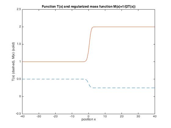
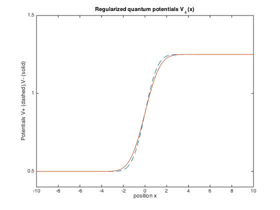
Figure 2. On the top: the function $T(x)$ defined by (8.4) and the corresponding regularized mass $\mathcal{M}(x)=1/(2T(x))$ replacing the discontinuous mass introduced in (8.1) with $m_{l}<m_{r}$. On the bottom, the regularized potentials $\mathcal{V}_{\pm}(x)$ defined by (8.5).

Let us now establish the quantum phase space portraits of the Hamiltonian operator $A_{H}$ along the lines given by (7.5). We obtain the following smooth regularisation of the original $H(q,p)$:

(8.9) $$\check{H}(q,p)=T(q)\,p^{2}+\frac{2}{\sigma_{\ell}^{2}}\,T(q)+\frac{V_{0}}{2}\,\mathrm{Erfc}\left(-\frac{\sigma_{\eth}}{\sqrt{2}}\,q\right)\equiv T(q)\,p^{2}+\mathcal{V}_{\mathrm{sc}}(q)\,.$$

We note the factor $2$ appearing in the first term of the semi-classical potential and which is not present in the quantum potential.

9. Conclusion

We have outlined a procedure transforming a classical model for a physical system into one of its quantum versions by using a combination of symmetry principle, integral calculus on operators and functions, with a (quasi-) probabilistic interpretation as a guideline. The procedure is applied to the motion of a variable mass particle on the line, and illustrated with the elementary case of a step potential. The extension to more realistic cases is actually straightforward, save for unescapable technicalities. We would like to promote the idea that in the building of a quantum model, supposed to agree better with observation, one can start from a classical rough model or sketch, allowing mathematical idealisations, smoothness, infinities, discontinuities, singularities, and then correct the quantum outcome by using the large freedom we dispose with the choice of a certain coarse-graining determining the procedure. The considered symmetry in the present work was the projective representation of translations in the Euclidean plane, as much rich than it is simple. Clearly, the method can be adopted in considering many other phase space geometries, e.g., half-plane for the motion on the half-line [24, 25], cylinder for the motion on the circle [26], $\mathbb{R}^{2}_{\ast}\times\mathbb{R}^{2}$ for the motion in a punctured plane [27], etc. A promising development of the method [28] is to start from $\mathbb{R}^{2n}$ as a phase space, then extend the method presented in this paper by using the Weyl-Heisenberg projective translationnal symmetry of $\mathbb{R}^{2n}$, and restrict the quantization to all observables with support in a fixed smooth or singular manifold in $\mathbb{R}^{n}$.

Acknowledgments

The author is indebted to the Centro Brasileiro de Pesquisas Físicas (Rio de Janeiro) and CNPq Agency (Brazil), and the Institute for Research in Fundamental Sciences (IPM, Tehran) for financial support. He also thanks the CBPF and the IPM for hospitality. He is grateful to Evaldo M.F. Curado (CBPF) for valuable comments on the content of this work.

References

- [1] E. Inönü and E. Wigner, Representations of the Galilei group, Nuovo Cimento 9, (1952) 705-718.
- [2] A. S. Wightman, On the localizibility of quantum mechanical systems. Rev. Modern Phys. 34 (1962) 845-872.
- [3] F. A. Berezin, Quantization, Mathematics of the USSR-Izvestiya 8(5) 1109-1165 (1974); General concept of quantization; Commun. Math. Phys. 40 153-174 (1975).
- [4] S. T. Ali and M. Engliš, Quantization methods: a guide for physicists and analysts, Rev. Math. Phys. 17 (2005) 391.
- [5] N. P. Landsman, Between classical and quantum, in J. Earman, & J. Butterfield (Eds.), Philosophy of physics, Handbook of the philosophy of science (Vol. 2). Amsterdam: Elsevier (2006). arXiv:quant-ph/0506082
- [6] M. Combescure and D. Robert, Coherent States and Applications in Mathematical Physics, Theoretical and Mathematical Physics, Springer-Netherlands.
- [7] M. de Gosson, Born-Jordan Quantization, Fundamental Theories of Physics, 182 Springer, Cham.
- [8] H. Bergeron, J.P. Gazeau, A. Youssef, Are the Weyl and coherent state descriptions physically equivalent? Phys. Lett. A 377 (2013) 598-605
- [9] A. O. Barut and R. Ra̧czka, Theory of Group Representations and Applications (PWN, Warszawa, 1977).
- [10] J. von Neumann, Die eindeutigkeit der Schröderschen Operatoren, Math. Ann., 104 570-578 (1931); Mathematical foundations of quantum mechanics (Princeton University Press, 1955).
- [11] A.M. Perelomov, Generalized Coherent States and Their Applications (Springer, Berlin, 1986).
- [12] H. Bergeron and J.-P. Gazeau, Integral quantizations with two basic examples, Annals of Physics (NY) 344 43-68 (2014); arXiv:1308.2348 [quant-ph, math-ph]
- [13] H. Bergeron, E.M.F. Curado, J.-P. Gazeau, and Ligia M.C.S. Rodrigues, Weyl-Heisenberg integral quantization(s): a compendium (2017) arXiv:1703.08443 [quant-ph]
- [14] An apodization function (also called a tapering function or window function) is a function used to smoothly bring a sampled signal down to zero at the edges of the sampled region.
- [15] L. Cohen, Generalized Phase-Space Distribution Functions, J. Math. Phys. 7 (1966) 781-786.
- [16] L. Cohen, The Weyl Operator and its Generalization, Pseudo-Differential Operators: Theory and Applications 9, Birkhaüser, 2013.
- [17] B. S. Agarwal and E. Wolf, Calculus for Functions of Noncommuting Operators and General Phase-Space Methods in Quantum Mechanics, Phys. Rev. D 2 (1970) 2161 (I), 2187 (II), 2206 (III).
- [18] N. I. Akhiezer and I. M. Glazman, Theory of Linear Operators in Hilbert Space (Pitman, 1981).
- [19] J.-M Lévy-Leblond, The pedagogical role and epistemological significance of group theory in quantum mechanics, Riv. Nuovo Cimento 4 99-143 (1974).
- [20] J. M. Lévy-Leblond, Elementary quantum models with position-dependent mass, Eur. J. Phys. 13 215-218 (1992).
- [21] J. M. Lévy-Leblond, Position-dependent effective mass and Galilean invariance, Phys. Rev. A 52 1845-1849 (1995).
- [22] E. Cordero, M. de Gosson, and F. Nicola, On the Invertibility of Born-Jordan Quantization; arXiv:1507.00144 [math.FA]
- [23] M. Abramowitz and I.A. Stegun (Eds.), Handbook of Mathematical Functions with Formulas, Graphs, and Mathematical Tables, 9th printing (Dover, New York, 1972).
- [24] J.-P. Gazeau and R. Murenzi, Covariant Affine Integral Quantization(s), J. Math. Phys. 57 (2016) 052102; arXiv:1512.08274 [quant-ph]
- [25] C.R. Almeida, H. Bergeron, J.-P. Gazeau, and A.C. Scardua, Three examples of quantum dynamics on the half-line with smooth bouncing, Annals of Physics (NY), in press and online (2018); arXiv:1708.06422v1 [quant-ph]
- [26] R. Fresneda, J.-P. Gazeau, and D. Noguera, Quantum localisation on the circle, submitted; arXiv:1708.03693 [quant-ph]
- [27] J.-P. Gazeau, T. Koide and R. Murenzi, More quantum repulsive effect in rotating frame, EPL 118 (2017) 50004.
- [28] J.-P. Gazeau and T. Koide, Quantum motion on the half-line from Weyl-Heisenberg integral quantization, in preparation.