Meterwavelength Single-pulse Polarimetric Emission Survey IV: The Period Dependence of Component Widths of Pulsars.

Abstract

The core component width in normal pulsars, with periods ($P$) $>$ 0.1 seconds, measured at the half-power point at 1 GHz has a lower boundary line (LBL) which closely follows the $P^{-0.5}$ scaling relation. This result is of fundamental importance for understanding the emission process and requires extended studies over a wider frequency range. In this paper we have carried out a detailed study of the profile component widths of 123 normal pulsars observed in the Meterwavelength Single-pulse Polarimetric Emission Survey at 333 and 618 MHz. The components in the pulse profile were separated into core and conal classes. We found that at both frequencies the core as well as the conal component widths versus period had a LBL which followed the $P^{-0.5}$ relation with a similar lower boundary. The radio emission in normal pulsars have been observationally shown to arise from a narrow range of heights around a few hundred kilometers above the stellar surface. In the past the $P^{-0.5}$ relation has been considered as evidence for emission arising from last open dipolar magnetic field lines. We show that the $P^{-0.5}$ dependence only holds if the trailing and leading half-power points of the component are associated with the last open field line. In such a scenario we do not find any physical motivation which can explain the $P^{-0.5}$ dependence for both core and conal components as evidence for dipolar geometry in normal pulsars. We believe the period dependence is a result of an yet unexplained physical phenomenon.

1 Introduction

The coherent radio emission from pulsars are believed to arise due to growth of instabilities in relativistic strongly magnetized plasma outflowing along open dipolar magnetic field lines well inside the light cylinder, however the underlying physical mechanism that excites the coherent radio emission is still unidentified (see e.g. Michel, 1982; Beskin et al. , 1993; Asseo & Melikidze, 1998; Melikidze et al. , 2000; Melrose, 2017; Mitra, 2017). The radio pulsar population can be roughly divided into two groups based on their periods, millisecond pulsars with periods much less then 100 milliseconds and normal pulsars with periods longer than this value. The presence of dipolar magnetic fields in the emission region is motivated by the widths of the profile and specific components which exhibit a dependence on the period ($P$). In this work we take a critical look into this argument utilizing the measured profiles of 123 normal pulsars with periods greater than 0.1 seconds observed in the Meterwavelength Single-pulse Polarimetric Emission Survey (MSPES, Mitra et al. , 2016b; Basu et al. , 2016). Only for pulsars with periods larger than 0.1 second will an emission region that is located roughly 500 km above the neutron star (Blaskiewicz et al. , 1991; von Hoensbroech & Xilouris, 1997; Kijak & Gil, 1997; Mitra & Li, 2004; Weltevrede & Johnston, 2008; Krzeszowski et al. , 2009; Mitra & Rankin, 2011) be largely unaffected by strong field line distortions (Dyks, 2008).

The periodic radio emission in normal pulsars has typical duty cycles of $\sim$ 10% and the single pulses often consist of smaller structures called subpulses. In some cases the subpulses appear at the same phase within the pulse window while in others they jitter or systematically move in phase. When the single pulses are averaged for a few thousand periods a stable integrated profile is formed which is composed of one or more distinct gaussian shaped components. These components are formed due to the averaging of subpulses but their properties like width and location might differ from the individual subpulses depending on the subpulse dynamics. The physical origin of the subpulses in single pulses are still unknown. The most notable radio emission model that predict the presence of subpulses is that of Ruderman & Sutherland (1975) where the subpulses are associated with radiation generated from isolated plasma columns. The plasma columns are generated due to sparking discharges in an inner accelerating region characterised by high electric fields just above the polar cap. The formation of subpulses have also been speculated to arise due to non-radial oscillations in neutron star (Clemens & Rosen, 2004) or due to development of instability in the outflowing plasma (Fung et al. , 2006). This motivates the study of average subpulse properties in a large number of pulsars to constrain the formation of these emission structures.

The number of components in the profiles are seen to vary in the pulsar population. The full widths of the profiles usually exhibit a frequency evolution where the widths are seen to decrease with increasing frequency and the number of components often change with frequency in a systematic manner. The profiles are highly polarized and the linear polarization position angle (PPA) executes a S-shaped traverse across them. The rotating vector model (RVM, Radhakrishnan & Cooke, 1969) is used to explain the shape of the PPA traverse where beamed emission arises from regions of diverging, but not necessarily dipolar magnetic field lines with the PPA traverse corresponding to the change in the field line planes. In addition, the PPA traverse is also affected by the observer’s line of sight cut through the pulsar emission beam. If the diverging magnetic field lines are ascribed to a star centered global dipolar magnet, the RVM is expressed as a function of the dipolar geometrical angles, viz. the angle between the rotation axis and the dipole magnetic axis, $\alpha$, and the angle between the dipole magnetic axis and the observer’s line of sight $\beta$. The RVM has been shown to fit the PPA traverse in normal pulsars very well indicating the emission to originate from dipolar magnetic fields (Everett & Weisberg, 2001; Mitra & Li, 2004). On the other hand these fits are very often unsuitable for estimates of the angles $\alpha$ and $\beta$ when data exhibit large error bars on PPA. The fit residuals become strongly correlated and good constraints for an unique solution are absent. However, the steepest gradient (SG) point of the PPA which lies in the plane containing the rotation and dipole magnetic axis can often be used to provide the necessary additional constraint

$$R_{ppa}=\sin(\alpha)/\sin(\beta).$$ (1)

where $R_{ppa}$ corresponds to the slope of the PPA at SG, for a more accurate determination of $\alpha$ and $\beta$.

A number of studies in the literature details the interplay between the magnetospheric plasma with the field configuration, including the polar cap structure (Bai & Spitkovski, 2010), the structure of the large scale magnetic field and plasma (Philippov & Spitkovsky, 2014; Philippov et al. , 2015), the location of discharge regions and plasma sources (Chen & Beloborodov, 2014), the dynamics of discharge regions (Szary et al. , 2015; Timokhin & Arons, 2013) and propagation effects (Petrova & Lyubarskii, 2000; Hakobyan & Beskin, 2014). Additionally, the outflowing plasma in the rotating magnetosphere can also lead to effects like abberation and retardation (A/R hereafter), magnetic field sweepback, etc. These can potentially distort the shape of the PPA traverse, yet the RVM corresponding to a relatively simplified model of empty pulsar magnetosphere are excellent fits to the PPA in normal pulsars (Everett & Weisberg, 2001; Mitra & Li, 2004). Several studies have shown that if the radio emission detaches from the magnetosphere at heights of $h_{em}<0.1R_{LC}$, where $R_{LC}$ = $pc/2\pi$ is the light cylinder radius, the A/R effects are the only discernible observable distortion affecting the PPA traverse (Blaskiewicz et al. , 1991; Hibschman & Arons, 2001; Dyks, 2008; Craig & Romani, 2012; Kumar & Gangadhara, 2012a, b, 2013). In such a scenario if the radio emission detaches at a constant height across the pulsar profile, the A/R effect can be approximated as a positive shift in longitude, $\Delta\phi$, between the center of the total intensity profile and the SG point of the PPA traverse, which is linearly dependent on $h_{em}$. This can in turn be used to estimate the emission heights as $h_{em}=(c/4)(\Delta\phi/360\arcdeg)P$ km. Using the above relation a number of observations have found the radio emission in normal pulsars to detach from the magnetosphere around $h_{em}\sim$ 100–1000 km, which is well below 0.1$R_{LC}$ (Blaskiewicz et al. , 1991; von Hoensbroech & Xilouris, 1997; Mitra & Li, 2004; Weltevrede & Johnston, 2008; Mitra & Rankin, 2011). It should be noted that the excellent fits of the PPA traverse with the RVM indicates that the emission region across the pulse profile originate from similar heights, since significant changes in emission height can distort the PPA traverse (see for e.g. Mitra & Seiradakis (2004)). The radio emission is excited in the plasma at a certain height $h_{g}$, where $h_{g}<h_{em}$, and then it propagates in the plasma and eventually detaches at $h_{em}$. The plasma properties in the propagation region can influence the properties of the radio emission and several conflicting models exist in the literature which either suggest that the radiation is unaffected by propagation (Mitra et al. , 2009; Melikidze et al. , 2014) or that the radiation is modified due to the propagation effect (Petrova & Lyubarskii, 2000; Hakobyan & Beskin, 2014). However, the observational constraints from pulsar radiation can still be used to study the magnetospheric structure at the detachment point $h_{em}$. At these heights the estimates of the locus of the open dipolar field lines suggest the emission region to be close to a circular patch (Arendt & Eilek, 2002; Dyks & Harding, 2004). This motivates the idea of the emission components in the pulsar profile of normal pulsars to originate from an emission beam radiating approximately at a constant height and the angular dimensions of the emission component and beams can be constrained by spherical geometry.

The components can be separated into core and conal types which exhibit distinct frequency evolution as well as different polarization characteristics, with the core always centrally located within the profile. The emission beam in pulsars has been conceptualized as a circularly symmetric structure consisting of a central core component surrounded by concentric rings of conal components (Rankin, 1990, 1993a, 1993b, R90 and R93 hereafter). The principal justification for the above picture is provided by the different profile shapes in the pulsar population which can be categorized into five distinct classes. The five component profiles consisting of a central core component flanked by two pairs of inner and outer conal outriders are classified as Multiple (M) class. There are two classes of three component profiles namely core Triple (T) which has a central core component along with one pair of conal outriders and the conal Triple (_cT) where all the three components are conal. The two component profiles correspond to conal Double (D) class. Finally, the single component profiles are classified either as Core Single (S_t) or the Conal Single (S_d) classes. It is believed that the different profile classes arise due to different line of sight cuts through the emission beam and is therefore dependent on the pulsar geometry, with the beam radius ($\rho^{\nu}$) given as (Gil et al. , 1984) :

$$\sin^{2}(\rho^{\nu}/2)=\sin(\alpha)\sin(\alpha+\beta)\sin^{2}(W^{\nu}/4)+\sin^{2}(\beta/2)$$ (2)

where $W^{\nu}$ is the estimated profile width at frequency $\nu$. Further, by assuming $W^{\nu}$ to be bound by the last open dipolar field lines, an estimate of the emission height ($h^{\nu}$) above the neutron star polar cap can be computed as:

$$h^{\nu}=10P\left(\frac{\rho^{\nu}}{1.23\arcdeg}\right)^{2}{\rm km}$$ (3)

where the radius of the opening angle of the polar cap at the stellar surface ($R$ = 10 km) corresponds to $1.23\arcdeg$. As discussed above the pulsar geometry, angles $\alpha$ and $\beta$, cannot be constrained using the RVM. Hence, $h^{\nu}$ cannot be calculated with any certainty using equations (2) and (3).

R90 established a dependence of the core component widths with pulsar period which enabled an alternative scheme for estimating the pulsar geometry. The widths measured at 1 GHz $W_{core}^{1{\rm GHz}}$ (estimated at 50% of peak intensity) showed the presence of a lower boundary line (LBL) scaling as $2.45\arcdeg P^{-0.5}$. R90 further established that core widths for several inter-pulsars (where $\alpha\sim 90\arcdeg$) lay along the LBL. It should be noted that pulsars with core components have the line of sight passing centrally through the emission beam and hence their $\beta$ is small. Incidentally, the boundary value $2.45\arcdeg$ is very close to the diameter of the dipolar opening angle at the stellar surface. It was postulated that $W_{core}^{1{\rm GHz}}$ encompasses the pulsar polar-cap bounded by last open dipolar field lines. The pulsars with the measured widths above the line corresponds to non-orthogonal rotators with $\sin\alpha<1$. This allowed an independent estimation of the angle $\alpha$ from $W_{core}^{1{\rm GHz}}$ using the relation:

$$W_{core}^{1{\rm GHz}}=2.45P^{-0.5}/\sin\alpha$$ (4)

R93 expanded the above idea to estimate the geometry in a large number of pulsars with core components. The conal separation in profile classes T and M, with prominent core components, were also measured. It was proposed that the inner and outer cones originate at different heights and encompass the entire open field line region. The half-power points of inner and outer conal pairs ($W_{in,out}^{1{\rm GHz}}$) also enabled the estimation of the radius of the opening angle ($\rho_{in,out}^{1{\rm GHz}}$) for the conal rings as :

$$\rho_{in}^{1{\rm GHz}}=4.3\arcdeg P^{-0.5};\rho_{out}^{1{\rm GHz}}=5.8\arcdeg P^{-0.5}$$ (5)

R93 estimated the inner and outer cones to arise from heights (eq.3) of roughly 130 km and 220 km respectively. The method of analysing profile widths and components by R90, R93 has an underlying assumption that all relevant widths arise from the entire open field line region with an emphasis on the core, which is believed to fill up the entire polar cap, the inner and outer conal pairs, once again representing the entire open field line regions, etc. There are no provisions for interpreting the widths of the individual components in these schemes.

The above picture of the radio emission is difficult to reconcile with recent observations where emission heights of the core and conal components is emitted from similar heights in the same pulsar. It has now been shown in many M and T class pulsars that the core and conal emission originates from similar heights (Mitra et al. , 2007; Mitra & Rankin, 2011; Smith et al. , 2013; Mitra et al. , 2016a). In this context the $P^{-0.5}$ scaling relation between $W_{core}^{\nu}$ and $\rho^{\nu}$ needs careful consideration. If we assume $\beta$ to be small and $\alpha>>\beta$ (which is justified for central cuts with core emission), the radius of the emission beam in eq.(2) can be approximated as :

$$\rho^{1{\rm GHz}}=\sqrt{4\sin^{2}(\alpha)\sin^{2}(W^{1{\rm GHz}}/4)+\beta^{2}}.$$ (6)

Now substituting sin($\alpha$) in terms of core width (eq.4, which introduces the $P^{-0.5}$ dependence) and $\beta$ in terms of sin($\alpha$) and $R_{ppa}$ (eq.1) the emission beam is estimated as:

$$\rho^{1{\rm GHz}}=2.45P^{-0.5}F$$ (7)

where the factor $F$ is given by

$$F=\sqrt{\left(\frac{4\sin^{2}(W^{1{\rm GHz}}/4)}{(W_{core}^{1{\rm GHz}})^{2}}+\frac{1}{({R_{ppa}W_{core}^{1{\rm GHz}}})^{2}}\right)}$$ (8)

As is clear from the above exercise the $P^{-0.5}$ dependence in $\rho^{1{\rm GHz}}$ is transferred from the $P^{-0.5}$ dependence of the core width and is only preserved if the factor $F$ does not have any period dependence.

To further investigate this in M and T class profiles with prominent core and conal components we recall that $R_{ppa}$ is usually large and hence the second term in eq.(8) can be ignored. Now if we assume that the total width $W^{1{\rm GHz}}$ to be small, $F$ can be approximated as

$$F\sim W^{1{\rm GHz}}/2W_{core}^{1{\rm GHz}}.$$ (9)

The total width $W^{1{\rm GHz}}$ can be separated into individual components:

$$W^{\nu}=W_{core}^{\nu}+\sum_{i}W_{cone,i}^{\nu}+\sum_{j}\delta W_{j}^{\nu}$$ (10)

where $W_{cone,i}^{\nu}$ is the width of the $i^{th}$ conal component, $\delta W_{j}^{\nu}$ is the $j^{th}$ separation between adjacent components with the summation extending over all conal components as well as the respective separation between adjacent components. Now, For the factor $F$ to be period independent $W^{1{\rm GHz}}$ should also show a $P^{-0.5}$ dependence. This further implies that along with $W_{core}^{\nu}$, the $W_{cone,i}^{1{\rm GHz}}$ and $\delta W_{j}^{1{\rm GHz}}$ should also have $P^{-0.5}$ dependence.

To the best of our knowledge no such study exists in the literature connecting the conal components widths with the pulsar period. Only some hints of this effect have been discussed in Maciesiak et al.  (2011a, b, 2012) and Mitra et al.  (2016b). In these works a distribution of total half-power width of all available profiles with period found a LBL which scaled as $P^{-0.5}$. Since no particular profile class was selected to obtain this relation, a LBL might exist for both core and conal widths following a similar $P^{-0.5}$ relation. In this paper, we use the MSPES data to carry out a detailed study of the profile component widths and investigate their dependence on period. Furthermore, we explore the implications of the period dependence of component widths on the dipolar geometry.

2 Component Width Analysis

The principal analysis involved estimating the relevant widths of the components and the separation between adjacent components. Generally, the widths can be directly measured in the integrated profiles where the components are clearly distinguished. But in some pulsars, due to phenomenon like subpulse drifting, the subpulses are seen to systematically drift in phase across the pulse window. It is also possible that in the same pulsar different components might be associated with different subpulse dynamics resulting in different widths. In such cases a more accurate estimate of the emission properties are possible by correcting for the subpulse motion across the pulse window and form an average component from selected single pulses.

We used the MSPES data at 333 and 618 MHz for 123 pulsar with high quality single pulses for this purpose (Mitra et al. , 2016b). Specialized techniques were needed to enhance the individual components using precisely selected single pulses to make the relevant components more prominent. We have employed three different techniques (mentioned below) to generate the most prominent realization of each component in the pulsar profile. The components once identified were classified into core and the conal types and their respective widths at each frequency were measured at the 50% level of the peak intensity ($W_{core}$ and $W_{cone}$). The 50% level was selected as a representative width of the component since any lower level (like 25% or 10%) are usually contaminated by the adjacent components making the estimation difficult in a large number of components.

2.1 Identifying Profile Components

Here we discuss the three different techniques that were used to measure component widths using the single pulse analysis. Before the single pulses were averaged the baseline level from each single pulse was removed and the integrated profile peaks were normalized to unity after the components were formed.

1. Integrated Profile
In this method the average profiles were produced with an additional modification of selecting only significant single pulses with peaks above five times the rms noise level of the off-pulse baseline. This enhanced the signal to noise ratio (SNR) of the components especially in pulsars which showed nulling (Basu et al. , 2017). This technique was most widely used in this work with 89 pulsars at 333 MHz and 112 pulsars at 618 MHz where the components were characterized. Figure 1 illustrates the integrated profile for the pulsar J0304+1932 where we used this method.

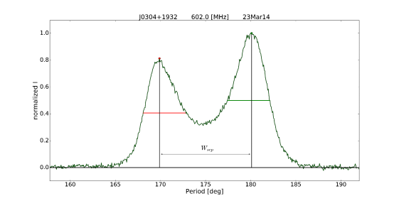
Figure 1: The figure shows the measured width ($W_{cone}$) for the conal components and the separation ($W_{sep}$) between the peaks in the pulsar J0304+1932. The green and red points on the graph correspond to the peaks of the individual components, while the horizontal lines of the same color correspond to the measured component widths at 50% level of the peak. The widths were estimated using the integrated profile (see section 2.2). The black vertical lines indicate the measured separation between the peaks.

2. Averaging Subpulses
In this method we separated out the components in 2 pulsars at 333 MHz and 3 pulsars at 618 MHz which appear merged in the average profile. The subpulses corresponding to the components were seen to separate out in the single pulses and with jittering in phase. The peaks of each component were identified in the average profile using a peak detection technique. Template windows of width 2.45°$P^{-0.5}$ and center phase corresponding to the component peaks were set up. Any single pulse exceeding three times the off-pulse noise levels in each of these windows were considered for the respective average components. In addition a further criterion for averaging was that the peak of the subpulse within the window was close to the central phase (within 5-10 longitude bins). Finally, all relevant single pulses were averaged to generate a profile with the relevant component prominently detected. A separate profile for each individual component was generated in this technique. In figure 2 the results of this exercise for the pulsar J1745$-$3040 is shown, where the second component becomes prominent after applying this technique. The leading component of this pulsar do not form a fully formed conal component, resembling a pre-cursor (Basu et al. , 2015), and has not been used for component width analysis.

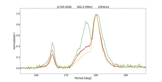
Figure 2: The figure shows the component estimation in the pulsar J1745$-$3040. The black curve shows the integrated profile. The yellow, green and red curves correspond to the profiles used to measure the first, second and third component using the second method described in section 2.1. The second component could be clearly distinguished only after using these specialized techniques. The leading component is made up of sporadic emission and is unlikely to be a fully formed conal component. The width of the component is smaller than the typical conal width and marked separately as a yellow dot in figure 5.

3. Averaging Peaks in Window
This technique was used to estimate the components in 20 pulsars at 333 MHz and 19 pulsars at 618 MHz. This was mainly useful for subpulses which showed prominent drift bands and systematic shift in phase within the pulse window. In order to measure the component widths a technique was devised to average the peaks appearing at similar phases. Inside the profile windows, 5-10 bins wide, were set up and were spread contiguously across the whole profile. All significant subpulses (peak intensity greater than five times the baseline rms) with peaks within the relevant window were averaged to form a profile corresponding to that window. All such profiles with at least $10\%$ of the total pulses were used for subsequent analysis. The profile separated out into individual components as shown in figure 3 for the pulsar J2305+3100. By this method we generated several representative profiles which had one or components. We measure the widths of all these components and produced an average component width for the pulsar. Similarly, we estimated the separation between components for all relevant cases and estimated an average $W_{sep}$.

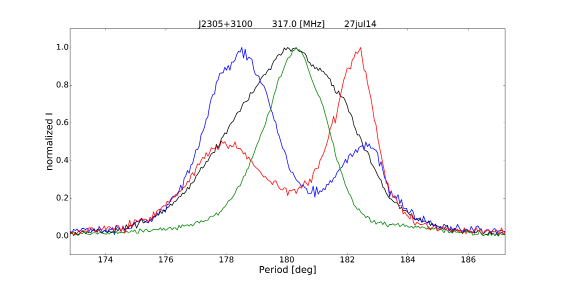
Figure 3: This figure demonstrates the use of the third method described in section 2.1 for the pulsar J2305+3100. This method was used for pulsars showing subpulse drifting with prominent drift bands. The components were well separated at the single pulse level but shifted across the window giving a smeared average profile (black line). As shown by the red, blue, green profiles, our technique was successful in separating the components and estimating their widths as well as the separation between them.

2.2 Measuring Component Widths

Using the analysis scheme discussed above we were able to develop the best possible profile for the individual components. However, it was not always possible to clearly separate out the components in all cases. But in many of these cases it was still possible to find an estimate of the widths using certain fitting procedures. We employed three different techniques for measuring the 50% widths of the components which we describe below.

1. Full Width
This was the commonly used technique in our analysis where the 50% of peak intensity on either side of the component could be clearly measured (see figure 1). The estimated width was the separation between the 50% points on either side of the peak. A total of 99 component widths at 333 MHz and 123 widths at 618 MHz were measured using this technique.

2. Half Width
This method was used to estimate the widths of 76 components at 333 MHz and 82 components at 618 MHz. This was utilized when the peaks were clearly seen but one side was not well separated from the adjacent component. The separation of the peak from the 50% point of the well resolved side was calculated and multiplied by two, to obtain an approximate estimate of the component width.

3. Gaussian Fits
In a small number of cases, 11 components at 333 MHz and 20 components at 618 MHz, the peak was not clearly seen. In such cases a Gaussian function was fitted to the component and the full width at half maximum (FWHM) of the Gaussian was used as an estimate of the width. However, the Gaussian fit is not always an accurate model for the subpulses and the widths in such cases should be used with caution.

2.3 Separation Between Adjacent Components

The separation between adjacent components ($W_{sep}$) in profiles with more than one component was calculated. We used the peak positions estimated in the previous subsection for each component to find the separation between them (see figure 1 for a schematic). In some cases the exact location of the peak was uncertain due to lower sensitivity of the emission and a Gaussian fit was used to approximate the peak position.

2.4 Error Estimation

The error ($\sigma$) in estimating the component width was evaluated as (Kijak & Gil, 2003):

$$\sigma=res\times\sqrt{1+\left(\frac{rms}{I}\right)^{2}},$$ (11)

where $res$ is the longitude resolution in degrees, $rms$ corresponds to the baseline noise levels and $I$ is the measured signal, in our case $I$ corresponds to peak intensity. In case of the separation between components, the error in estimating each peak position was determined and the overall error was calculated by propagating the individual errors.

3 Results

In Table LABEL:tabela we have presented the results of our analysis for the 123 pulsars observed at two frequencies 333 MHz and 618 MHz. We have determined the number of profile components and its classification at each frequency and measured their widths wherever possible. In addition we have also determined the separation between adjacent components. Additionally, the table also lists the measurement schemes employed for every component (see section 2.1 and 2.2 for details).

3.1 Component Widths and Separation

The widths were measured for 418 components in total, including 191 widths at 333 MHz and 227 widths at 618 MHz. There were 117 $W_{core}$ in total out of which 54 $W^{333{\rm MHz}}_{core}$ and 63 $W^{618{\rm MHz}}_{core}$. Correspondingly, we measured 301 $W_{cone}$ out of which 137 $W^{333{\rm MHz}}_{cone}$ and 164 $W^{333{\rm MHz}}_{cone}$. In addition $W_{sep}$ had 217 measurements, with 100 $W^{333{\rm MHz}}_{sep}$ and 117 $W^{618{\rm MHz}}_{sep}$. The period dependence of $W_{core}$, $W_{cone}$ and $W_{sep}$ in logarithmic scales for each frequency are shown in figure 4,5. There are four separate plots corresponding to all the measured widths, $W_{all}$ (top left panel), all $W_{sep}$ (top right panel), $W_{core}$ (bottom left panel) and $W_{cone}$ (bottom right panel). In each case it is clear that a lower boundary exists for the widths as well as the separations, though the boundary is less tightly constrained for $W_{sep}$. In addition figure 6 separately shows the conal widths estimated for the subpulse drifting pulsars using method 3 in section 2.1. It is seen that the boundary estimates are not affected by these widths. A statistical approach using quantile regression (see appendix A for a discussion on quantile regression) was employed to determine the LBL in each case.

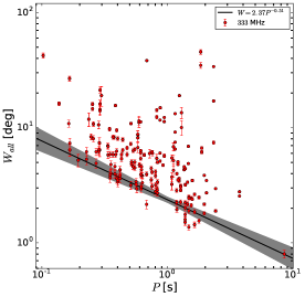
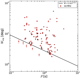
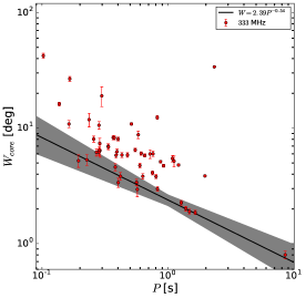
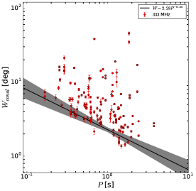
Figure 4: In this figure we plot the widths $W_{all}$, $W_{core}$ and $W_{cone}$ as well as the separation $W_{sep}$ as a function of the pulsar period ($P$) at 333 MHz. On the upper left panel both core and conal components are shown together whereas on the lower left panel the core component is plotted separately and likewise for the conal components on the lower right panel. On the upper right panel $W_{sep}$ is plotted against $P$. The black line in each plot is our estimate of the lower boundary line using quantile regression (see section 3.2) with the grey area representing the errors from our fits. In the case of $W_{sep}$ we were not able to constrain the lower boundary line using the fitting process and the boundary was obtained by assuming a $P^{-0.5}$ dependence.

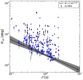
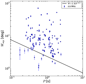
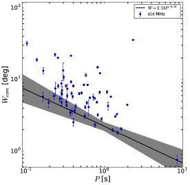
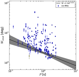
Figure 5: In this figure we plot the widths $W_{all}$, $W_{core}$ and $W_{cone}$ as well as the separation $W_{sep}$ as a function of the pulsar period ($P$) at 618 MHz. The yellow point corresponds to the leading component in PSR J1745$-$3040 which is not a fully formed conal component and has a lower width. On the upper left panel both core and conal components are shown together whereas on the lower left panel the core component is plotted separately and likewise for the conal components on the lower right panel. On the upper right panel $W_{sep}$ is plotted against $P$. The black line in each plot is our estimate of the lower boundary line using quantile regression (see section 3.2) with the grey area representing the errors from our fits. In the case of $W_{sep}$ we were not able to constrain the lower boundary line using the fitting process and the boundary was obtained by assuming a $P^{-0.5}$ dependence.

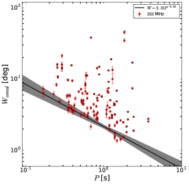
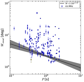
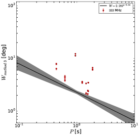
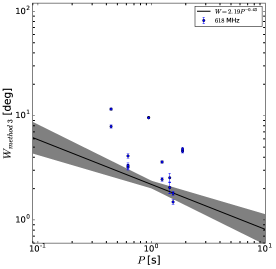
Figure 6: In this figure we separately show that the values of the conal widths for pulsars showing subpulse drifting, measured using method 3 in section 2.1, do not dominate the boundary line estimates. The top figures show the conal width distributions without the drifting widths at 333 MHz (top left panel) and 618 MHz (top right panel) respectively. The boundary line is estimated in each case using the method of quantile regression and is identical to the overall estimates within measurement errors. The bottom panels show the drifting widths at 333 MHz (bottom left panel) and 618 MHz (bottom right panel) respectively. The lower boundary could not be estimated statistically for just the drifting cases due to the small number of measurements. However, the lower boundary from figures 4 and 5 is shown in these figures. It is seen that the estimated widths do not occupy the boundary line but are widely distributed.

3.2 The Lower Boundary Line

Table 1: THE LOWER BOUNDARY LINE: $W$ = $W_{B}$°$P^{-b}$

		333 MHz		618 MHz		Both Freq.
		$W_{B}$	$b$	$W_{B}$	$b$	$W_{B}$	$b$
	$W_{core}$	2.39$\pm$0.26	0.54$\pm$0.11	2.23$\pm$0.30	0.51$\pm$0.13	2.28$\pm$0.19	0.51$\pm$0.08
Comp. Width	$W_{cone}$	2.28$\pm$0.15	0.54$\pm$0.10	2.19$\pm$0.17	0.43$\pm$0.11	2.24$\pm$0.11	0.49$\pm$0.07
	$W_{all}$	2.37$\pm$0.13	0.51$\pm$0.07	2.16$\pm$0.14	0.49$\pm$0.08	2.25$\pm$0.09	0.51$\pm$0.05
$W_{sep}$		2.81	0.5	2.35	0.5	2.66	0.5
Prof. Width		3.30	0.5	2.97	0.5	2.99	0.5

The LBL is of the form $W_{B}P^{-b}$, where $W_{B}$ is the boundary width and $b$ the period dependence. Table 1 shows the estimates of the LBL for each category of measured widths. The first row represents the estimates of LBL for $W_{core}$, $W_{cone}$ and $W_{all}$ at each frequency using quantile regression. The $b$ value in each case is close to $0.5$ suggesting that the $P^{-0.5}$ dependence is consistent for the component widths. We use the period dependence to exhibit the $P^{-0.5}$ relation in subsequent discussions as a close approximation to the measured dependence. The boundary value $W_{B}$ was lower than 2.45° which was the previously estimated boundary for the core widths at 1 GHz. The frequency evolution of component widths suggests that the measurements at 333 MHz and 618 MHz should be greater than the corresponding values at 1 GHz. However, the measured $W_{B}$ at 333 MHz was greater than at 618 MHz in accordance with our expectations. Assuming a frequency dependence of component width ($\propto\nu^{\gamma}$), the estimated $\gamma$ is -0.15$\pm$0.01 and the boundary at 1 GHz is $W_{B}^{1{\rm GHz}}$ = 2.01$\pm$0.15° which is smaller than the previous estimates. In addition, the results also show that $W_{B,core}$ (2.28$\pm$0.19°) and $W_{B,cone}$ (2.24$\pm$0.11°) are similar. There was a possibility that the lower boundary line was affected by the drifting widths measured using method 3 in section 2.1. To eliminate this possibility the boundary lines were estimated separately by removing the drifting widths. The estimated conal boundary line for the entire population without the drifting widths are $W_{B,cone,nd}^{333{\rm MHz}}$ = 2.16$\pm$0.12°and $W_{B,cone,nd}^{618{\rm MHz}}$ = 2.23$\pm$0.14°, respectively. These values are similar to the overall boundaries (within measurement errors) and show that the widths of the drifting components do not bias the boundary line.

The statistical method was unable to constrain the period dependence in $W_{sep}$. We nonetheless estimated a boundary for these quantities as well by assuming a $P^{-0.5}$ dependence and estimating boundary below which only 10% points were present (the 0.1 quantile level, see appendix). The estimated boundaries of $W_{sep}$ at 333 MHz, 618 MHz and all combined are shown in second row of Table 1. Additionally, the lower boundary for $W_{prof}$ in the average profiles (Mitra et al. , 2016b) was also estimated at the 0.1 quantile level (assuming a $P^{-0.5}$ dependence) and are shown in third row of Table 1.

4 Discussion

4.1 Period dependence of Component widths

It has been shown observationally that the radio emission in normal pulsars originate at heights $R_{E}\sim$ 500 km (Blaskiewicz et al. , 1991; von Hoensbroech & Xilouris, 1997; Mitra & Li, 2004; Weltevrede & Johnston, 2008; Mitra & Rankin, 2011). It has also been shown in several cases that both the core and conal components arise from similar heights within the pulsar magnetosphere (see Table 2 in Mitra et al. , 2016a). In addition we have now shown that both the core and conal components have similar LBL which shows a $P^{-0.5}$ dependence. Hence, the average emission beam in normal pulsars can be imagined to consist of a central core component surrounded by conal components around similar heights as shown schematically in figure 7. It has been argued in earlier works (e.g. R90, Maciesiak et al. , 2012) that the $P^{-0.5}$ is an indication of the evolution of the components along the dipolar field lines since the open field line regions in dipolar magnetic fields are associated with the light cylinder radius which has a period dependence ($R_{LC}=Pc/2\pi$).

The equation for the field lines in a dipolar field is given as :

$$r=R_{C}\sin^{2}\theta.$$ (12)

Where $r$ and $\theta$ are the polar co-ordinates and $R_{C}$ is the constant of the field lines. The radio emission is along the tangential direction to the field lines given as :

$$\tan\phi=\frac{3\sin\theta\cos\theta}{3\cos^{2}\theta-1},$$ (13)

which for small angles can be expressed as $\phi=\frac{3}{2}\theta$. The components are bound by the dipolar field lines which follow the above equation and the only period dependence is associated with the last open field lines where $R_{C}=R_{LC}$. So, if the emission height is constant for different periods ($r=R_{E}$) and the components occupy inner field lines, i.e. $R_{C}\neq R_{LC}$, the width of the components should remain constant and not show any period dependence.

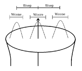
Figure 7: The figure shows a schematic of the core and conal components along the dipolar open field line region in a normal pulsar. The component widths and their separation are estimated from the lower boundary lines for the distribution of widths with period. The emission is assumed to originate at a constant height above the surface for all the emission components.

The analysis of profile component widths reported in this work suggests a deviation from the conventional view that the period dependence of widths is a consequence of the dipolar geometry in pulsars. We have shown that the $P^{-0.5}$ dependence is indeed seen individually in the core components as well as the conal components. However, this dependence is not a result of dipolar geometry if we assume that the components occupy a small area in the open field line region of pulsars. The $P^{-0.5}$ dependence follows from the light cylinder radius associated with the last open field line and hence any component with an edge not along the last open field line will not follow this dependence. The additional estimates of the underlying widths suggest that they are identical in both the core and conal components. This indicates that the emission heights in normal pulsars are similar across the pulsar magnetosphere at any given frequency contrary to previous claims of the core and conal emission having different locations within the magnetosphere (Rankin, 1990, 1993a).

4.2 Period dependence of Profile widths

It is worthwhile to look at the implications of the component widths on the overall profile width and their period dependence. Firstly, it is unlikely that the measured full width at 50% points stretches out to the last open field lines. As we discuss above the $P^{-0.5}$ scaling of overall widths is not likely due to the effect of dipolar geometry. However, to see the effect of the LBL on full profile widths, specially in pulsars with more than one component, is difficult as the LBL is dominated by S_t and S_d classes with single components. As discussed in section 1 a $P^{-0.5}$ dependence is reported for the opening angle $\rho^{\nu}$ corresponding to measured widths for multiple component profiles (M and T classes). We argued that the dependence is an effect of the estimation process of $\rho^{\nu}$ and follows from the period dependence in the core widths. In order to preserve this relation we found that the quantity $F$ defined in eq.(5) should be period independent. Based on our analysis we are now in a position to verify this claim. As shown earlier, the full width at any frequency $\nu$ can be broken down as $W^{\nu}=W_{core}^{\nu}+2nW_{cone}^{\nu}+2n\delta W^{\nu}$, with $n$=1,2 for the inner and outer cone respectively. We have assumed identical widths for all the conal components (which is very likely given the presence of boundary line) as well as all the separation between components (less well constrained due to the absence of a clear boundary). We have now shown that both $W_{core}^{\nu}$ and $W_{cone}^{\nu}$ follow a $P^{-0.5}$ dependence individually and are more or less identical (which we call $W_{comp}^{\nu}$). The final part gives the distance between adjacent components and can be represented as $\delta W^{\nu}=W_{sep}^{\nu}-W_{comp}^{\nu}$, where $W_{sep}^{\nu}$ is the separation between the adjacent peaks of components. Our estimates of $W_{sep}^{\nu}$ in section 3, did not show an explicit period dependence as seen in the components. But boundary values $W_{sep}$ = 2.66° and $W_{comp}$ = 2.25° implies $\delta W$ = 0.41° ; i.e $\delta W\approx 0.18W_{comp}$. Thus the distance between the components form a small fraction of the component widths. Hence, even if $\delta W$ do not show a $P^{-0.5}$ dependence their contribution to the overall width will be small enough. This means that the factor $F$ in eq.(9) can be approximated to be largely period independent.

5 Summary

In this work we have carried out detailed measurements to characterise the widths of the core and conal components separately for a large number of normal pulsars. We have shown that the component widths when distributed with period show the presence of identical lower boundary lines for both the core and conal components which follow a $P^{-0.5}$ dependence. These results firmly establish the core and the conal components to be equivalent within the pulsar profile and eliminate any requirement for two different emission mechanisms for core and conal emission at different heights (Rankin, 1990, 1993a; Melrose, 2017). We have also highlighted that in normal pulsars where the radio emission is supposed to originate at heights of around 500 kilometers from the stellar surface throughout the pulsar profile, the $P^{-0.5}$ dependence of the lower boundary line is a result of the physical mechanism and not an outcome of the dipolar nature of the magnetic field in the emission region. In the absence of further constraints from observations more detailed modeling of the emission processes are required to explain the period dependence of components.

Acknowledgments: We thank the referee for the comments which helped to improve the paper. We thank Mihir Arjunwadkar for discussion on the LBL analysis techniques. We would like to thank staff of Giant Meterwave Radio Telescope and National Center for Radio Astrophysics for providing valuable support in carrying out this project. This work was supported by grants DEC-2012/05/B/ST9/03924, DEC-2013/09/B/ST9/02177 and UMO-2014/13/ B/ST9/00570 of the Polish National Science Centre.

Table 2: THE TABLE SHOWS THE DETAILS OF THE MEASUREMENTS OF WIDTHS IN PULSARS. THE MEASUREMENTS INCLUDE WIDTHS OF COMPONENTS ($W_{50}$) AND SEPARATION BETWEEN ADJACENT COMPONENTS ($W_{SEP}$). THE FIRST COLUMN PRESENTS THE NAME, THE SECOND COLUMN THE PERIOD ($P$). COLUMNS 4-7 GIVE THE MEASUREMENTS AT 333 MHz, WHICH INCLUDE THE NUMBER OF COMPONENTS $N_{c}$, THE TECHNIQUE USED TO ESTIMATE THE COMPONENT (1 - INTEGRATED PROFILE, 2 - AVERAGING SUBPULSES, 3 - AVERAGING PEAKS IN WINDOW) ALONG WITDH ESTIMATION METHOD (a - FULL WIDTH, b - HALF WIDTH, c - FITTING GAUSSIAN). COLUMNS 8-11 THE CORRESPONDING VALUES AT 618 MHz DATA.

			333 MHz				618 MHz
No	PSR	$P$	$N_{c}$	Method	$W_{50}$	$W_{sep}$	$N_{c}$	Method	$W_{50}$	$W_{sep}$
		[s]			[deg]	[deg]			[deg]	[deg]
1	B0031$-$07	0.94	2	3-a/b	11.29$\pm$0.13 12.27$\pm$0.13	17.14$\pm$0.13	2	3-a/b	9.61$\pm$0.13 9.54$\pm$0.13	16.21$\pm$0.13
2	J0134$-$2937	0.14	1	1-a	16.20$\pm$0.60	-	1	1-a	18.80$\pm$0.90	-
3	B0148$-$06	1.46	2	1-a	6.89$\pm$0.09 4.88$\pm$0.09	30.51$\pm$0.09	2	1-a	6.49$\pm$0.09 6.33$\pm$0.09	27.01$\pm$0.09
4	B0149$-$16	0.83	2	1-a,b	3.38$\pm$0.15 5.01$\pm$0.15	5.72$\pm$0.15	2	1-a,b	2.75$\pm$0.15 4.81$\pm$0.15	5.36$\pm$0.15
5	B0203$-$40	0.63	2	1-a,c	3.83$\pm$0.20 3.33$\pm$0.20	6.46$\pm$0.20	1	1-a	4.13$\pm$1.00	-
6	B0301$-$19	1.39	2	1-a	3.20$\pm$0.09 4.41$\pm$0.09	12.69$\pm$0.09	2	1-a	4.75$\pm$0.09 4.71$\pm$0.09	10.27$\pm$0.09
7	B0450$-$18	0.55	4	1/3-a,b,b	4.49$\pm$0.23 6.49$\pm$0.23 - 5.03$\pm$0.23	7.90$\pm$0.23	4	1-b,c,b	4.03$\pm$0.23 8.46$\pm$0.23 - 6.10$\pm$0.23	7.58$\pm$0.23
8	B0523+11	0.35	2	1-a,b	4.00$\pm$0.35 4.79$\pm$0.35	12.24$\pm$0.35	2	1-a,a	7.83$\pm$0.35 6.51$\pm$0.35	11.24$\pm$0.35
9	B0525+21	3.75	2	1-a,a	2.78$\pm$0.03 2.55$\pm$0.03	14.69$\pm$0.03	-	-	-	-
10	B0540+23	0.25	2	1/3-a	8.34$\pm$0.51 -	18.72$\pm$0.51	2	1/3-a	7.40$\pm$0.51 -	10.44$\pm$0.51
11	B0611+22	0.33	1	1-a	6.95$\pm$0.37	-	1	1-a	5.91$\pm$0.38	-
12	B0626+24	0.48	2	1-a,b	5.86$\pm$0.26 6.68$\pm$0.26	8.17$\pm$0.26	2	1-a	6.36$\pm$0.26 -	6.13$\pm$0.26
13	B0628$-$28	1.24	1	1-a	19.00$\pm$0.10	-	1	1-a	18.33$\pm$0.10	-
14	B0656+14	0.38	-	1-a	15.60$\pm$0.30	-	-	1-a	14.30$\pm$0.60	-
15	B0727$-$18	0.51	3	1-a,b	3.17$\pm$0.25 - 7.23$\pm$0.25	-	3	1-a,b	3.38$\pm$0.25 - 6.33$\pm$0.25	-
16	B0736$-$40	0.37	-	-	-	-	3	1-b,b	- 7.99$\pm$0.33 21.5$\pm$0.33	- 17.72$\pm$0.33
17	B0740$-$28	0.17	3	1 -b,b	6.40$\pm$0.75 - 7.35$\pm$0.75	5.74$\pm$0.75	4	1-b,b	5.39$\pm$0.75 - 4.28$\pm$0.75	2.66$\pm$0.75 3.75$\pm$0.75 -
18	B0756$-$15	0.68	2	1-b,b	3.95$\pm$0.18 2.16$\pm$0.19	2.08$\pm$0.18	2	1-b,b	2.68$\pm$0.18 2.15$\pm$0.18	2.01$\pm$0.18
19	B0818$-$13	1.24	2	3-a/b	3.61$\pm$0.10 3.44$\pm$0.10	2.64$\pm$0.10	2	3-a/b	3.60$\pm$0.1 2.45$\pm$0.10	3.07$\pm$0.10
20	B0818$-$41	0.55	-	-	-	-	2	1-b,b	49.94$\pm$ 2.33 50.76$\pm$2.33	72.00$\pm$2.32
21	B0834+06	1.27	2	1-a,b	2.87$\pm$0.10 3.08$\pm$0.10	4.59$\pm$0.10	2	1-a,b	2.86$\pm$0.1 2.83$\pm$0.10	4.93$\pm$0.10
22	B0844$-$35	1.12	4/5	1-b,a,b	6.83$\pm$0.56 - - 5.18$\pm$0.56 4.26$\pm$0.56	- - 6.75$\pm$0.56 5.16$\pm$0.56	4/5	1-b,a,b	5.64$\pm$0.57 - - 4.29$\pm$0.56 2.83$\pm$0.56	- - 5.56$\pm$0.56 4.76$\pm$0.56
23	J0905$-$4536	0.99	-	-	-	-	2	1-a,a	12.87$\pm$1.92 19.25$\pm$1.93	48.54$\pm$1.91
24	J0905$-$5127	0.35	1	1/2-b,b	9.73$\pm$0.36	-	2	1/2-b,b	4.37$\pm$0.36 2.77$\pm$0.36	4.35$\pm$0.36
25	B0906$-$17	0.40	2	1-a	8.05$\pm$0.31 -	9.59$\pm$0.31	2	1-a	8.14$\pm$0.31 -	-
26	B0919+06	0.43	3	1-b,b	- 5.86$\pm$0.29 5.36$\pm$0.29	- 3.29$\pm$0.29	3	1-b,b	- 4.25$\pm$0.29 5.33$\pm$0.29	- 2.21$\pm$0.29
27	B0942$-$13	0.57	2	1/3-b	2.95$\pm$0.22 -	-	2	1/3-b,b	2.41$\pm$0.22 4.11$\pm$0.22	1.24$\pm$0.22
28	B0950+08	0.25	2	1/3-a,a	16.06$\pm$0.50 14.57$\pm$0.50	34.36$\pm$0.50	2	1/3-a,a	13.50$\pm$0.50 11.97$\pm$0.50	33.63$\pm$0.50
29	B0957$-$47	0.67	-	-	-	-	2	1-a,a	18.93$\pm$1.88 10.48$\pm$1.88	45.17$\pm$1.88
30	J1034$-$3224	1.15	5	1-a,b,b,b	- 6.52$\pm$0.11 13.24$\pm$0.11 - 9.16$\pm$0.11 7.49$\pm$0.11	- 13.77$\pm$0.11 - - 7.31$\pm$0.11	6	1-a,a,c,c,b	18.82$\pm$1.09 7.50$\pm$1.09 12.65$\pm$1.09 - 11.81$\pm$1.09 7.1$\pm$1.09	30.84$\pm$1.09 13.88$\pm$1.09 - - 7.71$\pm$1.09
31	B1039$-$19	1.39	-	-	-	-	3	1-a,b,a	2.47$\pm$0.09 6.58$\pm$0.09 5.74$\pm$0.09	2.87$\pm$0.09 8.87$\pm$0.09
32	B1114$-$41	0.94	1	1-a	5.70$\pm$0.20	-	1	1-a	5.30$\pm$0.20	-
33	B1133+16	1.19	2	1-a,a	1.95$\pm$0.11 3.99$\pm$0.11	7.60$\pm$0.11	2	1-a,a	1.62$\pm$0.11 4.22$\pm$0.11	6.11$\pm$0.11
34	B1237+25	1.38	5	1-a,b,a,c,b	1.51$\pm$0.09 1.60$\pm$0.09 2.01$\pm$0.09 2.24$\pm$0.09 1.76$\pm$0.09	2.56$\pm$0.09 4.48$\pm$0.09 2.82$\pm$0.09 2.24$\pm$0.09	5	1-a,b,b,b	1.40$\pm$0.09 1.48$\pm$0.09 3.06$\pm$0.09 - 2.2$\pm$0.09	2.43$\pm$0.09 4.16$\pm$0.09 2.50$\pm$0.09 1.66$\pm$0.09
35	B1254$-$10	0.62	2	1-a,a	2.95$\pm$0.20 3.08$\pm$0.20	10.61$\pm$0.20	2	1-a,a	4.10$\pm$0.21 2.77$\pm$0.20	10.61$\pm$0.20
36	B1322+83	0.67	-	-	-	-	1	1-a	2.23$\pm$0.19	-
37	B1325$-$43	0.53	2	1-b,b	4.59$\pm$0.24 6.31$\pm$0.24	6.81$\pm$0.24	1	1-a	8.83$\pm$0.24	-
38	B1325$-$49	1.48	5	1-b,b,b,a	2.51$\pm$0.09 - 1.90$\pm$0.09 2.44$\pm$0.08 1.37$\pm$0.08	2.45$\pm$0.09 4.54$\pm$0.09 3.71$\pm$0.09 2.15$\pm$0.09	5	1-b,b,b,a	2.33$\pm$0.09 - 1.81$\pm$0.09 2.02$\pm$0.09 1.53$\pm$0.08	2.33$\pm$0.09 3.83$\pm$0.09 3.53$\pm$0.09 2.39$\pm$0.09
39	J1418$-$3921	1.10	-	-	-	-	2	1-b	4.52$\pm$0.57 -	-
40	B1504$-$43	0.29	1	1-a	7.40$\pm$0.80	-	1	1-a	6.20$\pm$0.80	-
41	B1524$-$39	2.42	2	1-a,a	1.89$\pm$0.05 2.96$\pm$0.05	3.00$\pm$0.05	2	1-a,a	2.20$\pm$0.26 3.09$\pm$0.26	2.75$\pm$0.26
42	J1549$-$4848	0.29	1	1-a	6.40$\pm$0.80	-	1	1-a	7.10$\pm$0.80	-
43	B1552$-$31	0.52	2	1-a,a	4.84$\pm$0.24 5.05$\pm$0.24	15.73$\pm$0.24	2	1-a,a	4.63$\pm$0.24 5.46$\pm$0.24	14.7$\pm$0.24
44	J1557$-$4258	0.33	-	-	-	-	3	1-c,a,c	4.17$\pm$0.41 4.33$\pm$0.38 7.12$\pm$0.40	6.99$\pm$0.38 9.69$\pm$0.38
45	B1556$-$44	0.26	3	1/3-b,a	10.76$\pm$0.49 8.04$\pm$0.49 -	13.79$\pm$0.49 6.9$\pm$0.49	2/ 3	1-b,a	6.49$\pm$0.49 8.12$\pm$0.49 -	13.10$\pm$0.49
46	B1558$-$50	0.86	-	-	-	-	2	1-a,b	2.73$\pm$0.14 3.77$\pm$0.14	4.51$\pm$0.14
47	J1603$-$2531	0.28	1	1-a	10.60$\pm$0.80	-	1	1-a	8.80$\pm$0.80	-
48	B1600$-$49	0.33	-	-	-	-	3	1-c,a,c	3.52$\pm$0.39 4.88$\pm$0.38 5.25$\pm$0.42	7.30$\pm$0.39 8.20$\pm$0.38
49	J1625$-$4048	2.36	-	-	-	-	3	1-a,a,a	1.73$\pm$0.05 3.02$\pm$0.05 3.96$\pm$0.06	10.15$\pm$0.05 6.76$\pm$0.05
50	B1634$-$45	0.12	1	-	-	-	1	1-a	16.40$\pm$1.90	-
51	B1642$-$03	0.39	-	-	-	-	3	1/3-a,b	- 3.63$\pm$0.32 5.60$\pm$0.32	5.48$\pm$0.32 8.68$\pm$0.32
52	J1648$-$3256	0.72	1	1-a	5.98$\pm$0.52	-	1	1-a	5.71$\pm$0.52	-
53	J1700$-$3312	1.36	3	1-b,b	4.32$\pm$0.09 - 4.58$\pm$0.10	-	3	1-b,b	2.01$\pm$0.09 - 3.28$\pm$0.09	3.58$\pm$0.09 5.8$\pm$0.09
54	B1700$-$32	1.21	3	1-b,c,b	5.05$\pm$0.10 4.80$\pm$0.10 3.52$\pm$0.10	5.40$\pm$0.10 5.03$\pm$0.10	3	1-b,c,b	4.61$\pm$0.10 5.76$\pm$0.10 2.74$\pm$0.10	4.78$\pm$0.10 4.57$\pm$0.10
55	J1705$-$3423	0.26	-	-	-	-	1	1-a	20.09$\pm$0.49	-
56	B1706$-$16	0.65	1	1-a	5.80$\pm$0.19	-	1	1-a	5.57$\pm$0.19	-
57	B1706$-$44	0.10	1	1-a	42.30$\pm$ 2.20	-	1	1-a	31.90$\pm$ 2.20	-
58	B1717$-$29	0.62	3	3 a/b	4.99$\pm$0.21 4.99$\pm$0.20 4.99$\pm$0.20	6.53$\pm$0.20 10.20$\pm$0.20	3	3-a/b	4.24$\pm$0.20 4.24$\pm$0.20 4.24$\pm$0.20	7.56$\pm$0.20 8.70$\pm$0.20
59	B1718$-$32	0.48	-	-	-	-	2	1-b,b	3.81$\pm$0.26 7.81$\pm$0.26	5.57$\pm$0.26
60	B1719$-$37	0.24	1	1-a	11.85$\pm$1.60	-	1	1-a	7.52$\pm$1.60	-
61	J1727$-$2739	1.29	2	1 a	13.51$\pm$1.50 10.04$\pm$1.47	25.79$\pm$1.46	2	1-a	6.51$\pm$1.47 6.30$\pm$1.77	22.69$\pm$1.46
62	B1727$-$47	0.83	3	1-b,b	2.71$\pm$0.15 - 2.87$\pm$0.15	-	3	1-a,b	2.50$\pm$0.15 - 2.37$\pm$0.15	-
63	B1730$-$22	0.87	4	1-a,c,a	- 5.13$\pm$0.14 6.02$\pm$0.14 11.65$\pm$0.14	- 10.46$\pm$0.14 11.07$\pm$0.14	4	1-a,c,a	- 6.65$\pm$0.29 10.07$\pm$0.29 4.52$\pm$0.29	- 10.05$\pm$0.29 10.67$\pm$0.29
64	B1730$-$37	0.34	-	-	-	-	2	1-a,a	9.16$\pm$1.88 14.95$\pm$1.91	40.88$\pm$1.86
65	B1732$-$07	0.42	3	1-b,a,b	4.31$\pm$0.30 3.83$\pm$0.30 3.63$\pm$0.30	9.71$\pm$0.30 5.06$\pm$0.30	3	1-b,a,b	- 3.69$\pm$0.30 4.37$\pm$0.30	9.28$\pm$0.30 4.86$\pm$0.30
66	B1736$-$29	0.32	-	-	-	-	1	1-a	8.16$\pm$0.40	-
67	B1737+13	0.80	5	1/3-a,c,b,b	2.79$\pm$0.16 4.15$\pm$0.16 3.81$\pm$0.16 - 3.18$\pm$0.16	3.74$\pm$0.16 6.94$\pm$0.16 3.49$\pm$0.16 4.96$\pm$0.16	5	1/3-a,c,b,b	2.89$\pm$0.16 3.94$\pm$0.16 4.84$\pm$0.16 - 3.01$\pm$0.16	3.63$\pm$0.16 5.73$\pm$0.16 - -
68	B1738$-$08	2.04	4	1-b,b	2.72$\pm$0.06 - - 3.48$\pm$0.06	3.55$\pm$0.06 8.24$\pm$0.06 2.60$\pm$0.06	4	1-b,b	3.42$\pm$0.06 - - 2.70$\pm$0.06	3.16$\pm$0.06 6.11$\pm$0.06 3.08$\pm$0.06
69	B1737$-$39	0.51	2	1-b	10.88$\pm$0.24 -	-	2	1-a	6.51$\pm$0.24 -	-
70	B1742$-$30	0.37	4	1-a,a	5.86$\pm$0.35 - 8.29$\pm$0.34 -	-	4	1/2/3-a,b,a	1.71$\pm$0.34 4.28$\pm$0.34 3.46$\pm$0.34 -	10.83$\pm$0.34 3.88$\pm$0.34 11.33$\pm$0.34
71	B1745$-$12	0.39	3	1-b,b,c	3.62$\pm$0.32 6.27$\pm$0.32 9.51$\pm$0.33	4.49$\pm$0.32 10.66$\pm$0.32	3	1-b,b,c	3.28$\pm$0.32 5.77$\pm$0.32 7.14$\pm$0.32	4.27$\pm$0.32 5.85$\pm$0.32
72	J1750$-$3503	0.68	1	1-a	38.30$\pm$0.30	-	1	1-a	34.00$\pm$0.30	-
73	B1747$-$46	0.74	2	1-b,b	3.53$\pm$0.17 4.44$\pm$0.17	4.17$\pm$0.17	2	1-b,b	3.08$\pm$0.17 4.98$\pm$0.17	3.70$\pm$0.17
74	B1749$-$28	0.56	3	1/3-b,b	3.23$\pm$0.22 3.40$\pm$0.22 -	8.03$\pm$0.22	3	1/3-b,b,b	2.71$\pm$0.22 3.10$\pm$0.22 3.17$\pm$0.22	8.74$\pm$0.22 1.10$\pm$0.22
75	B1754$-$24	0.23	-	-	-	-	1	1-a	22.30$\pm$1.00	-
76	B1758$-$03	0.92	1 /3	1-a	- 4.73$\pm$0.14 -	-	3	1-a	- 2.83$\pm$0.14 -	-
77	B1758$-$29	1.08	3	1-a,a,a	3.23$\pm$0.35 5.46$\pm$0.35 3.73$\pm$0.35	9.33$\pm$0.35 8.84$\pm$0.35	3	1-a,a,a	2.71$\pm$0.35 6.70$\pm$0.35 5.78$\pm$0.35	7.86$\pm$0.35 8.59$\pm$0.35
78	B1804$-$08	0.16	3	1-a	- 10.87$\pm$0.77 -	-	3	1-a	- 5.77$\pm$0.77 -	-
79	J1808$-$0813	0.88	1	1-a	14.90$\pm$0.30	-	1	1-a	11.20$\pm$0.30	-
80	B1813$-$26	0.59	2	1-a,a	11.12$\pm$1.06 11.47$\pm$1.06	26.20$\pm$1.06	2	1-a,b	10.99$\pm$1.06 8.23$\pm$1.07	21.70$\pm$1.06
81	B1813$-$36	0.39	3	1/3-a	- 5.82$\pm$0.32 -	5.70$\pm$0.32	-	-	-	-
82	J1817$-$3837	0.38	-	-	-	-	3	1-b	2.57$\pm$0.60 - -	-
83	B1818$-$04	0.60	2	1-b	4.75$\pm$0.21 -	-	1/2	1-a	4.74$\pm$0.21 -	-
84	B1819$-$22	1.87	2	3-b/a	6.13$\pm$0.20 6.66$\pm$0.20	8.60$\pm$0.20	2	3-b /a	4.59$\pm$0.20 4.78$\pm$0.20	7.82$\pm$0.20
85	J1823$-$0154	0.76	2	1-a	- 60$\pm$0.30	-	2	1-b,a	2.80$\pm$0.16 2.31$\pm$0.16	2.56$\pm$0.16
86	B1821+05	0.75	3	1-a,a,b	3.10$\pm$0.17 4.11$\pm$0.17 6.19$\pm$0.17	13.99$\pm$0.17 10.46$\pm$0.17	3	1-a,a	2.88$\pm$0.17 5.48$\pm$0.17 -	13.40$\pm$0.17 7.90$\pm$0.17
87	B1820$-$31	0.28	2	1/3-a	- 6.40$\pm$0.44	4.06$\pm$0.44	2	1/3-a	- 6.50$\pm$0.44	3.74$\pm$0.44
88	B1831$-$04	0.29	5	1-a,a,a,a	16.07$\pm$1.30 - 21.23$\pm$1.30 14.33$\pm$1.30 14.00$\pm$1.30	20.20$\pm$1.30 21.12$\pm$1.30 35.81$\pm$1.30 22.04$\pm$1.30	5	1-b,b,a,a	19.99$\pm$1.30 - 17.24$\pm$1.30 16.51$\pm$1.30 11.74$\pm$1.30	- - 36.73$\pm$1.30 21.12$\pm$1.30
89	J1835$-$1020	0.30	-	-	-	-	1	1-a	10.80$\pm$0.70	-
90	J1835$-$1106	0.17	1	1-a	26.70$\pm$1.30	-	1	1-a	13.30$\pm$1.30	-
91	B1839+09	0.38	2	1/3-a,b	3.97$\pm$0.33 4.61$\pm$0.33	4.31$\pm$0.33	2	1-a	- 6.40$\pm$0.33	-
92	B1839$-$04	1.84	2	1-a,a	45.48$\pm$ 2.08 34.80$\pm$ 2.08	55.16$\pm$0.20	2	1-a,a	18.68$\pm$0.20 10.22$\pm$0.20	53.26$\pm$0.20
93	J1843$-$0000	0.88	-	-	-	-	1	1-a	12.23$\pm$0.14	-
94	B1842+14	0.38	2	1-a	8.24$\pm$0.33	-	1/2	1-a	9.30$\pm$0.33	-
95	B1844$-$04	0.60	-	-	-	-	2	1-b,b	8.44$\pm$0.21 6.41$\pm$0.21	5.48$\pm$0.21
96	B1845$-$01	0.66	-	-	-	-	-	-	-	-
97	J1848$-$1414	0.30	1	1-a	19.03$\pm$ 3.70	-	1	1-a	13.4$\pm$ 3.70	-
98	B1846$-$06	1.45	-	-	-	-	3	1-a	- 3.30$\pm$0.09 -	-
99	J1852$-$2610	0.34	2	1-a,a	5.80$\pm$0.38 6.88$\pm$0.37	19.75$\pm$0.37	2	1-b,a	8.60$\pm$1.16 7.42$\pm$1.16	17.41$\pm$1.16
100	B1857$-$26	0.61	5	1-b,c,a,c,a	6.28$\pm$0.20 11.24$\pm$0.20 6.04$\pm$0.20 5.40$\pm$0.20 3.92$\pm$0.20	10.25$\pm$0.20 8.11$\pm$0.20 8.53$\pm$0.20 6.65$\pm$0.20	5	1-b,c,c,b	9.73$\pm$0.20 - 8.44$\pm$0.20 8.12$\pm$0.20 4.24$\pm$0.20	-
101	J1901$-$0906	1.78	2	1-a,a	2.48$\pm$0.07 1.55$\pm$0.07	9.29$\pm$0.07	2	1-a,a	2.05$\pm$0.07 1.55$\pm$0.07	8.49$\pm$0.07
102	B1907+10	0.28	3	1-a	- 6.19$\pm$0.44 -	-	3	1-c,a	5.48$\pm$0.47 4.80$\pm$0.44 -	9.05$\pm$0.44
103	B1907+03	2.33	3	1-c,a,a	17.07$\pm$0.27 33.93$\pm$0.27 7.43$\pm$0.27	25.45$\pm$0.27 32.11$\pm$0.27	3	1-b,c,a	16.38$\pm$0.27 35.67$\pm$0.27 7.79$\pm$0.27	23.1$\pm$0.27 31.17$\pm$0.27
104	B1911$-$04	0.83	2	1/3-a	- 2.98$\pm$0.15	3.35$\pm$0.15	2	1/3-a	- 3.21$\pm$0.15	3.44$\pm$0.15
105	B1914+09	0.27	2	1-a,b	6.18$\pm$0.46 4.91$\pm$0.47	7.21$\pm$0.46	2	1-a,a	5.42$\pm$0.47 6.63$\pm$0.47	8.2$\pm$0.46
106	B1915+13	0.19	2	1/3-a	5.22$\pm$0.64 -	-	2	1/3-a	4.75$\pm$0.65 -	-
107	B1917+00	1.27	3	1-b,a	3.13$\pm$0.10 2.26$\pm$0.10 -	3.34$\pm$0.10 3.06$\pm$0.10	3	1-b,a,b	2.67$\pm$0.10 1.97$\pm$0.10 2.45$\pm$0.10	3.27$\pm$0.10 3.62$\pm$0.10
108	J1919+0134	1.60	-	-	-	-	2	1-a,a	9.17$\pm$0.24 4.79$\pm$0.24	10.10$\pm$0.23
109	B1918+19	0.82	4	1-b,bc	5.42$\pm$0.46 12.37$\pm$0.46 - 14.21$\pm$0.46	14.24$\pm$0.46	4	1-b,b	5.15$\pm$0.46 14.83$\pm$0.46 - -	11.01$\pm$0.46 - -
110	B1919+21	1.34	-	-	-	-	3/2	1/2/3-b,b	2.29$\pm$0.09 - 3.41$\pm$0.09	-
111	B1929+10	0.23	2	1-a,b	5.32$\pm$0.55 6.18$\pm$0.55	5.09$\pm$0.55	2	1-a,b	5.90$\pm$0.55 4.58$\pm$0.55	3.52$\pm$0.55
112	B1937$-$26	0.40	2	1-a,b	3.38$\pm$0.31 3.50$\pm$0.31	5.05$\pm$0.31	2	1-a,b	2.54$\pm$0.31 2.57$\pm$0.31	5.05$\pm$0.31
113	B1944+17	0.44	3	3-b/a	- 7.89$\pm$0.28 6.37$\pm$0.28	- 11.98$\pm$0.28	3	3-b/a	- 11.55$\pm$0.28 7.88$\pm$0.28	9.51$\pm$0.28 10.85$\pm$0.28
114	B2003$-$08	0.58	5	1-b,b,a,b,b	8.70$\pm$0.65 6.73$\pm$0.65 8.77$\pm$0.65 8.2$\pm$0.65 8.17$\pm$0.65	13.28$\pm$0.65 16.03$\pm$0.65 14.20$\pm$0.65 10.53$\pm$0.65	5	1-b,c,a,c,b	14.72$\pm$0.66 7.16$\pm$0.66 11.54$\pm$0.65 11.19$\pm$0.65 7.14$\pm$0.66	8.24$\pm$0.66 14.20$\pm$0.66 15.11$\pm$0.65 8.24$\pm$0.65
115	B2043$-$04	1.55	3	3-b /a	- 2.45$\pm$0.08 2.12$\pm$0.08	- 2.89$\pm$0.08	3	3-b /a	- 1.80$\pm$0.08 1.49$\pm$0.08	- 2.86$\pm$0.08
116	B2044+15	1.14	-	-	-	-	2	1-c,a	5.70$\pm$0.11 2.69$\pm$0.11	9.17$\pm$0.11
117	B2045$-$16	1.96	3	1-a,b,a	2.17$\pm$0.06 3.86$\pm$0.06 1.81$\pm$0.06	9.06$\pm$0.06 4.50$\pm$0.06	3	1-a,b,a	2.67$\pm$0.06 4.45$\pm$0.06 1.74$\pm$0.06	8.52$\pm$0.06 3.96$\pm$0.06
118	J2144$-$3933	8.51	1	1-a	0.80$\pm$0.06	-	1	1-a	0.76$\pm$0.12	-
119	B2303+30	1.58	2	3-a/b	3.48$\pm$0.08 2.40$\pm$0.08	3.93$\pm$0.08	-	-	-	-
120	B2310+42	0.35	4	1-b,b,b	- 3.89$\pm$0.36 5.88$\pm$0.36 3.71$\pm$0.36	- 5.07$\pm$0.36 5.32$\pm$0.36	-	-	-	-
121	B2315+21	1.44	2	3-a/b	2.18$\pm$0.09 3.36$\pm$0.09	2.24$\pm$0.09	2	3-a	2.05$\pm$0.26 2.54$\pm$0.26	2.39$\pm$0.26
122	B2327$-$20	1.64	3	1-a,a,b	1.44$\pm$0.08 1.86$\pm$0.08 2.64$\pm$0.08	2.70$\pm$0.08 1.84$\pm$0.08	3	1-a,c	1.49$\pm$0.08 2.06$\pm$0.08 -	2.79$\pm$0.08 1.47$\pm$0.08
123	J2346$-$0609	1.18	2	1-a,a	2.24$\pm$0.11 2.85$\pm$0.11	16.48$\pm$0.11	2	1-a,a	2.27$\pm$0.21 3.23$\pm$0.21	14.04$\pm$0.21

Appendix A Quantile Regression

The quantile regression is distinct from the traditional method of least squares. The least square finds the conditional mean function, $E(y|x)$, where $y$ corresponds to the mean value for the data at variable $x$. The quantile regression on the other hand gives a more generalized response function, $Q_{q}(y|x)$, where the quantile $q$ (0 $<q<$ 1) is such that $y$ splits the data at any $x$ with $q$ fraction below $y$ and 1-$q$ fraction above $y$. If the prediction error of a model function is $\epsilon_{i}$ for the $i^{th}$ variable, in least squares the minimization of the term $\sum_{i}\epsilon_{i}^{2}$ is carried out. In quantile regression asymmetric penalties are sought with weights (1-$q$)$|\epsilon_{i}|$ for over prediction and $q|\epsilon_{i}|$ for under prediction.

Let us consider $\hat{y}(x)$ to denote the prediction function and $\epsilon(x)=y-\hat{y}(x)$ to denote the prediction error. Then $E(\epsilon(x))=E(y-\hat{y}(x))$ denotes the loss associated with the prediction error. In the least square formulation the loss function is $E(\epsilon)=\epsilon^{2}$. In quantile regression if $\hat{y}^{q}(x)$ is the $q^{th}$ quantile prediction then the loss associated with the prediction error is asymmetric with either $E_{i}^{q}(y-\hat{y}(x_{i}))=q|y_{i}-\hat{y}(x_{i})|$ if $y_{i}\geq\hat{y}(x_{i})$ or $E_{i}^{q}(y-\hat{y}(x_{i}))=(1-q)|y_{i}-\hat{y}(x_{i})|$ if $y_{i}<\hat{y}(x_{i})$. The objective function for minimization is given as :

$$Q(\hat{y}^{q})=\sum_{y_{i}\geq\hat{y}^{q}(x_{i})}q|y_{i}-\hat{y}^{q}(x_{i})|+\sum_{y_{i}<\hat{y}^{q}(x_{i})}(1-q)|y_{i}-\hat{y}^{q}(x_{i})|$$ (A1)

The above function is non differentiable but can be minimized using the simplex method to find the optimal solution for $\hat{y}^{q}(x)$.

The lower boundary line in the component width distribution with period was estimated using quantile regression. The data was converted to logarithmic scale in order to make the boundary line ($\hat{y}^{q}(x)=ax+b$) a linear function of period. The quantile regression is implemented in the statsmodel Python module’s QuantReg class which was used for these estimates. We investigated the boundary line for multiple definition of the quantile $q$ = 0.05, 0.1, 0.2, 0.3, 0.4, 0.5. The results for each case is shown in figure 8 where all the component widths have been considered. As seen in the figure the boundary line has a slope close to -0.5 for all $q\geq$ 0.1 reproducing the period dependence. Hence, we have used $q$ = 0.1 as our quantile level for estimating the lower boundary line.

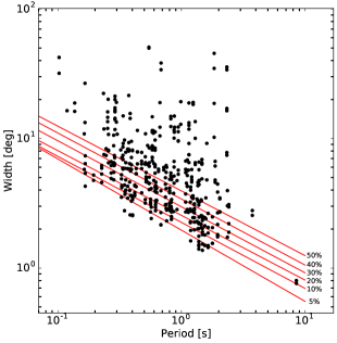
Figure 8: The plot shows the quantile regression analysis for the component widths as a function of the period. The quantile regression is estimated for $q$ = 0.05, 0.1, 0.2, 0.3, 0.4, 0.5. The lower boundary has a period dependence $\sim$ -0.5 for $q\geq$ 0.1, but the dependence is not well constrained for $q$ = 0.05. We have used $q$ = 0.1 as our estimate for the lower boundary which correspond to $W=2.25P^{-0.51}$ in the above case.

References

- Arendt & Eilek (2002) Arendt, P.N.; Eilek, J.A. 2002, ApJ, 581, 451
- Asseo & Melikidze (1998) Asseo, E.; Melikidze, G.I. 1998, MNRAS, 301, 59
- Bai & Spitkovski (2010) Bai, X.N.; Spitkovski, A. 2010, ApJ, 715, 1270
- Basu et al. (2015) Basu, R.; Mitra, D.; Rankin, J.M. 2015, ApJ, 798, 105
- Basu et al. (2016) Basu, R.; Mitra, D.; Melikidze, G.I.; Maciesiak, K.; Skrzypczak, A.; Szary, A. 2016, ApJ, 833, 29
- Basu et al. (2017) Basu, R.; Mitra, D.; Melikidze, G.I. 2017, ApJ, 846, 109
- Beskin et al. (1993) Beskin, V.S.; Gurevich, A.V.; Istomin, Y.N. 1993, Physics of the pulsar magnetosphere, book.
- Blaskiewicz et al. (1991) Blaskiewicz, M.; Cordes, J. M.; Wasserman, I. 1991, ApJ, 370, 643
- Chen & Beloborodov (2014) Chen, A.Y.; Beloborodov, A.M. 2014, ApJ, 795, L22
- Craig & Romani (2012) Craig, H.A.; Romani, R.W. 2012, ApJ, 755, 137
- Clemens & Rosen (2004) Clemens, J.C.; Rosen, R. 2004, ApJ, 609, 340
- Dyks & Harding (2004) Dyks, J.; Harding, A.K. 2004, ApJ, 614, 869
- Dyks (2008) Dyks, J. 2008, MNRAS, 391, 859
- Everett & Weisberg (2001) Everett, J. E., Weisberg, J. M. 2001, ApJ, 553, 341
- Fung et al. (2006) Fung, P.K.; Khechinashvili, D.; Kuijpers J. 2006, A&A, 445, 779
- Gil et al. (1984) Gil, J.A.; Gronkowski P.; Rudnicki W. 1984, A&A, 132, 312
- Hakobyan & Beskin (2014) Hakobyan, H.L.; Beskin, V.S. 2014, ARep, 58, 889
- Hibschman & Arons (2001) Hibschman, J.A.; Arons, J. 2001, ApJ, 546, 382
- Kijak & Gil (1997) Kijak, J.; Gil, J. 1997, MNRAS, 288, 631
- Kijak & Gil (2003) Kijak, J.; Gil, J. 2003, A&A, 397, 969
- Krzeszowski et al. (2009) Krzeszowski, K.; Mitra, D.; Gupta, Y.; Kijak, J.; Gil, J.; Acharyya, A. 2009, MNRAS, 393, 1617
- Kumar & Gangadhara (2012a) Kumar, D.; Gangadhara, R.T. 2012a, ApJ, 746, 157
- Kumar & Gangadhara (2012b) Kumar, D.; Gangadhara, R.T. 2012b, ApJ, 754, 55
- Kumar & Gangadhara (2013) Kumar, D.; Gangadhara, R.T. 2013, ApJ, 769, 104
- Maciesiak et al. (2011a) Maciesiak, K.; Gil, J.; Ribeiro, V.A.R.M. 2011a, MNRAS, 414, 1314
- Maciesiak et al. (2011b) Maciesiak, K.; Gil, J. 2011b, MNRAS, 417, 1444
- Maciesiak et al. (2012) Maciesiak, K.; Gil, J.; Melikidze, G. 2012, MNRAS, 424, 1762
- Melikidze et al. (2000) Melikidze, G.I.; Gil, J.A.; Pataraya, A.D. 2000, ApJ, 544, 1081
- Melikidze et al. (2014) Melikidze, G.I.; Mitra, D.; Gil, J.A. 2014, ApJ, 794, 105
- Melrose (2017) Melrose, D.B. 2017, RvMPP, 1, 5
- Michel (1982) Michel, F.C. 1982, RvMP, 54, 1
- Mitra & Li (2004) Mitra, D.; Li, X.H. 2004, A&A, 421, 215
- Mitra & Seiradakis (2004) Mitra, D.; Seiradakis, J.H. Hellenic Astronomical Society: Proceedings of the Sixth Astronomical Conference, held at Penteli, Athens, 15-17 September, 2003. Edited by Paul Laskarides. Published by the Editing Office of the University of Athens, Athens, Greece, 2004, p.205
- Mitra et al. (2007) Mitra, D.; Rankin, J.M.; Gupta, Y. 2007, MNRAS, 379, 932
- Mitra et al. (2009) Mitra, D.; Gil, J.A.; Melikidze, G.I. 2009, ApJ, 696, L141
- Mitra & Rankin (2011) Mitra, D., Rankin, J.M. 2011, ApJ, 727, 92
- Mitra et al. (2016a) Mitra, D.; Rankin, J.M.; Arjunwadkar, M. 2016a, MNRAS, 460, 3063
- Mitra et al. (2016b) Mitra, D.; Basu, R.; Maciesiak, K.; Skrzypczak, A.; Melikidze, G.I.; Szary, A.; Krzeszowski, K. 2016b, ApJ, 833, 28
- Mitra (2017) Mitra, D. 2017, JApA, 38, 52
- Petrova & Lyubarskii (2000) Petrova, S.A.; Lyubarskii, Y.E. 2000, MNRAS, 355, 1168
- Philippov & Spitkovsky (2014) Philippov, A.A.; Spitkovsky, A. 2014, ApJ, 785, L33
- Philippov et al. (2015) Philippov, A.A.; Spitkovsky, A.; Cerutti, B. 2015, ApJ, 801, L19
- Radhakrishnan & Cooke (1969) Radhakrishnan, V.; Cooke, D.J. 1969, Astrophys. Lett., 3, 225
- Rankin (1990) Rankin, J.M. 1990, ApJ, 352, 247
- Rankin (1993a) Rankin, J.M. 1993a, ApJ, 405, 285
- Rankin (1993b) Rankin, J.M. 1993b, ApJS, 85, 145
- Ruderman & Sutherland (1975) Ruderman, M.A.; Sutherland, P.G. 1975, ApJ, 196, 51
- Smith et al. (2013) Smith, E.; Rankin, J.M.; Mitra, D. 2013, MNRAS, 435, 1984
- Szary et al. (2015) Szary, A., Melikidze, G.I., Gil, J. 2015, MNRAS, 447, 2295
- Timokhin & Arons (2013) Timokhin, A.N.; Arons, J. 2013, MNRAS, 429, 20
- von Hoensbroech & Xilouris (1997) von Hoensbroech, A.; Xilouris, K.M. 1997, A&A, 324, 981
- Weltevrede & Johnston (2008) Weltevrede, P.; Johnston, S. 2008, MNRAS, 391, 1210