⁹Be scattering with microscopic wave functions and the CDCC method

Abstract

We use microscopic ⁹Be wave functions defined in a $\alpha+\alpha+n$ multicluster model to compute ⁹Be+target scattering cross sections. The parameter sets describing ⁹Be are generated in the spirit of the Stochastic Variational Method (SVM), and the optimal solution is obtained by superposing Slater determinants and by diagonalizing the Hamiltonian. The ⁹Be three-body continuum is approximated by square-integral wave functions. The ⁹Be microscopic wave functions are then used in a Continuum Discretized Coupled Channel (CDCC) calculation of ⁹Be+²⁰⁸Pb and of ⁹Be+²⁷Al elastic scattering. Without any parameter fitting, we obtain a fair agreement with experiment. For a heavy target, the influence of ⁹Be breakup is important, while it is weaker for light targets. This result confirms previous non-microscopic CDCC calculations. One of the main advantages of the microscopic CDCC is that it is based on nucleon-target interactions only; there is no adjustable parameter. The present work represents a first step towards more ambitious calculations involving heavier Be isotopes.

I Introduction

Exotic nuclei represent a major interest in current nuclear physics Tanihata et al. (2013). These nuclei, close to the driplines, are characterized by a low binding energy of the last nucleon(s). This property leads to a halo structure, well known since 30 years Tanihata et al. (1985). A halo nucleus is considered as a core surrounded by one or two nucleons. Owing to the low binding energy, the spatial extension of the valence nucleons is large, and the associated radii are much larger than in stable nuclei. Exotic nuclei present further interesting properties such as a change of the magic numbers Ozawa et al. (2000).

Most exotic nuclei have a short lifetime, and can be investigated by reactions only. The recent development of radioactive beam facilities over the world provided many new data, which require more and more sophisticated models. The weak binding energy of the projectile, however, needs a special attention since it strongly affects the various cross sections (elastic scattering, breakup, fusion, etc.). To address this issue, a well known approach is the Continuum Discretized Coupled Channel (CDCC) method Austern et al. (1987) which was originally developed to investigate deuteron scattering Rawitscher (1974).

The CDCC method is based on a structure model for the projectile. The simplest approach is of course a two-body model, where the projectile consists of two structureless clusters. Typical examples are $d=p+n$, ${}^{11}{\rm Be}=^{10}$${\rm Be}+n$ or ${}^{8}{\rm B}=^{7}$${\rm Be}+p$. Many works have been performed within this approach. For some nuclei, however, this two-body description is not adapted, and extensions have been recently developed. The first extension is a three-body model of the projectile, which is necessary for nuclei such as ${}^{6}{\rm He}$ Matsumoto et al. (2004), ${}^{9}{\rm Be}$ Descouvemont et al. (2015a); Casal et al. (2015) or ${}^{11}{\rm Li}$ Cubero et al. (2012). Another development of CDCC involves core excitations which are considered in ${}^{19}{\rm C}$ Lay et al. (2016) and in ${}^{11}{\rm Be}$ de Diego et al. (2017), for example.

The determination of the scattering matrices in the CDCC method makes use of fragment-target optical potentials. This technique provides a set of coupled-channel equations which leads to the projectile-target wave functions and to the scattering matrices. The projectile breakup, important for weakly bound nuclei, is simulated by approximate continuum states of the projectile. These states, also referred to as pseudostates, do not have a physical meaning, but allow to take account of the projectile breakup. For weakly bound nuclei, the cross sections are in general different whether breakup is included or not. As mentioned before, most CDCC calculations are performed within a two-body or a three-body model. A drawback of this approach is that it requires the knowledge of fragment-target optical potentials, which are sometimes poorly known, or not known at all. In these circumstances, simplifying assumptions are necessary.

In a recent development, the projectile is described within a microscopic model, where all nucleons are involved Descouvemont and Hussein (2013); Descouvemont et al. (2015b). The main advantage of this approach is that only nucleon-target optical potentials are needed. These potentials are known over a wide range of energies and masses, and accurate parametrizations are available Varner et al. (1991); Koning and Delaroche (2003). Several variants of microscopic models have been developed. In particular, cluster models Horiuchi et al. (2012) are well adapted to CDCC calculations. In cluster models, the $A$-nucleon structure is taken into account, but the nucleons are assumed to be grouped in clusters Wildermuth and Tang (1977). This approximation permits a simplification of the calculations, whilst it keeps the microscopic character of the model. Besides, the cluster structure is a natural starting point for the treatment of breakup. Recently, ${}^{7}{\rm Li}$ Descouvemont and Hussein (2013) and ${}^{6}{\rm He}$ Descouvemont (2016a) scatterings have been studied within this formalism.

A challenge for cluster models is the description of nuclei involving several clusters. In that case, the number of degrees of freedom is large, and the choice of the basis functions requires a special attention. This problem can be efficiently addressed by using the Stochastic Variational Method (SVM) Kukulin and Krasnopol’sky (1977); Varga and Suzuki (1995). The SVM randomly generates parameter sets of the wave function, and it permits to achieve convergence by superposing several Slater determinants, even when many parameters are involved (see, for example, Ref. Horiuchi and Suzuki (2014)). Our goal for the future is to apply the SVM to nucleus-nucleus reactions, where one of the colliding particles is an exotic light nucleus. In particular, ${}^{11}{\rm Be}$+target reactions provide a strong evidence for a halo structure in ${}^{11}{\rm Be}$ Di Pietro et al. (2012). The traditional description of ${}^{11}{\rm Be}$ is a two-body ${}^{10}{\rm Be}+n$ potential model. However, our aim is to go beyond this simple approximation, and to use a microscopic description of ${}^{11}{\rm Be}$. It has been shown that a multicluster microscopic model based on two $\alpha$ particles and on additional neutrons provides a precise description of low-lying states of Be isotopes Itagaki and Okabe (2000); Itagaki et al. (2000, 2002); Itagaki and Hagino (2002a); Itagaki et al. (2003).

In the present work, we want to explore multicluster wave functions for the projectile description. Our first application deals with ⁹Be, considered as an $\alpha+\alpha+n$ three-cluster system. The microscopic structure calculation is performed using the idea of SVM, and obtained transition densities are utilized in the CDCC calculation. It is known that breakup effects are likely weaker in ${}^{9}{\rm Be}$ and ${}^{10}{\rm Be}$ than in ${}^{11}{\rm Be}$ Di Pietro et al. (2012). However, many data on elastic scattering are available, and ${}^{9}{\rm Be}$ + target scattering is an excellent test before considering more ambitious systems, involving ${}^{10}{\rm Be}$ or ${}^{11}{\rm Be}$. As the model is parameter free, validity tests on well known systems are necessary.

The paper is organized as follows. In Sec. II, we present the microscopic model of ⁹Be, and discuss the main properties (energy spectrum, r.m.s. radii, electric transition probabilities, etc.). Section III is devoted to a brief outline of the microscopic CDCC method. We apply the scattering model to ⁹Be+²⁷Al and ⁹Be+²⁰⁸Pb systems in Sec. IV. These reactions involve a light target, ${}^{27}{\rm Al}$, and an heavy target, ${}^{208}{\rm Pb}$. Concluding remarks and outlook are presented in Sec. V.

II Microscopic description of the ⁹Be structure

In this section, we explain the structure calculation, which is the microscopic description of ⁹Be based on the $\alpha$+$\alpha$+$n$ model. The idea of the SVM is used for the generation of the basis states. Additional information can be found in Refs. Itagaki and Hagino (2002a); Furumoto et al. (2014). From the wave functions we determine the transition densities, which are then used in the CDCC calculations.

II.1 ⁹Be Hamiltonian

In a microscopic approach, the ⁹Be Hamiltonian $H_{0}$ depends on all nucleon coordinates, and is given by

$$H_{0}=\sum_{i=1}^{9}t_{i}-T_{c.m.}+\sum_{i\leq j=1}^{9}v_{ij},$$ (1)

where the center-of-mass kinetic energy $T_{c.m.}$ is subtracted to guarantee the translation-invariance of the wave functions. In this Equation, $t_{i}$ is the kinetic energy of nucleon $i$, and $v_{ij}$ a nucleon-nucleon interaction. The two-body nucleon-nucleon interaction $v_{ij}$ consists of central ($v_{ij}^{\rm central}$), spin-orbit ($v_{ij}^{\rm spin-orbit}$), and Coulomb parts.

For the central interaction, we adopt the Minnesota potential Thompson et al. (1977) which involves the exchange parameter $u$. The standard value is $u=1$, but it can be slightly modified to reproduce important properties of the system. We have used different values for both parities, in order to reproduce the experimental binding energies of the $3/2^{-}$ ground state and of the $1/2^{+}$ first excited state ($-1.57$ MeV and 0.11 MeV, respectively). These constraints provide $u=0.993$ for positive parity, and $u=0.967$ for negative parity. Throughout the text, energies are defined with respect to the $\alpha+\alpha+n$ threshold.

For the spin-orbit part, we adopt a one-Gaussian type interaction

$$v_{ij}^{\rm spin-orbit}=V_{ls}\boldsymbol{L}\cdot\boldsymbol{S}\,\exp\bigl{[}-(\boldsymbol{r}_{i}-\boldsymbol{r}_{j})^{2}/r_{ls}^{2}\bigr{]}/r_{ls}^{5},$$ (2)

where the operator $\boldsymbol{L}$ stands for the relative angular momentum, and where $\boldsymbol{S}$ is the total spin, ($\boldsymbol{S}=\boldsymbol{S}_{1}+\boldsymbol{S}_{2}$). The strength and range, $V_{ls}=-20$ MeV.fm⁵ and $r_{ls}=0.1$ fm, have been tested in many previous cases, and we adopt these values. The Coulomb interaction is treated exactly.

For given spin $j$ and parity $\pi$, Hamiltonian (1) is then diagonalized as

$$H_{0}\,\Phi^{jm\pi}_{k}=E^{j\pi}_{0,k}\,\Phi^{jm\pi}_{k},$$ (3)

where $k$ is the excitation level. In the CDCC framework, negative energies $E^{j\pi}_{0,k}$ correspond to physical states, and positive energies to pseudostates, which can be considered as discrete approximations of the continuum. Different techniques are used to find approximate solutions of (3): the Resonating Group Method Horiuchi (1977), the Antisymmetrized Molecular Dynamics Kanada-En’yo and Horiuchi (2001), the Fermionic Molecular Dynamics Fortune and Sherr (2000) or the Molecular Orbit Model Itagaki and Hagino (2002b) are typical methods.

For the CDCC calculation, we need the transition densities. They are calculated with the wave functions of the static calculation as

$$\rho_{kl}^{j_{1}m_{1},j_{2}m_{2}}(\boldsymbol{r})=\langle\Phi^{j_{1}m_{1}}_{k}|\sum_{i}\bigl{(}\frac{1}{2}\pm t_{iz}\bigr{)}\delta(\boldsymbol{r}-\boldsymbol{r}_{i})|\Phi^{j_{2}m_{2}}_{l}\rangle,$$ (4)

where $i$ runs over protons or neutrons. In this definition, $\boldsymbol{t}_{i}$ is the isposin of nucleon $i$, and the signs ”+” and ”-” correspond to the neutron and proton densities, respectively. In the actual calculation, we write the density in a multipole expansion Kamimura (1981) as

$$\rho_{kl}^{j_{1}m_{1},j_{2}m_{2}}(\boldsymbol{r}) = \sum_{\lambda}\langle j_{2}m_{2}\lambda m_{1}-m_{2}|j_{1}m_{1}\rangle$$ (5)

$$\times\rho^{j_{1},j_{2}}_{kl,\lambda}(r)Y_{\lambda m_{1}-m_{2}}^{*}(\Omega_{r})$$

and calculate the matrix elements of $\rho^{j_{1},j_{2}}_{kl,\lambda}(r)$. For the purpose of applying to reaction calculations, we have to carefully describe the tail regions of the densities. The method to directly calculate the multipole densities can be found in Ref. Baye et al. (1994), and we adopt the same formalism.

II.2 Basis wave functions

A ⁹Be intrinsic wave function $\Psi$ is the antisymmetrized product of single-particle wave functions $\psi_{n}$ as

$$\Psi={\cal A}\{\psi_{1}\psi_{2}\psi_{3}\cdot\cdot\cdot\cdot\psi_{9}\},$$ (6)

where $\psi_{n}$ has a Gaussian shape

$$\psi_{n}(\boldsymbol{r}_{n})=\left(\frac{2\nu}{\pi}\right)^{\frac{3}{4}}\exp\left[-\nu\left(\boldsymbol{r}_{n}-\boldsymbol{R}_{n}\right)^{2}\right]\eta_{n}.$$ (7)

In this definition, $\eta_{n}$ represents the spin-isospin component of the wave function, and $\boldsymbol{R}_{n}$ is a parameter representing the center of a Gaussian function for the $n$-th nucleon. The size parameter $\nu$ is equal to $\nu=1/2b^{2}$ and the oscillator parameter $b$ is chosen as 1.36 fm, a standard value for the $\alpha$ particle.

Based on the generator coordinate method (GCM), the superposition of different wave functions can be done as

$$\Phi^{jm\pi}=\sum_{i=1}^{N}\sum_{K}c_{i}P^{j}_{mK}P^{\pi}\Psi_{i},$$ (8)

where $K$ is the projection of the angular momentum on the intrinsic axis. The states projected on different $K$ quantum numbers are mixed. We superpose $N$ different Slater determinants, and $N$ is 175 in the present model. Here, $\{\Psi_{i}\}$ is a set of Slater determinants with different values {$\boldsymbol{R}_{i}$ }, and the coefficients for the linear combination, $\{c_{i}\}$, are obtained by solving the Hill-Wheeler equation.

The projection on parity and angular momentum is performed by introducing the projection operators $P^{j}_{mK}$ and $P^{\pi}$, and these are carried out numerically. The angular momentum projection is performed using the Wigner function ${\cal D}^{j}_{mK}(\Omega)$ and rotation operator ${\cal R}(\Omega)$,

$$P^{j}_{mK}\Psi_{i}={1\over 8\pi^{2}}\int d\Omega\,{\cal D}^{j*}_{mK}(\Omega)\,{\cal R}(\Omega)\,\Psi_{i},$$ (9)

where ${\cal R}(\Omega)$ rotates both the Gaussian center parameters $\{\boldsymbol{R}_{i}\}$ and the spin part of the wave functions, and $\Omega$ stands for the Euler angles, $\alpha$, $\beta$, and $\gamma$. We have to solve the motion of the valence neutron, which is spatially extended. In these conditions, we need a large number of mesh points for the Euler angles to guarantee the numerical accuracy.

The parity projection is performed by superposing another Slater determinant, where the Gaussian center parameters are spatially inverted,

$$P^{\pi}=(1+P^{r})/\sqrt{2},$$ (10)

where $P^{r}$ is the operator which inverts the spatial coordinates of the Gaussian center parameters, $P^{r}\Psi(\{\boldsymbol{R}_{i}\})$ = $\Psi(\{-\boldsymbol{R}_{i}\})$.

II.3 Generation of the Gaussian center parameters

We superpose different configurations as in Eq. (8). For this purpose, we generate many different sets of the Gaussian center parameters $\{\boldsymbol{R}_{n}\}$ ($n=1,2,3,\ldots,9$) in Eq. (7). We use random numbers to achieve a fast convergence of the energy based on the spirit of the SVM Kukulin and Krasnopol’sky (1977); Varga and Suzuki (1995) and of the antisymmetrized molecular dynamics – superposition of selected snapshots (AMD triple-S) Itagaki et al. (2003).

The two-$\alpha$ cluster parts ($n=1-8$) are introduced with a relative distance $R$,

$$\boldsymbol{R}_{n}=-\frac{R}{2}\boldsymbol{e}_{z}$$ (11)

for $n=1-4$ and

$$\boldsymbol{R}_{n}=+\frac{R}{2}\boldsymbol{e}_{z}$$ (12)

for $n=5-8$, where $\boldsymbol{e}_{z}$ is a unit vector along the $z$ axis. The $R$ values are generated between 0 fm and 5 fm with a uniform distribution.

For the valence neutron ($n=9$), we have to precisely describe the wave function up to the tail region. For the three directions ($k=x,y,z$), the Gaussian center parameter of the valence neutron $(\boldsymbol{R}_{9})_{k}$ is generated using random numbers $\{r_{i}\}$ which are not equally distributed but have the probability proportional to $\exp(-r_{i}/\sigma)$, where $\sigma=4$ fm is introduced. Positive and negative values are generated with equal probability. In this way we generate 175 Slater determinants with different sets of Gaussian center parameters. In the actual calculation, we prepared different sets of Gaussian center parameters using different random numbers and compared the results. The energies of the states, which are candidates for the resonances, are almost the same, and continuum solutions are also very similar.

In the original SVM, the selection of important basis states was performed. On the other hand, here we employ all the basis states generated. The selection of the basis states works well for bound states and for narrow resonances, which are well confined inside the interaction range. However, for continuum states, which are important in the present case, the selection sometimes restricts too much the functional space. If the number of valence nucleons increases, we eventually need a selection of the basis states, but here, we employ all the basis states.

II.4 ⁹Be properties

Figure 1: Energy convergence of the $3/2^{-}$ (a) and $1/2^{+}$ (b) states [$E^{3/2^{-}}_{0,k}$ and $E^{1/2^{+}}_{0,k}$ in Eq. (3)] as a function of number of Slater determinants [$N$ in Eq. (8)]. The dotted lines show the $\alpha$+$\alpha$+$n$ threshold.

The energy convergence of the $3/2^{-}$ and $1/2^{+}$ states is illustrated in Figs. 1 (a) and (b), respectively. Clearly, $N=175$ provides energies close to convergence. The monopole density distributions of the ground state and of the first excited state are shown in Fig. 2. As expected, the neutron density of the $1/2^{+}$ state extends to large distances. This statement is true for most pseudostates. The root mean square matter radius of the ground state is 2.45 fm, in excellent agreement with the experimental value Tanihata et al. (1985) ($2.45\pm 0.01$ fm) and previous works Okabe et al. (1977); Okabe and Abe (1979); Arai et al. (1996). The root mean square matter radius of the first excited state, $1/2^{+}_{1}$, is 3.83 fm.

For the electromagnetic properties, the quadrupole moment $Q$ of the ground $3/2^{-}$ state is calculated as 5.82 $e^{2}$fm², rather close to the experimental value Tilley et al. (2004) ($5.288\pm 0.038$ $e^{2}$fm²). Since the charge distribution is coming only from the two $\alpha$ part, the $E1$ transition from the ground $3/2^{-}$ state to the first $1/2^{+}$ state occurs as a result of recoil effect due to the presence of the valence neutron. Therefore, to properly evaluate the $B(E1)$ value, which is essential in calculating the reaction cross section, solving the neutron wave function up to the long range region is quite important. The present model gives $B(E1)=0.0460\,e^{2}$fm², which is consistent with the observations ($0.027(2)\sim 0.0685\,e^{2}$fm² Burda et al. (2010)). For E2 transitions, the $B(E2)$ value from the ground $3/2^{-}$ state to the $5/2^{-}$ state is 25.8 $e^{2}$fm⁴.

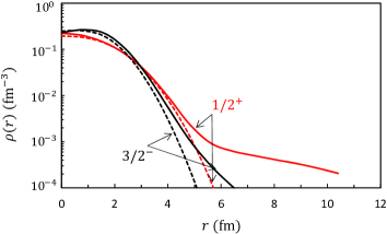
Figure 2: Neutron (solid lines) and proton (dashed lines) monopole densities of the $3/2^{-}$ and $1/2^{+}$ states.

III Microscopic CDCC formalism

In the standard CDCC formalism, the projectile is described by a two-body Rawitscher (1974) or by a three-body Matsumoto et al. (2004) model. The corresponding Hamiltonian is diagonalized over a basis, and the eigenstates are used in an expansion of the projectile-target wave functions. The projectile continuum is simulated by the positive-energy eigenvalues, referred to as pseudostates (PS).

The total Hamiltonian of the projectile + target system is given by

$$H=H_{0}+T_{R}+V_{\rm int},$$ (13)

where $H_{0}$ is the internal Hamiltonian of the projectile, $T_{R}$ is the kinetic energy depending on the relative coordinate $R$, and $V_{\rm int}$ involves optical potentials between the target and the constituents of the projectile. This term depends on the internal coordinates of the projectile, and on the relative coordinate $R$.

The first step of the CDCC method is to diagonalize $H_{0}$ as mentioned in Eq. (3). With the eigenstates $\Phi^{jm\pi}_{k}$ we define the channel wave functions $\varphi^{JM\Pi}_{c}$ as

$$\varphi^{JM\Pi}_{c}=i^{L}\bigl{[}\Phi^{j\pi}_{k}\otimes Y_{L}(\Omega_{R})\bigr{]}^{JM},$$ (14)

where $(J\Pi)$ are the total angular momentum and parity, and where $\Pi=\pi(-1)^{L}$. The total wave function is then expanded as

$$\Psi^{JM\Pi}=\frac{1}{R}\sum_{c}\varphi^{JM\Pi}_{c}\,u^{J\Pi}_{c}(R),$$ (15)

where index $c$ stands for $c=(j,\pi,k,L)$. Expansion (15) assumes a spin zero for the target, but is general regarding the description of the projectile.

After inserting expansion (15) in the Schrödinger equation, the radial functions $u^{J\Pi}_{c}(R)$ are determined from the coupled-channel system

$$\bigl{[}T_{L}+E_{c}-E\bigr{]}u^{J\Pi}_{c}(R)+\sum_{c^{\prime}}V^{J\Pi}_{c,c^{\prime}}(R)u^{J\Pi}_{c^{\prime}}(R)=0,$$ (16)

where the kinetic-energy operator is

$$T_{L}=-\frac{\hbar^{2}}{2\mu_{PT}}\left(\frac{d^{2}}{dR^{2}}-\frac{L(L+1)}{R^{2}}\right),$$ (17)

$\mu_{PT}$ being the reduced mass of the system. In Eq. (16), the coupling potentials are defined by

$$V^{J\Pi}_{c,c^{\prime}}(R)=\langle\varphi^{JM\Pi}_{c}|V_{\rm int}|\varphi^{JM\Pi}_{c^{\prime}}\rangle.$$ (18)

The integration is performed over the internal coordinates of the projectile, and over the relative angle $\Omega_{R}$. Again, Eqs. (16-18) are common to all CDCC approaches. The calculation of the coupling potentials, however, depends on the description of the projectile or, in other words, on the structure of the internal wave functions $\Phi^{jm\pi}_{k}$.

The main specificity of the microscopic CDCC is the interaction potential which reads

$$V_{\rm int}(\boldsymbol{R},\boldsymbol{r}_{i})=\sum_{i=1}^{A_{p}}V_{Ti}(\boldsymbol{R}-\boldsymbol{r}_{i})$$ (19)

where $\boldsymbol{r}_{i}$ are the nucleon coordinates, and $V_{Ti}(\boldsymbol{S})$ is an optical potential between nucleon $i$ and the target. This potential includes the Coulomb interaction, and depends on isospin. The calculation of the coupling potentials (18) is then performed by using a folding technique, which makes use of the projectile densities Descouvemont and Hussein (2013).

Finally, system (16) is solved with the $R$-matrix method Descouvemont and Baye (2010); Descouvemont (2016b) which provides the radial functions, and the corresponding scattering matrices. The cross sections are deduced from the scattering matrices by using standard formula.

IV Application to ⁹Be+²⁷Al and ⁹Be+²⁰⁸Pb scattering

In this section, we apply the model to two systems: ⁹Be+²⁰⁸Pb, typical of heavy targets, and ⁹Be+²⁷Al, typical of light targets. These two collisions have been studied experimentally Woolliscroft et al. (2004); Yu et al. (2010); Gomes et al. (2004), and theoretically in non-microscopic CDCC approaches Descouvemont et al. (2015a); Casal et al. (2015). We cover energies around the Coulomb barrier ($E_{B}\approx 38.9$ MeV for ⁹Be+²⁰⁸Pb, and $E_{B}\approx 8.0$ MeV for ⁹Be+²⁷Al).

In Fig. 3, we show the ⁹Be pseudostate energies for angular momenta $j=1/2,3/2,5/2$. Positive-parity states are indicated by solid lines, and negative-parity states by dashed lines. In addition to the $3/2^{-}$ ground state, the model also reproduces the low-energy $1/2^{+}$ and $5/2^{-}$ resonances. All other states are approximations of the $\alpha+\alpha+n$ continuum, and do not correspond to physical states.

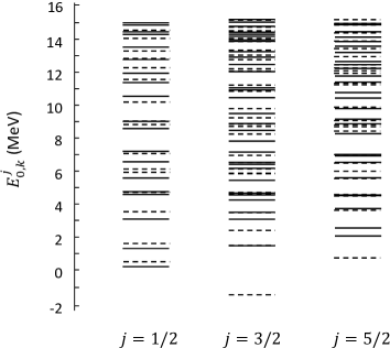
Figure 3: Pseudostate energies for $j=1/2,3/2,5/2$. The solid and dashed lines correspond to the positive and negative parities, respectively.

For the neutron-target optical potential, we take the local potential of Koning and Delaroche Koning and Delaroche (2003) at a neutron energy $E_{n}=E_{\rm lab}/9$. The proton-target interaction only contains the Coulomb term. In all cases, the proton energy $E_{p}=E_{\rm lab}/9$ is much lower than the Coulomb barrier of the $p$+target system, and the corresponding cross sections are purely Rutherford. We take a truncation energy $\mbox{$E_{\rm max}$}=15$ MeV, and a maximum angular momentum of $\mbox{$j_{\rm max}$}=7/2$. Several tests have been done to check the stability of the cross sections against these parameters.

The ⁹Be+²⁰⁸Pb cross sections are presented in Fig. 4, with the data of Refs. Woolliscroft et al. (2004); Gomes et al. (2004). We have selected four typical energies, $E_{\rm lab}=38,44,50$ and 75 MeV. We compare the full CDCC calculation with the single-channel approximation, i.e. by neglecting ⁹Be breakup. At all energies, we have a fair agreement with the data when breakup is included. As found in Refs. Descouvemont et al. (2015a); Casal et al. (2015), the single-channel approximation significantly deviates from the data.

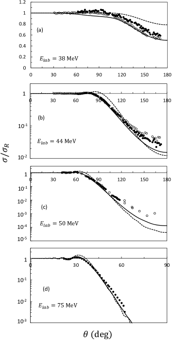
Figure 4: ⁹Be+²⁰⁸Pb elastic cross sections (divided by the Rutherford cross section) at different ⁹Be laboratory energies. Dashed lines: single-channel calculations limited to the ⁹Be ground state; solid lines: full calculations. The experimental data are taken from Ref. Woolliscroft et al. (2004) (filled circles) and Ref. Yu et al. (2010) (open circles).

An example with a light target, ⁹Be+²⁷Al, is shown in Fig. 5. Again, the agreement with the experimental data is quite good, considering that there is no free parameter in the model. For light systems, however, the role of the breakup channels is minor. This was already found in a non-microscopic CDCC analysis Casal et al. (2015).

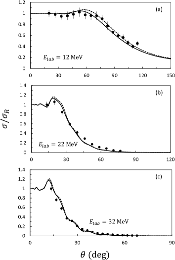
Figure 5: ⁹Be+²⁷Al elastic cross sections (see caption to Fig. 4). The experimental data are taken from Ref. Woolliscroft et al. (2004)

V Conclusion

In this work, we have applied the SVM to ⁹Be wave functions, with the aim of performing CDCC scattering calculations. Elastic scattering is one of the main tools to investigate exotic nuclei, and developing accurate reaction models is a challenge for theory. Owing to their low breakup threshold, exotic nuclei can be easily broken up, and this property must be taken into account in scattering calculations.

The present description of ⁹Be is based on a microscopic multicluster $\alpha+\alpha+n$ model. The wave functions depend on all nucleon coordinates, and are fully antisymmetric. The cluster approximation is used to solve the Schrödinger equation associated with ⁹Be. We use the SVM to optimize the basis functions, where the distances between the $\alpha$ particles, and between their c.m. and the additional neutron are parameters. Optimizing the parameter set is crucial when the number of parameters increases.

We have applied the model to ⁹Be+²⁰⁸Pb and ⁹Be+²⁷Al elastic scattering at various energies around the Coulomb barrier. The only input is the nucleon-target optical potential, which is well known over a wide range of target masses and of nucleon energies. In both cases, we find a fair agreement with the experimental data.

Our goal for the future is to investigate reactions involving heavier Be isotopes, where the number of degrees of freedom in the basis functions is larger. The present application to ⁹Be shows that the method is promising, and that reactions involving ¹⁰Be or ¹¹Be should be feasible in a near future.

References

- Tanihata et al. (2013) I. Tanihata, H. Savajols, and R. Kanungo, Prog. Part. Nucl. Phys. 68, 215 (2013).
- Tanihata et al. (1985) I. Tanihata, H. Hamagaki, O. Hashimoto, Y. Shida, N. Yoshikawa, K. Sugimoto, O. Yamakawa, T. Kobayashi, and N. Takahashi, Phys. Rev. Lett. 55, 2676 (1985).
- Ozawa et al. (2000) A. Ozawa, T. Kobayashi, T. Suzuki, K. Yoshida, and I. Tanihata, Phys. Rev. Lett. 84, 5493 (2000).
- Austern et al. (1987) N. Austern, Y. Iseri, M. Kamimura, M. Kawai, G. Rawitscher, and M. Yahiro, Phys. Rep. 154, 125 (1987).
- Rawitscher (1974) G. H. Rawitscher, Phys. Rev. C 9, 2210 (1974).
- Matsumoto et al. (2004) T. Matsumoto, E. Hiyama, K. Ogata, Y. Iseri, M. Kamimura, S. Chiba, and M. Yahiro, Phys. Rev. C 70, 061601 (2004).
- Descouvemont et al. (2015a) P. Descouvemont, T. Druet, L. F. Canto, and M. S. Hussein, Phys. Rev. C 91, 024606 (2015a).
- Casal et al. (2015) J. Casal, M. Rodríguez-Gallardo, and J. M. Arias, Phys. Rev. C 92, 054611 (2015).
- Cubero et al. (2012) M. Cubero, J. P. Fernández-García, M. Rodríguez-Gallardo, L. Acosta, M. Alcorta, M. A. G. Alvarez, M. J. G. Borge, L. Buchmann, C. A. Diget, H. A. Falou, B. R. Fulton, H. O. U. Fynbo, D. Galaviz, J. Gómez-Camacho, R. Kanungo, J. A. Lay, M. Madurga, I. Martel, A. M. Moro, I. Mukha, T. Nilsson, A. M. Sánchez-Benítez, A. Shotter, O. Tengblad, and P. Walden, Phys. Rev. Lett. 109, 262701 (2012).
- Lay et al. (2016) J. A. Lay, R. de Diego, R. Crespo, A. M. Moro, J. M. Arias, and R. C. Johnson, Phys. Rev. C 94, 021602 (2016).
- de Diego et al. (2017) R. de Diego, R. Crespo, and A. M. Moro, Phys. Rev. C 95, 044611 (2017).
- Descouvemont and Hussein (2013) P. Descouvemont and M. S. Hussein, Phys. Rev. Lett. 111, 082701 (2013).
- Descouvemont et al. (2015b) P. Descouvemont, E. C. Pinilla, and M. S. Hussein, Few-Body Systems 56, 737 (2015b).
- Varner et al. (1991) R. L. Varner, W. J. Thompson, T. L. McAbee, E. J. Ludwig, and T. B. Clegg, Phys. Rep. 201, 57 (1991).
- Koning and Delaroche (2003) A. J. Koning and J. P. Delaroche, Nucl. Phys. A 713, 231 (2003).
- Horiuchi et al. (2012) H. Horiuchi, K. Ikeda, and K. Katō, Prog. Theor. Phys. Suppl. 192, 1 (2012).
- Wildermuth and Tang (1977) K. Wildermuth and Y. C. Tang, A Unified Theory of the Nucleus, edited by K. Wildermuth and P. Kramer (Vieweg, Braunschweig, 1977).
- Descouvemont (2016a) P. Descouvemont, Phys. Rev. C 93, 034616 (2016a).
- Kukulin and Krasnopol’sky (1977) V. I. Kukulin and V. M. Krasnopol’sky, J. Phys. G 3, 795 (1977).
- Varga and Suzuki (1995) K. Varga and Y. Suzuki, Phys. Rev. C 52, 2885 (1995).
- Horiuchi and Suzuki (2014) W. Horiuchi and Y. Suzuki, Phys. Rev. C 89, 011304 (2014).
- Di Pietro et al. (2012) A. Di Pietro, V. Scuderi, A. M. Moro, L. Acosta, F. Amorini, M. J. G. Borge, P. Figuera, M. Fisichella, L. M. Fraile, J. Gomez-Camacho, H. Jeppesen, M. Lattuada, I. Martel, M. Milin, A. Musumarra, M. Papa, M. G. Pellegriti, F. Perez-Bernal, R. Raabe, G. Randisi, F. Rizzo, G. Scalia, O. Tengblad, D. Torresi, A. M. Vidal, D. Voulot, F. Wenander, and M. Zadro, Phys. Rev. C 85, 054607 (2012).
- Itagaki and Okabe (2000) N. Itagaki and S. Okabe, Phys. Rev. C 61, 044306 (2000).
- Itagaki et al. (2000) N. Itagaki, S. Okabe, and K. Ikeda, Phys. Rev. C 62, 034301 (2000).
- Itagaki et al. (2002) N. Itagaki, S. Hirose, T. Otsuka, S. Okabe, and K. Ikeda, Phys. Rev. C 65, 044302 (2002).
- Itagaki and Hagino (2002a) N. Itagaki and K. Hagino, Phys. Rev. C 66, 057301 (2002a).
- Itagaki et al. (2003) N. Itagaki, A. Kobayakawa, and S. Aoyama, Phys. Rev. C 68, 054302 (2003).
- Furumoto et al. (2014) T. Furumoto, T. Suhara, and N. Itagaki, Phys. Rev. C 90, 039902 (2014).
- Thompson et al. (1977) D. Thompson, M. Lemere, and Y. Tang, Nuclear Physics A 286, 53 (1977).
- Horiuchi (1977) H. Horiuchi, Prog. Theor. Phys. Suppl. 62, 90 (1977).
- Kanada-En’yo and Horiuchi (2001) Y. Kanada-En’yo and H. Horiuchi, Progress of Theoretical Physics Supplement 142, 205 (2001).
- Fortune and Sherr (2000) H. T. Fortune and R. Sherr, Phys. Rev. C 61, 024313 (2000).
- Itagaki and Hagino (2002b) N. Itagaki and K. Hagino, Phys. Rev. C 66, 057301 (2002b).
- Kamimura (1981) M. Kamimura, Nucl. Phys. A 351, 456 (1981).
- Baye et al. (1994) D. Baye, P. Descouvemont, and N. K. Timofeyuk, Nucl. Phys. A 577, 624 (1994).
- Okabe et al. (1977) S. Okabe, Y. Abe, and H. Tanaka, Progress of Theoretical Physics 57, 866 (1977).
- Okabe and Abe (1979) S. Okabe and Y. Abe, Progress of Theoretical Physics 61, 1049 (1979).
- Arai et al. (1996) K. Arai, Y. Ogawa, Y. Suzuki, and K. Varga, Phys. Rev. C 54, 132 (1996).
- Tilley et al. (2004) D. R. Tilley, J. H. Kelley, J. L. Godwin, D. J. Millener, J. E. Purcell, C. G. Sheu, and H. R. Weller, Nucl. Phys. A 745, 155 (2004).
- Burda et al. (2010) O. Burda, P. von Neumann-Cosel, A. Richter, C. Forssén, and B. A. Brown, Phys. Rev. C 82, 015808 (2010).
- Descouvemont and Baye (2010) P. Descouvemont and D. Baye, Rep. Prog. Phys. 73, 036301 (2010).
- Descouvemont (2016b) P. Descouvemont, Comput. Phys. Commun. 200, 199 (2016b).
- Woolliscroft et al. (2004) R. J. Woolliscroft, B. R. Fulton, R. L. Cowin, M. Dasgupta, D. J. Hinde, C. R. Morton, and A. C. Berriman, Phys. Rev. C 69, 044612 (2004).
- Yu et al. (2010) N. Yu, H. Q. Zhang, H. M. Jia, S. T. Zhang, M. Ruan, F. Yang, Z. D. Wu, X. X. Xu, and C. L. Bai, J. Phys. G 37, 075108 (2010).
- Gomes et al. (2004) P. R. S. Gomes, R. M. Anjos, C. Muri, J. Lubian, I. Padron, L. C. Chamon, R. L. Neto, N. Added, J. O. Fernández Niello, G. V. Martí, O. A. Capurro, A. J. Pacheco, J. E. Testoni, and D. Abriola, Phys. Rev. C 70, 054605 (2004).