Plank Stars lifetime

Characteristic Time Scales for the Geometry Transition of a Black Hole to a White Hole from Spinfoams

Abstract

Quantum fluctuations of the metric provide a decay mechanism for black holes, through a transition to a white hole geometry. Old perplexing results by Ambrus and Hájíček and more recent results by Barceló, Carballo–Rubio and Garay, indicate a characteristic time scale of this process that scales linearly with the mass of the collapsed object. We compute the characteristic time scales involved in the quantum process using Lorentzian Loop Quantum Gravity amplitudes, corroborating these results but reinterpreting and clarifying their physical meaning. We first review and streamline the classical set up, and distinguish and discuss the different time scales involved. We conclude that the aforementioned results concern a time scale that is different from the lifetime, the latter being the much longer time related to the probability of the process to take place. We recover the exponential scaling of the lifetime in the mass, a result expected from naïve semiclassical arguments for the probability of a tunneling phenomenon to occur.

I Introduction

In his renowned 1974 letter “Black hole explosions?” hawking_black_1974 , Stephen Hawking shows that quantum theory can significantly affect gravity even in low curvature regions, provided that enough time elapses. In the same paper, Hawking closes with the comment that he has neglected quantum fluctuations of the metric and taking these into account “might alter the picture”. Combining these two ideas, Haggard and Rovelli pointed out in haggard_quantum-gravity_2015 that when enough time has elapsed, quantum fluctuations of the metric can spark the geometry transition of a trapped region to an anti–trapped region, and the matter trapped inside the hole can escape. Bouncing black holes scenarios have been extensively considered in the literature, in the context of resolving the central singularity and vis à vis the information loss paradox, see Malafarina:2017csn for a recent review.

The key technical result in haggard_quantum-gravity_2015 is the discovery of a metric describing this process which solves Einstein’s field equations exactly everywhere, except for the compact spacetime transition region. The existence of the exterior metric, which we henceforth refer to as the Haggard–Rovelli (HR) metric, renders this process plausible: General Relativity need only be violated in a compact spacetime region, and this is something that quantum theory allows in general (tunneling). The stability of the exterior spacetime, henceforth called the HR spacetime, after the quantum transition was studied in de_lorenzo_improved_2016 . The known instabilities of white hole spacetimes were shown to possibly limit the duration of the anti–trapped phase, but do not otherwise forbid the transition from taking place.

The physics of the transition region can then be treated à la Feynman, in the spirit of a Wheeler–Misner–Hawking sum–over–geometries misner_feynman_1957 , as sketched in Figure 1. A theory for quantum gravity should be able to predict the probability of this phenomenon to occur and its characteristic time scales. A first attempt to implement this program concretely was given in christodoulou_planck_2016 using the Lorentzian EPRL amplitudes in the context of covariant Loop Quantum Gravity (LQG). Here, we complete the calculation and give an explicit estimate of the relevant time scales.

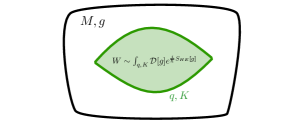
Figure 1: Geometry transition as a path integral over geometries. The shaded region (pale green) is where the quantum transition occurs. Outside this compact spacetime region, quantum theory can be disregarded and the geometry is a solution of Einstein’s equations. This induces an intrinsic metric $q$ and extrinsic curvature $K$ of the boundary surfaces (dark green). The boundary state for the sum over geometries is a semiclassical state, peaked on both $q$ and $K$. The amplitudes of covariant LQG employed here display an emergent behavior as a Wheeler–Misner–Hawking sum in the limit of large quantum numbers.

The assumption of a time symmetric process taken in christodoulou_planck_2016 ; haggard_quantum-gravity_2015 is dropped, allowing also for asymmetric processes as considered in de_lorenzo_improved_2016 . The calculation does not require to specify the boundary surfaces isolating the quantum transition, confirming the assumption in previous works that the scaling estimates are independent of such a choice. We consider the class of spinfoam transition amplitudes defined on 2–complexes that do not have interior faces, which includes the amplitude considered in christodoulou_planck_2016 and roughly corresponds to a tree–level truncation. We do not otherwise specify the 2–complex. Main results from covariant LQG and the spinfoam quantization program are explained briefly with emphasis put on physical intuition. Details on the spinfoam techniques used in this work are given in a companion paper gravTunn , see also mariosPhd .

The paper is organized as follows. Before discussing the black hole case, in Section II we review the simple case of a particle tunneling through a potential wall in non relativistic quantum mechanics. This example allows us to distinguish the different time scales involved in a tunneling process. In Section III we review the HR metric which describes the part of the spacetime well approximated by classical general relativity. We take this opportunity to clarify and streamline some aspects of the HR spacetime. To keep the discussion concise, we present a self–contained construction of the exterior spacetime and explain its main properties, with further properties and details given in the four Appendices B, C, D, E.

In Section IV we explain the construction of the transition amplitude from covariant LQG and the truncation/approximation used. In Section V we estimate characteristic time-scales using Loop Quantum Gravity. These results are confirmed numerically in Appendix A for the explicit choice of boundary, truncation and discretization taken in haggard_quantum-gravity_2015 .

II Tunneling timescales

Consider a particle with energy $E$ that moves towards a potential barrier whose height is $V>E$. Quantum theory predicts that there is a probability $p$ for the particle to cross (“tunnel through”) the potential barrier. Computing $p$ using the time independent Schrödinger equation is a common exercise in introductory quantum mechanics classes. A good approximation to $p$ is given by

$$p\sim e^{-\frac{|S_{E}|}{\hbar}},$$ (1)

which can be arrived at, for instance, using a saddle point approximation for the analytically continued path integral expression for the particle’s propagator. Here, $S_{E}$ is the Euclidean action, which is in general complex, defined as follows. There is no real solution of the classical equation of motion that crosses the barrier, but there is one after analytical continuation to the complex plane. Formally, this amounts to allowing the particle’s velocity to become imaginary. The tunneling suppression exponent corresponds to the imaginary part of the action $S$, evaluated on the complex solution, and we define $S_{E}=i\,S$.

Suppose now that the potential barrier is a square barrier with height $V$, located in the region $0<x<L$. We send a wave packet that at time $T<0$ has a velocity $v>0$ (with mean kinetic energy $E<V$) and is centered at the position $x=v\,T<0$. Around $T=0$ the packet hits the barrier and splits into a reflected packet with an amplitude of modulus squared $1-p$ and a transmitted packet with an amplitude of modulus squared $p$. Suppose there is a detector on the other side of the barrier. The probability of this detector to detect the particle is $p$. But, what is the most probable time $T_{c}$ for the detector to detect the particle? The answer to this question defines the crossing time for a tunneling phenomenon. This is the time the actual tunneling takes to happen.

Next, tunneling is the phenomenon that allows natural nuclear radioactivity. The radioactive decay of a nucleus can be modeled as a quantum particle trapped inside a potential barrier. Imagine we have a wave packet with mean velocity $v$ bouncing back and forth inside a box of size $L$, whose walls are potential barriers of finite hight. The particle will bounce against the wall with a period $\Delta T=L/v$. Thus, $\Delta T$ is a characteristic classical time of the phenomenon and at each bounce the wave packet has a probability $p$ to tunnel. This implies that the probability to exit the barrier per unit time is $P\sim p/\Delta T$. The probability ${P}(T)$ for the particle to exit at time $T$ is then determined by $d{P}(T)/dT=-p\,P(T)$, namely

$${P}(t)=\frac{1}{\tau}\;e^{-\frac{t}{\tau}},$$ (2)

where

$$\tau\sim\frac{1}{P}\sim\frac{\Delta T}{p}$$ (3)

is the lifetime of the nucleus.

We have reviewed these simple physics to point out that there are three distinct time scales at play. [1em]2emLifetime $\tau$: the time it takes a trapped particle to escape a trapping potential barrier.
Crossing time $T_{c}$: the time needed to cross the potential barrier.
Characteristic time $\Delta T$: the time that multiplies the inverse of the tunneling probability to give the lifetime.

The crossing time $T_{c}$ and the lifetime $\tau$ are determined by quantum theory. They can be estimated from the propagator of the particle, contracted with coherent states $\mathinner{|{x,v}\rangle}$ and $\mathinner{|{y,v}\rangle}$ that are peaked on positions $x$ and $y$ left and right of the potential, respectively, and on a momentum given by a constant velocity $v$ and the mass of the particle:

$$W(x,y,v;T)=\langle x,v|e^{-iHT/\hbar}|y,v\rangle,$$ (4)

where $H$ is the Hamiltonian. The crossing time can be estimated as the expectation value

$$T_{c}\sim\frac{\int_{0}^{\infty}dT\ T\ |W(0,L,v;T)|^{2}}{\int_{0}^{\infty}dT\ |W(0,L,v;T)|^{2}},$$ (5)

which determines the average time after which the detector will click, when the tunneling takes place. The probability of the tunneling to take place can be estimated from the amplitude of the propagator at this time

$$p\sim|W(0,L;T_{c})|^{2},$$ (6)

and the lifetime $\tau$ follows from (3). The characteristic time $\Delta T$ is determined by the classical physical scales of the system, and is independent from $\hbar$. All these three time scales have a counterpart in a black to white hole geometry transition.

III Haggard–Rovelli Spacetime

III.1 Global Structure

A HR spacetime haggard_quantum-gravity_2015 ; de_lorenzo_improved_2016 provides a minimalistic model for a geometry where there is a transition of a trapped region (formed by collapsing matter) to an anti–trapped region (from which matter is released). The transition happens via quantum gravitational effects that are non negligible only in a finite spatio–temporal region.

The transition region is excised from spacetime, by introducing a spacelike compact interior boundary, which surrounds the quantum region. Outside this region the metric solves Einstein’s field equations exactly everywhere, including on the interior boundary.

The HR spacetime is constructed by taking the following simplifying assumptions:

• Collapse and expansion of matter are modeled by thin shells of null dust of constant mass $m$.

• Spacetime is spherically symmetric.

These assumptions determine the local form of the metric by virtue of Birkhoff’s theorem, which can be stated as follows HawkEllis : Any solution to Einstein’s equations in a region that is spherically symmetric and empty of matter is locally isomorphic to the Kruskal metric in that region. The HR spacetime is locally but not globally isomorphic to portions of the Kruskal spacetime.

Then, the metric inside the null shells is flat (Schwarzschild with $m=0$), the metric outside the shells is locally Kruskal with $m$ being the mass of the shells and spacetime is asymptotically flat. The trapped and anti–trapped regions are portions of the black and white hole regions of the Kruskal manifold, respectively. In particular, the marginally trapped and anti–trapped surfaces bounding these regions are portions of the $r=2m$ Kruskal hypersurfaces.

The Carter–Penrose diagram of an HR spacetime is given in Figure 2. We are looking to construct a metric such that the surfaces and regions in Figure 2 have the following properties:

• $\mathcal{S}^{-}$ and $\mathcal{S}^{+}$ are null hypersurfaces. The junction condition on the intrinsic metric holds. Their interpretation as thin shells of null dust of mass $m$ follows: The allowed discontinuity in their extrinsic curvature results in a distributional contribution in $T_{\mu\nu}$ on $\mathcal{S}^{-}$ and $\mathcal{S}^{+}$, see next section. This is standard procedure in Vaidya null shell collapse models vaidya_gravitational_1951 , see for instance poisson2004relativist . $T_{\mu\nu}$ vanishes everywhere else in the spacetime.

• The surfaces $\mathcal{F^{+}}$, $\mathcal{F^{-}}$, $\mathcal{C^{+}}$, $\mathcal{C^{-}}$ depicted in Figure 2 are spacelike. Their union $\mathcal{B}\equiv\mathcal{F}^{-}\cup\mathcal{C}^{-}\cup\mathcal{C}^{+}\cup\mathcal{F}^{+}$ constitutes the interior boundary $\mathcal{B}$. The intrinsic metric is matched on the spheres $\Delta$ and $\varepsilon^{\pm}$. The extrinsic curvature is discontinuous on $\varepsilon^{\pm}$, see previous point, and is also discontinuous on $\Delta$ because of the requirement that $C^{\pm}$ are spacelike: the normal to the surface jumps from being future oriented to being past oriented.

• $\mathcal{Z}$ is a spacelike surface. The junction conditions for both the intrinsic metric and extrinsic curvature, hold, including on the sphere $\Delta$. As we will see below, $\mathcal{Z}$ plays only an auxiliary role and need not be further specified, see also Appendix C for this point.

• $\mathcal{M^{-}}$ and $\mathcal{M^{+}}$ are marginally trapped (anti–trapped) surfaces and the shaded regions are trapped (anti–trapped). That is, the expansion of outgoing (ingoing) null geodesics vanishes on $\mathcal{M^{-}}$ ($\mathcal{M^{+}}$), is negative inside the shaded regions and positive everywhere else in the spacetime.

Before explicitly giving the metric, let us comment on the necessity of extending the interior boundary outside the (anti–)trapped regions. By Birkhoff’s theorem and as noted above, the marginally trapped and anti–trapped surfaces $\mathcal{M^{-}}$ and $\mathcal{M^{+}}$ can only be realized as being portions of the $r=2m$ surfaces of the Kruskal spacetime. If these do not meet the interior boundary, they must run all the way to null infinity. Thus, in order to have a consistent physical picture of the spacetime far from the transition, we must allow for non negligible quantum gravitational effects taking place in the vicinity, and crucially, outside, the (anti–)trapped surfaces.

The metric, energy–momentum tensor and expansions of null geodesics are given in Eddington–Finkelstein coordinates in the following section. The metric is given in Kruskal coordinates in Appendix E and the relation of the construction presented here to the original construction in haggard_quantum-gravity_2015 is explained in Appendix C.

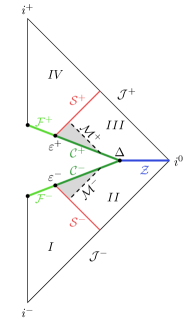
Figure 2: The Haggard–Rovelli spacetime. The collapsing null shell $S^{-}$ emerges as an anti-collapsing null shell $S^{+}$ after a quantum geometry transition. The shaded regions are (anti–) trapped. See Sec.​ III.1 for a detailed description.

III.2 HR metric

In this section we explicitly construct the HR metric in Eddington–Finkelstein (EF) coordinates, in which it takes a particularly simple form. The union of the regions $I$ and $II$ of Figure 2 is coordinatized by ingoing EF coordinates $(v,r)$ and the union of the regions $III$ and $IV$ by outgoing EF coordinates $(u,r)$. There is only the junction condition on $\mathcal{Z}$ to be considered, which we give below. The radial coordinate $r$ will be trivially identified in the two coordinate systems. We work in geometrical units ($G=c=1$).

For the regions $I$ and $II$ the metric reads

$$\mathrm{d}s^{2}=-\left(1-\frac{2m}{r}\Theta(v-v_{\mathcal{S}^{-}})\right)\mathrm{d}v^{2}+2\mathrm{d}v\,\mathrm{d}r+r^{2}\mathrm{d}\Omega^{2},$$

and for the regions $III$ and $IV$

$$\mathrm{d}s^{2}=-\left(1-\frac{2m}{r}\Theta(u-u_{\mathcal{S}^{+}})\right)\mathrm{d}u^{2}-2\mathrm{d}u\,\mathrm{d}r+r^{2}\mathrm{d}\Omega^{2},$$

where $\Theta$ is the Heaviside step function. The ingoing and outgoing EF times $v_{\mathcal{S}^{-}}$ and $u_{\mathcal{S}^{+}}$ denote the position of the shells $\mathcal{S^{-}}$ and $\mathcal{S^{+}}$ in these coordinates.

The two junction conditions on $\mathcal{Z}$ are satisfied by the identification of the radial coordinate along $\mathcal{Z}$ and the condition

$$v-u\stackrel{{\scriptstyle\mathcal{Z}}}{{=}}2r^{\star}(r),\\$$ (9)

where $r^{\star}(r)=r+2m\log{\left|\frac{r}{2m}-1\right|}$. Notice that this relation is the usual coordinate transformation between $(v,r)$ and $(u,r)$. We recall that the EF times are defined as $v=t+r^{\star}(r)$ and $u=t-r^{\star}(r)$, where $t$ is the Schwarzschild time.

We emphasize that we need not and will not choose the hypersurface $\mathcal{Z}$ explicitly. The HR metric is independent of any such choice. The reason it is necessary to consider it formally as an auxiliary structure is that there does not exist a bijective mapping of the union of regions $II$ and $III$ of the HR spacetime to a portion of the Kruskal manifold. That is, it is necessary to use at least two separate charts describing a Schwarzschild line element, as we did above. Where we take the separation of these charts to be (in other words, the choice of $\mathcal{Z}$), is irrelevant. See also Appendix C for this point, in particular Figure 9 and its description.

To explicitly define the metric we need to give the range of the coordinates. Assume an explicit choice of boundary surfaces $\mathcal{B}$ has been given. Having covered every region of the spacetime by a coordinate chart, we can describe embedded surfaces. Since all surfaces $\Sigma$ appearing in Figure 2 are spherically symmetric, it suffices to represent the surfaces as curves in the $v-r$ and $u-r$ planes. Using a slight abuse of notation we write $v=\Sigma(r)$ or, in parametric form, $(\Sigma(r),r)$. The range of coordinates is given by the following conditions. For the regions $I$ and $II$ we have

$$v\in(-\infty,+\infty)\,,\ \ \ r\in(0,+\infty)\,$$

$$v\leq\mathcal{F^{-}}(r)\,,\ \ \ v\leq\mathcal{C^{-}}(r)\,,\ \ \ v\leq\mathcal{Z}(r)\,,$$ (10)

and for the regions $III$ and $IV$ the coordinates satisfy

$$u\in(-\infty,+\infty)\,,\ \ \ r\in(0,+\infty)\,$$

$$u\geq\mathcal{F^{+}}(r)\,,\ \ \ u\geq\mathcal{C^{+}}(r)\,,\ \ \ u\geq\mathcal{Z}(r).$$ (11)

What remains is to ensure the presence of trapped and anti–trapped regions, as in the Carter–Penrose diagram of Figure 2. This is equivalent to the geometrical requirement that the spheres $\varepsilon^{\pm}$ have proper area less than $4\pi(2m)^{2}$ while the sphere $\Delta$ has proper area larger than $4\pi(2m)^{2}$. We may write this in terms of the radial coordinate as

$$r_{\varepsilon^{\pm}} < 2m,$$

$$r_{\Delta} > 2m.$$ (12)

Apart from this requirement, the areas of the spheres $\epsilon^{\pm}$ and $\Delta$ are left arbitrary. Since $\varepsilon^{\pm}$ and $\Delta$ are specified once the boundary is explicitly chosen, this is a condition on the allowed boundary surfaces that can be used as an interior boundary of a HR spacetime: $\mathcal{C^{\pm}}$ can be any spacelike surfaces that have their endpoints at a radius less and greater than $2m$, intersecting in the latter endpoint. Since $\mathcal{C}^{\pm}$ are spacelike, it follows that we necessarily have a portion of the (lightlike) $r=2m$ surfaces in the spacetime along with trapped and anti–trapped regions. See also Figure 10 for this point. The conditions

$$v_{\Delta} \geq v_{\mathcal{S}^{-}},$$

$$u_{\Delta} \leq u_{\mathcal{S}^{+}},$$ (13)

for the coordinates of the sphere $\Delta$ follow from equation (III.2) and the fact that $\mathcal{C}^{\pm}$ are taken spacelike.

The HR spacetime is a two–parameter family of spacetimes, in the following sense. The geometry of the spacetime, up to the choice of the interior boundary $\mathcal{B}$, is determined once two dimension–full, coordinate independent quantities are specified. One parameter is the mass $m$ of the null shells $\mathcal{S}^{\pm}$. The second parameter is the bounce time $T$, the meaning of which is discussed in the following section. We can express $T$ in terms of $u_{\mathcal{S}^{+}}$ and $v_{\mathcal{S}^{-}}$ simply by

$$T=u_{\mathcal{S}^{+}}-v_{\mathcal{S}^{-}}.$$ (14)

As with the mass $m$, the bounce time $T$ is taken to be positive. Details on the positivity of $T$ are given in Appendix D.

Then, the Haggard–Rovelli geometry has two characteristic physical scales: a length scale $Gm/c^{2}$ and a time scale $GT/c^{3}$, where we momentarily reinstated the gravitational constant $G$ and the speed of light $c$. The aim of this article is to compute the probabilistic correlation between the two scales $T$ and $m$ from quantum theory. This will be done in terms of a path integral in the region bounded by the interior boundary $\mathcal{B}$, with the boundary states peaked on the geometry of $\mathcal{B}$, without actually making an explicit choice for the hypersurfaces $\mathcal{C}^{\pm}$ and $\mathcal{F}^{\pm}$ that constitute the boundary $\mathcal{B}$.

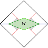
Figure 3: A cross–section of the rotated Carter–Penrose diagram of the HR spacetime, for easier comparison with Figure 1. The amplitude $W(m,T)$ gives the probability for the spacetime with mass $m$ and bounce time $T$ to be realized.

The role of the bounce time $T$ as the second spacetime parameter is obscure in the line elements (III.2) and (III.2). In equation (14), we expressed the bounce time in terms of the coordinate description of the collapsing and expanding (i.e.​ anti–collapsing) shells. The bounce time $T$ is then encoded implicitly in the line element via the Heaviside functions, which imply the inequalities $v\geq v_{\mathcal{S}^{-}}$ and $u\leq u_{\mathcal{S}^{+}}$ that specify the curved part of the spacetime.

We may make $T$ appear explicitly as a dimensionfull parameter in the metric components. This is achieved by shifting both coordinates $u$ and $v$ by

$$v\rightarrow v-\frac{v_{\mathcal{S}^{-}}+u_{\mathcal{S}^{+}}}{2},$$

$$u\rightarrow u-\frac{v_{\mathcal{S}^{-}}+u_{\mathcal{S}^{+}}}{2}.$$ (15)

This is an isometry, since $(\partial_{v})^{\alpha}$ and $(\partial_{u})^{\alpha}$ are the timelike (piecewise, see next section) Killing fields in each region. It simply amounts to shifting simultaneously the origin of the two coordinates systems. The line elements (III.2) and (14) now read

$$\mathrm{d}s^{2}=-\left(1-\frac{2m}{r}\,\Theta\left(v+\frac{T}{2}\right)\,\right)\mathrm{d}v^{2}+2\mathrm{d}v\,\mathrm{d}r+r^{2}\mathrm{d}\Omega^{2},$$

and

$$\mathrm{d}s^{2}=-\left(1-\frac{2m}{r}\,\Theta\left(u-\frac{T}{2}\right)\,\right)\mathrm{d}u^{2}-2\mathrm{d}v\,\mathrm{d}r+r^{2}\mathrm{d}\Omega^{2}.$$

The role of $T$ as a spacetime parameter is manifest in the above form of the metric. It is instructive to compare it with the Vaidya metric for a null shell collapse model, describing the formation of an eternal black hole by a null shell $\mathcal{S}^{-}$ collapsing from past null infinity $\cal{J}^{-}$. Setting the shell to be at $v=v_{\mathcal{S}^{-}}$, the line element would be identical to (III.2), with the difference that the range of the coordinates $(v,r)$ is not constrained by the presence of the surfaces $\mathcal{F^{-}}$, $\mathcal{C^{-}}$ and $\mathcal{Z}$, as in equation (III.2). The choice $v=v_{\mathcal{S}^{-}}$ for the position of the null shell is immaterial in this case and we can always remove $v_{\mathcal{S}^{-}}$ from the line element by shifting the origin as $v\rightarrow v-v_{\mathcal{S}^{-}}$. In the HR metric, the two coordinate charts are related by the junction condition (9). It is impossible to make both $v_{\mathcal{S}^{-}}$ and $u_{\mathcal{S}^{+}}$ disappear from the line element by shifting the origins of the coordinate charts, the best we can do is remove one of the two or, as we did above, a combination of them. This observation emphasizes that the bounce time $T$ is a free parameter of the spacetime. Notice that the junction condition (9) is unaffected by a simultaneous shifting of the form (III.2).

The field equations are solved for the energy momentum tensor blau ; poisson2004relativist

I $\cup$ II :	$T_{\mu\nu}=+\frac{\delta(v+\frac{T}{2})}{4\pi r^{2}}\delta^{v}_{\mu}\delta^{v}_{\nu}$,
III $\cup$ IV :	$T_{\mu\nu}=-\frac{\delta(u-\frac{T}{2})}{4\pi r^{2}}\delta^{u}_{\mu}\delta^{u}_{\nu}$.

The expansion $\theta^{-}$ of outgoing null geodesics in the patch $I$ $\cup$ $II$ and the expansion $\theta^{+}$ of ingoing null geodesics in the patch $III$ $\cup$ $IV$ read

I $\cup$ II :	$\theta^{-}\equiv\nabla_{\mu}k_{-}^{\mu}=\Gamma^{-}\left(1-\frac{2m}{r}\Theta(v+\frac{T}{2})\right)$,
III $\cup$ IV :	$\theta^{+}\equiv\nabla_{\mu}k_{+}^{\mu}=-\Gamma^{+}\left(1-\frac{2m}{r}\Theta(u-\frac{T}{2})\right)$,

where $k_{-}^{\mu}$ and $k_{+}^{\mu}$ are affinely parametrized tangent vectors of the null geodesics and $\Gamma^{\pm}$ are positive scalar functions which we will not need here, see blau ; poisson2004relativist for details. From these expressions, it follows that the spacetime possesses a trapped and an anti–trapped surface, defined as the locus where the expansions $\theta^{-}$ and $\theta^{+}$ vanish respectively, and which we identify with $\mathcal{M^{-}}$ and $\mathcal{M^{+}}$ in Figure 2. Thus, in EF coordinates, $\mathcal{M^{\pm}}$ are given by

$\mathcal{M^{-}}$ :	$r=2m$	, $v\in\left(-\frac{T}{2},\,\mathcal{C^{-}}(2m)\right)$,
$\mathcal{M^{+}}$ :	$r=2m$	, $u\in\left(\mathcal{C^{+}}(2m),\,\frac{T}{2}\right)$.

As explained above, by the requirement $r_{\varepsilon^{\pm}}<2m$ and $r_{\Delta}>2m$, it will always be the case that the surfaces $\mathcal{M^{\pm}}$ are present in the spacetime, along with trapped and anti–trapped regions where $\theta^{\pm}$ are negative. We may explicitly describe the trapped region as the intersection of the conditions $r<2m$, $v\in(-T/2,\mathcal{C^{-}}(2m))$, and $v\leq\mathcal{C^{-}}(r)$. Similarly, the anti–trapped region is given by $r<2m$, $u\in\left(\mathcal{C^{+}}(2m),T/2\right)$ and $u\geq\mathcal{C^{+}}(r)$. The expansions $\theta^{\pm}$ are positive in the remaining spacetime.

III.3 Bounce Time $T$

The bounce time $T$ is a time scale that characterizes the geometry of the HR spacetime. Intuitively, $T$ controls the time separation between the two shells. In this section we discuss the meaning of $T$ as a spacetime parameter.

In equation (14), we expressed the bounce time in terms of the null coordinates labelling the collapsing and expanding shells. As explained in haggard_quantum-gravity_2015 , the bounce time $T$ has a clear operational meaning in terms of the proper time along the worldline of a stationary observer. That is, of an observer at a constant radius $R$, measuring the proper time $\tau_{R}$ between the events at which the worldline intersects the collapsing and expanding shells $S^{\pm}$. A straightforward calculation yields

$$\tau_{R}=\sqrt{f(R)}\,\big{(}\,u_{\mathcal{S}^{+}}-v_{\mathcal{S}^{-}}+2r^{\star}(R)\,\big{)},$$ (18)

where $f(R)=1-\frac{2m}{R}$. Note that to get this expression we must add the contributions from the two line elements (III.2) and (III.2), and use the junction condition (9). Using equation (14), we have

$$T=\frac{\tau_{R}}{\sqrt{f(R)}}-2r^{\star}(R).$$ (19)

Thus, the bounce time $T$ may be measured by an observer, provided she has knowledge of the mass $m$ and of her (coordinate) distance $R$ from the hole.

The physical meaning of $T$ given in haggard_quantum-gravity_2015 is the following. For $R\gg m$, we have

$$T\approx\tau_{R}-2R+\mathcal{O}\left(m\log\frac{R}{m}\right).$$ (20)

Thus, for a far–away inertial observer and to the leading order in $R$, the bounce time $T$ corresponds to the “delay” in detecting the expanding null shell, compared to the time $2R$ it would take for it to bounce back if it were propagating in flat space and was reflected at $r=0$. To be clear, we introduce the dimensionless number $\tilde{R}\equiv R/m$ and bring back $c$ and $G$. The bounce time $T$ can be measured through

$$T\approx\tau_{R}-2\tilde{R}\,\frac{Gm}{c^{2}}+\mathcal{O}\left(\frac{Gm}{c^{2}}\log\tilde{R}\right),$$ (21)

which is a good approximation as long as $\tilde{R}\gg 1$.

Let us now rephrase equation (19) to emphasize the role of $T$ as a spacetime parameter, a coordinate and observer independent quantity, and its relation with the symmetries of the spacetime. The exterior spacetime described by the HR metric has the three Killing fields of a static spherically symmetric spacetime, a timelike Killing field generating time translation and two spacelike Killing fields that together generate spheres. To be precise, these are piecewise Killing fields defined in each of the four regions of Figure 2. Strictly speaking, the spacetime is dynamical, not static, because of the presence of the distributional null shells $S^{\pm}$. The orbits $\Upsilon$ of the timelike Killing field are labelled by an area $A_{\Upsilon}$: The proper area of a sphere generated by the two spacelike Killing fields on any point on $\Upsilon$. This is of course the geometrical meaning of the coordinate $r$.

We can thus avoid to mention any coordinates or observers and specify $T$ through the following geometrical construction. Consider any orbit $\Upsilon$ that does not intersect with the interior boundary surfaces $\mathcal{B}$. The proper time $\tau_{\Upsilon}$ is an invariant integral evaluated on the portion of $\Upsilon$ that lies between its intersections with the null hypersurfaces $S^{\pm}$. For any such $\Upsilon$, we have

$$T=\frac{\tau_{\Upsilon}}{\sqrt{f(A_{\Upsilon})}}-r^{\star}(A_{\Upsilon}).$$ (22)

The bounce time $T$ is independent of the chosen orbit $\Upsilon$ and it is expressed only in terms of invariant quantities – a proper area and a proper time. This expression can be taken to be the definition of $T$.

The bounce time $T$ can be understood in a couple more ways. The radius $r_{\delta}$ defined by $T=2r^{\star}(r_{\delta})$ is where the null shells cross when the HR spacetime is mapped on the Kruskal manifold, as was done in haggard_quantum-gravity_2015 . This construction is explained in Appendix C. The bounce time $T$ can also be understood as a time interval at null infinity, in analogy to an evaporation time, and is also related to the duration of the trapped and anti–trapped phases introduced in bianchi_entanglement_2014 ; de_lorenzo_improved_2016 . These alternatives are discussed in Appendix D.

Geometrical invariants such as areas and angles, will scale both with $m$ and $T$ in the HR spacetime. An interesting property of the HR spacetime is that the (anti–) trapped surfaces $\mathcal{C}^{\pm}$ can be equivalently characterized as the locus where boost angles do not scale with either $m$ or $T$. This is shown in Appendix B, where we also discuss the scaling of other geometrical invariants. We will see in Section IV.4 that the scaling of boost angles with $m$ and $T$ encodes the presence of the (anti–) trapped surfaces $\mathcal{C}^{\pm}$ in the semiclassical boundary state.

 

In summary, the HR spacetime provides a prototypical setup for geometry transition. The geometry of the spacetime depends on two classical physical scales, which become encoded in the geometry of the interior boundary – the boundary condition for the path integral. In turn, quantum theory correlates the two scales in a probabilistic manner.

IV The transition amplitude $W(m,T)$

Since the external geometry of the HR spacetime depends on the two parameters $m$ and $T$, so does the transition amplitude $W(m,T)$ associated to the quantum region. This happens as follows. The HR geometry induces an intrinsic geometry $q_{m,T}$ and an extrinsic geometry $K_{m,T}$ on the boundary $\mathcal{B}$. These depend on $m$ and $T$ since the full metric does. Let $\Psi_{m,T}\equiv\Psi[q_{m,T},K_{m,T}]$ be a coherent semiclassical state peaked on this 3d boundary geometry. Then,

$$W(m,T)=\langle W|\Psi_{m,T}\rangle$$ (23)

is the amplitude for the geometry transition where $\langle W|$ denotes the spinfoam amplitude, discussed below. We invite the reader to compare Figure 3 with Figures 1 and 2 for this point.

We recall that quantum gravity states cannot in general be split into an “in” and “out” state. This is the case here: The intrinsic and extrinsic geometry at the sphere $\Delta$ belongs to both surfaces $\mathcal{C}^{-}$ and $\mathcal{C}^{+}$. Since the state $|\Psi_{m,T}\rangle$ is peaked on the geometry of the entire boundary $\mathcal{B}$, it cannot be decomposed as $|\Psi_{m,T}\rangle\propto|\Psi^{\mathcal{C^{-}}}_{m,T}\rangle\otimes|\Psi^{\mathcal{C^{+}}}_{m,T}\rangle^{\dagger}$. The amplitude is contracted instead with a single boundary state, as suggested by Oeckl’s general boundary formalism oeckl_general_2003 ; oeckl_general_2005 which underpins the covariant approach to LQG.

Formally, the transition amplitude can be written as the contraction of a path integral over 4d geometries for a given boundary 3d geometry, contracted with the semiclassical state peaked on both the intrinsic and extrinsic geometry of the boundary, see Figure 1. Concretely, covariant Loop Quantum Gravity provides explicit formulas for the spinfoam amplitude $\langle W|$ and for coherent states $|\Psi_{m,T}\rangle$. These will be given below. Before that, let us discuss the relation between $W(m,T)$ and the timescales of the quantum transition.

IV.1 Timescales

Our aim is to consider a given black hole formed by collapse and estimate the characteristic time scales suggested by quantum theory. That is, we fix the mass $m$ and study how the quantum theory correlates the mass with the bounce time $T$, which is left arbitrary. Since the classical equations of motion are violated in the transition region, the transition can be viewed as a tunneling phenomenon. As such, it is going to be characterized by the different time scales discussed in Section II.

The analog of the characteristic time of the phenomenon is here simply the mass $\Delta T=m$ (in geometrical units, $G=c=1$). Since the mass $m$ is the only fixed physical scale in our problem and because $\Delta T$ is a classical quantity which cannot depend on $\hbar$, this is the only possible choice for the time scale $\Delta T$. It corresponds to the order of magnitude of the “available time” in the interior of the hole: We recall that the proper time along in–falling timelike trajectories, calculated from the (here, apparent) horizon to the singularity, is bounded from above by $\pi m$. We can imagine dividing the bounce time $T$ in intervals of order $m$ and ask what is the probability $p$ for the tunneling to occur in a single interval. This will give the lifetime $\tau$. Furthermore, we can ask what is the time the process itself takes, when it happens. This is going to be the crossing time $T_{c}$. As illustrated in Section II, estimates for these quantities can be read from the propagator.

Here, the propagator is provided by the transition amplitude associated to the quantum region. This is a functional of the boundary geometry and as explained above will depend on $m$ and $T$. Therefore the quantum theory must define an amplitude of the form $W(m,T)$. In principle, the amplitude also depends on the choice of interior boundary $\mathcal{B}$, but, the estimates for the characteristic time scales must be independent from this choice. The predictions of quantum theory are independent from where we set the boundary between the quantum and the classical systems, provided that the choice is such that the classical system does not include parts where quantum phenomena cannot be disregarded.

From the discussion of Section II, and in particular equations (5), (6) and (3), we can then identify the relevant times as follows. The crossing time is the mean value of $T$

$$T_{c}\sim\frac{\int dT\ T\ |W(m,T)|^{2}}{\int dT|W(m,T)|^{2}}.$$ (24)

The tunneling probability $p$ can be read from the amplitude of the propagator when $T=T_{c}$,

$$p\sim|W(m,T_{c})|^{2},$$ (25)

from which the lifetime is then given by

$$\tau\sim m\,|W(m,T_{c})|^{-2}.$$ (26)

These are the main formulas we use below to extract the relevant time scales from the transition amplitude $W(m,T)$.

IV.2 Spinfoam Amplitude

The amplitudes $\langle W|$ of covariant LQG rovelli_covariant_2014 ; perez_spin_2012 ; baez_spin_1998 , also known as spinfoam quantization program, provide a tentative definition for the regularized path integral over histories of the quantum geometries predicted by LQG ashtekar_introduction_2013 ; thiemann_modern_2007 ; rovelli_quantum_2004 ; gambini_first_2011 to be the states of the quantum gravitational field.

Spinfoams are a fusion of ideas from topological quantum field theories and covariant lattice quantization, the quantization of geometrical shapes barbieri_quantum_1998 ; baez_quantum_1999 ; bianchi_polyhedra_2011 ; haggard_pentahedral_2013 and the canonical quantization program of LQG. A spinfoam model is defined by a spin state–sum model, which defines the regularized partition function. The regularization is accomplished by a skeletonization on a 2–complex $\mathcal{C}$, a certain kind of topological 2–dimensional graph, with the sum over quantum geometries performed by a sum over spin configurations coloring the faces of $\mathcal{C}$ and its boundary graph $\Gamma$.

These quantum numbers label irreducible unitary representations of the Lorentz group, and recoupling invariants intertwining between them. They are interpreted as the degrees of freedom of the quantum gravitational field. The 2–complex $\mathcal{C}$ serves as a combinatorial book-keeping device, providing a notion of adjacency for a finite subset, a truncation, of the degrees of freedom of the quantum gravitational field. An example of a 2–complex and its boundary graph is given in Figure 4.

Starting with the Ponzano–Regge model ponzano_semiclassical_1969 ; regge_general_1961 , a progression through models defined in a variety of simplified settings ooguri_partition_1992 ; rovelli_basis_1993 ; turaev_state_1992 ; boulatov_model_1992 culminated within the framework of LQG to what has become known as the EPRL model barrett_lorentzian_2000 ; livine_new_2007 ; engle_flipped_2008 ; freidel_new_2008 ; baratin_group_2012 ; dupuis_holomorphic_2012 ; engle_spin-foam_2013 , that treats the physically pertinent Lorentzian case. The EPRL amplitudes are meant to give a meaning to the formal expression

$$W=\int\mathcal{D}[\omega]\,\mathcal{D}[e]\;e^{iS_{H}[\omega,e]}.$$ (27)

Here, $S_{H}$ is the Holst action for General Relativity, where the spin connection $\omega$ and tetrad field $e$ are the dynamical variables.

The spinfoam quantization program has seen significant advances over the past decade. The semiclassical limit of EPRL amplitudes defined on a fixed 2–complex and when all spins are taken uniformly large is well studied and closely related to discrete General Relativity bianchi_semiclassical_2009 ; barrett_asymptotic_2009 ; barrett_quantum_2010 ; barrett_lorentzian_2010 ; magliaro_emergence_2011 ; magliaro_curvature_2011 ; han_asymptotics_2012 ; han_asymptotics_2013 ; han_semiclassical_2013 ; han_path_2013 ; engle_lorentzian_2016 ; han_einstein_2017 ; Bahr:2017eyi ; bahr_investigation_2016 . The semiclassical limit was put to good use in another main success of the model, reproducing the two–point function of quantum Regge calculus bianchi_lorentzian_2012 ; shirazi_hessian_2016 ; bianchi_lqg_2009 ; alesci_complete_2008 ; alesci_complete_2007 ; bianchi_graviton_2006 .

The main feature that allows the study of the semiclassical limit is that the spinfoam amplitudes $\mathinner{\langle{W_{\mathcal{C}}}|}$ can be brought to the form

$$\mathinner{\langle{W_{\mathcal{C}}}|}=W_{\mathcal{C}}(h_{\ell})=\sum_{\{j_{f}\}}\nu(j_{f})\int\!\mathrm{d}g\,\mathrm{d}z\;\prod_{f}e^{j_{f}\,F_{f}(g,z;h_{\ell})}.$$ (28)

Throughout this work, we are using a simplified notation for the spinfoam amplitudes and boundary states to avoid technical details not necessary for the calculation that follows. Detailed definitions are given in gravTunn . The variables $g$ are $SL(2,\mathbb{C})$ group elements living on the edges of $\mathcal{C}$ and the variables $z$ are spinors living on faces of $\mathcal{C}$ and are also associated to vertices of $\mathcal{C}$. The spins $j_{f}$ and functions $F_{f}(g,z;h_{\ell})$ are associated to faces of $\mathcal{C}$. The function $F_{f}(g,z;h_{\ell})$ is local to the face $f$ and will include a dependence on $SU(2)$ elements $h_{\ell}$ living on the boundary graph $\Gamma$ when the face $f$ touches the boundary.

The fact that EPRL amplitudes take the form of equation (V), where the spins $j_{f}$ appear only in a polynomial summation measure $\nu(j)$ and linearly in the exponents, allows to use a stationary phase approximation when all spins $j_{f}$ are taken to be uniformly large. That is, when $j_{f}=\lambda\,\delta_{f}$, where $\lambda\gg 1$ and $\delta_{f}$ are of order unity. While this may appear a somewhat special configuration, in physical applications to geometry transition a uniform area scale $\lambda$ can be provided by the metric.

In this article, we use the asymptotics of the Lorentzian EPRL model to estimate the lifetime $\tau$ and the crossing time $T_{c}$. The large uniform scale is provided by the mass $m$, and we will set $\lambda\sim m^{2}/\hbar$. We are considering macroscopic black holes of fixed mass $m$ and to avoid confusion we emphasize that $\lambda$ is large but finite. For instance, for a solar mass black hole $\lambda\sim 10^{39}$ and for a lunar mass black hole $\lambda\sim 10^{31}$. The crossing time and lifetime are estimated to the leading order in $m$ and we will not be taking an actual limit. When we use the phrase “semiclassical limit” it should be understood colloquially.

Attention will be restricted to transition amplitudes defined on a specific class of fixed 2–complexes, defined below. The behavior of the amplitudes under refinements dittrich_discrete_2012 ; dittrich_coarse_2016 ; oriti_group_2014 ; rovelli_quantum_2012 is not considered and left for future work.

IV.3 Truncation and Boundary Data

A truncation in covariant LQG is given by a choice of 2–complex $\mathcal{C}$. The latter acquires an emergent interpretation in the semiclassical limit as being dual to a triangulation of spacetime. In this paper we restrict to spinfoam amplitudes defined on a fixed 2–complex $\mathcal{C}$ with no internal faces. That is, all faces have one link $\ell\in\Gamma$ in their boundary graph. Furthermore we assume that the 2–complex is topologically dual to a 4d triangulation of spacetime.

When interior faces are present, fluctuations of the spins (quanta of area) far from the physical area scale encoded by the boundary data are not necessarily suppressed. This amounts to the possibility of having a spin sum over the corresponding spin that is freely (with uniform weight) summed from zero to infinity. When this is the case, the estimate for the transition amplitude from gravTunn employed below is not applicable without further considerations depending on the type of 2–complex used. The restriction to this class of 2–complexes can be understood as a tree–level truncation, in the sense that such interior summations are reminiscent of integrations over momentum space in a QFT loop expansion. Note that although arbitrarily large 2–complexes of this type can be constructed, the presence of interior faces will be unavoidable when considering refinements, a task beyond the scope of this work. Nevertheless, the calculation in the next section demonstrates that physical observables can be extracted from spinfoams, without explicitly specifying the 2–complex $\mathcal{C}$.

The transition amplitude $W(m,T)$ is given by the EPRL amplitude $W_{\mathcal{C}}$, contracted with the boundary coherent states of equation (32). The boundary states are defined on the boundary graph $\Gamma\equiv\partial\mathcal{C}$. The continuous intrinsic and extrinsic geometry of $\mathcal{B}$ is approximated by a 3d triangulation, a piecewise–flat distributional 3d geometry, which is topologically dual to $\Gamma$. The metric information is discretized and encoded in the geometry of the boundary tetrahedra. The discretization is achieved by the assignment to each triangle, corresponding to a link $\ell$ in the dual picture, of the following discrete geometrical data. The area $A_{\ell}$ of the triangle, a boost angle $\zeta_{\ell}$ which determines a local embedding of the two tetrahedra that share the triangle $\ell$, and two normalized 3d vectors $\vec{k}_{s(\ell)},\vec{k}_{t(\ell)}$ that encode the normal to the triangle as seen from each tetrahedron.

These classical data completely specify the intrinsic and extrinsic geometry of a piece–wise flat 3d simplicial manifold, i.e.​ they determine an embedded spacelike tetrahedral triangulation. The notation $s(\ell)$ and $t(\ell)$ for the 3d vectors is standard and stands for “source” and “target”, for the two nodes $\mathrm{n}=s(\ell)$ and $\mathrm{n}=t(\ell)$ sharing $\ell$. It refers to an arbitrary choice of an orientation for the links $\ell$ in $\Gamma$. The transition amplitude is independent of the choice of orientation and it does not enter the calculations that follow. A given orientation for the links $\ell$ and the boundary data $A_{\ell},\zeta_{\ell},\vec{k}_{s(\ell)},\vec{k}_{t(\ell)}$ specify the boundary states of equation (32), the construction of which is discussed in the following section. To simplify notation, we denote the 3d normal data $\vec{k}_{s(\ell)}$ and $\vec{k}_{t(\ell)}$ collectively as $\vec{k}_{\ell\mathrm{n}}$.

For what follows, it will be important to keep track of dimensions and in particular of $\hbar$. All quantities appearing in the definition of the boundary state $\mathinner{|{\Psi_{\Gamma}}\rangle}$, given in equation (32) below, are dimensionless, and the same is true for the spinfoam amplitude of equation (28). We introduce the numbers $\omega_{\ell}\equiv A_{\ell}/\hbar$ which we call the area data. The boost angles $\zeta_{\ell}$ are called the embedding data. We will be mainly concerned with these two kinds of boundary data, which are gauge invariant. We recall that the starting point for the canonical quantization of General Relativity in LQG is to write GR in terms of the Ashtekar–Barbero (AB) variables, the AB connection $A$ and the densitized triads $E$. In these variables and at the kinematical level, the theory has the structure of a Yang–Mills theory with $SU(2)$ as symmetry group. The 3d normals $\vec{k}_{\ell\mathrm{n}}$ are calculated in a given $SU(2)$ gauge, corresponding to a choice of local triad frame. The classical data $\omega_{\ell},\zeta_{\ell},\vec{k}_{\ell\mathrm{n}}$ are called the boundary data and will depend on the mass $m$ and the bounce time $T$. See christodoulou_planck_2016 for a calculation of the boundary data for an explicit choice of boundary surfaces $\mathcal{B}$ and 2–complex $\mathcal{C}$.

The truncation has the effect that the transition amplitude is periodic in the embedding data $\zeta_{\ell}$ with a period $4\pi/\gamma$. That is, the transition amplitude is a function of the boundary data and satisfies

$$W_{\mathcal{C}}(\omega_{\ell},\zeta_{\ell},\vec{k}_{\ell\mathrm{n}},t)=W_{\mathcal{C}}(\omega_{\ell},\zeta_{\ell}+4\pi/\gamma,\vec{k}_{\ell\mathrm{n}},t),$$ (29)

where the semiclassicality parameter $t$ is introduced below. This truncation artifact can be read from equation (32). It is a consequence of the discretization and the fact that the AB connection $A$ is an $SU(2)$ connection. The holonomy $h$ of $A$ is an element of $SU(2)$, a compact group, and fails to encode arbitrary boosts that in general take values in $[0,\infty)$. A simple example in which this effect can be seen is the following. Consider an intrinsically flat spacelike hypersurface equipped with Cartesian coordinates $x^{1},x^{2},x^{3}$, which is flatly embedded along $x^{1}$ and $x^{2}$. In these coordinates, the extrinsic curvature has only one non zero component which we call $K_{3}$ and the spin connection $\Gamma(E)$ vanishes. Consider the holonomy $h$ of the AB connection along a curve $\Upsilon$ given by constant $x^{1},x^{2}$. We have

$$h=\mathcal{P}\,e^{\int_{\Upsilon}\Gamma(E)+\gamma K}=e^{i\gamma\frac{\sigma_{3}}{2}\zeta},$$ (30)

where $\zeta=\int_{\Upsilon}\mathrm{d}x^{3}\,K_{3}(x^{3})$ corresponds to a smearing of the extrinsic curvature along $\Upsilon$ and can be used as embedding data. Then, $h$ is periodic in $\zeta$ with a period $4\pi/\gamma$. For a detailed analysis of this point see charles_ashtekar-barbero_2015 .

The boundary states introduced below are intended to peak the $SU(2)$ elements $h_{\ell}$ in equation (28) on holonomies such as $h$. The consequence of the truncation is then that the transition amplitude is meaningful only for boundary states build with embedding data $\zeta_{\ell}$ that satisfy

$$0\leq\zeta_{\ell}\leq\frac{4\pi}{\gamma}.$$ (31)

IV.4 Coherent Boundary State

The first step in building $W(m,T)$ is to construct a “wavepacket of geometry”, a semiclassical state peaked on both, the intrinsic and extrinsic geometry of a discretization of the boundary $\mathcal{B}$. The boundary states we consider in this paper are the gauge variant version of the coherent spin network states. We will first give their definition and then make an analogy with the usual Gaussian wavepackets from Quantum Mechanics to provide intuition.

The boundary states are defined as

$$\Psi_{\Gamma;\,\omega_{\ell},\zeta_{\ell},\vec{k}_{\ell\mathrm{n}}}^{t}(h_{\ell}) = \sum_{\{j_{\ell}\}}\left(\prod_{\ell}d_{j_{\ell}}\operatorname{e}^{-\left(j_{\ell}-\omega_{\ell}\right)^{2}t\,+\,i\gamma j_{\ell}\,\zeta_{\ell}}\right)\times$$ (32)

$$\ \ \ \ \ \times\,\psi_{\Gamma;\,\vec{k}_{\ell\mathrm{n}}}(j_{\ell};h_{\ell}),$$

where $h_{\ell}\in SU(2)$, $d_{j}=2j+1$ and $\gamma$ is the Immirzi parameter, the fundamental parameter of LQG, which is proportional to the smallest non zero quantum of area. The states $\Psi_{\Gamma;\,\omega_{\ell},\zeta_{\ell},\vec{k}_{\ell}}^{t}(h_{\ell})$ are a Gaussian superposition of the coherent states $\psi_{\Gamma;\,\vec{k}_{\ell\mathrm{n}}}(j_{\ell};h_{\ell})$. The latter are peaked on the intrinsic geometry of the triangulation of $\mathcal{B}$. They can be written explicitly in terms of Wigner D–matrices as

$$\psi_{\Gamma,\vec{k}_{\ell\mathrm{n}}}(j_{\ell};h_{\ell}) = \prod_{\ell}\sum_{m_{s}m_{t}}D^{j_{\ell}}_{m_{s}j_{\ell}}(k_{s(\ell)}^{\dagger})\;D^{j_{\ell}}_{m_{t}j_{\ell}}(k_{t(\ell)})\times$$ (33)

$$\ \ \ \ \ \times D^{j_{\ell}}_{m_{s}m_{t}}(h_{\ell}),$$

where the $SU(2)$ group elements $k$ are chosen appropriately so as to encode the corresponding 3d normals, see chapter $4$ of mariosPhd for details. The semiclassicality parameter $t$ controls the width of the Gaussians over the spins in (32) and will play an important role in what follows.

The states $\Psi_{\Gamma;\,\omega_{\ell},\zeta_{\ell},\vec{k}_{\ell\mathrm{n}}}^{t}(h_{\ell})$ are semiclassical states in the truncated kinematical state space of LQG. The gauge invariant version of these states, where $SU(2)$ gauge invariance at each node of $\Gamma$ is imposed, was systematically introduced in bianchi_coherent_2010 . In that work, it was shown that they correspond to the large spin limit of Thiemann’s $SL(2,\mathbb{C})$ heat kernel states thiemann_gauge_2001-3 ; thiemann_gauge_2001 ; thiemann_gauge_2001-4 , in the twisted geometry parametrization freidel_twisted_2010 ; freidel_twistors_2010 . This parametrization corresponds to the boundary data considered here up to the twist angle $\alpha_{\ell}$, a further parameter which at the classical level allows for tetrahedral triangulations that are not properly glued along their faces. The twisted geometry parametrization labels points in the classical phase space of discrete general relativity in terms of data that are easy to interpret in terms of holonomies and fluxes (discrete versions of the AB variables). The heat kernel states in turn provide an overcomplete basis of coherent states for the corresponding truncated boundary Hilbert space of LQG, $\mathcal{H}_{\Gamma}=L^{2}\left[SU(2)^{L}/SU(2)^{N}\right]$, where $\Gamma$ is a graph with $N$ nodes and $L$ links. The quotient stands for the $SU(2)$ gauge invariance imposed at each node. The gauge invariant version of the states $\psi_{\Gamma;\,\vec{k}_{\ell\mathrm{n}}}(j_{\ell},h_{\ell})$ are known as the Livine–Speziale states livine_new_2007 . When boundary states are contracted with a spinfoam amplitude $W_{\mathcal{C}}$, the $SU(2)$ invariance at the nodes is automatically implemented and we need not consider the gauge invariant versions here. Details on the construction of all these states and how they are related are given in gravTunn ; mariosPhd .

It is instructive to compare the coherent spin network states defined in (32) with the usual Gaussian wavepackets of Quantum Mechanics, which are peaked on a position $x_{0}$ and momentum $p_{0}$. In the position representation and up to normalization, we have

$$\Psi^{t}_{x_{0},p_{0}}(x)\propto\int\mathrm{d}p\;e^{-(p-p_{0})^{2}t+ip\,x_{0}}\;\psi(p,x),$$ (34)

with $\psi(p,x)=e^{-ipx}$.

In equation (32) the $SU(2)$ group elements $h_{\ell}$ correspond to the (quantized) holonomies of the AB connection $A$ and play the role of the position variable $x$. The AB connection is the configuration variable of the AB variables. Its holonomy encodes the embedding of a canonical surface, along with information on the intrinsic curvature, because the AB connection is the sum of the Levi–Civita connection $\Gamma(E)$ and the extrinsic curvature $K$. The twisted geometry parametrization encodes $\Gamma(E)$ in the twist angle $\alpha_{\ell}$, which can be absorbed in an appropriate phase choice in the boundary states, see christodoulou_planck_2016 . Such a choice is assumed to have been made and the twist angle $\alpha_{\ell}$ is henceforth disregarded. The discrete version of the extrinsic curvature is encoded in the boundary state (32) via the embedding data $\zeta_{\ell}$, which are analogous to $x_{0}$ in equation (34).

The fluxes are the discrete version of the conjugate variables $E$ of the AB variables. They encode the remaining geometrical information at the classical level and correspond to directed areas. The spins $j_{\ell}$ correspond to the area eigenvalues of the fluxes and play the role of the momentum variable $p$. The spins in (32) are peaked on the area data $\omega_{\ell}$ which are analogous to $p_{0}$ in (34).

The states $\psi_{\Gamma,\vec{k}_{\ell\mathrm{n}}}(j_{\ell},h_{\ell})$ play the role of the plane wave $\psi(p,x)=e^{-ipx}$, understood as an eigenstate of the position operator, sharply peaked on the position $x$ (intrinsic geometry) and completely spread in the momentum $p$ (extrinsic geometry). Finally, the factors $d_{j}$ in (32) are analogous to the integration measure $\mathrm{d}p$ in (34).

Encoding the presence of the trapped and anti–trapped surfaces $\mathcal{C}^{\pm}$

Before closing this section we comment on how the boundary data encode, in principle and in practice, the presence of the trapped and anti–trapped surfaces $\mathcal{C}^{\pm}$ in a discretization of the boundary $\mathcal{B}$. We show in Appendix B that boost angles in the HR spacetime are in general functions of $X\equiv T/m$, and scale monotonically with $X$ (as well as with $T$ and $m$ separately). Whether they increase or decrease with $X$, is dictated by the sign of the Schwarzschild lapse function $f(r)=1-2m/r$. In other words, we show that an equivalent characterization of the (anti–)trapped surfaces $\mathcal{C}^{\pm}$ is to define them as the locus where $\frac{\mathrm{d}\xi}{\mathrm{d}X}=0$, where $\xi$ is any boost angle. Thus, the presence of the (anti–)trapped surfaces $\mathcal{C}^{\pm}$ will be encoded by the inverse scaling behavior of the embedding data $\zeta_{\ell}$, when corresponding to a discretization of the extrinsic curvature for parts of the boundary $\mathcal{B}$ with radius either smaller or larger than $r=2m$.

V Crossing time and Lifetime

The transition amplitude is obtained by contracting the EPRL spinfoam amplitude (28) with a boundary state (32):

$$W_{\mathcal{C}}(\omega_{\ell},\zeta_{\ell},\vec{k}_{\ell\mathrm{n}},t)=\langle W_{\mathcal{C}}|\Psi_{\Gamma;\,\omega_{\ell},\zeta_{\ell},\vec{k}_{\ell\mathrm{n}}}^{t}\rangle.$$ (35)

The contraction is performed in the holonomy representation by integrating over the boundary $SU(2)$ elements $h_{\ell}$. The transition amplitude takes the form gravTunn

$$W_{\mathcal{C}}(\omega_{\ell},\zeta_{\ell},k_{\ell\mathrm{n}},t) =\sum_{\{j_{\ell}\}}\left(\prod_{\ell}d_{j_{\ell}}\operatorname{e}^{-\left(j_{\ell}-\omega_{\ell}\right)^{2}t\,+\,i\gamma j_{\ell}\,\zeta_{\ell}}\right)\times$$

$$\times\int\!\mathrm{d}g\,\mathrm{d}z\,\prod_{\ell}e^{j_{\ell}\;F_{\ell}(g,z;k_{\ell\mathrm{n}})}.$$ (36)

The function

$$I(j_{\ell},k_{\ell\mathrm{n}})=\prod_{\ell}e^{j_{\ell}\;F_{\ell}(g,z;k_{\ell\mathrm{n}})}.$$ (37)

is called the partial amplitude. Because we restrict attention to 2–complexes $\mathcal{C}$ without internal faces which are topologically dual to simplicial triangulations, each face $f$ has exactly one link $\ell$. We exploited this fact in trading the face subscripts $f$ in equation (28) for the corresponding links $\ell$.

The spins $j_{\ell}$ are peaked on the area data $\omega_{\ell}$, corresponding to the triangle areas $A_{\ell}=\omega_{\ell}\,\hbar$ of a triangulation of $\mathcal{B}$. We consider a triangulation such that all discrete areas scale with $m^{2}$, the natural area scale of the spacetime. That is,

$$A_{\ell}=m^{2}\,\hbar\,\delta_{\ell},$$ (38)

with the spin data $\delta_{\ell}$ being numbers of order unity. The spin data $\delta_{\ell}$ can nevertheless have a dependence on $T/m$, as is the case for the boundary data in christodoulou_planck_2016 , given in equation (59). Thus, the area data $\omega_{\ell}$ will be of the form

$$\omega_{\ell}(m,T)=\lambda\;\delta_{\ell}(X),$$ (39)

with $\delta_{\ell}(X)$ numbers of order unity for all values of $X$ allowed by equation (31), and where we have defined

$$\lambda\equiv\frac{m^{2}}{\hbar}\quad\text{and}\quad X\equiv\frac{T}{m}.$$ (40)

We show in Appendix B that indeed all proper areas in the HR spacetime will be of the form $m^{2}\,\delta(X)$ with $\delta(X)$ some function of $X$. This follows also on dimensional grounds. The areas $A_{\ell}$ are the result of a classical discretization and thus, $\hbar$ can only enter as an overall constant corresponding to the choice of units. Recall that we are working in geometrical units ($G=c=1$), where length, time and mass all have dimensions $\sqrt{\hbar}$. Similarly, since the embedding data $\zeta_{\ell}$ are boost angles, they will be functions only of $X$,

$$\zeta_{\ell}=\zeta_{\ell}(X),$$ (41)

and the same is true for the 3d normal data $\vec{k}_{\ell\mathrm{n}}$.

The semiclassicality parameter $t$ controls the coherence properties of the states. As can be seen from (32), it must be a small and positive dimensionless number. Following thiemann_gauge_2001-4 ; bianchi_coherent_2010 , it corresponds to a dimensionless physical scale of the problem and is thus proportional to a positive power of $\hbar$. The only fixed physical scale available here is the mass $m$, and we set

$$t=\frac{\hbar^{n/2}}{m^{n}}\;,\quad n>0.$$ (42)

The allowed values of $n$ from the requirement that the states are peaked on both conjugate variables are given below.

Below, we estimate the crossing time $T_{c}$ and lifetime $\tau$ using the analysis presented in the companion paper gravTunn . We briefly recall the setup and main results of that work. The area data $\omega_{\ell}$ and 3d normal data $\vec{k}_{\ell\mathrm{n}}$ are assumed to be Regge–like barrett_asymptotic_2009 . This means that $\omega_{\ell}$ and $\vec{k}_{\ell\mathrm{n}}$ specify a piecewise flat geometry for the 4d simplicial triangulation dual to the 2–complex $\mathcal{C}$. We emphasize that this assumption does not involve the embedding data $\zeta_{\ell}$. It implies that there exists a critical point for the partial amplitude of equation (37), which corresponds to a classical discrete intrinsic geometry. The intrinsic geometry specified by $\omega_{\ell}$ and $\vec{k}_{\ell\mathrm{n}}$ may be Lorentzian, 4d Euclidean or degenerate. The latter case corresponds to 4–simplices with vanishing four–volume.

The main result in gravTunn is that for a transition amplitude as in (35) and for given spin data $\delta_{\ell}$, 3d normal data $k_{\ell\mathrm{n}}$ and embedding data $\zeta_{\ell}$ that satisfy (31), we have the estimate

$$W_{\mathcal{C}} \approx\lambda^{M}\mu(\delta_{\ell})\left[\sum_{\{s(\text{v})\}}\prod_{\ell}\operatorname{e}^{-\frac{\Delta_{\ell}^{2}}{4t}+i\gamma\Delta_{\ell}\delta_{\ell}}\right]\times$$

$$\times\left(1+\mathcal{O}(\lambda^{-1})\;\right),$$ (43)

where we defined the embedding discrepancy

$$\Delta_{\ell}=\gamma\zeta_{\ell}-\beta\phi_{\ell}(\delta_{\ell})+\Pi_{\ell}.$$ (44)

This estimate is the result of a stationary phase approximation in $\lambda$, after suitable manipulations of (V). To avoid confusion, we emphasize that the critical points discussed below are those of the partial amplitude $I(j_{\ell},k_{\ell\mathrm{n}})$ of equation (37), not of the transition amplitude (V).

The half–integer $M$ depends on the rank of the Hessian at the critical point, determined by $\delta_{\ell}$ and $\vec{k}_{\ell\mathrm{n}}$, and on the combinatorics of the 2–complex $\mathcal{C}$. The function $\mu(\delta_{\ell})$ includes the evaluation of the Hessian at the critical point. The parameters $\beta$ and $\Pi_{\ell}$ account for the different types of possible simplicial geometries, and whether we are at a link $\ell$ dual to a triangle at a corner of the boundary where the time orientation flips i.e.​ at the sphere $\Delta$ of Figure 2. This is called a thin–wedge. When $\delta_{\ell}$ and $\vec{k}_{\ell\mathrm{n}}$ specify a Euclidean 4d geometry we have $\beta=1$ and $\Pi_{\ell}=0$. When they specify a Lorentzian geometry we have $\beta=\gamma$, $\Pi_{\ell}=\pi$ on thin–wedges and $\Pi_{\ell}=0$ otherwise. When they specify a 3d geometry we have $\beta=0$ and $\Pi_{\ell}$ is as in the Lorentzian case. As we will see below, the estimates for the scaling of the crossing time $T_{c}$ and the lifetime $\tau$ with the mass $m$ are independent of the above, and in particular do not depend on the type of discrete intrinsic geometry specified by $\delta_{\ell}$ and $\vec{k}_{\ell\mathrm{n}}$. We note that the boundary data calculated in christodoulou_planck_2016 correspond to the degenerate type, see Appendix A for details.

Each critical point of the partial amplitude comes with a $2^{V}$ degeneracy, corresponding to the different configurations for the orientation $s(v)$ of the tetrad, where $s(v)$ takes the value $+1$ or $-1$ on each vertex of $\mathcal{C}$. All $2^{V}$ critical points for given $\delta_{\ell}$ and $\vec{k}_{\ell\mathrm{n}}$ correspond to the same intrinsic (Regge) geometry. The presence of multiple critical points corresponding to the same asymptotic geometry gives rise to the sum over the configurations of $s(v)$ in the estimate (V). This is a well known property of spinfoam models, see for instance rovelli_discrete_2012-1 ; christodoulou_how_2012 ; immirzi_causal_2016 ; vojinovic_cosine_2014 . It reflects the fact that the starting point for such models are tetradic actions such as the Palatini and Holst action for General Relativity, and not the Einstein–Hilbert action. The co–frame orientation $s(v)$ corresponds to the emergence of the discrete equivalent of the sign of the determinant of the tetrad field in the semiclassical limit. The Palatini deficit angle $\phi_{\ell}(\delta_{\ell})$ depends also on $s(v)$ and corresponds to the usual Regge deficit angle when $s(v)$ is uniform. That is, when $s(v)=1$ for all vertices of the 2–complex $\mathcal{C}$ or $s(v)=-1$ for all vertices of $\mathcal{C}$.

We are now ready to estimate the crossing time $T_{c}$ and lifetime $\tau$. The main observations we need from the equations (V) and (44) are the following. The transition amplitude depends on the bounce time $T$ only through $X$,

$$W_{\mathcal{C}}(\omega_{\ell},\zeta_{\ell},\vec{k}_{\ell\mathrm{n}},t)=W_{\mathcal{C}}(m,X),$$ (45)

while the mass $m$ appears explicitly through $\lambda$ and $t$.

Next, the sum over the orientation configurations $s(\text{v})$ can be neglected for the following reason. The product over links in (V) gives an overall exponent

$$o_{s(v)}=\sum_{\ell}-\frac{\Delta_{\ell}^{2}}{4t}+i\gamma\Delta_{\ell}\delta_{\ell},$$ (46)

for each $s(v)$ configuration. This has a positive real part and is in general different for each configuration of $s(v)$. Denoting $W_{\text{full}}$ the amplitude estimate in (V), and $W_{\mathcal{C}}$ the estimate when keeping only the critical point with $s^{\prime}(v)$ such that $o_{s^{\prime}(v)}$ is maximal, we have

$$\frac{W_{\text{full}}}{W_{\mathcal{C}}}\sim 1+\operatorname{e}^{-h(\delta_{\ell},\zeta_{\ell})/t},$$ (47)

with $h(\delta_{\ell},\zeta_{\ell})$ a function with a positive real part. Thus, equation (42) implies that the full amplitude is well approximated by keeping only the contribution from the dominant co–frame configuration. A similar argument in a different context was given in bianchi_semiclassical_2009 .

We take this opportunity to note that, instead of the EPRL model, we may use the “proper vertex” model engle_spin-foam_2013 ; shirazi_hessian_2016 ; engle_proposed_2013 , where only a single co–frame orientation configuration survives in (V), corresponding to the Regge case for which $s(v)=1$ at every vertex. As we have seen above, the dominant co–frame orientation configuration in the EPRL model can correspond to any configuration for $s(v)$. Hence, as expected, the two models will differ in their predictions for the quantum corrections to the lifetime $\tau$ and crossing time $T_{c}$ estimates.

Having kept only the dominant co–frame orientation in (V), we have

$$|W_{\mathcal{C}}|^{2}\approx\lambda^{2M}\mu(\delta_{\ell})^{2}\operatorname{e}^{-\frac{\sum_{\ell}\Delta_{\ell}^{2}}{2t}}\left(1+\mathcal{O}(\lambda^{-1})\;\right).$$ (48)

The amplitude is suppressed exponentially as $\hbar\rightarrow 0$, as expected for a tunneling phenomenon, unless all embedding discrepancies $\Delta_{\ell}$ vanish. This cannot be the case because it would indicate the existence of an exact classical solution of the (discretized) theory, connecting a black hole in the past to a white hole in the future.

Plugging the above estimate into equation (24), we obtain the following expression for the crossing time

$$T_{c}=m\frac{\int\mathrm{d}X\;X\,\mu(X)\;e^{-\frac{1}{2t}\sum_{\ell}\Delta_{\ell}^{2}(X)}}{\int\mathrm{d}X\;\mu(X)\;e^{-\frac{1}{2t}\sum_{\ell}\Delta_{\ell}^{2}(X)}},$$ (49)

where the upper limit of the integration range is defined by (31). Hence,

$$T_{c}=m\,f(\gamma,t),$$ (50)

with $f(\gamma,t)$ some function of the semiclassicality parameter $t$ and the Immirzi parameter $\gamma$. The precise form of $f(\gamma,t)$ will in general depend on the details of the discretization. However, inspection of equation (49) reveals that when the function $\sum_{\ell}\Delta_{\ell}^{2}(X)$ has a minimum, for some $X=X_{0}$, the crossing time $T_{c}$ is independent of the discretization details to the leading order in $m$. We assume such a minimum to exist. The crossing time $T_{c}$ is then given by

$$T_{c}=m\,X_{0}(\gamma)\left(1+\mathcal{O}(t)\right).$$ (51)

The above estimate follows from a direct application of the steepest descent approximation in $1/t$.

The dependence of the lifetime $\tau$ on $m$ can then be read out from $|W(m,T_{c})|^{2}$, as in equation (26). Setting $T=T_{c}=m\,X_{0}(\gamma)$ from the estimate (51), we have

$$p\sim|W(m,T_{c})|^{2}\sim e^{-\frac{\Xi}{t(m)}},$$ (52)

where we neglected the polynomial scaling $\lambda^{2M}$ and defined $\Xi=\sum_{\ell}\Delta_{\ell}^{2}(X_{0}(\gamma))$ for brevity. As noted above, the constant $\Xi$ cannot be zero.

The lifetime $\tau$ then depends on the semiclassicality parameter $t$, determining the quantum spread of the boundary state. More precisely, it determines the relative balance of the quantum spread of the conjugate variables. A precise calculation for the allowed values of $n$ in (42) was performed in bianchi_coherent_2010 . An easy way to reproduce these results is the following. From the definition of the boundary states, the spread in the areas $A_{\ell}$ and the embedding data $\zeta_{\ell}$ is

$$\Delta\zeta_{\ell}\sim\sqrt{t}\;,\quad\Delta A_{\ell}\sim\frac{\hbar G}{\sqrt{t}},$$ (53)

where we have restored $G$ for clarity. In order for the state to be semiclassical we need both of these spreads to be small with respect to the corresponding expectation values. That is, $\Delta\zeta_{\ell}\ll 1$ and $\Delta A_{\ell}\ll A_{\ell}\sim m^{2}$. Thus,

$$\frac{\hbar G}{m^{2}}\ll\sqrt{t}\ll 1.$$ (54)

Together with equation (42) this implies for $n$

$$0<n<4.$$ (55)

Taking the geometric mean for a balanced semiclassical state, this gives

$$t=\frac{\hbar G}{m^{2}},$$ (56)

which in turn implies

$$p\sim e^{-\frac{m^{2}}{\hbar G}\Xi}.$$ (57)

We have recovered the naive semiclassical expectation for tunneling: the decay probability per unit of time $p$ is exponentially suppressed in a combination of the physical scales of the problem that has units of action. In the physical setup considered here, the only possibility would be a suppression in $m^{2}$. Finally, the resulting lifetime is

$$\tau\sim m\ e^{\frac{m^{2}}{\hbar G}\,\Xi}.$$ (58)

The scaling estimates for the crossing time $T_{c}$ and lifetime $\tau$ given in this section are verified numerically in Appendix A, for the explicit choice of hypersurfaces and discretization of christodoulou_planck_2016 .

VI Discussion and comparison with earlier results

We identified the time scales characterizing the geometry transition of a trapped to an anti–trapped region and provided estimates using Covariant Loop Quantum Gravity. The crossing time $T_{c}$ characterizes the duration of the process, when it takes place, and we find that quantum theory dictates that it scales linearly with the mass. The lifetime $\tau$ is a much larger time scale, corresponding to the time at which it becomes likely that the transition takes place. While the scaling of the crossing time $T_{c}$ appears well established, the lifetime $\tau$ is found to depend on the spread of the quantum state, making our conclusions less stringent. Our results favor an exponential scaling of the lifetime in the square of the mass $m$, in accord with the naïve expectation for a tunneling phenomenon. We close with a brief comparison of relevant results in the existing literature.

A polynomial scaling for the lifetime $\tau$ in the mass $m$ was suggested in haggard_quantum-gravity_2015 ; christodoulou_planck_2016 , and phenomenological consequences were studied in barrau_fast_2014 ; barrau_phenomenology_2016 ; barrau_planck_2014 ; vidotto_quantum-gravity_2016 . The possibility of a polynomial scaling has not been excluded here. In particular, this possibility is allowed by the bounds of equation (55). A final word on the lifetime $\tau$ will require further work. In particular, we note that it is not presently clear how to appropriately determine or choose the spread of the quantum state. Also, it will perhaps be relevant to identify and take into account the total number of degrees of freedom pertinent to the process.

Singularity resolution in black holes has been extensively studied in the canonical approach to LQG, see for instance modesto_black_2008 ; gambini_introduction_2015 ; corichi_loop_2016 and references therein. Current investigations suggest singularity resolution through a bounce to a white hole, with characteristic time scales reported in corichi_loop_2016 ; olmedo_black_2017 . These studies are based on a canonical quantization of the trapped and anti–trapped regions and concern only the interior of the hole. The corresponding physics far from the transition region is presently unclear. On the contrary, when using the path integral approach, the details of the interior process are, strictly speaking, irrelevant. The two frameworks are in this sense complimentary and further developments are necessary before a comparison of the results from the covariant and canonical framework of LQG is possible.

Two lines of investigation outside the context of LQG have used an exterior spacetime closely related to the HR spacetime. The quantum transition of a trapped to an anti–trapped region has been studied by Hájíček and Kiefer in hajicek_singularity_2001 , using an exact symmetry reduced null shell quantization scheme. The timing of the transition was subsequently studied by Ambrus and Hájíček in ambrus_quantum_2005-1 . More recently, Barceló, Carballo-Rubio and Garay studied the transition in a series of papers barcelo_mutiny_2014 ; barcelo_lifetime_2015 ; barcelo_black_2016 ; barcelo_exponential_2016 , by performing a Euclidean path integral in the quantum region. Both these lines of investigation identify a time scale that scales linearly with the mass $m$. Our result for the crossing time $T_{c}$ corroborates these results. The interpretation of this result, however, must be taken with care. The crossing time $T_{c}$ must not be confused with the lifetime $\tau$, as we have explained in detail in Section II. The lifetime of the black hole is the expected time between the formation of the black hole and its quantum transition to a white hole. The crossing time is the (much shorter) time that characterizes the duration of the transition itself.

There are two obvious reasons for which the lifetime $\tau$ cannot be of order $m$. The first is that the empirically established existence of black holes in the sky immediately falsifies any prediction for a lifetime $\tau\sim m$. The second reason is that a transition from a black hole to a white hole is forbidden in the classical theory, therefore the lifetime must go to infinity in the limit in which we take $\hbar$ to zero. This is not the case if $\tau$ is proportional to $m$, because no $\hbar$ is present in this relation. This is clearly pointed out in ambrus_quantum_2005-1 by Ambrus and Hájíček, where the authors call their result $\tau\sim m$ “unreasonable”, and leave the question open. In our opinion, the discussion in the present paper and the distinction between crossing time and lifetime fully clarifies the issue.

Appendix A Lifetime and Crossing Time for the Boundary Data of the Setup in christodoulou_planck_2016

In this appendix we verify numerically the estimates of Section V for the crossing time $T_{c}$ and the lifetime $\tau$, in the setup of christodoulou_planck_2016 . In that work, an explicit choice of 2–complex $\mathcal{C}$ and boundary surfaces $\mathcal{B}$ was made. The boundary data $(\omega_{\ell},\vec{k}_{\ell\mathrm{n}},\zeta_{\ell})$ were calculated from a discretization of $\mathcal{B}$ on a 3d triangulation topologically dual to $\Gamma=\partial\mathcal{C}$. The chosen 2–complex and its boundary graph are shown in Figure 4. The boundary surfaces $\mathcal{C^{\pm}}$ were taken to be constant Lemaître time surfaces and the surfaces $\mathcal{F^{\pm}}$ were neglected. The Hessian has not been considered in the analysis that follows. Before presenting the numerics, we comment on the relevance of the fact that the boundary data in christodoulou_planck_2016 correspond to a 3d geometry (degenerate 4d), and see that, as a consequence, the estimates can be easily understood analytically.

The crossing time $T_{c}$ is calculated from (24) with the upper integration limit taken to be up to where the truncation is valid according to equation (31). The lifetime $\tau$ is subsequently calculated from (26). The transition amplitude $W_{\mathcal{C}}(m,T)$ is approximated according to the estimate given in (V). The area data $\omega_{\ell}$ and embedding data $\zeta_{\ell}$ were calculated in christodoulou_planck_2016 to be

$$\omega_{\Delta}=2\left(\frac{m}{\sqrt{2\hbar\gamma}}\left(1+e^{-\frac{T}{2m}}\right)\right)^{2}$$

$$\omega^{\pm}=2\left(\frac{m}{\sqrt{12\hbar\gamma}}\left(1+e^{-\frac{T}{2m}}\right)\right)^{2}$$

$$\zeta_{\Delta}=\frac{T}{2m}$$

$$\zeta_{\pm}=\mp\frac{32}{9}\sqrt{6}.$$ (59)

The notation for the values of the link subscript $\ell$ above is explained in the description of Figure 4. These area data completely specify the intrinsic discrete geometry at the critical point corresponding to $\omega_{\ell}$ and $\vec{k}_{\ell\mathrm{n}}$. That is, the normal data $\vec{k}_{\ell\mathrm{n}}$ can be calculated from the area data $\omega_{\ell}$ by basic trigonometry.

Note that the area data depend weakly on the bounce time $T$. The significant dependence on $T$ is in the embedding data $\zeta_{\Delta}$, that scale linearly with $T$. The data $\zeta_{\Delta}$ describe the scaling of the extrinsic geometry in the vicinity of the sphere $\Delta$. The embedding data $\zeta_{\pm}$ corresponding to a smearing of the extrinsic geometry along $\mathcal{C}^{\pm}$ and are constant. Because the continuous surfaces $\mathcal{C}^{\pm}$ were chosen to be intrinsically flat, the boundary data $\omega_{\ell}$ and $\vec{k}_{\ell\mathrm{n}}$ determine a flat intrinsic geometry for the 3d triangulation. The last two remarks imply that this coarse discretization fails to encode the presence of strong curvature in the interior of the hole, as well as the presence of the (anti–) trapped surfaces $\mathcal{M}^{\pm}$. The striking result that, nevertheless, these boundary data reproduce the expected behavior for the bounce time $T_{c}$ and lifetime $\tau$ of Section V, can be read as a strong indication that the relevant physics happens in the vicinity of $\Delta$. The reasons why this is the case are explained in detail in mariosInfoParadox .

We find numerically that, for the boundary data of equations (59),

$$T_{c}=\frac{2\pi}{\gamma}\,m$$ (60)

and

$$\tau\propto e^{-\frac{\Xi}{t(m)}}\;,\quad\Xi\approx 1820.$$ (61)

These numerical estimates are for the full expression for the amplitude estimate, as in equation (V). That is, the sum over the co–frame orientation configurations $s(v)$ is included. Then, the amplitude estimate is given by the sum of four terms, corresponding to the four possible co–frame orientations for a two–vertex spinfoam. Each term in the sum is a product of sixteen gaussian weights, each corresponding to one of the sixteen faces of the spinfoam, see Figure 4.

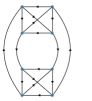
Figure 4: The spinfoam 2–complex $\mathcal{C}$ (left) and its oriented boundary graph $\Gamma=\partial\mathcal{C}$ (right) chosen in christodoulou_planck_2016 . The four middle links (faces) carry the boundary data $\omega_{\Delta}$ and $\zeta_{\Delta}$ that correspond to a discretization of the sphere $\Delta$, defined as the intersection of $\mathcal{C^{\pm}}$. The six upper and six lower links (faces) carry the boundary data $\omega_{\pm}$ and $\zeta_{\pm}$ respectively, that correspond to a particularly rough discretization of the remaining of the surfaces $\mathcal{C}^{\pm}$ while the surfaces $\mathcal{F}^{\pm}$ were disregarded. It is striking that this rough discretization gives exactly the behavior for the bounce time $T_{c}$ and lifetime $\tau$ expected on general grounds from the analysis in Section V. This should be taken as an indication that the relevant physics happen in the vicinity of the sphere $\Delta$, see mariosInfoParadox for a detailed argument.

The boundary data $\omega_{\ell}$ and $k_{\ell\mathrm{n}}$ in christodoulou_planck_2016 correspond to a critical point for the partial amplitude that reconstructs a degenerate 3d geometry. That is, two 4–simplices with triangle areas $\omega_{\ell}\,\hbar$ and face normals $k_{\ell\mathrm{n}}$ as in christodoulou_planck_2016 , and glued along one of their five tetrahedra so that they correspond to a simplicial manifold dual to the spinfoam in Figure 4, have zero 4–volume. This can be checked explicitly by calculating the edge lengths of the 4–simplices from $\omega_{\ell}$ and $k_{\ell\mathrm{n}}$, and then calculating their 4–volume written as a Cayley–Menger determinant, verifying that it vanishes. The vanishing of the 4–volume follows from the fact that the triangulation is taken to be intrinsically flat: the five tetrahedra making up each four simplex glue properly when embedded in a 3d Euclidean space. They correspond to a tetrahedron split in four tetrahedra with all deficit angles on the interior edges equal to zero. Thus, when promoted to a 4–simplex, this is a degenerate 4–simplex. For an analogy in one dimension lower, think of a tetrahedron with three of its triangles in the plane of the fourth triangle. This can be understood either as a 2d geometry made up of three triangles, or, as a 3d geometry made up of one tetrahedron of zero 3–volume.

We saw in Section V that the estimates for $T_{c}$ and $\tau$ are not affected by the kind of geometrical critical point for the partial amplitude. Then, the fact that the chosen boundary data correspond to a degenerate 4d triangulation can be seen as an (accidental) smart choice, that allows to understand easily equations (60) and (61). All dihedral angles $\phi_{\ell}(\delta_{\ell})$ will vanish, there is only a $\Pi_{\ell}=\pi$ thin–wedge contribution at $\Delta$ to consider on top of the embedding data $\zeta_{\ell}$. The dihedral angles $\phi(\delta_{\ell})$ are calculated using well known trigonometry formulas, see for instance dittrich_area-angle_2008-1 .

Setting $\phi_{\ell}(\delta_{\ell})=0$ for all $\ell$ and neglecting the sum over co–frame orientations $s(v)$ and the scaling $\lambda^{2M}$ of (V), the transition amplitude then scales as

$$W(m,T)\sim e^{-\frac{4}{t(m)}\left(\gamma\frac{T}{2m}-\pi\right)^{2}}e^{-\frac{12}{t(m)}\left(\zeta^{\pm}\right)^{2}},$$ (62)

with the factors $4$ and $12$ coming from the number of corresponding links in the boundary graph. Then, the crossing time can be read off directly from this expression as $T_{c}=2\pi m/\gamma$, in agreement with the numerical estimate in equation (60). Setting $T=T_{c}$, we have

$$|W(m,T_{c})|^{2}\sim e^{-\frac{24}{t(m)}\,\left(\zeta^{\pm}\right)^{2}}.$$ (63)

Thus the lifetime will scale as $\tau(m)\sim e^{\frac{\Xi}{t(m)}}$ with $\Xi=24\,(\zeta^{\pm})^{2}\approx 1820$, in agreement with equation (61).

These results are verified numerically in the figures below. We briefly summarize their content with further details given in their description. The amplitude estimate is shown in Figure 5. We see that a pronounced peak is present in the interval of the bounce time $T$ for which the estimate is reliable. The value of $T$ at the peak is the crossing time $T_{c}$. In Figure 6 we verify that $T_{c}$ is given by $T=2\pi/\gamma$. In the following two figures we show that the lifetime scales as $\tau(m)\sim e^{-\Xi/t(m)}$ with $\Xi$ a positive constant. Instead of $\tau(m)$, we plot $-t(m)\log\tau(m)$ against $m$. In Figure 7 we see that $-t(m)\log\tau(m)$ is constant in the mass $m$ and does not depend on the power $n$. In Figure 8 we verify that for $t=m^{2}/\hbar$, $\Xi$ scales as the inverse of $\hbar$.

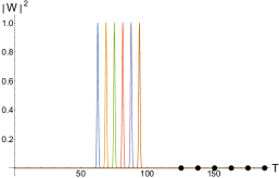
Figure 5: The modulus squared of the transition amplitude $W(m,T)$ for mass values $m=10,11,\dots,15$. The peak in the bounce time $T$ is at $T_{c}=2\pi m/\gamma$ and corresponds to the crossing time, see also Figure 6. The peak is normalized to unit for presentation purposes. The semiclassicality parameter is fixed to $t=\hbar/m^{2}$ ($n=2$) and the Immirzi parameter to $\gamma=1$. The bold black dots on the horizontal axis mark the maximal value of $T$ for which the estimate for the transition amplitude of equation (V) is valid, as a result of the truncation. According to equations ​ (31) and (59), the estimate is valid in the interval $0\leq T\leq 4\pi m/\gamma$.

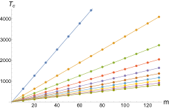
Figure 6: The crossing time $T_{c}$ for mass values $m=10,20,\ldots,130$ and for different values of the Immirzi parameter, $\gamma=0.1,0.2,\ldots,1$. The interpolation is $2\pi m/\gamma$. Numerical tests for different powers $n$ for the semiclassicality parameter $t=m^{-n}$ and different values for the Planck constant $\hbar$ give identical results, verifying that $T_{c}$ does not depend on $t$ and does not scale with $\hbar$.

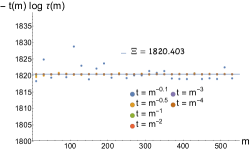
Figure 7: This and the following two figures show that the lifetime scales as $\tau(m)\sim e^{-\Xi/t(m)}$, where $\Xi$ is to a very good approximation a positive constant for the permissible values for the semiclassicality parameter $t(m)$. The estimate in eq.​ (V) begins to break down when $n$ approaches the lower limit of eq.​ (55). This effect is visible in the data set for $t=m^{-0.1}$ and $\hbar=1$ (blue), which nevertheless gives $\Xi$ a constant within 1%. The other data sets overlap within at least 0.1% accuracy.

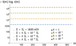
Figure 8: In this plot we verify that, as expected dimensionally, $\Xi$ scales as $\hbar^{-1}$. The vertical axis is logarithmic. The semiclassicality parameter is fixed to $t=m^{-2}$ ($n=2$) and the Immirzi parameter $\gamma$ is set to unit. The lifetime $\tau(m)$ goes to infinity as $\hbar\rightarrow 0$. Numerical tests for different values for the Immirzi parameter $\gamma$ give identical results, verifying that $\Xi$ does not depend on $\gamma$.

Appendix B Scaling of the Geometry in $m$ and $T$ and Monotonicity of Boost Angles

In this appendix we discuss the scaling of geometrical quantities with respect to the spacetime parameters of the HR metric. In particular, we show that any boost angle $\xi$ between two timelike vectors $n_{i}^{\alpha}=(n_{i}^{v},n_{i}^{r},0,0)$, $i=1,2$, will scale monotonically with $X\equiv T/m$, as well as with $T$ and $m$ separately. Concretely, we find that

$$\mathrm{sign}\frac{\mathrm{d}\,\xi}{\mathrm{d}X}=-\mathrm{sign}f,$$ (64)

where $f$ is the Schwarzschild lapse function. Thus, the scaling behavior is inverted when considering a boost angle calculated inside or outside the horizon, decreasing or increasing accordingly with $X$. We conclude that $\frac{\mathrm{d}\xi}{\mathrm{d}X}=0$ is an equivalent characterization of the $r=2m$ hypersurfaces in the HR spacetime:

$$\frac{\mathrm{d}\xi(r)}{\mathrm{d}X}=0\quad\Leftrightarrow\quad r=2m,$$ (65)

where $\xi$ is any boost angle calculated at a point with coordinate radius $r$. This scaling behavior demonstrates that the embedding data $\zeta_{\ell}$ can encode the presence of the (anti–) trapped surfaces $\mathcal{C}^{\pm}$.

For definiteness, we take $n_{i}^{\alpha}$ to be both past or future oriented (thick–wedge). The case of normals with opposite time orientation (thin–wedge) proceeds similarly. See Chap.​​ 4 of mariosPhd for the role of the two cases in the Lorentzian Regge action.

The boost angle $\xi$ is given by

$$\xi=\mathrm{arcosh}\,-\frac{g(n_{1},n_{2})}{|n_{1}|\,|n_{2}|},$$ (66)

where $|n_{i}|\equiv\sqrt{-g(n_{i},n_{i})}$ and the inner product is taken with the metric $g$. The inverse hyperbolic cosine is a real strictly monotonically increasing function when its argument is larger or equal to one, which is the case here. Specifically,

$$I\equiv-\frac{g(n_{1},n_{2})}{|n_{1}|\,|n_{2}|}\in(1,\infty),$$ (67)

with $I=1$ excluded because $n_{1}$ and $n_{2}$ are taken to be different vectors. Then, to conclude that boost angles scale monotonically in $X$, it suffices to show that $I$ is a monotonic function of $X$.

We want to examine the scaling of a boost angle as we move through the family of HR spacetimes, that is, as we vary $m$ and $T$. Then, the definition of the locus at which the boost angle $\xi$ is calculated cannot depend on $m$ or $T$. The same is true for other geometrical invariants, such as proper areas etc.​ A simple way to achieve this is to use dimensionless coordinates, adapted to the spacetime parameters. As an example, consider the Schwarzschild line element in ingoing EF coordinates. Applying the coordinate transformation $r\rightarrow\tilde{r}\equiv r/m$ and $v\rightarrow\tilde{v}\equiv v/m$, we have

$$\mathrm{d}s^{2}=m^{2}\left[-\left(1-\frac{2}{\tilde{r}}\right)\mathrm{d}\tilde{v}^{2}+2\mathrm{d}\tilde{v}\,\mathrm{d}\tilde{r}+\tilde{r}^{2}\mathrm{d}\Omega^{2}\right].$$ (68)

Therefore any invariant integral taken on a submanifold of dimension $D=1,2,3,4$ will be equal to a factor $m^{D}=\sqrt{m^{2D}}$, coming from the square root of the induced metric, times an integral that does not depend on $m$. That is, areas scale with $m^{2}$, proper lengths and times with $m$ etc. Since $m^{2}$ is a global conformal factor in the above line element, angles do not scale with $m$.

The same trick can be done with the HR metric, by defining

$$\tilde{r}=\frac{r}{m}\;,\quad\tilde{v}=\frac{v}{T}.$$ (69)

Then, the location of the shell is independent of $m$ and $T$ because

$$\Theta\left(v+\frac{T}{2}\right)=\Theta\left(T\tilde{v}+\frac{T}{2}\right)=\Theta\left(\tilde{v}+\frac{1}{2}\right),$$ (70)

and the metric (III.2) reads

$$\mathrm{d}s^{2}=m^{2}\bigg{[}-f(\tilde{r},\tilde{v})X^{2}\mathrm{d}\tilde{v}^{2}+2X\mathrm{d}\tilde{v}\,\mathrm{d}\tilde{r}+\tilde{r}^{2}\mathrm{d}\Omega^{2}\bigg{]},$$ (71)

where we defined

$$f(\tilde{r},\tilde{v})\equiv 1-\frac{2}{\tilde{r}}\,\Theta\left(\tilde{v}+\frac{1}{2}\right).$$ (72)

We emphasize that the above form of the metric shows that the scaling behaviors discussed here concern the entire spacetime, they hold also for the flat regions $I$ and $IV$. We read off for instance that areas scale as $m^{2}\delta(X)$ where $\delta$ is some function of $X$. Similarly, $m^{2}$ is no longer a global conformal factor and angles are in general functions of $X$, scaling with both $m$ and $T$.

After these preliminary considerations we may now show equation (64). The function $I(X)$ depends only on $X$ because the overall $m^{2}$ factor in the metric cancels in equation (67). Take the point where the boost angle $\xi$ is being calculated to be given by some $\tilde{r}=\tilde{R}$, $\tilde{v}=\tilde{\cal{V}}$ and constant $\theta,\phi$. For conciseness, we denote $f\equiv f(\tilde{R},\tilde{\cal{V}})$ and define $N_{1}\equiv n_{1}^{r}/n_{1}^{v}$ and $N_{2}\equiv n_{2}^{r}/n_{2}^{v}$.

Then, a few lines of algebra show that

$$I(X)=\frac{F_{1}+F_{2}}{2\sqrt{F_{1}\,F_{2}}},$$

where the functions $F_{i}$ are given by

$$F_{i}=fX-2N_{i}=\frac{|n_{i}|^{2}}{X(n_{i}^{v})^{2}}.$$ (73)

The first equality above gives $\frac{\mathrm{d}F_{i}}{\mathrm{d}X}=f$, and from the second equality we see that the functions $F_{i}$ are strictly positive. A simple application of the chain rule then gives

$$\frac{\mathrm{d}I(X)}{\mathrm{d}X}=\frac{f}{\sqrt{F_{1}\,F_{2}}}\big{(}1-I(X)\big{)}.$$ (74)

The term in parenthesis is strictly negative because of Eq.​ (67). Thus, we have shown Eq.​ (64).

Appendix C Crossed Fingers: Mapping the HR Metric on the Kruskal Manifold

Here, we briefly discuss the mapping of the HR metric to the Kruskal manifold employed in haggard_quantum-gravity_2015 for the construction of the HR spacetime, which we call the “crossed fingers” mapping. We relate this construction to that of Section III, and give the relation between the bounce time $T$ and the parameter $\delta$ used in haggard_quantum-gravity_2015 . The parameter $\delta$ determines where the two null shells intersect in the “crossed fingers” mapping.

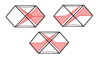
Figure 9: Some of the possible mappings of the two Kruskal patches of the HR spacetime to the full Kruskal manifold. See Figure 10 for a detailed breakdown of a single patch. It is impossible to map the HR spacetime to the Kruskal manifold using a single patch: the patches either overlap or are disjoint. Thus, we need to use at least two distinct patches. The upper–left case is the “crossed fingers” diagram, which corresponds to the construction originally employed in haggard_quantum-gravity_2015 and to the junction condition used here, see equation (9).

In Section III we described the HR metric using two different patches from the Kruskal manifold, one for region $II$ and one for region $III$ of the Carter–Penrose diagram of Figure 2. This is necessary because there does not exist an injective map from the union of regions $II$ and $III$ of the HR spacetime to a region of the Kruskal manifold. Different mappings are possible, all leading to the two patches either overlapping patches or being disjoint, see Figure 9 and its description. The junction condition given in equation (9) corresponds to the “crossed fingers” mapping, depicted on the top left of Figure 9 and in more detail in Figure 10.

We have seen that the HR metric depends on two physical scales, the mass $m$ and the bounce time $T$. The mass $m$ is implied by the use of the Kruskal manifold. The bounce time $T$, is encoded in the radius at which the two null shells cross in the “crossed fingers” mapping of the HR spacetime to the Kruskal manifold. We call this radius $r_{\delta}$ and the sphere at their intersection $\delta$. The ingoing and outgoing EF coordinates of the sphere $\delta$ are given by $v_{\mathcal{S}^{-}}$ and $u_{\mathcal{S}^{+}}$. From equation (14), we infer the relation

$$T=-2r^{\star}(r_{\delta}).$$ (75)

We conclude that it is equivalent to consider the area corresponding to the radius $r_{\delta}$ as the second spacetime parameter for the HR metric.

By a slight abuse of notation we introduce the parameter $\delta>0$ for the sphere $\delta$ at radius $r_{\delta}$, defined by

$$r_{\delta}=2m\left(1+\delta\right).$$ (76)

The bounce time $T$ and $\delta$ are then related by

$$e^{-\frac{T}{4m}}=\delta\,e^{1+\delta},$$ (77)

where we used $r^{\star}(r)=r+2m\log|\frac{r}{2m}-1|$. This relation is solved for $\delta$ by the Lambert $W$ function

$$\delta=W\left(\frac{e^{-\frac{T}{4m}}}{e}\right).\$$ (78)

The condition that the bounce time $T$ is positive translates into

$$\delta<W\!\left(1/e\right)\approx 0.28.$$ (79)

An infinite bounce time corresponds to a vanishing $\delta$. Thus, we may use as parameters for the HR spacetime the mass $m$, constrained to be positive, and the parameter $\delta$, constrained to lie in the interval

$$\delta\in\big{(}\,0,W\!\left(1/e\right)\,\big{)}.$$ (80)

Figure 10: The two Kruskal patches of the Haggard–Rovelli spacetime (color online) in the “crossed fingers” mapping, see top left of Figure 9. Each patch (shaded) is bounded by a null shell $\mathcal{S^{\pm}}$ (red), by a boundary surface $\mathcal{C^{\pm}}$ (green), by the fiducial surface $\mathcal{T}$ (blue) along which the two patches are joined via the junction condition of eq.​ (9), and by a portion of $\cal{J}^{\pm}$. The geometry of the patch on the left is given by the line elements of eqs. (III.2) and (III.2). The geometry of the patch on the right is given by the line elements of eqs. (III.2) and (III.2).

Appendix D The Bounce Time $T$ as an Interval at Null Infinity

D.1 The Bounce Time $T$ as an Evaporation Time and a Convenient Value for $r_{\Delta}$

The bounce time $T$ can be understood as an interval of an affine parameter on $\cal{J}^{+}$. We will show that it is a concept analogous to the Hawking evaporation time. Despite the fact that Hawking evaporation has been neglected in this work, this alternative point of view is desirable for two reasons. First, it implies that we can directly compare time scales such as the lifetime and the crossing time, which are values for $T$, to the Hawking evaporation time scale $\sim m^{3}$. Second, the protrusion of the quantum region outside the trapped surfaces will interfere with the definition of the “first” Hawking photon. We will see that certain constraints arise and verify that they are mild and consistent with relevant literature.

An affine parameters on $\cal{J}^{+}$ is provided by the outgoing EF coordinate $u_{\mathcal{S}^{+}}$. From (14) we see that by defining an asymptotic time

$$u_{fhp}=v_{\mathcal{S}^{-}},$$ (81)

in outgoing EF coordinates for the regions $III$ and $IV$, the bounce time corresponds to the interval

$$T=u_{\mathcal{S}^{+}}-u_{fhp}$$ (82)

on $\cal{J}^{+}$. The asymptotic time $u_{fhp}$ is light traced in the past either on the boundary surface $\mathcal{C}^{+}$, in which case the ray is not extendible outside region $III$, or, it will cross to region $II$, then to region $I$ and be light traced all the way to $\cal{J}^{-}$.

In the latter case, the light ray $u_{fhp}$ intersects the collapsing shell $\mathcal{S^{-}}$ and allows us to establish an analogy to the Hawking evaporation time. Demanding that $u_{fhp}$ is light traced to $\cal{J^{-}}$, is equivalent to imposing

$$u_{\Delta}\geq u_{fhp}.$$ (83)

We will turn the above inequality into a condition for the area of the sphere $\Delta$. We first trivially extend the outgoing EF coordinates of regions $III$ and $IV$ to region $II$ using the relation $v-u=2r^{\star}(r)$ between the coordinates $(v,r)$ and $(u,r)$, and the junction condition (9). The new $(u,r)$ coordinate system covers the relevant portion ($u\leq u_{\Delta}$) of region $II$. Because the boundary $\mathcal{B}$ is arbitrary, we can only write down a necessary condition for equation (83) to hold:

$$r^{\star}(r_{\Delta})\leq 0.$$ (84)

This is shown as follows,

$$r^{\star}(r_{\Delta}) \leq 0$$

$$\Rightarrow v_{\Delta}-u_{\Delta} \leq 0\leq v_{\Delta}-v_{\mathcal{S}^{-}}$$

$$\Rightarrow\ u_{\Delta} \geq v_{\mathcal{S}^{-}},$$ (85)

where we used that $v_{\Delta}-v_{\mathcal{S}^{-}}\geq 0$.

It is convenient to define a parameter $\Delta$ by

$$r_{\Delta}=2m\,(1+\Delta)\quad,\quad\Delta>0.$$ (86)

Note the abuse of notation: $\Delta$ denotes both, the sphere at the intersection of $\mathcal{C}^{\pm}$ and the positive number $\Delta$ related to its area by $A_{\Delta}=4\pi\,(2m)^{2}(1+\Delta)^{2}$. The equation $r^{\star}(r_{\Delta})=0$ reads

$$1+\Delta+\log\Delta=0,$$ (87)

and after exponentiation we have

$$\Delta\,e^{\Delta}=1/e.$$ (88)

The formal solution $\Delta_{0}$ to this equation is given by the Lambert $W$ function

$$\Delta_{0}=W(1/e)\approx 0.28,$$ (89)

and we call the corresponding radius $r_{0}$

$$r_{0}=2m(1+\Delta_{0})\approx 2.56m.$$ (90)

It follows that

$$r_{\Delta}\leq r_{0}\quad\Rightarrow\quad u_{\Delta}\geq u_{fhp},$$ (91)

because $r^{\star}$ is monotonically increasing in $r$.

We now consider the sphere defined as the intersection of the null hypersurface given by $u=u_{fhp}$ and the collapsing shell $\mathcal{S}^{-}$ which sits at $v=v_{\mathcal{S}^{-}}$. This sphere is in region $II$. Call the value of the radial coordinate on that sphere $r_{fhp}$. Since $u_{fhp}=v_{\mathcal{S}^{-}}$ and using $v-u=2r^{\star}(r)$, we have

$$r^{\star}(r_{fhp})=0,$$ (92)

that is,

$$r_{fhp}=r_{0}.$$ (93)

The condition of eq.​ (91) is now easy to read from a Carter–Penrose diagram. The ray $u_{fhp}$ is outgoing in the asymptotic region of the HR spacetime where the expansion of outgoing null geodesics is positive, and thus cannot intersect the sphere $\Delta$ at a greater radius than its intersection with $\mathcal{S}^{-}$. That is, if $r_{\Delta}\leq r_{fhp}=r_{0}$ holds, the light ray $u_{fhp}$ can be light traced to $\mathcal{S}^{-}$.

The above imply that when eq.​ (91) holds, the bounce time $T$ is analogous to an evaporation time. An evaporation time is defined as the time measured at infinity between the reception of the “first” and “last” Hawking photon. The analogue of the “last” Hawking photon is here the outgoing shell $\mathcal{S}^{+}$. A precise definition for the “first” Hawking photon can be found in bianchi_entanglement_2014 . In that work, the authors defined $u_{fhp}$ as marking the onset of entanglement entropy production at $\cal{J}^{+}$. They estimated the radius at which it is most likely for the first Hawking photon to be emitted to be roughly when the collapsing shell reaches a radius $\sim 3m$. An ambiguity of order one in the coefficient multiplying $m$ will typically be involved in defining the emission of the first Hawking photon.

In summary, by fixing $r_{\Delta}=r_{0}\approx 2.58m$, the bounce time corresponds to the interval $T=u_{\mathcal{S}^{-}}-u_{fhp}$ of the affine parameter $u$ at $\cal{J}^{+}$ and $u_{fhp}$ can be light traced to $\mathcal{S}^{-}$. The ray $u_{fhp}$ labels the sphere on $\mathcal{S}^{-}$ with radius $r_{fhp}=r_{0}$, a reasonable value for defining the emission of the first Hawking photon. Taking $r_{\Delta}=r_{0}$ for the extent of the quantum region does not appear restrictive. In haggard_quantum-gravity_2015 the quantum effects were estimated to be most pronounced at a radius $\frac{7}{6}2m\approx 2.33m$. We see in the following section that fixing $r_{0}=r_{\Delta}$ is also convenient for other reasons.

Of course, if Hawking evaporation is considered care must be taken for the relevant time regimes for which the metric of Section III is a valid approximation. The discussion here makes clear that the mass loss due to Hawking evaporation can be neglected when $T\ll m^{3}$.

D.2 Duration of Black and White Phases and Positivity of the Bounce Time $T$

Following de_lorenzo_improved_2016 ; bianchi_entanglement_2014 , the duration of the trapped and anti–trapped phase can be encoded in two intervals $\delta v$ and $\delta u$ respectively, defined as

$$\delta v \equiv v_{\Delta}-v_{\mathcal{S^{-}}}$$

$$\delta u \equiv u_{\mathcal{S^{+}}}-u_{\Delta}.$$ (94)

The meaning of $\delta v$ and $\delta u$ is as follows: For given surfaces $\mathcal{C}^{-}$ and $\mathcal{C}^{+}$, and for fixed $\delta v$ and $\delta u$, the endpoints of the portion of the $r=2m$ correspond to intervals at $\cal{J}^{-}$ and $\cal{J}^{-}$ bounded from above by $\delta v$ and $\delta u$, respectively. This can be read from Figures 9 and 10, we recall that the surfaces $\mathcal{C}^{\pm}$ are spacelike.

Using $v-u=2r^{\star}(r)$, $\delta v$ and $\delta u$ are related to the bounce time by

$$T=\delta v+\delta u-2r^{\star}(r_{\Delta}).$$ (95)

Thus, a given value for $T$ allows for different durations of the black and white hole phase. The term $-2r^{\star}(r_{\Delta})$ is linear in $m$ and is negligible for $T\gg m$. However, this term is negative for $r_{\Delta}>r_{0}$, and to guarantee the strict positivity of $T$ we must demand that

$$\delta_{v}+\delta_{v}>2r^{\star}(r_{\Delta})\sim m.$$ (96)

This is a mild condition to impose. For example, a time of order $m$ for a solar mass black hole is of the order of a microsecond, and about a second for Sagittarius $A^{\star}$. However, fixing $r_{\Delta}=r_{0}$ as in the previous section is again convenient. The bounce time becomes exactly the sum of $\delta v$ and $\delta u$

$$T=\delta v+\delta u.$$ (97)

Since the inequalities (III.2) ensure that $\delta v$ and $\delta u$ are always positive, $T$ is also positive

$$T>0.$$ (98)

Appendix E The HR metric in Kruskal Coordinates

In this Appendix we give the HR metric in Kruskal null coordinates, for easier comparison with the discussion in reference haggard_quantum-gravity_2015 . We install null Kruskal coordinate systems $(U_{i},V_{i})$, $i=I,II,III,IV$, in all four regions of the Carter–Penrose diagram in Figure 2. The metric reads

$$\mathrm{d}s^{2}=-F_{i}(U_{i},V_{i})\,\mathrm{d}U_{i}\,\mathrm{d}V_{i}+r^{2}_{i}(U_{i},V_{i})\,\mathrm{d}\Omega^{2}.\quad$$

In regions $I$ and $IV$ we have the flat line element

$$F_{i}(U_{i},V_{i}) = 1,$$

$$r_{i}(U_{i},V_{i}) = \frac{V_{i}-U_{i}}{2},$$

and in regions $II$ and $III$ the Kruskal line element

$$F_{i}(U_{i},V_{i}) = \frac{32\,m^{3}}{r_{i}}\operatorname{e}^{-\frac{r_{i}}{2m}},$$

$$r_{i}(U_{i},V_{i}) = 2m\,\left(W\left(-\frac{U_{i}V_{i}}{\operatorname{e}}\right)+1\right),$$

where $W$ is the Lambert function.

The junction conditions for the intrinsic metric on $\mathcal{T}$ are trivially satisfied by identifying the coordinates of the charts in region $II$ and $III$,

$$U_{\rm III}\stackrel{{\scriptstyle\mathcal{T}}}{{=}}U_{\rm II},$$

$$V_{\rm III}\stackrel{{\scriptstyle\mathcal{T}}}{{=}}V_{\rm II}.$$ (99)

The position of the null shells $\mathcal{S^{-}}$ and $\mathcal{S}^{+}$ in these coordinates is denoted as $V_{S}^{-}$ and $U_{S}^{+}$ respectively. The junction condition for the intrinsic metric on $\mathcal{S^{\pm}}$ ensures that the spheres foliating these surfaces have the same area as seen by the metrics on both sides. That is, the values of the radius function on either side of $\mathcal{S^{\pm}}$ are identified. For $\mathcal{S^{-}}$, we have

$$r_{\rm I}(U_{\rm I},V_{\rm I}=V_{\mathcal{S^{-}}})=r_{\rm II}(U_{\rm II},V_{\rm II}=V_{\mathcal{S^{-}}}).$$

Equivalently,

$$V_{\rm I} \stackrel{{\scriptstyle\mathcal{S^{-}}}}{{=}} V_{\rm II}\stackrel{{\scriptstyle\mathcal{S^{-}}}}{{=}}V_{\mathcal{S^{-}}}$$

$$U_{\rm II} \stackrel{{\scriptstyle\mathcal{S^{-}}}}{{=}} \frac{1}{V_{\mathcal{S^{-}}}}\left(1-\frac{V_{\mathcal{S^{-}}}-U_{\rm I}}{4m}\right)\operatorname{e}^{\frac{V_{\mathcal{S^{-}}}-U_{\rm I}}{4m}}.$$

Similarly, on $\mathcal{S^{+}}$ we have the identification

$$r_{\rm III}(U_{\rm III}=U_{\mathcal{S^{+}}},V_{\rm III})=r_{\rm IV}(U_{\rm IV}=U_{\mathcal{S^{+}}},V_{\rm IV}),$$

which gives

$$U_{\rm III} \stackrel{{\scriptstyle\mathcal{S^{+}}}}{{=}} U_{\rm IV}\stackrel{{\scriptstyle\mathcal{S^{+}}}}{{=}}U_{\mathcal{S^{+}}}$$

$$V_{\rm III} \stackrel{{\scriptstyle\mathcal{S^{+}}}}{{=}} \frac{1}{U_{\mathcal{S^{+}}}}\left(1-\frac{V_{\rm IV}-U_{\mathcal{S^{+}}}}{4m}\right)\operatorname{e}^{\frac{V_{\rm IV}-U_{\mathcal{S^{+}}}}{4m}}.$$

For a given interior boundary, the ranges of coordinates are given by the conditions

$$V\!\in\!(-\infty,V_{\mathcal{S^{-}}}),\ U\!\in\!(-\infty,\infty),\ \ \ U\!\leq\!\mathcal{F^{-}}(V)$$

$$V\!\in\!(V_{\mathcal{S^{-}}},\infty),\ \ \ U\!\in\!(-\infty,\infty),\ \ \ U\!\leq\!\mathcal{C^{-}}(V),\ \ U\!\leq\!\mathcal{T^{-}}(V)$$

$$V\!\in\!(-\infty,\infty),\ \ \ U\!\in\!(-\infty,U_{\mathcal{S^{+}}}),\ U\!\geq\!\mathcal{C^{+}}(V),\ U\!\geq\!\mathcal{T^{+}}(V)$$

$$V\!\in\!(-\infty,\infty),\ \ \ U\!\in\!(U_{\mathcal{S^{+}}},\infty),\ \ \ U\!\geq\!\mathcal{F^{+}}(V).$$

for the patch $I,II,III,IV$ respectively.

The coordinates of the sphere $\Delta$ must satisfy

$$0<V_{\mathcal{S^{-}}}<V_{\Delta}$$

$$U_{\Delta}<U_{\mathcal{S^{+}}}<0$$

and, in order to ensure the presence of trapped and anti–trapped regions in the spacetime, we impose the inequalities $r_{\epsilon^{\pm}}<2m$ and $r_{\Delta}>2m$, as in (III.2).

The transformation between Kruskal and EF coordinates on each patch is given by $V=\operatorname{e}^{\frac{v}{4m}}$ and $U=-\operatorname{e}^{\frac{-u}{4m}}$. With respect to the metric of Section III we have

$$v_{\mathcal{S}^{-}} = 4m\log V_{\mathcal{S^{-}}},$$

$$u_{\mathcal{S}^{+}} = -4m\log-U_{\mathcal{S}^{+}}.$$

The bounce time in terms of $V_{\mathcal{S}}^{-}$ and $U_{\mathcal{S}}^{+}$ is then given by

$$T=4m\log\left(-\frac{V_{\mathcal{S}}^{-}}{U_{\mathcal{S}}^{+}}\right).$$

References

- (1) S. W. Hawking, Black hole explosions?, Nature 248 (Mar., 1974) 30–31.
- (2) H. M. Haggard and C. Rovelli, Quantum-gravity effects outside the horizon spark black to white hole tunneling, Phys.Rev. D92 (Nov., 2015) 104020.
- (3) D. Malafarina, Classical collapse to black holes and quantum bounces: A review, Universe 3 (2017) 48.
- (4) T. De Lorenzo and A. Perez, Improved Black Hole Fireworks: Asymmetric Black-Hole-to-White-Hole Tunneling Scenario, Physical Review D 93 (June, 2016) [1512.04566].
- (5) C. W. Misner, Feynman Quantization of General Relativity, Reviews of Modern Physics 29 (July, 1957) 497–509.
- (6) M. Christodoulou, C. Rovelli, S. Speziale and I. Vilensky, Planck star tunneling time: An astrophysically relevant observable from background-free quantum gravity, Phys.Rev. D94 (Oct., 2016) 084035.
- (7) M. Christodoulou and F. D’Ambrosio, Towards gravitational tunneling in spinfoams, to appear.
- (8) M. Christodoulou, Geometry Transition in Covariant Loop Quantum Gravity. PhD thesis, Marseille, Oct. 2017. [1803.00332]
- (9) S. Hawking and G. Ellis, The Large Scale Structure of Space-Time, Appendix B. Cambridge University Press, 1975.
- (10) P. Vaidya, The Gravitational Field of a Radiating Star, Proc.Natl.Inst.Sci.India A33 (1951) 264.
- (11) E. Poisson, A Relativist’s Toolkit, Section 3.7 and Section 5.1.8. Cambridge University Press, 2004.
- (12) M. Blau, Lecture notes in general relativity, section 31.9 and section 39.9, .
- (13) E. Bianchi, T. De Lorenzo and M. Smerlak, Entanglement entropy production in gravitational collapse: Covariant regularization and solvable models, arXiv:1409.0144 [gr-qc, physics:hep-th] (Aug., 2014) [1409.0144].
- (14) R. Oeckl, A ”general boundary” formulation for quantum mechanics and quantum gravity, Physics Letters B 575 (Nov., 2003) 318–324 [hep-th/0306025].
- (15) R. Oeckl, General boundary quantum field theory: Foundations and probability interpretation, arXiv:hep-th/0509122 (Sept., 2005) [hep-th/0509122].
- (16) C. Rovelli and F. Vidotto, Covariant Loop Quantum Gravity: An Elementary Introduction to Quantum Gravity and Spinfoam Theory. Cambridge University Press, Nov., 2014.
- (17) A. Perez, The Spin Foam Approach to Quantum Gravity, 1205.2019.
- (18) J. C. Baez, Spin foam models, Class.Quant.Grav. 15 (1998) 1827–1858.
- (19) A. Ashtekar, Introduction to Loop Quantum Gravity, 1201.4598.
- (20) T. Thiemann, Modern Canonical Quantum General Relativity. Cambridge University Press, Sept., 2007.
- (21) C. Rovelli, Quantum Gravity. Cambridge University Press, Nov., 2004.
- (22) R. Gambini and J. Pullin, A First Course in Loop Quantum Gravity. OUP Oxford, Sept., 2011.
- (23) A. Barbieri, Quantum tetrahedra and simplicial spin networks, Nucl.Phys. B518 (1998) 714–728.
- (24) J. C. Baez and J. W. Barrett, The Quantum tetrahedron in three-dimensions and four-dimensions, Adv.Theor.Math.Phys. 3 (1999) 815–850.
- (25) E. Bianchi, P. Dona and S. Speziale, Polyhedra in loop quantum gravity, Phys.Rev. D83 (2011) 044035.
- (26) H. M. Haggard, Pentahedral volume, chaos, and quantum gravity, Phys.Rev. D87 (Feb., 2013) 044020.
- (27) G. Ponzano and T. Regge, Semiclassical Limit of Racah Coefficients., pp 1-58 of Spectroscopic and Group Theoretical Methods in Physics. Block, F. (ed.). New York, John Wiley and Sons, Inc., 1968. (Oct., 1969).
- (28) T. Regge, General Relativity Without Coordinates, Nuovo Cim. 19 (1961) 558–571.
- (29) H. Ooguri, Partition Functions and Topology-Changing Amplitudes in the 3D Lattice Gravity of Ponzano and Regge, Nuclear Physics B 382 (Sept., 1992) 276–304 [hep-th/9112072].
- (30) C. Rovelli, The Basis of the Ponzano-Regge-Turaev-Viro-Ooguri quantum gravity model in the loop representation basis, Phys.Rev. D48 (1993) 2702–2707.
- (31) V. Turaev and O. Viro, State sum invariants of 3-manifolds and quantum 6j-symbols, Topology 31 (Oct., 1992) 865–902.
- (32) D. V. Boulatov, A Model of three-dimensional lattice gravity, Mod.Phys.Lett. A7 (1992) 1629–1646.
- (33) J. W. Barrett and L. Crane, A Lorentzian Signature Model for Quantum General Relativity, Classical and Quantum Gravity 17 (Aug., 2000) 3101–3118 [gr-qc/9904025].
- (34) E. R. Livine and S. Speziale, A new spinfoam vertex for quantum gravity, Physical Review D 76 (Oct., 2007) [0705.0674].
- (35) J. Engle, R. Pereira and C. Rovelli, Flipped spinfoam vertex and loop gravity, Nuclear Physics B 798 (July, 2008) 251–290 [0708.1236].
- (36) L. Freidel and K. Krasnov, A New Spin Foam Model for 4d Gravity, Classical and Quantum Gravity 25 (June, 2008) 125018 [0708.1595].
- (37) A. Baratin and D. Oriti, Group field theory and simplicial gravity path integrals: A model for Holst-Plebanski gravity, Physical Review D 85 (Feb., 2012) [1111.5842].
- (38) M. Dupuis, L. Freidel, E. R. Livine and S. Speziale, Holomorphic Lorentzian Simplicity Constraints, Journal of Mathematical Physics 53 (Mar., 2012) 032502 [1107.5274].
- (39) J. Engle, A spin-foam vertex amplitude with the correct semiclassical limit, Physics Letters B 724 (July, 2013) 333–337 [1201.2187].
- (40) E. Bianchi and A. Satz, Semiclassical regime of Regge calculus and spin foams, Nuclear Physics B 808 (Feb., 2009) 546–568 [0808.1107].
- (41) J. W. Barrett, R. J. Dowdall, W. J. Fairbairn, H. Gomes and F. Hellmann, Asymptotic analysis of the EPRL four-simplex amplitude, Journal of Mathematical Physics 50 (Nov., 2009) 112504 [0902.1170].
- (42) J. W. Barrett, W. J. Fairbairn and F. Hellmann, Quantum gravity asymptotics from the SU(2) 15j symbol, International Journal of Modern Physics A 25 (June, 2010) 2897–2916 [0912.4907].
- (43) J. W. Barrett, R. J. Dowdall, W. J. Fairbairn, F. Hellmann and R. Pereira, Lorentzian spin foam amplitudes: Graphical calculus and asymptotics, Classical and Quantum Gravity 27 (Aug., 2010) 165009 [0907.2440].
- (44) E. Magliaro and C. Perini, Emergence of gravity from spinfoams, EPL (Europhysics Letters) 95 (Aug., 2011) 30007 [1108.2258].
- (45) E. Magliaro and C. Perini, Curvature in spinfoams, Classical and Quantum Gravity 28 (July, 2011) 145028 [1103.4602].
- (46) M. Han and M. Zhang, Asymptotics of Spinfoam Amplitude on Simplicial Manifold: Euclidean Theory, Classical and Quantum Gravity 29 (Aug., 2012) 165004 [1109.0500].
- (47) M. Han and M. Zhang, Asymptotics of Spinfoam Amplitude on Simplicial Manifold: Lorentzian Theory, Classical and Quantum Gravity 30 (Aug., 2013) 165012 [1109.0499].
- (48) M. Han, Semiclassical Analysis of Spinfoam Model with a Small Barbero-Immirzi Parameter, Phys.Rev. D88 (Aug., 2013) 044051.
- (49) M. Han and T. Krajewski, Path Integral Representation of Lorentzian Spinfoam Model, Asymptotics, and Simplicial Geometries, Class.Quant.Grav. 31 (Nov., 2013) 015009.
- (50) J. Engle, I. Vilensky and A. Zipfel, The Lorentzian proper vertex amplitude: Asymptotics, Physical Review D 94 (Sept., 2016) [1505.06683].
- (51) M. Han, Einstein Equation from Covariant Loop Quantum Gravity in Semiclassical Continuum Limit, Phys.Rev. D96 (July, 2017) 024047.
- (52) B. Bahr, S. Kloser and G. Rabuffo, Towards a cosmological subsector of spin foam quantum gravity, Physical Review D 96 (2017) 086009.
- (53) B. Bahr and S. Steinhaus, Investigation of the Spinfoam Path integral with Quantum Cuboid Intertwiners, Physical Review D 93 (May, 2016) [1508.07961].
- (54) E. Bianchi and Y. Ding, Lorentzian spinfoam propagator, Physical Review D 86 (Nov., 2012) [1109.6538].
- (55) A. C. Shirazi, J. Engle and I. Vilensky, Hessian and graviton propagator of the proper vertex, Classical and Quantum Gravity 33 (Oct., 2016) 205010 [1511.03644].
- (56) E. Bianchi, E. Magliaro and C. Perini, LQG propagator from the new spin foams, Nucl.Phys. B822 (2009) 245–269.
- (57) E. Alesci and C. Rovelli, The complete LQG propagator: II. Asymptotic behavior of the vertex, Physical Review D 77 (Feb., 2008) [0711.1284].
- (58) E. Alesci and C. Rovelli, The complete LQG propagator: I. Difficulties with the Barrett-Crane vertex, Physical Review D 76 (Nov., 2007) [0708.0883].
- (59) E. Bianchi, L. Modesto, C. Rovelli and S. Speziale, Graviton propagator in loop quantum gravity, Classical and Quantum Gravity 23 (Dec., 2006) 6989–7028 [gr-qc/0604044].
- (60) B. Dittrich, From the discrete to the continuous: Towards a cylindrically consistent dynamics, New J.Phys. 14 (2012) 123004.
- (61) B. Dittrich, E. Schnetter, C. J. Seth and S. Steinhaus, Coarse graining flow of spin foam intertwiners, Phys.Rev. D94 (Dec., 2016) 124050.
- (62) D. Oriti, Group Field Theory and Loop Quantum Gravity, .
- (63) C. Rovelli and M. Smerlak, In quantum gravity, summing is refining, Classical and Quantum Gravity 29 (Mar., 2012) 055004 [1010.5437].
- (64) C. Charles and E. R. Livine, Ashtekar-Barbero holonomy on the hyperboloid: Immirzi parameter as a Cut-off for Quantum Gravity, arXiv:1507.00851 [gr-qc] (July, 2015) [1507.00851].
- (65) E. Bianchi, E. Magliaro and C. Perini, Coherent spin-networks, Physical Review D 82 (July, 2010) [0912.4054].
- (66) T. Thiemann, Gauge Field Theory Coherent States (GCS) : I. General Properties, Classical and Quantum Gravity 18 (June, 2001) 2025–2064 [hep-th/0005233].
- (67) T. Thiemann and O. Winkler, Gauge Field Theory Coherent States (GCS) : III. Ehrenfest Theorems, Classical and Quantum Gravity 18 (Nov., 2001) 4629–4681 [hep-th/0005234].
- (68) T. Thiemann and O. Winkler, Gauge Field Theory Coherent States (GCS) : II. Peakedness Properties, Classical and Quantum Gravity 18 (July, 2001) 2561–2636 [hep-th/0005237].
- (69) L. Freidel and S. Speziale, Twisted geometries: A geometric parametrisation of SU(2) phase space, Physical Review D 82 (Oct., 2010) [1001.2748].
- (70) L. Freidel and S. Speziale, From twistors to twisted geometries, Physical Review D 82 (Oct., 2010) [1006.0199].
- (71) C. Rovelli and E. Wilson-Ewing, Discrete Symmetries in Covariant LQG, Physical Review D 86 (Sept., 2012) [1205.0733].
- (72) M. Christodoulou, A. Riello and C. Rovelli, How to detect an anti-spacetime, Int.J.Mod.Phys. D21 (2012) 1242014.
- (73) G. Immirzi, Causal spin foams, .
- (74) M. Vojinovic, Cosine problem in EPRL/FK spinfoam model, General Relativity and Gravitation 46 (Jan., 2014) [1307.5352].
- (75) J. Engle, Proposed proper Engle-Pereira-Rovelli-Livine vertex amplitude, Phys.Rev. D87 (Apr., 2013) 084048.
- (76) A. Barrau, C. Rovelli and F. Vidotto, Fast Radio Bursts and White Hole Signals, Physical Review D 90 (Dec., 2014) [1409.4031].
- (77) A. Barrau, B. Bolliet, F. Vidotto and C. Weimer, Phenomenology of bouncing black holes in quantum gravity: A closer look, JCAP 1602 (Feb., 2016) 022.
- (78) A. Barrau and C. Rovelli, Planck star phenomenology, Phys.Lett. B739 (Dec., 2014) 405–409.
- (79) F. Vidotto, A. Barrau, B. Bolliet, M. Shutten and C. Weimer, Quantum-gravity phenomenology with primordial black holes, .
- (80) L. Modesto, Black hole interior from loop quantum gravity, Advances in High Energy Physics 2008 (2008) 1–12 [gr-qc/0611043].
- (81) R. Gambini and J. Pullin, An introduction to spherically symmetric loop quantum gravity black holes, AIP Conf.Proc. 1647 (Mar., 2015) 19–22.
- (82) A. Corichi and P. Singh, Loop quantization of the Schwarzschild interior revisited, Classical and Quantum Gravity 33 (Mar., 2016) 055006 [1506.08015].
- (83) J. Olmedo, S. Saini and P. Singh, From black holes to white holes: A quantum gravitational, symmetric bounce, Classical and Quantum Gravity 34 (Nov., 2017) 225011 [1707.07333].
- (84) P. Hajicek and C. Kiefer, Singularity avoidance by collapsing shells in quantum gravity, International Journal of Modern Physics D 10 (Dec., 2001) 775–779 [gr-qc/0107102].
- (85) M. Ambrus and P. Hajicek, Quantum superposition principle and gravitational collapse: Scattering times for spherical shells, Phys.Rev. D72 (2005) 064025.
- (86) C. Barceló, R. Carballo-Rubio and L. J. Garay, Mutiny at the white-hole district, International Journal of Modern Physics D 23 (Oct., 2014) 1442022 [1407.1391].
- (87) C. Barceló, R. Carballo-Rubio, L. J. Garay and G. Jannes, The lifetime problem of evaporating black holes: Mutiny or resignation, Classical and Quantum Gravity 32 (Feb., 2015) 035012 [1409.1501].
- (88) C. Barceló, R. Carballo-Rubio and L. J. Garay, Black holes turn white fast, otherwise stay black: No half measures, Journal of High Energy Physics 2016 (Jan., 2016) [1511.00633].
- (89) C. Barceló, R. Carballo-Rubio and L. J. Garay, Exponential fading to white of black holes in quantum gravity, arXiv:1607.03480 [gr-qc, physics:hep-th] (July, 2016) [1607.03480].
- (90) E. Bianchi, M. Christodoulou, F. D’Ambrosio, H. Haggard and C. Rovelli, The surprising end of a black hole: Remnants are white holes, to appear.
- (91) B. Dittrich and S. Speziale, Area-angle variables for general relativity, New Journal of Physics 10 (Aug., 2008) 083006 [0802.0864].