Probabilistic performance estimators for computational chemistry methods:
the empirical cumulative distribution function of absolute errors

Abstract

Benchmarking studies in computational chemistry use reference datasets to assess the accuracy of a method through error statistics. The commonly used error statistics, such as the mean signed and mean unsigned errors, do not inform end-users on the expected amplitude of prediction errors attached to these methods. We show that, the distributions of model errors being neither normal nor zero-centered, these error statistics cannot be used to infer prediction error probabilities. To overcome this limitation, we advocate for the use of more informative statistics, based on the empirical cumulative distribution function of unsigned errors, namely (1) the probability for a new calculation to have an absolute error below a chosen threshold, and (2) the maximal amplitude of errors one can expect with a chosen high confidence level. Those statistics are also shown to be well suited for benchmarking and ranking studies. Moreover, the standard error on all benchmarking statistics depends on the size of the reference dataset. Systematic publication of these standard errors would be very helpful to assess the statistical reliability of benchmarking conclusions.

I Introduction

There is a wide gap between the information provided by benchmarking studies of computational chemistry (CC) methods and the information needed by end-users to choose a method adapted to their specific, application-dependent, requirements. It has been recently proposed that an unequivocal criterion matching both aims would be the prediction uncertainty Pernot et al. (2015); Proppe and Reiher (2017), which should enable to infer intervals around the predicted value in which the true value is expected to lie with a high probability Ruscic (2014). This would indeed be a valuable benchmarking and ranking criterion (the smaller, the better), and an essential information for users to select an adequate method (other rational criteria being, for instance, method availability and computational cost).

Prediction uncertainty is not always easy to estimate and requires a careful analysis of prediction errors, which are a mixture of modeling errors (method), discretization errors (basis set, grid…), numerical errors (floating-point arithmetic, convergence thresholds, stochastic algorithms…), with an added contribution of parametric uncertainty for semi-empirical methods Irikura, Johnson, and Kacker (2004); Cailliez and Pernot (2011). Model choice and discretization are mainly inducing systematic errors Dunning (2000); Pernot et al. (2015), while numerical and parametric sources are generally assumed to contribute randomly. For deterministic CC methods, numerical and parametric uncertainties are typically much smaller than systematic errors due to their founding approximations and discretization schemes Irikura, Johnson, and Kacker (2004); Pernot et al. (2015); Pernot (2017).

Estimation of prediction uncertainty requires the calculated values to be corrected, as well as possible, from systematic errors BIPM et al. (2008). This is achieved, for instance, by composite methods Pople et al. (1989); Raghavachari and Saha (2015), a posteriori correction estimated from trends in a calibration errors set Pernot et al. (2015); Simm and Reiher (2016), or machine learning Ramakrishnan et al. (2015); Rupp (2015). Prediction uncertainty is therefore expected to quantify the unpredictable part of prediction errors, which is observed in the residual errors after correction. Note that corrections are popular for some observables, such as vibrational frequencies, much less for other ones, such as atomization energies, and end-users most often use uncorrected results.

Current CC methods do not generally provide estimations of their prediction uncertainty, at the exception of the semi-empiric mBEEF density functional approximation (DFA) and its relatives Wellendorff et al. (2014); Proppe et al. (2016); Aldegunde, Kermode, and Zabaras (2016). Even in this case, uncertainty estimation is based on the absorption of systematic errors into parametric uncertainty, the so-called parameter uncertainty inflation Pernot (2017), an approach which has recently be shown to be biased Pernot (2017). Moreover, it is practically impossible to derive a prediction uncertainty from the usual statistics provided in the validation and ranking studies of uncorrected CC methods Pernot et al. (2015).

In the majority of validation and ranking (benchmarking) studies, reference datasets are used to assess the accuracy of a method. The quality of the reference datasets is central to this approach, and several factors tend to limit the quantity of available data, notably experimental ones. For instance, Karton et al.Karton, Daon, and Martin (2011) justify their use of high-accuracy calculated data instead of experimental ones by the following limitations: possibly large measurement uncertainties; secondary contributions not included in approximate models; partial and uneven coverage of the chemical universe, and small incentive to the production of new data.

In any case, the conclusions drawn from such benchmarking studies are only valid in a statistical sense. Summary statistics are used to condense benchmark data and facilitate the decision of using, or not, a given method. The most popular statistic is the mean absolute error (MAE), which appears under various names Pernot et al. (2015), for instance average absolute deviation (AAD) Curtiss et al. or mean unsigned error (MUE) Peverati and Truhlar (2014); Wang et al. (2017). The MUE is extensively used to assess and compare the performances of DFAs Wang et al. (2017), but, as shown below, it might be unfit to enable end-users to estimate the adequacy of a method for a given task. Note that other statistics could be used and preferred to rank CC methods, but most suffer from the same shortcomings as the MUE Civalleri et al. (2012); Savin and Johnson (2015).

The aim of the present paper is to advocate the use of indicators based on probabilistic considerations, which enable to implement user-defined requirements for CC methods. As most benchmark studies deal with uncorrected methods, one will consider only raw error sets. The basic idea is to look for connections between a required accuracy and the probability to obtain such an accuracy with a given method. In practice, one can either specify the accuracy and check from the benchmark dataset if the probability of getting acceptable results is high enough, or inversely, specify a probability (as a confidence or success level) and decide if the corresponding accuracy fits one’s needs.

The probabilistic estimators are defined in Section II. The dataset and the distributions of errors are exposed and explored in Section III.1. In Section III.2, we show how the non-normality of the error distributions affects the use of MUE to infer prediction error probabilities, and we develop the application of the probabilistic estimators to a study dataset. In order to illustrate our propositions, we consider the errors produced by a set of DFAs on the atomization energies of the molecules in the widely used G3/99 database Curtiss et al. (2000). Note that it is not the aim of this paper to recommend, or discourage, the use of a given DFA, but only to exemplify how the indicators we propose might be used. The Conclusion section provides recommendations for a generalized use of probabilistic estimators.

II Probabilistic statistics of error distributions

In this section, we propose statistics that might help end-users to assess the risks, in terms of prediction errors, involved with choosing a given model approximation (e.g., DFA/basis-set). Our aim is to answer two questions: for a molecule with similar properties to the ones in the reference set

• what is the probability to achieve a chosen maximal error for a given approximation?

• what is the largest error one can expect with a chosen high confidence for a given approximation?

Beforehand, we review basic information about distributions of errors, considering that, for deterministic and uncorrected CC methods, these are typically dominated by modeling and discretization errors. After showing that modeling errors are not necessarily normally distributed (Section II.1), we introduce essential notations and definitions of the statistics used in this study and their estimators (Section II.2). The ambiguity of the MUE as a probabilistic indicator is demonstrated on the example of the folded normal distribution (Section II.3). Finally the probabilistic statistics proposed to complement the MUE are presented (Section II.4).

II.1 Non-normality of model error distributions

In order to illustrate the effect of a model approximation on error distributions, let us characterize the system chosen by a number $x$ between 0 and 1. Let the property to be described depend on $x$ as $y(x)=(1+x)^{2}$, and consider an approximation for it $\tilde{y}(x)=1+mx$, where $m$ is a parameter chosen by some criterion. For example,

• $m=2$ ensures that the property $(1+x)^{2}=1+2x+\dots$ is correctly described for small $x$,

• $m=3$ guarantees that the property is exactly reproduced at the ends of the interval ($x=0$ and $x=1$)

• $m=2.75$ is obtained by a least-squares fit, i.e., by choosing $m$ to minimize
  $\int_{0}^{1}\left(\tilde{y}(x)-y(x)\right)^{2}\thinspace dx$.

We will limit our discussion to $2<m<3$.

Let us assume that $x$ is uniformly distributed on $\left[0,1\right]$, i.e., “the systems are chosen at random”. We would like to know how the errors of the approximation, $e(x)=\tilde{y}(x)-y(x)$, are distributed. If the random variable $x$ has the probability distribution function $f(x)$ (uniform, $f(x)=1$ in our case), that of $e$, $g(e)$, can be obtained fromTaylor (1997)

$$g(e)=\left|\frac{dx}{de}\right|f(e)$$ (1)

However, $e(x)$ is not monotonic on the interval of $x$ considered here: $e(x)$ has a maximum at $x=(m-2)/2$. To obtain monotonic functions, we subdivide the interval (0,1) into two regions, left and right of this maximum. For each of the intervals we get

$$\left|\frac{dx}{de}\right|=1/\sqrt{(m-2)^{2}-4y}$$ (2)

However, we have to count twice the positive contributions (from the branch $0<x<(m-2)/2$, and from $(m-2)/2<x<m-2)$, and obtain

$$g(e)=\left\{\begin{array}[]{ll}1/\sqrt{(m-2)^{2}-4e}&\mbox{if $m-3<e<0$}\\ 2/\sqrt{(m-2)^{2}-4e}&\mbox{if $0<e<\frac{1}{4}(m-2)^{2}$}\end{array}\right.$$ (3)

Evidently, this distribution of errors has nothing to do with a normal distribution (Fig. 1).

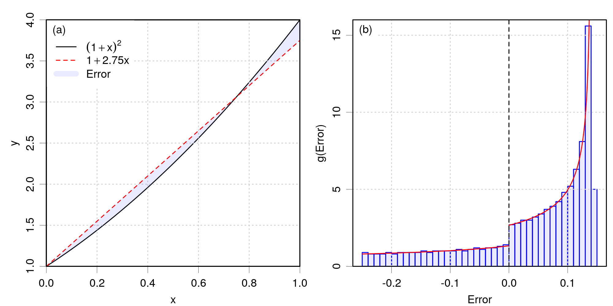
Figure 1: Model error distribution for the least-squares approximation of the curve $y=(1+x)^{2}$ by the linear model $\tilde{y}=1+2.75x$. (a) the curves and errors on $x\in[0,1]$; (b) the probability density of errors $g(Error)$ (red curve) and a histogram for a uniform sample of $x$.

Even if many error sets present distributions that are less symptomatic than the one shown here (see for instance those in Section III.1, Fig. 4), there is no reason to presume that they should be normally distributed. They could for instance present tails with a slow, sub-exponential, decay (so-called heavy tails) that prevent the reliable estimation of some common statistics.

II.2 Notations and definitions

II.2.1 Errors / signed errors

The calculated value $c_{i}$, for a system $i$ in a dataset of size $N$, differs from its reference value $r_{i}$ by an error

$$e_{i}=c_{i}-r_{i}$$ (4)

The formulae for the calculation of MUE and other statistics described below assume that the reference data and calculated values have no uncertainty, or uncertainties much smaller than the errors themselves. This is an ubiquitous assumption in the CC methods benchmarking literature. In the presence of non-negligible uncertainties with heterogeneous amplitudes, one should consider the use of weighted statistics Bevington and Robinson (1992).

Considering that the errors have a probability density function (PDF), noted $\pi(e)$, one defines the errors mean, $\mu$, standard deviation, $\sigma$, and cumulative distribution function (CDF), $G$, by

$$\mu =\int_{-\infty}^{\infty}x\,\pi(x)dx$$ (5)

$$\sigma =\int_{-\infty}^{\infty}(x-\mu)^{2}\pi(x)dx$$ (6)

$$G(\eta) =\int_{-\infty}^{\eta}\pi(x)\,dx$$ (7)

The CDF provides the probability that $e$ is smaller than a threshold $\eta$: $P(e\leq\eta)=G(\eta)$, where $P(X)$ is the probability of event $X$. Inversely, the value $\eta_{p}$ below which $e$ lies with probability $p=P(e\leq\eta_{p})$, is given by the inverse of the CDF (the quantile function), $\eta_{p}=G^{-1}(p)$.

Due to the finite size of the errors sample, one has only access to estimates of these properties, noted with a hat (e.g. $\hat{\mu}$)

$$\hat{\mu} \equiv MSE=\frac{1}{N}\sum_{i=1}^{N}e_{i}$$ (8)

$$\hat{\sigma} \equiv RMSD=\sqrt{\frac{1}{N-1}\sum_{i=1}^{N}(e_{i}-\hat{\mu})^{2}}$$ (9)

$$\hat{G}(\eta) =\frac{1}{N}\sum_{i=1}^{N}\mathbf{1}_{e_{i}\leq\eta}$$ (10)

where MSE is the mean signed error, RMSD is the root mean square deviation of errors, and $\mathbf{1}_{X}$ is the indicator function of event $X$. $\hat{G}(.)$ is called the empirical cumulative distribution function (ECDF).

II.2.2 Absolute / unsigned errors

The absolute values of errors, or unsigned errors, $\epsilon_{i}=\left|e_{i}\right|$, have a probability density function which results from the folding of $\pi(e)$ (Fig. 2 (a)) and is noted $\pi_{F}(\epsilon$). The mean, standard deviation of the folded distribution and its cumulative distribution function are

$$\mu_{F} =\int_{0}^{\infty}x\,\pi_{F}(x)dx$$ (11)

$$\sigma_{F} =\int_{0}^{\infty}(x-\mu_{F})^{2}\pi_{F}(x)dx$$ (12)

$$G_{F}(\eta) =\int_{0}^{\eta}\pi_{F}(x)\,dx$$ (13)

and they are estimated by

$$\hat{\mu}_{F} \equiv MUE=\frac{1}{N}\sum_{i=1}^{N}\epsilon_{i}$$ (14)

$$\hat{\sigma}_{F} =\sqrt{\frac{1}{N-1}\sum_{i=1}^{N}(\epsilon_{i}-\hat{\mu}_{F})^{2}}$$ (15)

$$\hat{G}_{F}(\eta) =\frac{1}{N}\sum_{i=1}^{N}\mathbf{1_{\epsilon_{i}\leq\eta}}$$ (16)

For simplicity, specific notations are used in the following for the cumulative probabilities and percentiles of the unsigned error distribution

$$C(\eta) =\hat{G}_{F}(\eta)$$ (17)

$$Q_{n} =\hat{G}_{F}^{-1}(n/100)$$ (18)

where $n$ is an integer between 0 and 100 and $n/100$ is the corresponding probability.

II.2.3 Statistical uncertainty of the estimators

Due to the limited size of the benchmark datasets one has to consider the statistical uncertainty (standard error) attached to the estimators presented above. The formulae given below are based on the asymptotic normality of the estimators distributions Stuart and Ord (1994). No strong assumption is done on the underlying error distribution, except for the uncertainty on the mean, where the standard deviation has to be finite. The formulae apply to both signed and unsigned errors by using the corresponding statistics, and are given here for unsigned errors:

• the standard error of a mean error is estimated by the usual formula

  $$u_{\hat{\mu}_{F}} =\frac{1}{\sqrt{N}}\hat{\sigma}_{F}$$ (19)

• the standard error of a cumulative probability $C(\eta)$ is given by Stuart and Ord (1994)

  $$u_{C(\eta)}=\sqrt{\frac{C(\eta)(1-C(\eta))}{N}}$$ (20)

• the standard error of a percentile $Q_{n}$ is estimated by Kendall’s formula Stuart and Ord (1994)

  $$u_{Q_{n}}=\frac{1}{100}\sqrt{\frac{n(100-n)}{N\,\pi_{F}^{2}(Q_{n})}}$$ (21)

  This formula is not well adapted for high percentiles (e.g., $n>80$), because the estimation of the unknown PDF $\pi_{F}(.)$ in this range is typically based on few sample points. We found it more reliable to estimate $u_{Q_{n}}$ and confidence intervals on $Q_{n}$ by bootstrapping Efron (1979) (Appendix A).

II.2.4 Remarks

The MSE is a location or centrality estimator, i.e., it is used to estimate the position of a representative value of the sample. As such, the MSE is helpful to detect biased error distributions (distributions for which the MSE is not small in comparison to the RMSD of the sample), and to modulate the interpretation of the MUE.

The MUE is particularly interesting as a robust dispersion statistics for residuals after model regression, i.e., when $|MSE|\ll MUE$, a scenario where it is much less sensitive to outliers than the root mean square of the residuals. However, this property is often lost when considering error distributions: in conditions where the MSE is not negligible before the MUE, the latter is no more a dispersion statistics Pernot et al. (2015). In the limit where the bias is very large, one gets $MUE\simeq\left|MSE\right|$, i.e. the MUE becomes a location statistics. Although the interpretation of the MUE is reputed to be “easy” Willmott and Matsuura (2005); Chai and Draxler (2014), it is difficult to analyze in non-ideal conditions. This crucial point is illustrated below, in Section II.3.

Note that for some heavy-tailed distributions (e.g., Cauchy, slash…) such statistics as the mean and/or the variance are not defined, but the CDF and quantiles are.

II.3 The Folded Normal Distribution

If $X$ is a normally distributed random variable with mean $\mu$ and standard deviation $\sigma$, $|X|$ has a folded normal distribution (FND) with PDF Leone, Nelson, and Nottingham (1961) (Fig. 2 (a))

$$\pi_{FN}(\epsilon;\mu,\sigma)=\frac{1}{\sqrt{2\pi\sigma^{2}}}\left[\exp\left(-\frac{\left(\epsilon-\mu\right)^{2}}{2\sigma^{2}}\right)+\exp\left(-\frac{\left(\epsilon+\mu\right)^{2}}{2\sigma^{2}}\right)\right]$$ (22)

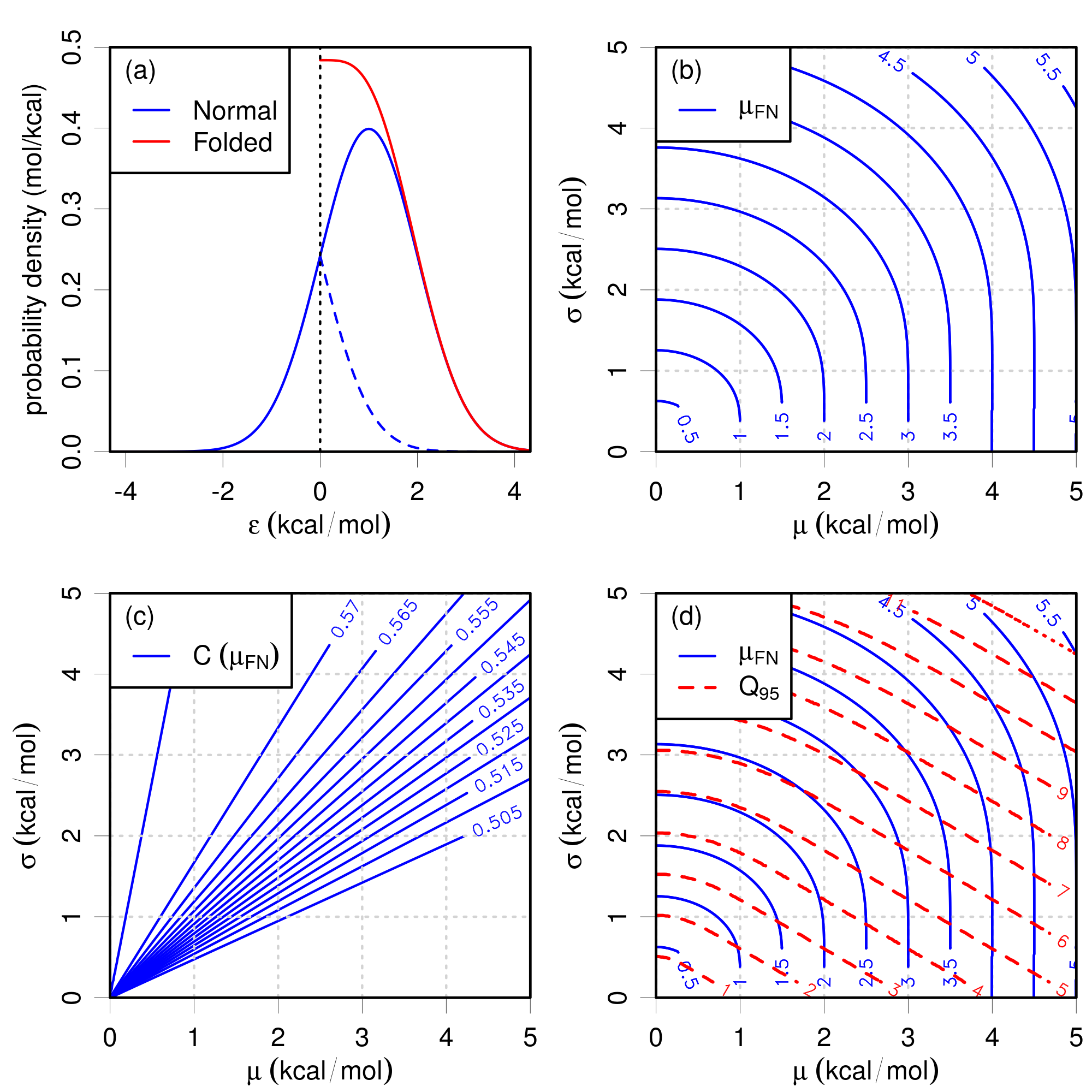
Figure 2: Construction of the folded normal distribution (FND) and relation of some of its properties with respect to the mean value ($\mu$) and standard deviation ($\sigma$) of the underlying normal distribution: (a) Construction: the negative tail of the normal distribution PDF (blue) is folded on the positive side (dashed), and addition to the positive error distribution yields the FND PDF (red); (b) Contour lines of $\mu_{FN}$, the mean of the FND, from Eq. 23; (c) Contour lines of the cumulative probability $C(\mu_{FN})$, corresponding to the values of $\mu_{FN}$ in panel (b); (d) Contour lines of the $95^{th}$ percentile of the FND, $Q_{95}$, superimposed on the contours of $\mu_{FN}$ reported from panel (b).

Mean value.

The mean $\mu_{FN}$ of the FND depends in a complex way on the parameters of the original normal distribution

$$\mu_{FN}(\mu,\sigma)=\sigma\sqrt{\frac{2}{\pi}}\exp\left(-\frac{\mu^{2}}{2\sigma^{2}}\right)-\mu\thinspace\mathrm{erf}\left(-\frac{\mu}{\sqrt{2}\sigma}\right),$$ (23)

so that a same value of $\mu_{FN}$ might result from very different normal distributions (e.g., small $\mu$ and large $\sigma$, large $\mu$ and small $\sigma$). The dependence of $\mu_{FN}$ on $(\mu,\sigma)$ is displayed by contour lines in Fig. 2 (b). Note that $\lim_{\sigma\rightarrow 0}(\mu_{FN})=\mu$.

Note also that a decrease of $\mu_{FN}$ can be achieved through a variety of paths in the $(\mu,\sigma)$ space, notably by decreasing $\mu$ and increasing $\sigma$, or vice versa. Therefore, in benchmarking studies, a lower MUE does not guarantee overall better performances, as shown in the following.

Cumulative probabilities.

The CDF, as the integral of $\pi_{FN}$, depends also on $\mu$ and $\sigma$

$$G_{FN}(\epsilon;\mu,\sigma)=\frac{1}{2}\left[\mathrm{erf}\left(\frac{\epsilon-\mu}{\sqrt{2}\sigma}\right)+\mathrm{erf}\left(\frac{\epsilon+\mu}{\sqrt{2}\sigma}\right)\right]$$ (24)

In order to investigate the interest of the MUE (exactly known here as $\mu_{FN}$) as a probabilistic estimator, one can calculate the corresponding cumulative probability

$$C(\mu_{FN})=P(\epsilon\leq\mu_{FN})=G_{FN}(\mu_{FN})$$ (25)

The value depends on $\mu$ and $\sigma$ (Fig. 2 (c)), and varies in the range $\left[0.5,0.5753\right]$. Even in ideal conditions of normal error distributions, there is not a unique cumulative probability attached to the MUE.

Percentiles.

Similarly, a chosen value of $\mu_{FN}$ corresponds to a wide range of values for the percentiles of the folded distribution (e.g., $Q_{95}$). In Fig. 2 (d), one can see that a single $\mu_{FN}$ contour line crosses several contour lines for $Q_{95}$. For instance, the $\mu_{FN}=2$ contour intersects with $Q_{95}$ lines varying in the $[2,5]$ kcal/mol range. This shows that in benchmarking studies, a small value of the MUE does not guarantee good predictive performance of a method.

However, a pair of values ($\mu_{FN},\mu$) might enable to determine a percentile uniquely. Using Fig. 2 (d), one can check, for instance, that the contour line for $\mu_{FN}=2.5$, intersects the vertical line for $\mu=2$ at a point where the value of $Q_{95}$ is about 6. This suggests that, at least for normal error distributions, the (MUE, MSE) pair provided by many benchmark studies might be used to infer probabilistic information on unsigned errors, in the same way as the (MSE, RMSD) pair would on signed errors. This will be tested in Section III.2.2.

II.4 Probabilistic estimators

We have shown above that model error distributions are not a priori normal, and that, even for normal error distributions, the MUE cannot provide unique probabilistic estimations. One is therefore in need of other kind of estimators to answer the questions posed in the introduction of this section. One needs in fact to be able to estimate probabilities associated with a chosen error level, and/or error levels associated with a chosen probability. The central tool for this kind of inquiry is the CDF. As we are interested mostly in the amplitude of errors, we will use the ECDF of unsigned errors $\hat{G}_{F}$ (Eq. 16).

In order to be more realistic than with the FND, we illustrate the following points on a concrete example: Fig. 3 shows the ECDF of the absolute errors on intensive atomization energies (IAE) by the B3LYP DFA. The definition of IAE is not relevant at this stage, and is presented in Section III.1. The shaded area delimits the 95% uncertainty band on the ECDF due to the sample size of the G3/99 dataset.

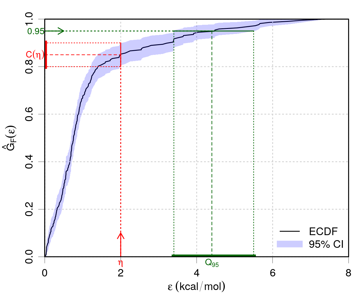
Figure 3: Empirical cumulative distribution function for B3LYP absolute errors on IAE for the G3/99 set. The shaded area delimits the 95% confidence interval on the ECDF. The colored lines provide examples of the inquiries that can be done from the ECDF (see text).

II.4.1 Probability of obtaining acceptable results

For the approach presented in this section, users have to decide what is an acceptable absolute error $\eta$ for their applications. Based on the data in the reference set, users can conclude whether their aim of getting acceptable results can be reached.

A trivial strategy would be to retain only methods for which $\max(\epsilon)<\eta$. Unfortunately, as most methods present large errors for some systems, this would hopelessly deplete the pool of usable methods. One has thus to accept some risk, and use a probabilistic criterion. The probability to obtain an acceptable absolute error level $\eta$ with a given method is estimated from the ECDF as $C(\eta)$ (Eq. 17).

As an illustration, consider Fig. 3: if one chooses an acceptance threshold for errors on IAE of $\eta=2$ kcal/mol (red arrow), one gets $C(2)\simeq 0.85$. Considering the statistical uncertainty on the ECDF one has indeed between 80 and 90 percent chances to achieve this maximum error level with B3LYP. So, out of 10 calculations for new systems with this DFA, one should expect that, on average, only 1 or 2 will provide IAE results with errors exceeding the chosen limit of 2 kcal/mol.

II.4.2 High confidence error level

Instead of obtaining the probability $C(\eta)$ after specifying the reliability parameter $\eta$, one may decide on a required confidence level about the outcome of a calculation and check the corresponding error level. One specifies thus first a probability of success (e.g., $p=$0.90 or 0.95), and then search the largest absolute error $\epsilon$ one has to accept, so that this probability level can be reached. Here again, the answer is given by the ECDF, through its inverse function and the percentiles $Q_{n}$, with $n=100\times p$ (Eq. 18).

For instance, using the ECDF for B3LYP (Fig. 3), the IAE absolute error corresponding to a 0.95 probability level is $Q_{95}\simeq 4.4$ kcal/mol. Considering the uncertainty on the ECDF, the error level to accept lies between 3.4 and 5.5 kcal/mol.

The risk level associated with the choice of a high-probability percentile can also be stated in terms of the percentage of new calculations for which the absolute errors are expected to exceed the chosen percentile. For $Q_{n},$ this number is on average $(100-n)$ %. For a new molecule with similar properties to the ones in the reference dataset, one has on average only 5 % chance to exceed the $Q_{95}$ error level. Of course, there is a distribution of excess chances, which depends on the size of the reference dataset and on the probability level.

For the choice of a success/risk level, one has to appreciate that, due to the errors sample size, the uncertainty on the percentiles increases with the probability. For B3LYP for instance, the upper bound of a 95% confidence interval (CI) on $Q_{95}$, noted $\left\lceil Q_{95}\right\rceil$, is about 5.5 kcal/mol (Table 2). If one is ready to accept a 10 % risk, the values are somewhat smaller, with $Q_{90}=3.2$ and $\left\lceil Q_{90}\right\rceil=3.9$ kcal/mol. The choice of a success/risk level has therefore to be guided by several considerations:

• For small reference datasets, the uncertainty on high percentiles might be large (Appendix A), and it might be pointless to discern $Q_{90}$ from $Q_{95}$. This would be the case for datasets with less than 100 points. In the present study case, with more than 200 points, their 95 % confidence intervals still overlap (see also Table 2), but the median value of one percentile lies outside of the 95 % CI of the other.

• It is also noteworthy that higher quantiles might be more influenced by outliers. However, a level of 10 % or even 5 % of outliers in a dataset starts to be problematic anyway, and they should be treated before performing statistical estimation.

• Some heavily corrected methods, such as the composite methods for thermochemistry, lead to quasi-normal error distributions Klippenstein, Harding, and Ruscic (2017). In such cases, it has been recommended by Ruscic Ruscic (2014) to use an enlarged uncertainty $u_{95\%}$ to summarize the errors. Using an enlarged uncertainty assumes the symmetry of the error distribution, not its normality, and provides probabilistic information on the performance of the method BIPM et al. (2008): $P(\hat{\mu}-u_{95\%}\leq e\leq\hat{\mu}+u_{95\%})=0.95$. In the case of unbiased methods ($\hat{\mu}\simeq 0$) this translates for unsigned errors as $P(\epsilon\leq u_{95\%})=0.95$, which is the definition of $Q_{95}$ (Eq. 18). Therefore, by using $Q_{95}$ as a probabilistic estimator in the case of general error distributions, one ensures a direct link to the recommended usage for symmetric distributions.

III Application

III.1 Exploring the data sets

To illustrate the concepts developed in this article, we consider the errors on the atomization energies (AE) of the G3/99 database Curtiss et al. (2000). We base our study on published data Otero-de-la Roza and Johnson (2013), produced with the following DFAs: PW86PBE Perdew and Yue (1986); Perdew, Burke, and Ernzerhof (1996), B3LYP Lee, Yang, and Parr (1988); Becke (1993), PBE0 Adamo and Barone (1999), CAM-B3LYP Yanai, Tew, and Handy (2004), LC-$\omega$PBE Vydrov and Scuseria (2006); Vydrov et al. (2006), PBE Perdew, Burke, and Ernzerhof (1996), BLYP Becke (1988); Lee, Yang, and Parr (1988), BH&HLYP Becke (1993), and B97-1 Hamprecht et al. (1998). BLYP, PBE and PW86PBE are pure functionals, the remaining are hybrids, CAM-B3LYP and LC-$\omega$PBE using range-separation.

Due to the extensivity of the atomization energies, it has been shown that errors typically increase with the size of the system Savin and Johnson (2015); Perdew et al. (2016); Margraf, Ranasinghe, and Bartlett (2017). To eliminate this trend, we also consider the atomization energies per atom, noted IAE for intensive atomization energies Perdew et al. (2016).

III.1.1 Benchmarking statistics

First, we report reference statistics as found in most CC methods benchmarking studies (Table 1), namely, the MUE, MSE, RMSD, Lowest Negative Error (LNE) and Highest Positive Error (HPE). We omit the root mean squared error (RMSE, mean of the uncentered errors) which is often reported alongside the MUE, but has no practical interest here, and include instead the RMSD, which is useful to assess the importance of the bias. See Section II.2 for definitions of these statistics.

Table 1: Statistics of AE and IAE errors on the G3/99 dataset for a selection of DFAs. MUE: mean unsigned error; MSE: mean signed error; RMSD: root mean square deviation; LNE: lowest negative error; HPE: highest positive error.

DFA	Error Statistics for AE (kcal/mol)											Error Statistics for IAE (kcal/mol)
	MUE		MSE		RMSD		LNE		HPE			MUE		MSE		RMSD		LNE		HPE
B3LYP	7.	8	7.	2	7.	9	-7.	8	39.	5		1.	2	1.	0	1.	5	-3.	9	7.	4
B97-1	6.	1	4.	8	6.	8	-9.	3	24.	7		0.	9	0.	5	1.	1	-3.	2	4.	6
BH&HLYP	32.	3	32.	2	18.	5	-7.	4	83.	4		4.	8	4.	8	3.	5	-3.	7	20.	5
BLYP	11.	4	7.	5	12.	9	-25.	4	45.	3		1.	6	0.	4	2.	2	-8.	5	7.	0
CAM-B3LYP	4.	2	2.	3	6.	6	-7.	8	32.	7		0.	9	0.	6	1.	5	-3.	9	6.	8
LC-$\omega$PBE	5.	1	2.	9	6.	4	-14.	0	27.	3		1.	1	0.	7	1.	7	-3.	6	9.	5
PBE	18.	9	-17.	9	15.	5	-75.	0	14.	0		2.	8	-2.	5	2.	7	-13.	6	2.	8
PBE0	5.	5	-1.	0	8.	2	-31.	1	29.	3		0.	9	0.	2	1.	4	-2.	9	6.	5
PW86PBE	9.	4	-1.	5	12.	2	-33.	8	29.	8		1.	6	-0.	5	2.	5	-11.	3	5.	9

Considering AE, the DFA with the smallest MUE is CAM-B3LYP (4.2 kcal/mol). It has a noticeable bias (MSE) of about 2.3 kcal/mol, to be compared to a RMSD of 6.6 kcal/mol. The errors are dispersed in a range |HPE-LNE| of about 40 kcal/mol. The DFA with the smallest error range in the set is B97-1 (34 kcal/mol), but it is more strongly biased than CAM-B3LYP (4.8 kcal/mol) and has a larger MUE (6.1 kcal/mol).

For intensive atomization energies, three DFAs share the lowest MUE of 0.9 kcal/mol (B97-1, CAM-B3LYP and PBE0). Among those, PBE0 is the least biased, but B97-1 has the smallest error range. However, one should keep in mind that the error range might reflect the presence of outliers, and not characterize properly the properties of the error distribution.

So, which DFA is the best, in the sense that it minimizes the risk to get a large error when predicting the AE or IAE of a new system? It is difficult to conclude from these statistics, and additional information is clearly needed: one has to go beyond elementary summary statistics and consider the underlying error distributions.

III.1.2 Error distributions in the G3/99 AE and IAE sets

Assuming that the level of uncertainty in the reference data is negligible (less than 1 kcal/mol on formation enthalpies according to Curtiss et al. Curtiss et al. (2000)), and that the numerical errors in the calculated data are assumed to be well controlled Irikura, Johnson, and Kacker (2004), discrepancy between calculated and reference values in the present dataset reflects either systematic errors from the DFA (modeling and discretization errors) or improper reference data Pernot et al. (2015).

Fig. 4 shows histograms of the B3LYP errors. A normal distribution having the same mean and standard deviation as the errors set has been overlaid on the histogram. At a first glance, one notices that the normal distribution does not faithfully describe the distribution of errors. The latter has a more pronounced peak slightly right of the origin, and presents some asymmetry: positive errors, even very large ones, occur more often than negative ones. The deviation towards positive errors explains why the normal distribution does not have its center on the sharp peak, and also is broader than this peak.

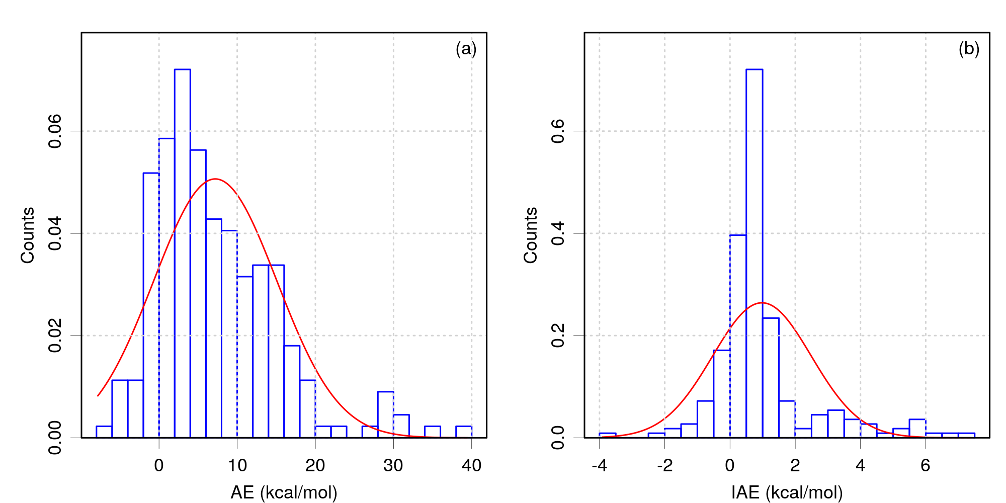
Figure 4: Histograms of the B3LYP errors for AE in the G3/99 set. A normal probability density function having the same mean and standard deviation is superimposed. (a) atomization energies ($\mu=$7.2 kcal/mol, $\sigma=$7.9 kcal/mol); (b) intensive atomization energies ($\mu=$1.0 kcal/mol, $\sigma=$1.5 kcal/mol).

Note that the non-normality observed on the histograms might also be an effect of the limited size of the sample. Some numbers below suggest, however, that this cannot be the only cause of discrepancy: the sampling errors seem to be systematically lower than the discrepancies one sees in Fig. 4. One is therefore in need of statistics that convey useful information on non-normal distributions.

III.1.3 Histograms do not tell the whole story

Histograms themselves are summaries that can hide important features in the errors set. It is generally rewarding to analyze the errors sample for underlying features, such as systems classes to be treated separately Faver et al. (2011). Even histograms with a single maximum (mode) can hide some heterogeneity in the sample. A very useful graphical representation to reveal such features is to plot the errors as a function of the calculated or reference property, as in Fig. 5, which displays side-by-side a scatterplot and the corresponding histogram. The latter results from the projection and binning of the data cloud on the ordinates axis: trends and heterogeneity in the data cloud contribute to features in the histogram (asymmetry, multimodality, …).

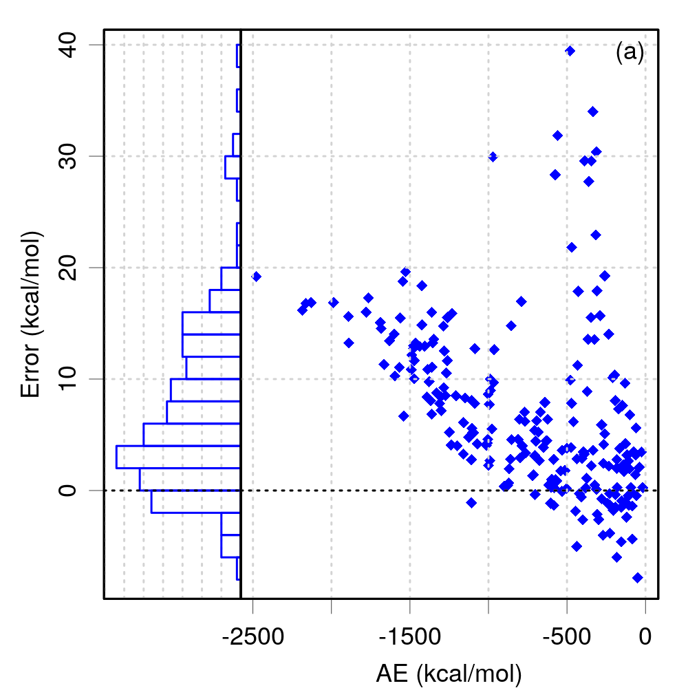
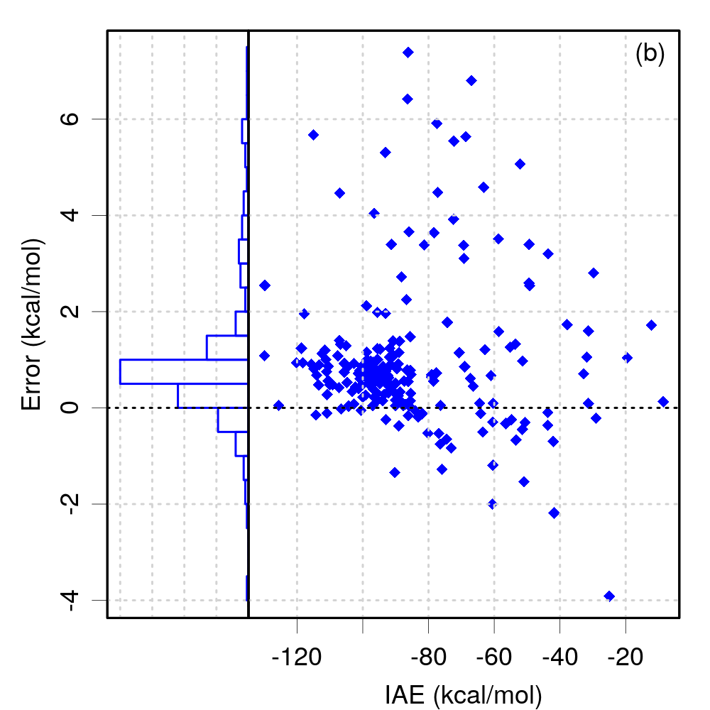
Figure 5: Distributions of the B3LYP errors for AE and IAE in the G3/99 set. Errors are plotted as a function of the reference data. Histograms of the errors sets are plotted for comparison: (a) atomization energies; (b) intensive atomization energies.

In the B3LYP case, one sees immediately that there are two problems: (i) two branches in the dataset, with different trends, and (ii) a strong (linear) dependence of the main set of errors with the atomization energy. The upper, almost vertical, branch can be exclusively assigned to molecules containing atoms out of the CHON set. The main, lower, branch contains mostly CHON-type molecules, but also some non-CHON systems. The linear trend in the main branch is linked to the extensivity of atomization energies. This can be checked by plotting the errors as a function of the number of atoms in the molecule (Fig. 6, top left). The monotonous increase of the main branch with the number of atoms is clear, whereas the effect is less marked for the non-CHON branch. From this simple analysis, one sees that the prediction error for an AE calculation with B3LYP will depend (1) on the nature of the molecule, and (2) on its size.

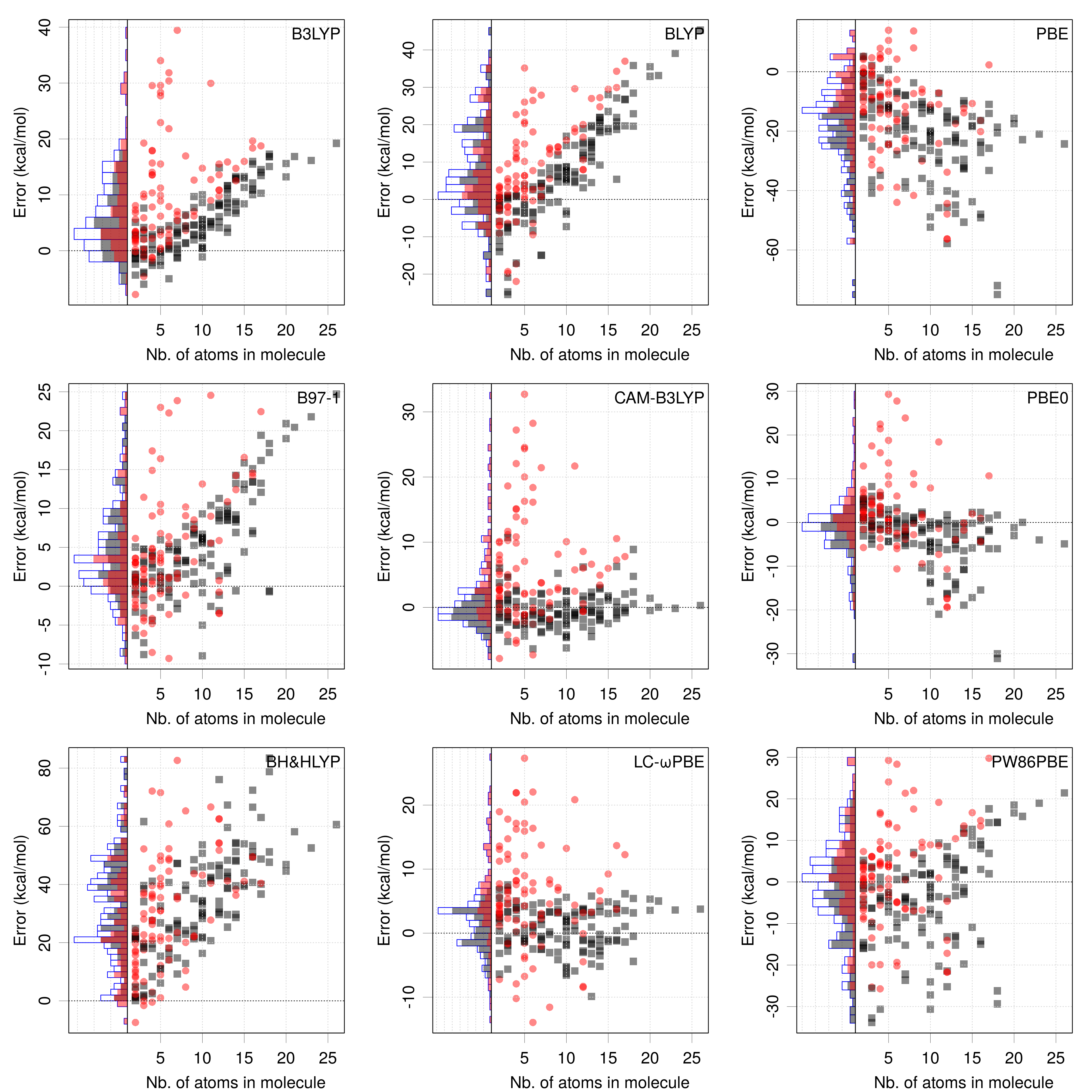
Figure 6: Distribution of the errors for AE as a function of the number of atoms in the molecules of the G3/99 set for nine DFAs. The data points are coded for CHON-type molecules (gray squares and histogram) and the other ones (red circles and histogram). The histograms corresponding to the partial and whole datasets are displayed in the left panel of each graph. The histogram for the whole dataset is traced with blue lines.

Considering the error distribution for the other DFAs in Fig. 6, different cases are observed: the linear increase of the AE errors with the number of atoms is also observed for BLYP, BH&HLYP and B97-1, whereas CAM-B3LYP and LC-$\omega$PBE errors are mostly independent of the molecule size, and an overall decrease is observed for PBE and PBE0. The heterogeneity of non-CHON systems is mostly observed for B3LYP, CAM-B3LYP, LC-$\omega$PBE, PBE0 and B97-1, whereas PBE, PW86PBE and BH&HLYP errors seem mostly uncorrelated with the chemical composition.

To achieve the most accurate results for some DFAs, it would be desirable to split the G3/99 set and perform statistics on the separate subsets. However, for the sake of simplicity and fairness with regard to other DFAs, we will continue here to work with the full G3/99 test set, without questioning its homogeneity.

The use of IAE solves in a large part the size-dependence problem of AE (Fig. 7), but one is left with the composition heterogeneity problem for some DFAs. Note that even for IAE, most error distributions are neither normal, nor zero-centered (e.g., B3LYP, PBE, BLYP, BH&HLYP, B97-1).

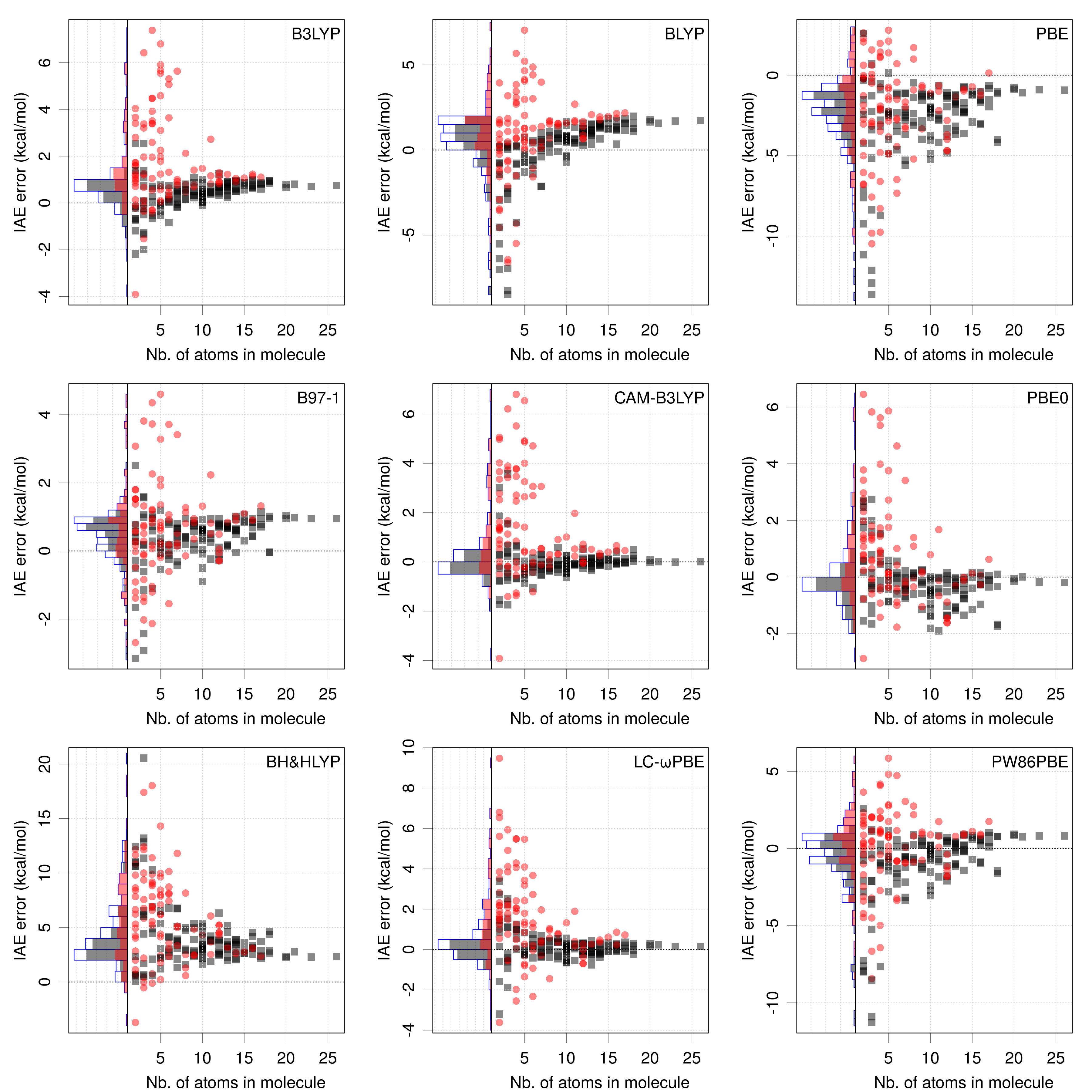
Figure 7: Same as Fig. 6 for IAE.

III.1.4 Searching for outliers

Points lying far in the wings of the histograms of error sets might suggest inconsistent data in the reference set. Considering the linear trends in the AE errors for several DFAs, extreme points might rather be due to the molecule size than to a data problem. It is therefore best to use IAE to identify outliers Perdew et al. (2016). Outliers have been tagged here as systems having IAE errors outside of the 95 % signed error range for a given DFA. The most common outliers in the present DFA set are NO₂ (7/9 DFAs), SO₂, SiF₄, N₂O, SO₃, O₂ (6/9 DFAs) and BeH (5/9 DFAs). Some of these outliers have already been identified by Perdew et al. Perdew et al. (2016), who discuss them with regard to the DFAs properties.

An important observation is that no outlier is common to all DFAs (Fig. 8), which indicates that the observed extreme values are essentially due to limitations of the models, not to abnormal reference data. There is therefore no solid reason to prune the dataset in order improve the normality of the error distributions. As stated above, one has definitely to deal with non-normal distributions and adopt informative statistics enabling final users to make their choice of DFA.

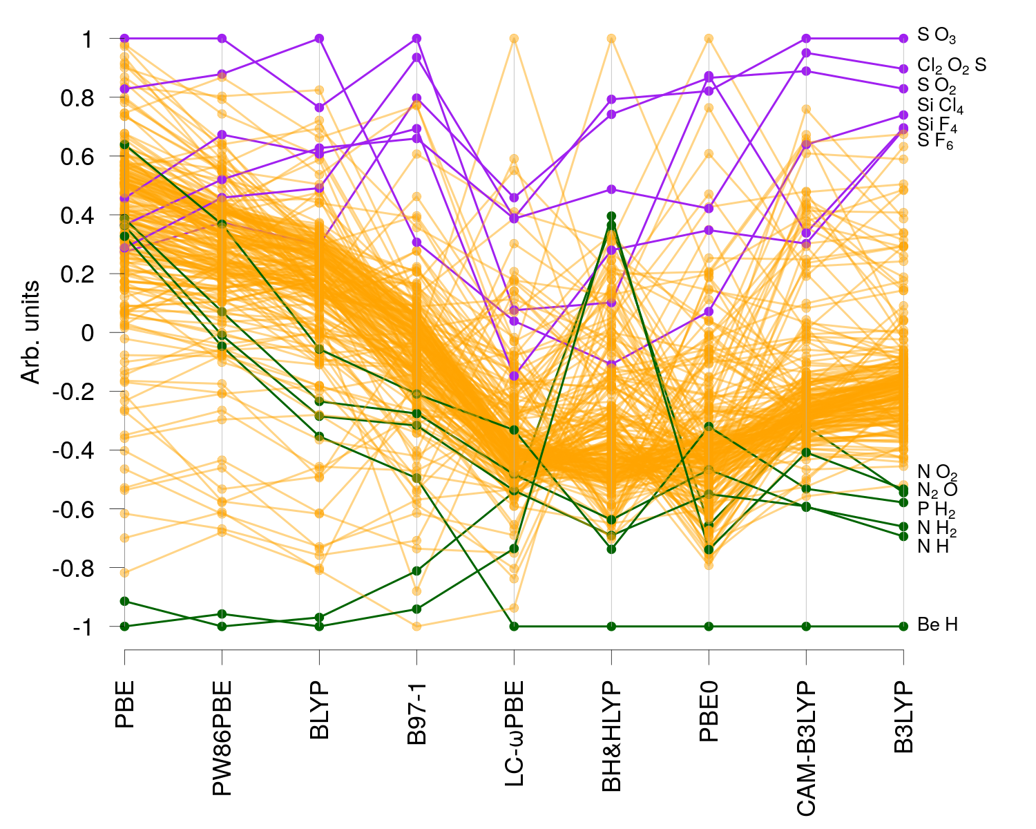
Figure 8: Parallel plot of the IAE errors in the G3/99 dataset. All error sets have been linearly rescaled to a common $\left[-1,1\right]$ range. Lines join identical molecules in each set. The DFAs have been ordered to display similarity in outliers patterns. The labels on the right show selected outliers for B3LYP.

III.1.5 Summary

A useful tool to reveal features in the error sets is to plot the errors as a function of the calculated or reference values, or any other relevant property. Histograms contain more information than summary statistics, but they do not tell the whole story!

From the exploration of the G3/99 dataset for AE and IAE, one might underline that the error distributions are complex and structured by several properties, such as the chemical composition (CHON vs. non-CHON) and the size of the molecule. Moreover, in these error sets, the non-normality of the distributions is the rule rather than the exception, which implies that the usual summary statistics are not sufficient to enable reliable error predictions. This justifies the need to turn to statistical tools not currently used in the CC methods benchmarking literature, such as the cumulative probabilities and percentiles presented in Section II.

Considering the size-dependence of AE errors for most DFAs in our set (Fig. 6), it is worthless to design simple and reliable probabilistic indicators for this property. For instance, B3LYP calculation for CHON molecules with more than 40 atoms will present errors exceeding those present in the G3/99 set. In consequence, only IAE error sets will be considered in the following.

III.2 Probabilistic estimators for unsigned errors

In this section, we analyze the probabilistic estimators for unsigned errors. Working on unsigned errors implies to accept a loss of information to concentrate on the amplitude of errors. Note that probabilistic estimators could as well be designed for signed errors, for instance a pair of 2.5% and 97.5% quantiles delimiting a 95 % probability interval, but they would lead to more complex ranking procedures.

III.2.1 Statistics of unsigned errors and their uncertainty

Statistics of unsigned IAE errors and their uncertainty have been computed for all DFAs listed above: MUE, cumulative probability for several thresholds, and a set of percentiles and limits of 95 % CI for the higher percentiles. The uncertainties are reported in the parenthetical notation, where “the number in parentheses is the numerical value of the standard uncertainty referred to the corresponding last digits of the quoted result” BIPM et al. (2008). The percentiles uncertainty and CI limits have been calculated by bootstrapping, with 1000 repetitions (Appendix A). The results are presented in Table 2. The corresponding ECDFs are shown in Fig. 9, with the $Q_{95}$ percentile and its 95 % CI. Besides, these curves enable to estimate $C(\epsilon)$ and $Q_{n}$ at any level.

Table 2: Statistics for the unsigned errors of IAE for the G3/99 dataset. The lower and upper limits of 95 % confidence intervals on the $Q_{90}$and $Q_{95}$ percentiles are notes as floor ($\left\lfloor x\right\rfloor$) and ceiling ($\left\lceil x\right\rceil$), respectively. The optimal value in each column is noted by bold characters.

DFA	$MUE$		$C(MUE)$		$C(0.25)$		$C(0.5)$	$C(1.0)$	$C(2.0)$
B3LYP	1.	2(1)	0.	73(3)	0.	15(2)	0.29(3)	0.68(3)	0.	86(2)
B97-1	0.	85(5)	0.	64(3)	0.	20(3)	0.35(3)	0.75(3)	0.	92(2)
BH&HLYP	4.	8(2)	0.	64(3)	0.	018(9)	0.02(1)	0.07(2)	0.	12(2)
BLYP	1.	6(1)	0.	70(3)	0.	08(2)	0.19(3)	0.41(3)	0.	79(3)
CAM-B3LYP	0.	90(9)	0.	76(3)	0.	41(3)	0.62(3)	0.76(3)	0.	86(2)
LC-$\omega$PBE	1.	1(1)	0.	69(3)	0.	30(3)	0.51(3)	0.69(3)	0.	82(3)
PBE	2.	8(2)	0.	63(3)	0.	04(1)	0.06(2)	0.18(3)	0.	45(3)
PBE0	0.	92(8)	0.	66(3)	0.	30(3)	0.49(3)	0.68(3)	0.	90(2)
PW86PBE	1.	6(1)	0.	69(3)	0.	13(2)	0.24(3)	0.55(3)	0.	75(3)
DFA	$Q_{50}$		$Q_{75}$		$Q_{90}$		$\left\lfloor Q_{90}\right\rfloor,\left\lceil Q_{90}\right\rceil$		$Q_{95}$		$\left\lfloor Q_{95}\right\rfloor,\left\lceil Q_{95}\right\rceil$
B3LYP	0.	80(4)	1.	2(1)	3.	2(5)	2.0, 3.9		4.	4(6)	3.4, 5.5
B97-1	0.	70(4)	1.	0(1)	1.	6(2)	1.4, 2.1		2.	5(4)	1.8, 3.3
BH&HLYP	3.	8(2)	6.	3(5)	10.	0(7)	8.4, 11.0		11.	6(6)	10.3, 12.4
BLYP	1.	3(1)	1.	8(1)	3.	9(5)	2.9, 4.6		5.	2(6)	4.3, 6.4
CAM-B3LYP	0.	30(5)	0.	9(2)	3.	1(4)	1.9, 3.8		3.	9(4)	3.4, 4.9
LC-$\omega$PBE	0.	5(1)	1.	4(2)	2.	8(4)	2.2, 3.8		4.	1(6)	3.4, 5.5
PBE	2.	2(1)	3.	5(3)	5.	3(7)	4.8, 7.1		7.	6(9)	6.4, 9.8
PBE0	0.	5(1)	1.	3(1)	2.	0(3)	1.7, 2.7		3.	0(5)	2.5, 4.0
PW86PBE	0.	9(1)	2.	0(2)	3.	6(5)	2.8, 4.8		5.	8(1)	4.2, 7.7

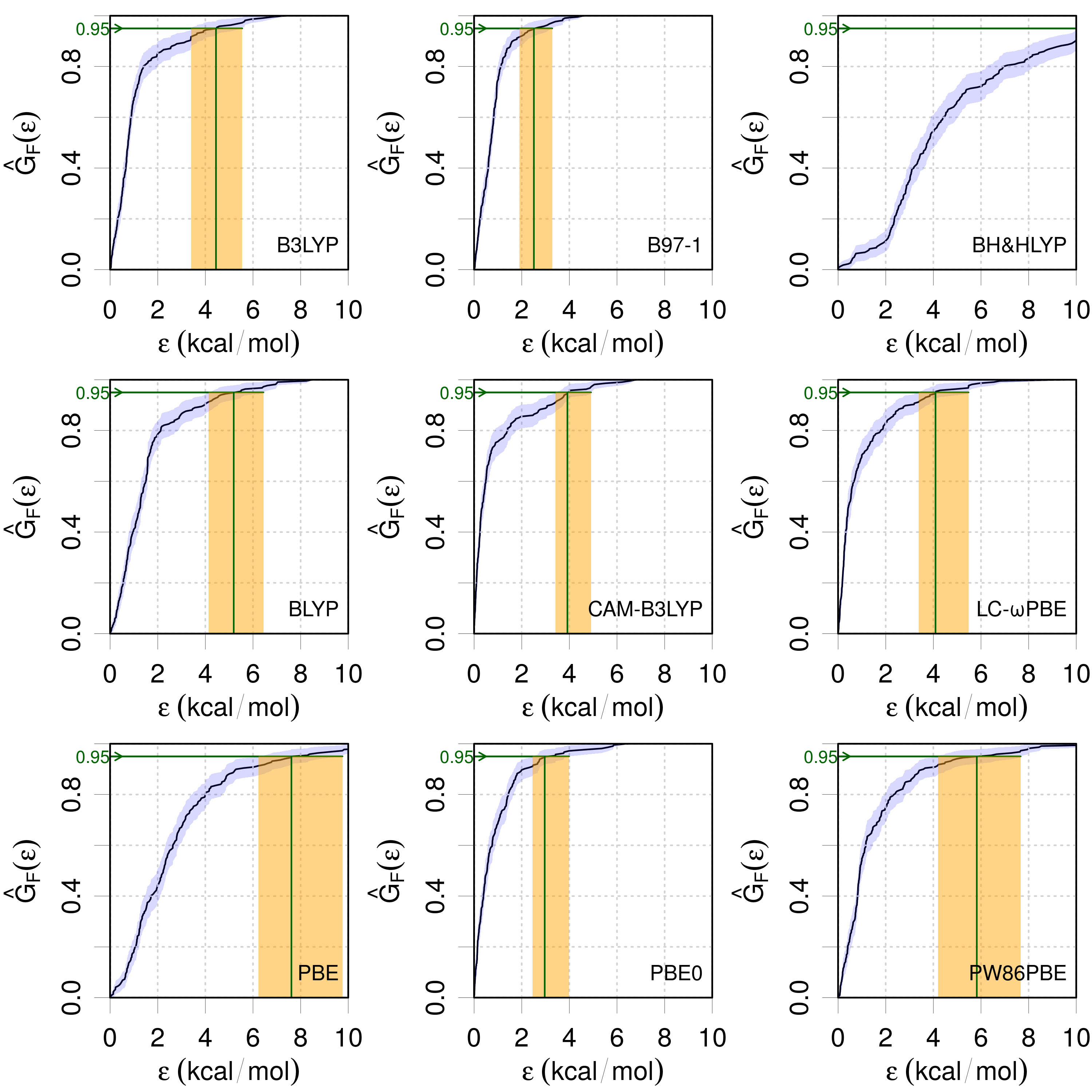
Figure 9: Empirical cumulative distribution function for unsigned errors on IAE, based on calculations for the G3/99 set. The shaded area delimits the 95% uncertainty band on the ECDF. The $Q_{95}$ percentile is indicated by a vertical green line, and the orange area delimits its 95 % CI.

If one considers the cumulative probabilities, several points are outstanding. $C(\eta)$ for small values of $\eta$ (below the “chemical accuracy” of 1 kcal/mol) are small for all DFAs, with a maximum of 0.76(3) for CAM-B3LYP at $\eta=1$ kcal/mol. Imposing smaller error limits means accepting less reliable predictions. If one increases the acceptance threshold to $\eta=2$ kcal/mol, one reaches reasonable confidence levels of 0.92(3) for B97-1 and 0.90(3) for PBE0. To achieve the widely used confidence limit of 95 %, one has to accept higher IAE error levels, for instance 3.9 kcal/mol for CAM-B3LYP (cf. $Q_{95}$ values in Table 2).

The fact that, in order to make a statement that is valid with high probability one has to accept large errors, is not conveyed by the MUE. The latter might induce us to think that a typical IAE error level for methods such as B97-1, CAM-B3LYP and PBE0 is around 1 kcal/mol. In fact, the cumulative probabilities at the MUE ($C(MUE)$ in Table 2) range between 0.63(3) and 0.76(3). Note that this is higher than the upper limit of 0.5753 estimated for the FND (Section II.3; Fig. 11 (a)), but still low in terms of prediction confidence. In consequence, the risk for the user to get absolute errors exceeding the MUE is unpredictable from the MUE alone and rather high (up to 40 %). This disqualifies the MUE as a basis for probabilistic estimations.

Looking at $Q_{95}$ one can see that three methods having similar MUEs (B97-1, CAM-B3LYP and PBE0) can have significantly different values of this high probability percentile, ranging from 2.5(4) for B97-1 to 3.9(4) kcal/mol for CAM-B3LYP. This raises the interest of $Q_{95}$ as a ranking metric, as reported below.

III.2.2 Estimation of percentiles from MUE and MSE

We have shown in Section II.3 that, in the ideal case of a normal error distribution, it is possible to estimate percentiles of the corresponding folded distribution from MSE ($\hat{\mu}$) and MUE ($\hat{\mu}_{F}$). This property is tested here on more realistic error distributions. $Q_{95F}$ has been estimated from the MUE and MSE, following the procedure described in Section II.3. A 95 % CI has been obtained by bootstrapping. Fig. 10 compares $Q_{95F}$ and $Q_{95}$. Considering the position of the points and the absence of intersection of the error bars with the identity line, one can conclude that $Q_{95F}$ significantly underestimates $Q_{95}$, except for B97-1, where the uncertainty on $Q_{95}$ is large enough to leave a doubt. Due to the non-normality of the error distributions, one cannot reliably estimate $Q_{n}$ from the generally available MSE and MUE statistics.

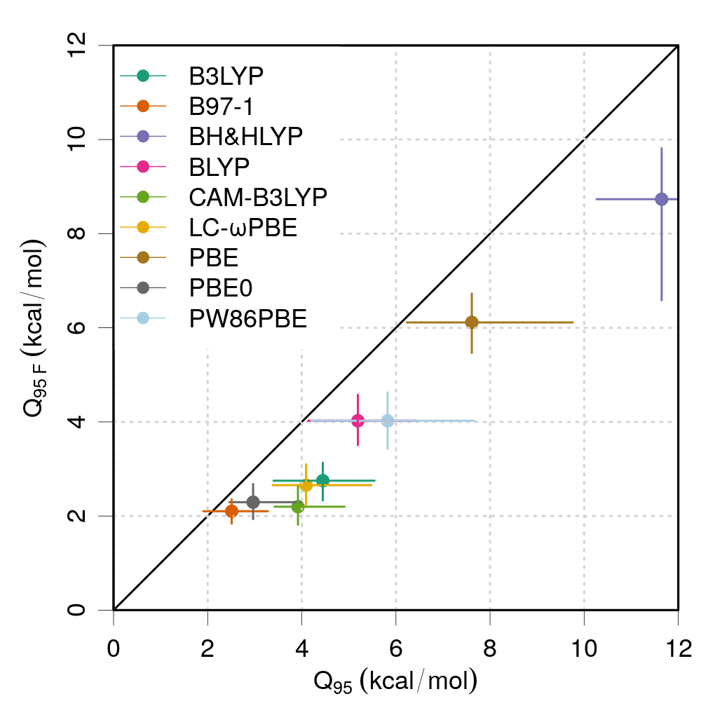
Figure 10: Comparison of $Q_{95}$ and its approximation $Q_{95F}$. The error bars represent 95 % confidence intervals.

III.3 DFA ranking

Table 3: Inversion probabilities in the MUE ranking. These give the probability (as percentage) that a row DFA achieves a lower MUE than a column DFAs with smaller mean MUE value because of sampling uncertainty. The DFAs are ordered by increasing mean MUE. Bold type indicates values higher than 20 %.

	B97-1	CAM-B3LYP	PBE0	LC-$\omega$PBE	B3LYP	BLYP	PW86PBE	PBE
B97-1
CAM-B3LYP	44
PBE0	40	47
LC-$\omega$PBE	23	28	30
B3LYP	14	19	20	39
BLYP	1	2	2	6	9
PW86PBE	2	2	3	7	11	49
PBE	0	0	0	0	0	0	0
BH&HLYP	0	0	0	0	0	0	0	0

III.3.1 Impact of statistical uncertainty on MUE-based ranking

When ranking DFAs by their MUE, the sampling uncertainty on the statistic has ideally to be taken into account, which, to our knowledge, is never reported in the literature.

Considering the MUE for two DFAs, $MUE_{1}$ and $MUE_{2}$ with mean values and standard errors $\mu_{F1}\pm u_{1}$ and $\mu_{F2}\pm u_{2}$ (Eq. 19), the probability density function of $MUE_{1}-MUE_{2}$ is a normal PDF with mean $\mu=\mu_{F1}-\mu_{F2}$ and variance $\sigma^{2}=u_{1}^{2}+u_{2}^{2}$. Therefore, one gets $P(MUE_{1}-MUE_{2}<0)$ as the cumulative probability

$$P(MUE_{1}<MUE_{2})\simeq\Phi(0,\mu=\mu_{F1}-\mu_{F2},\sigma^{2}=u_{1}^{2}+u_{2}^{2})$$ (26)

where $\Phi(x;\mu,\sigma^{2})$ is the cumulative distribution function for a normal distribution with mean $\mu$ and variance $\sigma^{2}$ (cf. Section II.2.3). Using Eq. 26, an ordering inversion probability has been evaluated for pairs of DFAs with $\mu_{F1}>\mu_{F2}$, and reported in Table 3. Note that this configuration implies that the upper limit of the inversion probability is $0.5$.

There is a neat segregation of the DFAs in two groups: (1) B97-1, CAM-B3LYP, PBE0, LC-$\omega$PBE and B3LYP, among which the inversion risk is medium to very high; and (2) BLYP, PW86PBE, PBE and BH&HLYP, which have vanishing chances to outperform any DFA of the first group. In the second group, the MUE ranking of PW86PBE and BLYP is not statistically significant.

III.3.2 Ranking by percentiles

As we have ruled out the use of MUE for probabilistic estimation, could it also be replaced for DFA ranking? Ranking of approximations could be done according to the values of $C(\epsilon)$ for a given $\epsilon$: the higher $C(\epsilon)$ the better the method. Alternatively, one can rank approximations by choosing a percentile $Q_{n}$: the lower $Q_{n}$, the better the method. As one can more easily and generally agree on a reference percentile than on an error level, the former being independent on the type of analyzed property, we test here how high-probability percentiles such as $Q_{95}$ can be used for the ranking of DFAs, and how they compare to MUE-based ranking.

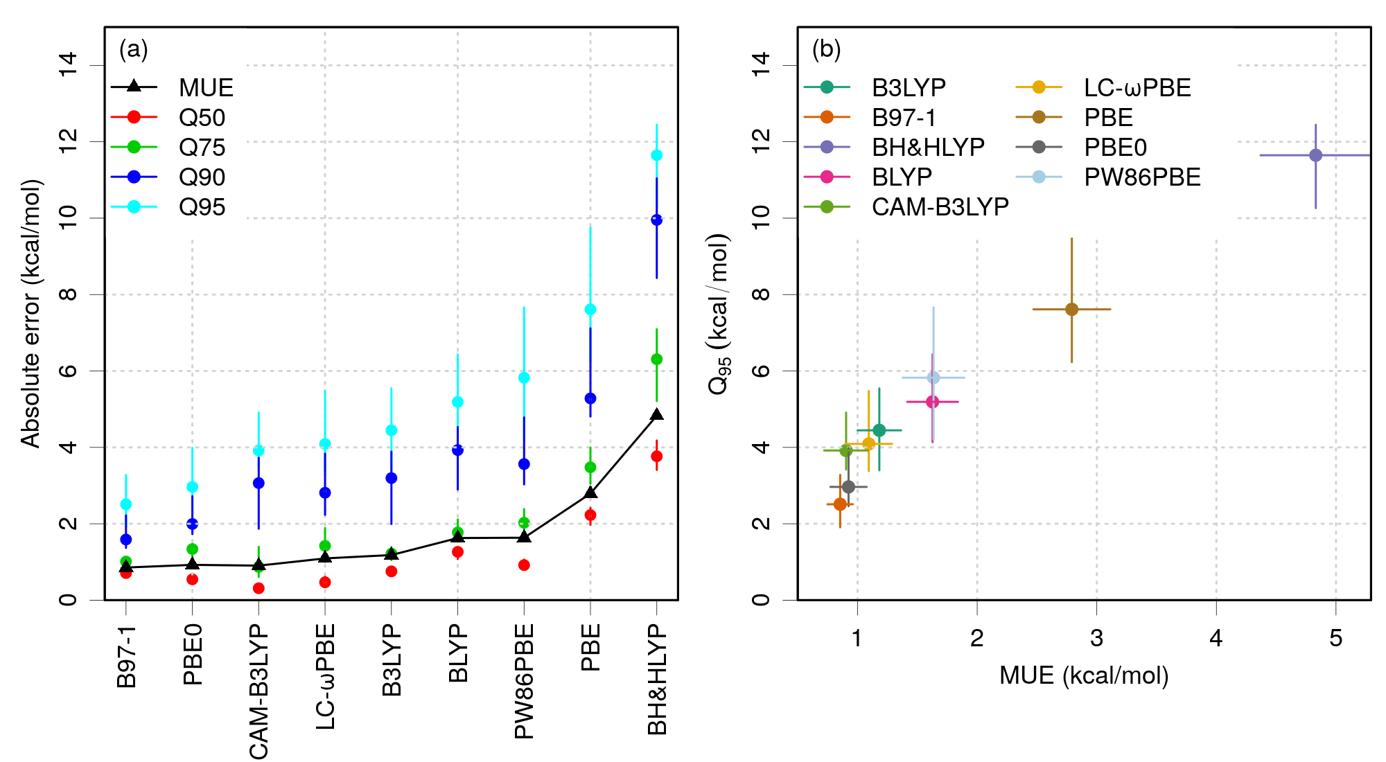
Figure 11: Comparison of statistics for ranking. (a) $MUE$ and $Q_{50}$, $Q_{75}$, $Q_{90}$ ,$Q_{95}$ percentiles for the set of DFAs, sorted by increasing value of $Q_{95}$; (b) correlation between MUE and $Q_{95}$. The error bars represent 95 % confidence intervals.

In order to facilitate the comparison between methods, the percentiles in Table 2 have been plotted together in Fig. 11(a), along with the MUE, and sorted by increasing $Q_{95}$ values. One sees that CAM-B3LYP is best at the 50 % level, but is challenged by B97-1 at the 75 % level and then by PBE0 at higher probability levels. As noted above, CAM-B3LYP, B97-1 and PBE0 have the same $MUE$ for this property ($\sim 0.9(1)$). The high percentiles can thus provide additional discriminating ranking criteria. Note that it is not surprising that, as a rule, hybrid methods (with the notable exception of the pioneering BH&HLYP) come out better than pure functionals.

Globally, if one compares the ranking by $MUE$ and $Q_{95}$ (Fig. 11(b)), the correlation is strong, except for the CAM-B3LYP/PBE0 inversion, which is not statistically significant, considering the high inversion probability estimated from the MUE standard errors (Table 3). The consideration of the error bars on the statistics shows that a strict ranking by the mean value of the statistics is not pertinent here. The definition of groups of methods would be more statistically relevant.

So, it appears that $Q_{95}$, beyond its added value for prediction errors estimation, would also be a relevant substitute to $MUE$ for the ranking of DFAs, or any computational chemistry methods. On the present dataset, it does not profoundly scramble the usual ranking, which is a reassuring point for its introduction in future benchmarks.

IV Conclusion

Although testing computational chemistry methods on reliable data sets is nowadays the preferred validation method, finding relevant measures to validate and rank them it is still an open problem. One of the difficulties is that the distributions of errors for uncorrected method are often far from a normal distribution. They are typically asymmetric, not zero-centered, and correlated, which precludes the estimation of a prediction uncertainty, i.e., without applying corrections of systematic errors. Even for normally distributed errors, the unsigned errors are not normally distributed, but follow the so-called “folded normal distribution” (Fig. 2 (a)). One should thus avoid thinking about a normal distribution when analyzing unsigned errors. Their mean value ($MUE$) is neither close to the mode of the unsigned error distribution, nor to its median.

An important aspect of the present study is the assessment of the statistical uncertainty on the estimators due to the limited size of reference data sets, and the illustration of their impact on the conclusions that are drawn from them. For instance, the rank differences between some methods are not significant in view of the ranking statistics uncertainties. Although the error sets cannot generally be assumed to be uncorrelated, we recommend that the standard errors of the statistics should be systematically published. These standard errors are most certainly underestimated, but they still can be useful to assess the statistical reliability of rankings.

We have shown that, because of the non-normality of the error distributions, the MUE cannot be used to communicate probabilistic statements. In the examples and error samples studied here, the probability that absolute errors exceed the MUE range from 0.2 to 0.5. In consequence, we propose to use estimators based on the empirical cumulative distribution function (ECDF) of the unsigned errors: the cumulative probabilities $C(\eta)$ and the percentiles $Q_{n}$. They can be used in two typical scenarii:

• the end-users choose first a value $\eta$ of the maximal admissible absolute error for their application, and obtain from the reference data set an estimate of the percentage of acceptable results for a given method at this error level, $C(\eta)$; or

• the users choose a percentage of acceptable results required for their application ($n$ %) or a risk level $(100-n)$ %, and get the maximal error they have to accept when using a given method, $Q_{n}$.

In the latter case, one is typically interested in high percentages, such as $n=90$ % or 95 %, the latter being preferred in order to link with the recommended usage in thermochemistry to report an enlarged uncertainty $u_{95\%}$ Ruscic (2014). We have seen that, due to the shape of error distributions, high-probability percentiles, such as $Q_{95}$, cannot be reliably estimated from the usual statistics (MSE, MUE, RMSE…). Besides, we have shown that, for the end-user, they convey much more useful information than the MUE, and also that they provide similar methods rankings as the latter. We therefore recommend that $Q_{95}$ percentiles should be tabulated in addition to the conventional statistics, along with their standard errors. Systematic publication of the ECDF curves could also be a very interesting addition.

There are a few caveats on the use of probabilistic estimators. They should not be used for error sets where there is a notable trend, such as the molecule size dependence known for the atomization energies. In this case, all calculated values for molecules larger than the ones in the reference set are expected to have errors beyond the estimated $Q_{95}$, breaking the probabilistic interpretation and usefulness of the latter. The second caveat concerns the size of the reference dataset. The uncertainty in the high percentiles increases rapidly as the set size decreases. It is probably not reasonable to trust a $Q_{95}$ value for datasets with less than typically 100 points (See Appendix A). In any case, the confidence limits on the percentiles should be estimated, for instance by bootstrapping techniques.

The calculation of the $C$-type estimators depends on the users choice of an application-dependent acceptable error level, and therefore cannot be easily tabulated, or maybe for some typical error values (chemical accuracy…). It is therefore desirable that reference databases provide an easy access to error data and tools to extract and treat them. This would make it more easy to the end-users to make a rational and informed choice of method. On a more general basis, authors of benchmarking/ranking studies should aim at reproducibility, and provide their error datasets in machine-readable format (e.g., in tabular form, as supplementary material .csv files) Walters (2013); Rudshteyn, Acharya, and Batista (2017). Data recovery from tables in pdf files often requires error-prone human post-treatment, notably when the data tables are rotated or contain empty cells, references as superscripts, or typographical minus signs for negative numbers.

Although we do not intend to make recommendations for, or against a given DFA, the present results confirm the widespread opinion that hybrids are, in many cases, superior to pure functionals. We have also seen that the performances of the studied density functionals are not very high. However, some of them are widely used and appreciated. Could it be that the need for high accuracy is often exaggerated? Let us consider that, even if the chemical accuracy is far to be reached for AE, this does not prevent more accurate results to be generated for reaction enthalpies, thanks to error cancellations Margraf, Ranasinghe, and Bartlett (2017). Moreover, it has been repeatedly shown that reliable conclusions on catalytic and surface reactions can be drawn from moderately accurate DFT calculations, provided prediction uncertainties and their correlations are carefully estimated and accounted for Medford et al. (2014); Sutton et al. (2016); Ulissi et al. (2017).

Supplementary Material

See supplementary material for access to datasets and R code for data analysis and generation of figures and tables of the article Pernot and Savin (2017).

Appendices

Appendix A Estimation of percentiles CI by bootstrapping

The uncertainty of percentiles $Q_{n}$ has been estimated by Kendall’s formula (Eq. 21) and by bootstrapping of the B3LYP errors for IAE. To compute Kendall’s formula, an estimation of the probability density function $\pi_{F}$ has been generated by a kernel density method (density() function of the R language R Core Team (2015)). 95 % confidence intervals have been approximated by a normal enlargement factor ($\pm 1.96\times u_{Q_{P}}$) and plotted in Fig. 12 (red dashed curves).

A sample of 1000 bootstrapped errors sets has been generated by random sampling the original errors set with replacement. From this sample of error sets, ECDFs have been plotted as reference in Fig. 12 (blue curves), and 95 % confidence intervals have been estimated for all percentiles. These CIs have been plotted in Fig. 12 (black dashed curves). They are indistinguishable of the confidence limits on the cumulative probabilities $C(\epsilon)$ obtained by Wald’s formula (Eq. 20).

By contrast, the CI on $Q_{95}$ (red-dashed) starts to deviated notably from the reference CI above $p\simeq 0.8$ (Fig. 12(b)). Even with a fairly large error sample ($N=222$), the estimation of the tails of $\pi_{F}$ cannot be relied upon for use in Kendall’s formula. The quantiles uncertainty and confidence limits are better estimated by bootstrap, in which case they are consistent with the cumulative probabilities uncertainty estimated by Wald’s formula. These values for $Q_{50}$, $Q_{90}$ and $Q_{95}$ are reported in Table 2, for all DFAs.

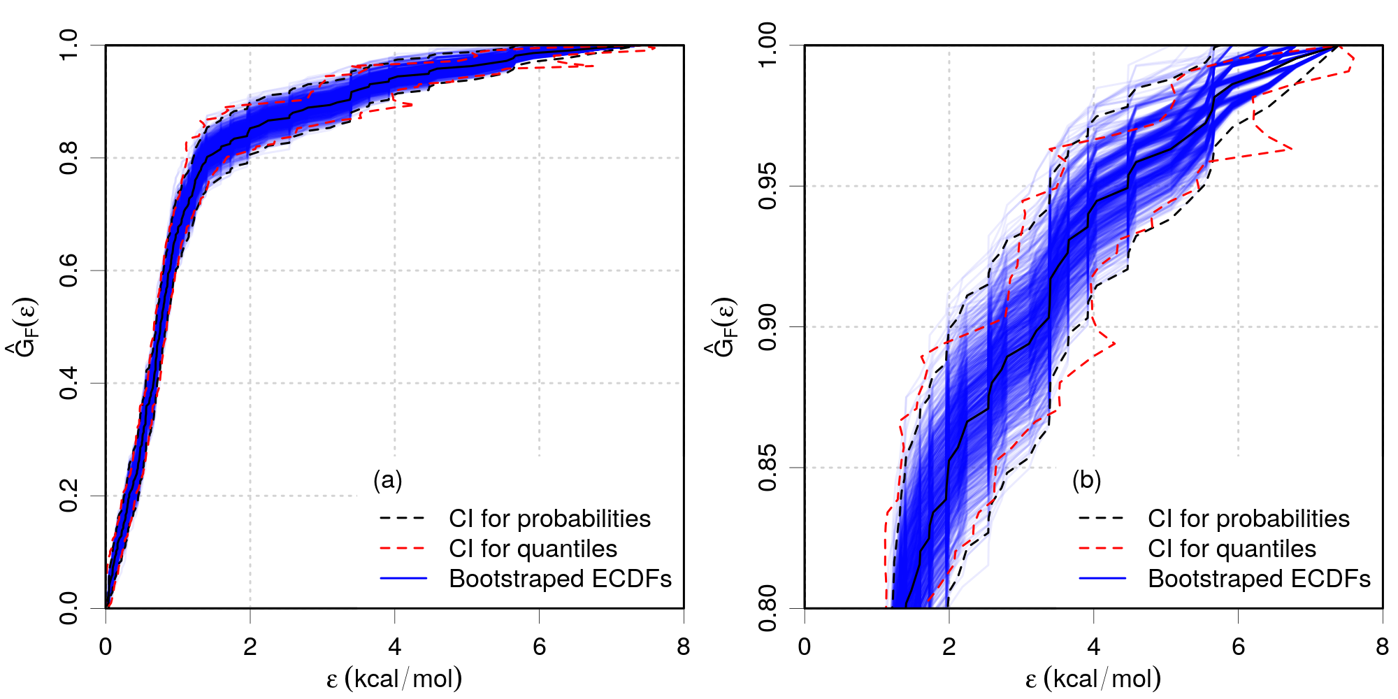
Figure 12: Verification of formulae for vertical and horizontal uncertainties on the ECDF for IAE errors by B3LYP. (a) full probability range; (b) closeup on the high probability range.

Sample size effect.

The results above raise the question of the impact of the sample size on the CI limits of high percentiles. In order to appreciate this effect, we performed a Monte Carlo study by generating 10000 random samples of the folded normal distribution $\pi_{FN}(\epsilon;\mu=0,\sigma=1)$, for sizes between $N=10$ to $500$. For each value of $N$, the mean and 95 % confidence limits of $Q_{90}$ and $Q_{95}$ have been estimated from the sample of 10000 values. The corresponding curves are shown in Fig. 13(a).

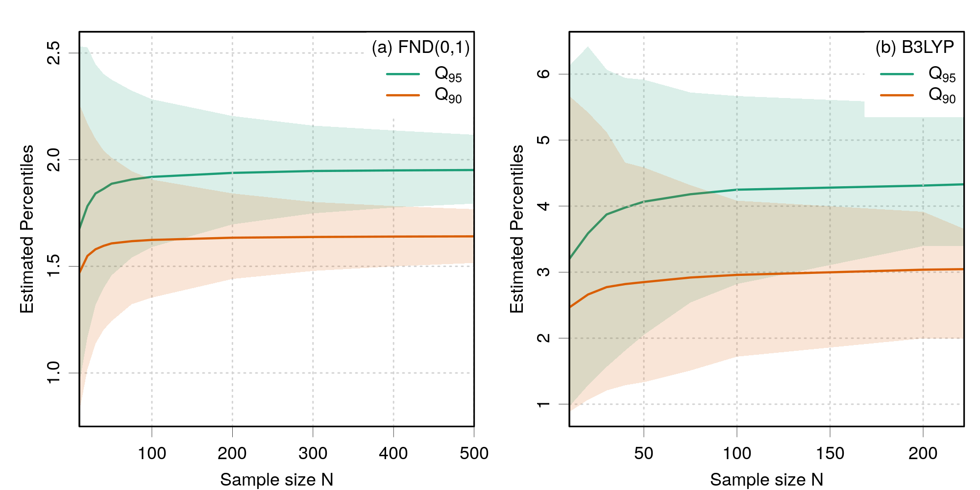
Figure 13: Convergence with the sample size $N$, of the estimated percentiles $Q_{90}$ and $Q_{95}$. (a) folded normal distribution $\pi_{FN}(\epsilon;\mu=0,\sigma=1)$, noted $FND(0,1)$; (b) subsets of the B3LYP error set. Full lines represent the mean value of the percentiles and shaded areas delimit 95 % confidence intervals.

Below $N=100$, there is a strong overlap of the distributions, in the sense that the mean value of one percentile lies within the 95 % CI of the other. Above this value, there is a better discrimination, but one has to wait until $N\simeq 400$ to get non-overlapping 95 % CI intervals.

A similar plot has been done by bootstrapping subsets of the B3LYP data to evaluate the effect of the non-normality of the error distribution on this analysis. One sees in Fig. 13(b) that the conclusions are similar: indiscernibility of $Q_{90}$ and $Q_{95}$ below $N\simeq 100$, with a small overlap of the 95 % CIs around $N=200$.

References

- Pernot et al. (2015) P. Pernot, B. Civalleri, D. Presti, and A. Savin, J. Phys. Chem. A 119, 5288 (2015).
- Proppe and Reiher (2017) J. Proppe and M. Reiher, J. Chem. Theory Comput. 13, 3297 (2017).
- Ruscic (2014) B. Ruscic, Int. J. Quantum Chem. 114, 1097 (2014).
- Irikura, Johnson, and Kacker (2004) K. K. Irikura, R. D. Johnson, and R. N. Kacker, Metrologia 41, 369 (2004).
- Cailliez and Pernot (2011) F. Cailliez and P. Pernot, J. Chem. Phys. 134, 054124 (2011).
- Dunning (2000) T. H. Dunning, J. Phys. Chem. A 104, 9062 (2000).
- Pernot (2017) P. Pernot, J. Chem. Phys. 147, 104102 (2017).
- BIPM et al. (2008) BIPM, IEC, IFCC, ILAC, ISO, IUPAC, IUPAP, and OIML, “Evaluation of measurement data - Guide to the expression of uncertainty in measurement (GUM),” Tech. Rep. 100:2008 (Joint Committee for Guides in Metrology, JCGM, 2008).
- Pople et al. (1989) J. A. Pople, M. Head-Gordon, D. J. Fox, K. Raghavachari, and L. A. Curtiss, J. Chem. Phys. 90, 5622 (1989).
- Raghavachari and Saha (2015) K. Raghavachari and A. Saha, Chem. Rev. 115, 5643 (2015).
- Simm and Reiher (2016) G. N. Simm and M. Reiher, J. Chem. Theory Comput. 12, 2762 (2016).
- Ramakrishnan et al. (2015) R. Ramakrishnan, P. O. Dral, M. Rupp, and O. A. von Lilienfeld, J. Chem. Theory Comput. 11, 2087 (2015).
- Rupp (2015) M. Rupp, Int. J. Quantum Chem. 115, 1058 (2015).
- Wellendorff et al. (2014) J. Wellendorff, K. T. Lundgaard, K. W. Jacobsen, and T. Bligaard, J. Chem. Phys. 140, 144107 (2014).
- Proppe et al. (2016) J. Proppe, T. Husch, G. N. Simm, and M. Reiher, Faraday Discuss. 195, 497 (2016).
- Aldegunde, Kermode, and Zabaras (2016) M. Aldegunde, J. R. Kermode, and N. Zabaras, J. Comput. Phys. 311, 173 (2016).
- Karton, Daon, and Martin (2011) A. Karton, S. Daon, and J. M. L. Martin, Chem. Phys. Lett. 510, 165 (2011).
- (18) L. A. Curtiss, K. Raghavachari, G. W. Trucks, and J. A. Pople, J. Chem. Phys. 94, 7221.
- Peverati and Truhlar (2014) R. Peverati and D. G. Truhlar, Phil. Trans. R. Soc. A 372, 20120476 (2014).
- Wang et al. (2017) Y. Wang, X. Jin, H. S. Yu, D. G. Truhlar, and X. He, Proc. Natl. Acad. Sci. U.S.A. 114, 8487 (2017).
- Note (1) We adopt this acronym in the present study to avoid confusions with atomization energies (AE), used in the application part.
- Civalleri et al. (2012) B. Civalleri, D. Presti, R. Dovesi, and A. Savin, in Chemical Modelling: Applications and Theory, Vol. 9 (Royal Soc. Chem., 2012) pp. 168–185.
- Savin and Johnson (2015) A. Savin and E. R. Johnson, Top. Curr. Chem. 365, 81 (2015).
- Curtiss et al. (2000) L. A. Curtiss, K. Raghavachari, P. C. Redfern, and J. A. Pople, J. Chem. Phys. 112, 7374 (2000).
- Taylor (1997) J. R. Taylor, Introduction To Error Analysis, 2nd ed. (University Science Books, 1997).
- Bevington and Robinson (1992) P. R. Bevington and D. K. Robinson, Data Reduction and Error Analysis for the Physical Sciences (McGraw-Hill, New York, 1992).
- Stuart and Ord (1994) A. Stuart and K. Ord, Kendall’s Advanced Theory of Statistics: Volume 1: Distribution Theory (Wiley, 1994).
- Note (2) These estimators assume that the points in errors samples are not correlated. However, raw error samples often display systematic trends, as observed for some DFAs when sorting the errors by the number of atoms in the molecules (Fig. 6). These patterns corresponding to positive serial correlations, the standard errors are expected to be underestimated.
- Efron (1979) B. Efron, Ann. Stat. 7, 1 (1979).
- Willmott and Matsuura (2005) C. J. Willmott and K. Matsuura, Climate Res. 30, 79 (2005).
- Chai and Draxler (2014) T. Chai and R. R. Draxler, Geosci. Model Dev. 7, 1247 (2014).
- Leone, Nelson, and Nottingham (1961) F. C. Leone, L. S. Nelson, and R. B. Nottingham, Technometrics 3, 543 (1961).
- Klippenstein, Harding, and Ruscic (2017) S. J. Klippenstein, L. B. Harding, and B. Ruscic, J. Phys. Chem. A 121, 6580 (2017).
- Otero-de-la Roza and Johnson (2013) A. Otero-de-la Roza and E. R. Johnson, J. Chem. Phys. 138, 204109 (2013).
- Perdew and Yue (1986) J. P. Perdew and W. Yue, Phys. Rev. B 33, 8800 (1986).
- Perdew, Burke, and Ernzerhof (1996) J. P. Perdew, K. Burke, and M. Ernzerhof, Phys. Rev. Lett. 77, 3865 (1996).
- Lee, Yang, and Parr (1988) C. Lee, W. Yang, and R. G. Parr, Phys. Rev. B 37, 785 (1988).
- Becke (1993) A. D. Becke, J. Chem. Phys. 98, 5648 (1993).
- Adamo and Barone (1999) C. Adamo and V. Barone, J. Chem. Phys. 110, 6158 (1999).
- Yanai, Tew, and Handy (2004) T. Yanai, D. P. Tew, and N. C. Handy, Chem. Phys. Lett. 393, 51 (2004).
- Vydrov and Scuseria (2006) O. A. Vydrov and G. E. Scuseria, J. Chem. Phys. 125, 234109 (2006).
- Vydrov et al. (2006) O. A. Vydrov, J. Heyd, A. V. Krukau, and G. E. Scuseria, J. Chem. Phys. 125, 074106 (2006).
- Becke (1988) A. D. Becke, Phys. Rev. A 38, 3098 (1988).
- Hamprecht et al. (1998) F. A. Hamprecht, A. J. Cohen, D. J. Tozer, and N. C. Handy, J. Chem. Phys. 109, 6264 (1998).
- Perdew et al. (2016) J. P. Perdew, J. Sun, A. J. Garza, and G. E. Scuseria, Z. Phys. Chem. 230, 737 (2016).
- Margraf, Ranasinghe, and Bartlett (2017) J. T. Margraf, D. S. Ranasinghe, and R. J. Bartlett, Phys. Chem. Chem. Phys. 19, 9798 (2017).
- Faver et al. (2011) J. C. Faver, M. L. Benson, X. He, B. P. Roberts, B. Wang, M. S. Marshall, C. D. Sherrill, and K. M. Merz Jr, PLoS ONE 6, e18868 (2011).
- Walters (2013) W. P. Walters, J. Chem. Inf. Model. 53, 1529 (2013).
- Rudshteyn, Acharya, and Batista (2017) B. Rudshteyn, A. Acharya, and V. S. Batista, J. Phys. Chem. C 121, 28212 (2017).
- Note (3) Note that the performances of the studied DFAs for atomization energies could have been significantly improved in two ways: (1) by splitting the G3/99 datasets into CHON and non-CHON subsets; and (2) by correction of the bias and/or trends observed in the error samples Pernot et al. (2015); Ramakrishnan et al. (2015). At the present level of “raw errors”, the percentiles of the unsigned error distributions include prediction bias (). They provide estimates of the expected error amplitude which are therefore pessimistic, in the sense that a simple shift of the results by the MSE would notably improve the situation for many DFAs.
- Medford et al. (2014) A. J. Medford, J. Wellendorff, A. Vojvodic, F. Studt, F. Abild-Pedersen, K. W. Jacobsen, T. Bligaard, and J. K. Norskov, Science 345, 197 (2014).
- Sutton et al. (2016) J. E. Sutton, W. Guo, M. A. Katsoulakis, and D. G. Vlachos, Nat. Chem. 8, 331 (2016).
- Ulissi et al. (2017) Z. W. Ulissi, A. J. Medford, T. Bligaard, and J. K. Nørskov, Nat. Commun. 8, 14621 (2017).
- Pernot and Savin (2017) P. Pernot and A. Savin, Code and data to reproduce the results of the paper "Probabilistic performance estimators for computational chemistry methods: the empirical cumulative distribution function of absolute errors", https://github.com/ppernot/ECDFT (2017).
- R Core Team (2015) R Core Team, R: A Language and Environment for Statistical Computing, R Foundation for Statistical Computing, Vienna, Austria (2015).