Graphical Models for Processing Missing Data

Abstract

This paper reviews recent advances in missing data research using graphical models to represent multivariate dependencies. We first examine the limitations of traditional frameworks from three different perspectives: transparency, estimability and testability. We then show how procedures based on graphical models can overcome these limitations and provide meaningful performance guarantees even when data are Missing Not At Random (MNAR). In particular, we identify conditions that guarantee consistent estimation in broad categories of missing data problems, and derive procedures for implementing this estimation. Finally we derive testable implications for missing data models in both MAR (Missing At Random) and MNAR categories.

Graphical Models for Processing Missing Data

Keywords: Missing data, Graphical Models, Testability, Recoverability, Non-Ignorable, Missing Not At Random (MNAR)

1 Introduction

Missing data present a challenge in many branches of empirical sciences. Sensors do not always work reliably, respondents do not fill out every question in the questionnaire, and medical patients are often unable to recall episodes, treatments or outcomes. The statistical literature on this problem is rich and abundant and has resulted in powerful software packages such as MICE in R, Stata, SAS and SPSS which offer various ways of handling missingness. Most practices are based on the seminal work of Rubin (1976) who formulated procedures and conditions under which the damage due to missingness can be reduced. This theory has also resulted in a number of performance guarantees when data obey certain statistical conditions. However, these conditions are rather strong, and extremely hard to ascertain in real world problems. Little and Rubin (2014)(page 22), summarize the state of the art by observing: “essentially all the literature on multivariate incomplete data assumes that the data are Missing At Random (MAR)”. Indeed, popular estimation methods for missing data such as Maximum Likelihood based techniques (Dempster et al., 1977) and Multiple Imputation (Rubin, 1978) require MAR assumption to guarantee convergence to consistent estimates. Furthermore, it is almost impossible for a practicing statistician to decide whether the MAR condition holds in a given problem. The literature on data that go beyond MAR is quite limited, and lacks systematic methodology for computing consistent estimates when such exist. Some examples include Fitzmaurice et al. (2008), Carpenter and Kenward (2014), Robins (2000) and Scharfstein et al. (1999).

Recent years have witnessed a growing interest in analysing missing data using graphical models to encode assumptions about the reasons for missingness. This development is natural since graphical models provide efficient representation of conditional independencies implied by modeling assumptions. Earlier papers in this development are Daniel et al. (2012) who provided sufficient criteria under which consistent estimates can be computed from complete cases (i.e. samples in which all variables are fully observed).Thoemmes and Rose (2013) (and later on Thoemmes and Mohan (2015)) developed techniques that guide the selection of auxiliary variables to improve estimability from incomplete data. In machine learning, particularly while estimating parameters of Bayesian Networks, graphical models have long been used as a tool when dealing with missing data (Darwiche (2009)).

Table 1: Highlights of Major Results

Criteria and procedures for recovering statistical and causal parameters from missing data
1. We provide methods for recovering conditional distributions in the presence of latent variables.
2. We demonstrate the feasibility of recovering joint distribution in cases where variables cause their own missingness.
3. We identify problems for which recoverability is infeasible.

Tests for challenging compatibility of model with observed data
1. We establish general criteria for testing conditional independence claims.
2. We devise tests for MAR (Missing at Random) models.
3. We identify dependence claims that defy testability.

In this paper we review the contributions of graphical models to missing data research and emphasize three main aspects: (1) Transparency (2) Recoverability (consistent estimation) and (3) Testability. The main results of the paper are highlighted in table 1.

Transparency

Consider a practicing statistician who has acquired a statistical package that handles missing data and would like to know whether the problem at hand meets the requirements of the software. As noted by Little and Rubin (2014) (see appendix 6.1) and many others such as Rhoads (2012) and Balakrishnan (2010), almost all available software packages implicitly assume that data fall under two categories: MCAR (Missing Completely At Random) or MAR (formally defined in section 2.2). Failing this assumption, there is no guarantee that estimates produced by current software will be less biased than those produced by complete case analysis. Consequently, it is essential for the user to decide if the type of missingness present in the data is compatible with the requirements of MCAR or MAR.

Prior to the advent of graphical models, no tool was available to assist in this decision, since the independence conditions that define MCAR or MAR are neither visible in the data, nor in a mathematical model that a researcher can consult to verify those conditions. We will show how graphical models enable an efficient and transparent classification of the missingness mechanism. In particular, the question of whether the data fall into the MCAR or MAR categories can be answered by mere inspection of the graph structure. In addition, we will show how graphs facilitate a more refined, query-specific taxonomy of missingness in MNAR (Missing Not At Random) problems.

The transparency associated with graphical models stems from three factors. First, graphs excel in encoding and detecting conditional independence relations, far exceeding the capacity of human intuition. Second, all assumptions are encoded causally, mirroring the way researchers store qualitative scientific knowledge; direct judgments of conditional independencies are not required, since these can be read off the structure of the graph. Finally, the ultimate aim of all assumptions is to encode “the reasons for missingness” which is a causal, not a statistical concept. Thus, even when our target parameter is purely statistical, say a regression coefficient, causal modeling is still needed for encoding the “process that causes missing data” (Rubin (1976)).

Recoverability (Consistent Estimation)

Recoverability (to be defined formally in Section 3) refers to the task of determining, from an assumed model, whether any method exists that produces a consistent estimate of a desired parameter and, if so, how. If the answer is negative, then an inconsistent estimate should be expected even with large samples, and no algorithm, however smart, can yield a consistent estimate. On the other hand, if the answer is affirmative then there exists a procedure that can exploit the features of the problem to produce consistent estimates. If the problem is MAR or MCAR, standard missing data software can be used to obtain consistent estimates. But if a recoverable problem is MNAR, the user would do well to discard standard software and resort to an estimator based on graphical analysis. In Section 3 of this paper we present several methods of deriving consistent estimators for both statistical and causal parameters.

The general question of recoverability, to the best of our knowledge, has not received due attention in the literature. The notion that some parameters cannot be estimated by any method whatsoever while others can, still resides in an unchartered territory. We will show in Section 3 that most MNAR problems exhibit this dichotomy. That is, problems for which it is impossible to properly impute all missing values in the data, would still permit the consistent estimation of some parameters of interest. More importantly, the estimable parameters can often be identified directly from the structure of the graph.

Testability

Testability asks whether it is possible to tell if any of the model’s assumptions is incompatible with the available data (corrupted by missingness). Such compatibility tests under missingness are hard to come by and the few tests reported in the literature are mostly limited to MCAR (Little, 1988). As stated in Allison (2003), “Worse still, there is no empirical way to discriminate one nonignorable model from another (or from the ignorable model).”. In section 4 we will show that remarkably, discrimination is feasible; MAR problems do have a simple set of testable implications and MNAR problems can often be tested depending on their graph structures.

In summary, although mainstream statistical analysis of missing data problems has made impressive progress in the past few decades, it left key problem areas relatively unexplored, especially those touching on transparency, estimability and testability. This paper casts missing data problems in the language of causal graphs and shows how this representation facilitates solutions to pending problems. In particular, we show how the MCAR, MAR, MNAR taxonomy becomes transparent in the graphical language, how the estimability of a needed parameter can be determined from the graph structure, what estimators would guarantee consistent estimates, and what modeling assumptions lend themselves to empirical scrutiny.

2 Graphical Models for Missing Data: Missingness Graphs (m-graphs)

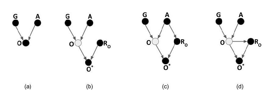
Figure 1: (a)causal graph under no missingness (b), (c) & (d) m-graphs modeling distinct missingness processes.

The following example, inspired by Little and Rubin (2002) (example-1.6, page 8), describes how graphical models can be used to explicitly model the missingness process and encode the underlying causal and statistical assumptions. Consider a study conducted in a school that measured three (discrete) variables: Age (A), Gender (G) and Obesity (O).

No Missingness If all three variables are completely recorded, then there is no missingness. The causal graph depicting the interrelations between variables is shown in Figure 1 (a). Nodes correspond to variables and edges indicate the existence of a causal relationship between pairs of nodes they connect. The value of a child node is a (stochastic) function of the values of its parent nodes. i.e. Obesity is a (stochastic) function of Age and Gender. The absence of an edge between Age and Gender indicates that $A$ and $G$ are independent, denoted by $A\mbox{$\bot\!\!\!\bot$}G$.

Table 2: Missing dataset in which Age and Gender are fully observed and Obesity is partially observed.

$\#$	Age	Gender	Obesity∗	$R_{O}$
1	16	F	Obese	0
2	15	F	$m$	1
3	15	M	$m$	1
4	14	F	Not Obese	0
5	13	M	Not Obese	0
6	15	M	Obese	0
7	14	F	Obese	0

Representing Missingness Assume that Age and Gender are are fully observed since they can be obtained from school records. Obesity however is corrupted by missing values due to some students not revealing their weight. When the value of $O$ is missing we get an empty measurement which we designate by $m$. Table 2 exemplifies a missing dataset. The missingness process can be modelled using a proxy variable Obesity${}^{*}(O^{*})$ whose values are determined by Obesity and its missingness mechanism $R_{O}$.

$$O^{*}=f(R_{O},O)=\left\{\begin{array}[]{l l}O&\quad\text{if }R_{O}=0\\ m&\quad\text{if }R_{O}=1\\ \end{array}\right.$$

$R_{O}$ governs the masking and unmasking of Obesity. When $R_{O}=1$ the value of obesity is concealed i.e. $O^{*}$ assumes the values $m$ as shown in samples 2 and 3 in table 2. When $R_{O}=0$, the true value of obesity is revealed i.e. $O^{*}$ assumes the underlying value of Obesity as shown in samples 1, 4, 5, 6 and 7 in table 2.

Missingness can be caused by random processes or can depend on other variables in the dataset. An example of random missingness is students accidentally losing their questionnaires. This is depicted in figure 1 (b) by the absence of parent nodes for $R_{O}$. Teenagers rebelling and not reporting their weight is an example of missingness caused by a fully observed variable. This is depicted in figure 1 (c) by an edge between $A$ and $R_{O}$. Partially observed variables can be causes of missingness as well. For instance consider obese students who are embarrassed of their obesity and hence reluctant to reveal their weight. This is depicted in figure 1 (d) by an edge between $O$ and $R_{O}$ indicating the $O$ is the cause of its own missingness.

The following subsection formally introduces missingness graphs (m-graphs) as discussed in Mohan et al. (2013).

2.1 Missingness Graphs: Notations and Terminology

Let $G(\mathbf{V},E)$ be the causal DAG where $\mathbf{V}$ is the set of nodes and $E$ is the set of edges. Nodes in the graph correspond to variables in the data set and are partitioned into five categories, i.e.

$\mathbf{V}=V_{o}\cup V_{m}\cup U\cup V^{*}\cup R$

$V_{o}$ is the set of variables that are observed in all records in the population and $V_{m}$ is the set of variables that are missing in at least one record. Variable $X$ is termed as fully observed if $X\in V_{o}$ and partially observed if $X\in V_{m}$. $R_{v_{i}}$ and $V_{i}^{*}$ are two variables associated with every partially observed variable, where $V_{i}^{*}$ is a proxy variable that is actually observed, and $R_{v_{i}}$ represents the status of the causal mechanism responsible for the missingness of $V_{i}^{*}$; formally,

$$v_{i}^{*}=f(r_{v_{i}},v_{i})=\left\{\begin{array}[]{l l}v_{i}&\quad\text{if }r_{v_{i}}=0\\ m&\quad\text{if }r_{v_{i}}=1\\ \end{array}\right.$$ (1)

$V^{*}$ is the set of all proxy variables and $\mathbf{R}$ is the set of all causal mechanisms that are responsible for missingness. $U$ is the set of unobserved nodes, also called latent variables. Unless stated otherwise it is assumed that no variable in $V_{o}\cup V_{m}\cup U$ is a child of an $R$ variable. Two nodes $X$ and $Y$ can be connected by a directed edge i.e. $X\to Y$, indicating that $X$ is a cause of $Y$, or by a bi-directed edge $X<\textendash\textendash>Y$ denoting the existence of a $U$ variable that is a parent of both $X$ and $Y$.

We call this graphical representation a Missingness Graph (or $m$-graph). Figure 1 exemplifies three m-graphs in which $V_{o}=\{A,G\}$, $V_{m}=\{O\}$, $V^{*}=\{O^{*}\}$, $U=\emptyset$ and $R=\{R_{O}\}$. Proxy variables may not always be explicitly shown in m-graphs in order to keep the figures simple and clear. The missing data distribution, $P(V^{*},V_{o},R)$ is referred to as the observed-data distribution and the distribution that we would have obtained had there been no missingness, $P(V_{o},V_{m},R)$ is called as the underlying distribution. Conditional Independencies are read off the graph using the d-separation criterion (Pearl, 2009b). For example, Figure 1 (c) depicts the independence $R_{O}\mbox{$\bot\!\!\!\bot$}O|A$ but not $R_{O}\mbox{$\bot\!\!\!\bot$}G|O$.

2.2 Classification of Missing Data Problems based on Missingness Mechanism

Rubin (1976) classified missing data into three categories: Missing Completely At Random (MCAR), Missing At Random (MAR) and Missing Not At Random (MNAR) based on the statistical dependencies between the missingness mechanisms ($R$ variables) and the variables in the dataset $(V_{m},V_{o})$. We capture the essence of this categorization in graphical terms below.

1. Data are MCAR if $V_{m}\cup V_{o}\cup U\mbox{$\bot\!\!\!\bot$}R$ holds in the m-graph. In words, missingness occurs completely at random and is entirely independent of both the observed and the partially observed variables. This condition can be easily identified in an m-graph by the absence of edges between the $R$ variables and variables in $V_{o}\cup V_{m}$.

2. Data are MAR if $V_{m}\cup U\mbox{$\bot\!\!\!\bot$}R|V_{o}$ holds in the m-graph. In words, conditional on the fully observed variables $V_{o}$, missingness occurs at random. In graphical terms, MAR holds if (i) no edges exist between an $R$ variable and any partially observed variable and (ii) no bidirected edge exists between an $R$ variable and a fully observed variable. MCAR implies MAR, ergo all estimation techniques applicable to MAR can be safely applied to MCAR.

3. Data that are not MAR or MCAR fall under the MNAR category.

m-graphs in figure 1 (b), (c) and (d) are typical examples of MCAR, MAR and MNAR categories, respectively. Notice the ease with which the three categories can be identified. Once the user lays out the interrelationships between the variables in the problem, the classification is purely mechanical.

2.2.1 Missing At Random: A Brief Discussion

The original classification used in Rubin (1976) is very similar to the one defined in the preceding paragraphs. The main distinction rests on the fact that MAR defined in Rubin (1976) (which we call Rubin-MAR) is defined in terms of conditional independencies between events where as that in this paper (referred to as MAR) is defined in terms of conditional independencies between variables. Clearly, we can have the former without the latter, in practice though it is rare that scientific knowledge can be articulated in terms of event based independencies that are not implied by variable based independencies.

Over the years the classification proposed in Rubin (1976) has been criticized both for its nomenclature and its opacity. Several authors noted that MAR is a misnomer (Scheffer (2002); Peters and Enders (2002); Meyers et al. (2006); Graham (2009)) noting that randomness in this class is critically conditioned on observed data.

However, the opacity of the assumptions underlying Rubin’s MAR presents a more serious problem. Clearly, a researcher would find it cognitively taxing, if not impossible to even decide if any of these independence assumptions is reasonable. This, together with the fact that Rubin-MAR is untestable (Allison (2002)) motivates the variable-based taxonomy presented above. Seaman et al. (2013) and Doretti et al. (2018) provide another taxonomy and a different perspective on Rubin-MAR.

Nonetheless, Rubin-MAR has an interesting theoretical property: It is the weakest simple condition under which the process that causes missingness can be ignored while still making correct inferences about the data (Rubin, 1976). It was probably this theoretical result that changed missing data practices in the 1970’s. The popular practice prior to 1976 was to assume that missingness was caused totally at random (Gleason and Staelin (1975); Haitovsky (1968)). With Rubin’s identification of the MAR condition as sufficient for drawing correct inferences, MAR became the main focus of attention in the statistical literature.

Estimation procedures such as Multiple Imputation were developed and implemented with MAR assumptions in mind, and popular textbooks were authored exclusively on MAR and its simplified versions (Graham, 2012). In the absence of recognizable criterion for MAR, some authors have devised heuristics invoking auxiliary variables, to increase the chance of achieveing MAR (Collins et al., 2001). Others have warned against indiscriminate inclusion of such variables (Thoemmes and Rose, 2013; Thoemmes and Mohan, 2015). These difficulties have engendered a culture with a tendency to blindly assume MAR, with the consequence that the more commonly occurring MNAR class of problems remains relatively unexplored (Resseguier et al., 2011; Adams, 2007; Osborne, 2012, 2014; Sverdlov, 2015; van Stein and Kowalczyk, 2016).

In his seminal paper (Rubin, 1976) Rubin recommended that researchers explicitly model the missingness process:

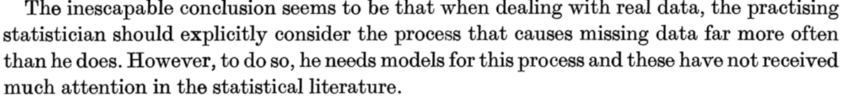
Figure 2: Quote from Rubin (1976)

This recommendation invites in fact the graphical tools described in this paper, for they encourage investigators to model the details of the missingness process rather than blindly assume MAR. These tools have further enabled researchers to extend the analysis of estimation to the vast class of MNAR problems.

In the next section we discuss how graphical models accomplish these tasks.

3 Recoverability

Recoverability addresses the basic question of whether a quantity/parameter of interest can be estimated from incomplete data as if no missingness took place, that is, the desired quantity can be estimated consistently from the available (incomplete) data. This amounts to expressing the target quantity $Q$ in terms of the observed-data distribution $P(V^{*},V_{O},R)$. Typical target quantities that shall be considered are conditional/joint distributions and conditional causal effects.

Definition 1 (Recoverability of target quantity $Q$)

Let $A$ denote the set of assumptions about the data generation process and let $Q$ be any functional of the underlying distribution $P(V_{m},V_{O},R)$. $Q$ is recoverable if there exists a procedure that computes a consistent estimate of $Q$ for all strictly positive observed-data distributions $P(V^{*},V_{o},R)$ that may be generated under $A$.

Since we encode all assumptions in the structure of the m-graph $G$, recoverability becomes a property of the pair {$Q,G$}, and not of the data. We restrict the definition above to strictly positive observed-data distributions, $P(V^{*},V_{o},R)$ except for instances of zero probabilities as specified in equation 1. The reason for this restriction can be understood as the need for observing some unmasked cases for all combinations of variables, otherwise, masked cases can be arbitrary. We note however that recoverability is sometimes feasible even when strict positivity does not hold (Mohan et al. (2013), definition 5 in appendix).

We now demonstrate how a joint distribution is recovered given MAR data.

Example 1

Consider the problem of recovering the joint distribution given the $m$-graph in Fig. 1 (c) and dataset in table 3. Let it be the case that 15-18 year olds were reluctant to reveal their weight, thereby making $O$ a partially observed variable i.e. $V_{m}=\{O\}$ and $V_{o}=\{G,A\}$. This is a typical case of MAR missingness, since the cause of missingness is the fully observed variable: Age. The following three steps detail the recovery procedure.

1. Factorization: The joint distribution may be factorized as:

$$P(G,O,A) =P(G,O|A)P(A)$$

2. Transformation into observables: $$G (G,O)\mbox{$\bot\!\!\!\bot$}R_{O}|A A (G,O) R_{O}$$ implies the conditional independence since d-separates from . Thus,

$$P(G,O,A) =P(G,O|A,R_{O}=0)P(A)$$

3. Conversion of partially observed variables into proxy variables: $$R_{O}=0 O^{*}=O$$ implies (by eq 1). Therefore,

$$P(G,O,A) =P(G,O^{*}|A,R_{O}=0)P(A)$$ (2)

The RHS of Eq. (2) is expressed in terms of variables in the observed-data distribution. Therefore, $P(G,A,O)$ can be consistently estimated (i.e. recovered) from the available data. The recovered joint distribution is shown in table 4.

Table 3: observed-data Distribution $P(G,A,O^{*},R_{O})$ where Gender $(G)$ and Age $(A)$ are fully observed, Obesity $O$ is corrupted by missing values and Obesity’s proxy $(O^{*})$ is observed in its place. Age is partitioned into three groups: $[10-13),[13-15),[15-18)$. Gender and Obesity are binary variables and can take values Male (M) and Female (F), and Yes (Y) and No (N), respectively. The probabilities $p_{1},p_{2},..p_{18}$ stand for the (asymptotic) frequencies of the samples falling in the 18 cells ($G,A,O^{*},R_{O}$).

$G$	$A$	$O^{*}$	$R_{O}$	$P(G,A,O^{*},R_{O})$
M	$10-13$	Y	$0$	$p_{1}$
M	$13-15$	Y	$0$	$p_{2}$
M	$15-18$	Y	$0$	$p_{3}$
M	$10-13$	N	$0$	$p_{4}$
M	$13-15$	N	$0$	$p_{5}$
M	$15-18$	N	$0$	$p_{6}$
F	$10-13$	Y	$0$	$p_{7}$
F	$13-15$	Y	$0$	$p_{8}$
F	$15-18$	Y	$0$	$p_{9}$

$G$	$A$	$O^{*}$	$R_{O}$	$P(G,A,O^{*},R_{O})$
F	$10-13$	N	$0$	$p_{10}$
F	$13-15$	N	$0$	$p_{11}$
F	$15-18$	N	$0$	$p_{12}$
M	$10-13$	$m$	$1$	$p_{13}$
M	$13-15$	$m$	$1$	$p_{14}$
M	$15-18$	$m$	$1$	$p_{15}$
F	$10-13$	$m$	$1$	$p_{16}$
F	$13-15$	$m$	$1$	$p_{17}$
F	$15-18$	$m$	$1$	$p_{18}$

Table 4: Recovered joint distribution corresponding to dataset in table 3 and m-graph in figure 1(c)

$G$	$A$	$O$	$P(G,O,A)$
M	$10-13$	Y	$\frac{p_{1}*(p_{1}+p_{4}+p_{7}+p_{10}+p_{13}+p_{16})}{p_{1}+p_{4}+p_{7}+p_{10}}$
M	$13-15$	Y	$\frac{p_{2}*(p_{2}+p_{5}+p_{8}+p_{11}+p_{14}+p_{17})}{p_{2}+p_{5}+p_{8}+p_{11}}$
M	$15-18$	Y	$\frac{p_{3}*(p_{3}+p_{6}+p_{9}+p_{12}+p_{15}+p_{18})}{p_{3}+p_{6}+p_{9}+p_{12}}$
M	$10-13$	N	$\frac{p_{4}*(p_{1}+p_{4}+p_{7}+p_{10}+p_{13}+p_{16})}{p_{1}+p_{4}+p_{7}+p_{10}}$
M	$13-15$	N	$\frac{p_{5}*(p_{2}+p_{5}+p_{8}+p_{11}+p_{14}+p_{17})}{p_{2}+p_{5}+p_{8}+p_{11}}$
M	$15-18$	N	$\frac{p_{6}*(p_{3}+p_{6}+p_{9}+p_{12}+p_{15}+p_{18})}{p_{3}+p_{6}+p_{9}+p_{12}}$

$G$	$A$	$O$	$P(G,O,A)$
F	$10-13$	Y	$\frac{p_{7}*(p_{1}+p_{4}+p_{7}+p_{10}+p_{13}+p_{16})}{p_{1}+p_{4}+p_{7}+p_{10}}$
F	$13-15$	Y	$\frac{p_{8}*(p_{2}+p_{5}+p_{8}+p_{11}+p_{14}+p_{17})}{p_{2}+p_{5}+p_{8}+p_{11}}$
F	$15-18$	Y	$\frac{p_{9}*(p_{3}+p_{6}+p_{9}+p_{12}+p_{15}+p_{18})}{p_{3}+p_{6}+p_{9}+p_{12}}$
F	$10-13$	N	$\frac{p_{10}*(p_{1}+p_{4}+p_{7}+p_{10}+p_{13}+p_{16})}{p_{1}+p_{4}+p_{7}+p_{10}}$
F	$13-15$	N	$\frac{p_{11}*(p_{2}+p_{5}+p_{8}+p_{11}+p_{14}+p_{17})}{p_{2}+p_{5}+p_{8}+p_{11}}$
F	$15-18$	N	$\frac{p_{12}*(p_{3}+p_{6}+p_{9}+p_{12}+p_{15}+p_{18})}{p_{3}+p_{6}+p_{9}+p_{12}}$

Note that samples in which obesity is missing are not discarded but are used instead to update the weights $p_{1},..p_{12}$ of the cells in which obesity is has a definite value. This can be seen by the presence of probabilities $p_{13},...p_{18}$ in table 4 and the fact that samples with missing values have been utilized to estimate prior probability $P(A)$ in equation 2. Note also that the joint distribution permits an alternative decomposition:

$$P(G,O,A) =P(O|A,G)P(A,G)$$

$$=P(O^{*}|A,G,R_{O}=0)P(A,G)$$

The equation above licenses a different estimation procedure whereby $P(A,G)$ is estimated from all samples, including those in which obesity is missing, and only the estimation of $P(O^{*}|A,G,R_{O}=0)$ is restricted to the complete samples. The efficiency of various decompositions are analysed in Van den Broeck et al. (2015); Mohan et al. (2014).

Finally we observe that for the MCAR m-graph in figure 1 (b), a wider spectrum of decompositions is applicable, including:

$$P(G,O,A) =P(O,A,G|R_{O}=0)$$

$$=P(O^{*},A,G|R_{O}=0)$$

The equation above licenses the estimation of the joint distribution using only those samples in which obesity is observed. This estimation procedure, called listwise deletion or complete-case analysis (Little and Rubin, 2002), would usually result in wastage of data and lower quality of estimate, especially when the number of samples corrupted by missingness is high. Considerations of estimation efficiency should therefore be applied once we explicate the spectrum of options licensed by the m-graph.

A completely different behavior will be encountered in the model of 1 (d) which, as we have noted, belong to the MNAR category. Here, the arrow $O\to R_{O}$ would prevent us from executing step 2 of the estimation procedure, that is, transforming $P(G,O,A)$ into an expression involving solely observed variables. We can in fact show that in this example the joint distribution is nonrecoverable. That is, regardless of how large the sample or how clever the imputation, no algorithm exists that produces consistent estimate of P(G,O,A).

The possibility of encountering non-recoverability is not discussed as often as it ought to be in mainstream missing data literature mostly because the MAR assumption is either taken for granted (Pfeffermann and Sikov, 2011) or thought of as a good approximation for MNAR (Chang, 2011). Consequently it is often presumed that the maximum likelihood method can deliver a consistent estimate of any desired parameter. While it is true for MAR, it is certainly not true in cases for which we can prove non-recoverability, and requires model-based analysis for MNAR.

Remark 1

Observe that equation 2 yields an estimand for the query, $P(G,O,A)$, as opposed to an estimator. An estimand is a functional of the observed-data distribution, $P(V^{*},R,V_{o})$, whereas an estimator is a rule detailing how to calculate the estimate from measurements in the sample. Our estimands naturally give rise to a closed form estimator, for instance, the estimator corresponding to the estimand in equation 2 is:
$\frac{\#(G=g,O^{*}=o,A=a,R_{O}=0)}{\#(A=a,R_{O}=0)}\frac{\#(A=a)}{N}$, where $N$ is the total number of samples collected and $\#(X_{1}=x_{1},X_{2}=x_{2},...X_{j}=x_{j})$ is the frequency of the event $x_{1},x_{2},...x_{j}$. Algorithms inspired by such closed form estimation techniques were shown in Van den Broeck et al. (2015), to outperform conventional methods such as EM computationally, for instance by scaling to networks where it is intractable to run even one iteration of EM. Such algorithms are indispensable for large scale and big data learning tasks in machine learning and artificial intelligence for which EM is not a viable option.

Recovering from Complete & Available cases

Traditionally there has been great interest in complete case analysis primarily due to its simplicity and ease of applicability. However, it results in a large wastage of data and a more economical version of it, called available case analysis would generally be more desirable. The former retains only samples in which variables in the entire dataset are observed, whereas the latter retains all samples in which the variables in the query are observed. Sufficient criterion for recovering conditional distributions from complete cases as well as available cases is widely discussed in literature( Bartlett et al. (2014); Little and Rubin (2002); White and Carlin (2010)) and we state them in the form of a corollary below:

Corollary 1

(a) Given m-graph $G$, $P(X|Y)$ is recoverable from complete cases if $X\mbox{$\bot\!\!\!\bot$}R|Y$ holds in $G$ where $R$ is the set of all missingness mechanisms.
(b) Given m-graph $G$, $P(X|Y)$ is recoverable from available cases if $X\mbox{$\bot\!\!\!\bot$}(Rx,Ry)|Y$ holds in $G$.

In figure 3 for example, we see that $Z_{1}\mbox{$\bot\!\!\!\bot$}R_{Z_{1}}$ holds but $Z\mbox{$\bot\!\!\!\bot$}R_{x}$ does not. Therefore $P(Z_{1})$ is recoverable from available cases but not complete cases.

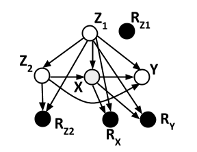
Figure 3: m-graphs depicting MNAR in which $P(Y|X,Z_{1},Z_{2})$ is recoverable. Proxy variables have not been explicitly portrayed as stated in section 2.1.

A generic example for recoverability under MNAR is presented below.

Example 2 (Recoverability in MNAR m-graphs)

Consider the m-graph $G$ in figure 3 where all variables are subject to missingness. $Y$ is the outcome of interest, $X$ the exposure of interest and $Z_{1}$ and $Z_{2}$ are baseline covariates. The target parameter is $P(Y|X,Z_{1},Z_{2})$, the regression of $Y$ on $X$ given both baseline covariates.
Since $Y\mbox{$\bot\!\!\!\bot$}(R_{X},R_{Y},R_{Z_{1}},R_{Z_{2}})|(X,Z_{1},Z_{2})$ in $G$, $P(Y|X,Z_{1},Z_{2})$ can be recovered as:

$$P(Y|X,Z_{1},Z_{2}) =P(Y|(X,Z_{1},Z_{2},R_{X}=0,R_{Y}=0,R_{Z_{1}}=0,R_{Z_{2}}=0))$$

$$=P(Y^{*}|(X^{*},Z_{1}^{*},Z_{2}^{*},R_{X}=0,R_{Y}=0,R_{Z_{1}}=0,R_{Z_{2}}=0))\mbox{( Using eq \ref{eq:miss1})}$$

Note that despite the fact that all variables are subject to missingness and missingness is highly dependent on partially observed variables the graph nevertheless licenses the estimation of the target parameter from samples in which all variables are observed.

In the following subsection we define the notion of Ordered factorization which leads to a criterion for sequentially recovering conditional probability distributions (Mohan et al. (2013); Mohan and Pearl (2014a)).

3.1 Recovery by Sequential Factorization

Definition 2 (Ordered factorization of $P(Y|Z)$)

Let $Y_{1}<Y_{2}<\ldots<Y_{k}$ be an ordered set of all variables in $Y$, $1\leq i\leq|Y|=k$ and $X_{i}\subseteq\{Y_{i+1},\ldots,Y_{n}\}\cup Z$. Ordered factorization of $P(Y|Z)$ is the product of conditional probabilities i.e. $P(Y|Z)=\prod_{i}P(Y_{i}|X_{i})$, such that $X_{i}$ is a minimal set for which $Y_{i}\mbox{$\bot\!\!\!\bot$}(\{Y_{i+1},\ldots,Y_{n}\}\setminus X_{i})|X_{i}$ holds.

The following theorem presents a sufficient condition for recovering conditional distributions of the form $P(Y|X)$ where $\{Y,X\}\subseteq V_{m}\cup V_{o}$.

Theorem 1

Given an m-graph $G$ and a observed-data distribution $P(V^{*},V_{o},R)$, a target quantity $Q$ is recoverable if $Q$ can be decomposed into an ordered factorization, or a sum of such factorizations, such that every factor $Q_{i}=P(Y_{i}|X_{i})$ satisfies $Y_{i}\mbox{$\bot\!\!\!\bot$}(R_{y_{i}},R_{x_{i}})|X_{i}$. Then, each $Q_{i}$ may be recovered as $P(Y^{*}_{i}|X^{*}_{i},R_{Y_{i}}=0,R_{X_{i}}=0)$.

An ordered factorization that satisfies theorem 1 is called as an admissible factorization.

Example 3

Consider the problem of recovering $P(X,Y)$ given $G$, the m-graph in figure 4 (a). $G$ depicts an MNAR problem since missingness in $Y$ is caused by the partially observed variable $X$. The factorization $P(Y|X)P(X)$ is admissible since both $Y\mbox{$\bot\!\!\!\bot$}R_{x},R_{y}|X$ and $X\mbox{$\bot\!\!\!\bot$}R_{x}$ hold in $G$. $P(X,Y)$ can thus be recovered using theorem 1 as $P(Y^{*}|X^{*},R_{x}=0,R_{y}=0)P(X^{*}|R_{x}=0)$. Here, complete cases are used to estimate $P(Y|X)$ and all samples including those in which Y is missing are used to estimate $P(X)$. Note that the decomposition $P(X|Y)P(Y)$ is not admissible.

Corollary 2

Given an m-graph $G$ depicting MAR joint distribution is recoverable in $G$ as $P(V_{o},V_{m})=P(V^{*}|V_{o},R=0)P(V_{o})$.

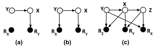
Figure 4: m-graphs from which joint and/or conditional distributions can be recovered using various factorizations.

3.2 R Factorization

Example 4

Consider the problem of recovering $Q=P(X,Y)$ from the $m$-graph of Figure 4(b). Interestingly, no ordered factorization over variables $X$ and $Y$ would satisfy the conditions of Theorem 1. To witness we write $P(X,Y)=P(Y|X)P(X)$ and note that the graph does not permit us to augment any of the two terms with the necessary $R_{x}$ or $R_{y}$ terms; $X$ is independent of $R_{x}$ only if we condition on $Y$, which is partially observed, and $Y$ is independent of $R_{y}$ only if we condition on $X$ which is also partially observed. This deadlock can be disentangled however using a non-conventional decomposition:

$$Q =P(X,Y)=P(X,Y)\frac{P(R_{x}=0,R_{y}=0|X,Y)}{P(R_{x}=0,R_{y}=0|X,Y)}$$

$$=\frac{P(R_{x}=0,R_{y}=0)P(X,Y|R_{x}=0,R_{y}=0)}{P(R_{x}=0|Y,R_{y}=0)P(R_{y}=0|X,R_{x}=0)}$$

where the denominator was obtained using the independencies $R_{x}\mbox{$\bot\!\!\!\bot$}(X,R_{y})|Y$ and
$R_{y}\mbox{$\bot\!\!\!\bot$}(Y,R_{x})|X$ shown in the graph. The final expression below,

$$P(X,Y) =\frac{P(R_{x}=0,R_{y}=0)P(X^{*},Y^{*}|R_{x}=0,R_{y}=0)}{P(R_{x}=0|Y^{*},R_{y}=0)P(R_{y}=0|X^{*},R_{x}=0)}\mbox{ (Using equation \ref{eq:miss1})}$$ (3)

which is in terms of variables in the observed-data distribution, renders $P(X,Y)$ recoverable. This example again shows that recovery is feasible even when data are MNAR.

The following theorem (Mohan et al. (2013); Mohan and Pearl (2014a)) formalizes the recoverability scheme exemplified above.

Theorem 2 (Recoverability of the Joint $P(V)$)

Given a $m$-graph $G$ with no edges between $R$ variables the necessary and sufficient condition for recovering the joint distribution $P(V)$ is the absence of any variable $X\in V_{m}$ such that:
1. $X$ and $R_{x}$ are neighbors
2. $X$ and $R_{x}$ are connected by a path in which all intermediate nodes are colliders and elements of $V_{m}\cup V_{o}$. When recoverable, $P(V)$ is given by

$$P(v)=\frac{P(R=0,v)}{\prod_{i}P(R_{i}=0|Mb^{o}_{r_{i}},Mb^{m}_{r_{i}},R_{Mb^{m}_{r_{i}}}=0)},$$ (4)

where $Mb^{o}_{r_{i}}\subseteq V_{o}$ and $Mb^{m}_{r_{i}}\subseteq V_{m}$ are the markov blanket of $R_{i}$.

The preceding theorem can be applied to immediately yield an estimand for joint distribution. For instance, given the m-graphs in figure 4 (c), joint distribution can be recovered in one step yielding:

$P(X,Y,Z)=\frac{P(X,Y,Z,R_{x}=0,R_{y}=0,R_{z}=0)}{P(R_{x}=0|Y,R_{y}=0,Z,R_{z}=0)P(R_{y}=0|X,R_{x}=0,Z,R_{z}=0)P(R_{z}=0|Y,R_{y}=0,X,R_{x}=0)}$

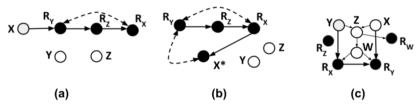
Figure 5: (a) & (c) m-graphs from which conditional distributions can be recovered aided by intervention, (b) latent structure (Pearl (2009b), chapter 2) corresponding to m-graph in (a) when $X$ is treated as a latent variable.

3.3 Constraint Based Recoverability

The recoverability procedures presented thus far relied entirely on conditional independencies that are read off the m-graph using d-separation criterion. Interestingly, recoverability can sometimes be accomplished by graphical patterns other than conditional independencies. These patterns represent distributional constraints which can be detected using mutilated versions of the m-graph. We describe below an example of constraint based recovery.

Example 5

Let $G$ be the m-graph in figure 5 (a) and let the query of interest be $P(X)$. The absence of a set that d-separates $X$ from $R_{x}$, makes it impossible to apply any of the techniques discussed previously. While it may be tempting to conclude that $P(X)$ is not recoverable, we prove otherwise by using the fact that $X\mbox{$\bot\!\!\!\bot$}R_{x}$ holds in the ratio distribution $\frac{P(X,R_{y},R_{z},R_{x})}{P(R_{z}|R_{y})}$. Such ratios are called interventional distributions and the resulting constraints are called Verma Constraints (Verma and Pearl (1991); Tian and Pearl (2002)). The proof presented below employs the rules of do-calculus, to extract these constraints.

$$P(X) =P(X|do(R_{z}=0))\mbox{ (Rule-3 of do-calculus)}$$

$$=P(X|do(R_{z}=0),R_{x}=0)\mbox{ (Rule-1 of do-calculus)}$$

$$=P(X^{*}|do(R_{z}=0),R_{x}=0)\mbox{ (using equation \ref{eq:miss1})}$$

$$=\sum_{R_{Y}}P(X^{*},R_{Y}|do(R_{z}=0),R_{x}=0)$$ (5)

Note that the query of interest is now a function of $$X^{*} X$$ and not . Therefore the problem now amounts to identifying a conditional interventional distribution using the m-graph in figure 5(b). A complete analysis of such problems is available in Shpitser and Pearl (2006) which identifies the causal effect in eq 5 as:

$$P(X) =\sum_{R_{Y}}P(X^{*}|R_{Y},R_{x}=0,R_{z}=0)\frac{P(R_{x}=0|R_{y},R_{z}=0)P(R_{y})}{\sum_{R_{Y}}P(R_{x}=0|R_{y},R_{z}=0)P(R_{y})}$$ (6)

In addition to $P(X)$, this graph also allows recovery of joint distribution as shown below. $P(X,Y,Z)=P(X)P(Y)P(Z)$
$P(X,Y,Z)=\big{(}\sum_{R_{Y}}P(X^{*}|R_{Y},R_{x}=0,R_{z}=0)\frac{P(R_{x}=0|R_{y},R_{z}=0)P(R_{y})}{\sum_{R_{Y}}P(R_{x}=0|R_{y},R_{z}=0)P(R_{y})}\big{)}\\ \hskip 284.52756ptP(Y^{*}=Y|R_{y}=0)P(Z^{*}|R_{z}=0)$

The decomposition in the first line uses $(X,Y)\mbox{$\bot\!\!\!\bot$}Z$ and $X\mbox{$\bot\!\!\!\bot$}Y$. Recoverability of $P(X)$ in the second line follows from equation 6. Theorem 1 can be applied to recover, $P(Y)$ and $P(Z)$, since $Y\mbox{$\bot\!\!\!\bot$}R_{Y}$ and $Z\mbox{$\bot\!\!\!\bot$}R_{Z}$.

Remark 2

In the preceding example we were able to recover a joint distribution despite the fact that the distribution $P(X,R_{Y},R_{x})$ is void of independencies. The ability to exploit such cases further underscores the need for graph based analysis.

The field of epidemiology has several impressive works dealing with coarsened data (Gill et al. (1997); Gill and Robins (1997)) and missing data (Robins (2000, 1997); Robins et al. (2000); Li et al. (2013)). Many among these are along the lines of estimation (mainly of causal queries); Robins et al. (1994) and Rotnitzky et al. (1998) deal with Inverse Probability Weighting based estimators, and Bang and Robins (2005) demonstrates the efficacy of Doubly Robust estimators using simulation studies. The recovery strategy of these existing works are different from that discussed in this paper with the main difference being that these works proceed by intervening on the $R$ variable and thus converting the missing data problem into that of identification of causal effect. For example the problem of recovering $P(X)$ is transformed into that of identifying the counterfactual query $P(X^{*}_{R_{x}=0})$ (which in our framework translates to identifying $P(X^{*}|do(R_{x}=0))$) in the graph in which $X$ is treated as a latent variable. This technique while applicable in several cases is not general and may not always be relied upon to establish recoverability. An example is the problem of recovering joint distribution $P(W,X,Y,Z)$ in figure 5 (c). In this case the equivalent causal query $P(W^{*},X^{*},Y^{*},Z^{*}|do(R_{x}=0,R_{y}=0,R_{w}=0,R_{z}=0))$ is not identifiable in the graph in which $W,X,Y$ and $Z$ are treated as latent variables. The procedure for recovering joint distribution from the m-graph in figure 5 (c) is presented in Appendix 6.2.

3.4 Overcoming Impediments to Recoverability

This section focuses on MNAR problems that are not recoverable. One such problem is elucidated in the following example.

Example 6

Consider a missing dataset comprising of a single variable, Income ($I$), obtained from a population in which the very rich and the very poor were reluctant to reveal their income. The underlying process can be described as a variable causing its own missingness. The m-graph depicting this process is $I\to R_{I}$. Obviously, under these circumstances the true distribution over income, $P(I)$, cannot be computed error-free even if we were given infinitely many samples.

The following theorem identifies graphical conditions that forbid recoverability of conditional probability distributions (Mohan and Pearl (2014a)).

Theorem 3

Let $X\cup Y\subseteq V_{m}\cup V_{o}$ and $|X|=1$. $P(X|Y)$ is not recoverable if either, $X$ and $R_{X}$ are neighbors or there exists a path from $X$ to $R_{x}$ such that all intermediate nodes are colliders and elements of $Y$.

Quite surprisingly, it is sometimes possible to recover joint distributions given m-graphs with graphical structures stated in theorem 3 by jointly harnessing features of the data and m-graph. We exemplify such recovery with an example.

Example 7

Consider the problem of recovering $P(Y,I)$ given the m-graph $G:$ $Y\to I\to R_{I}$, where $Y$ is a binary variable that denotes whether candidate has sufficient years of relevant work experience and $I$ indicates income. $I$ is also a binary variable and takes values high and low. $P(Y)$ is implicitly recoverable since $Y$ is fully observed. $P(Y|I)$ may be recovered as shown below:

$$P(Y|I) =P(Y|I,r^{\prime}_{I})\mbox{ (using $Y\mbox{$\bot\!\!\!\bot$}R_{I}|I$)}$$

$$=P(Y^{*}=Y|I^{*}=I,,r^{\prime}_{I})\mbox{ (using equation \ref{eq:miss1}) }$$

Expressing $P(Y)=\sum_{y}P(Y|I)P(I)$ in matrix form, we get:

$$\left(\begin{array}[]{c}P(y^{\prime})\\ P(y)\end{array}\right)=\left(\begin{array}[]{cc}P(y^{\prime}|i^{\prime})&P(y^{\prime}|i)\\ P(y|i^{\prime})&P(y|i)\end{array}\right)\left(\begin{array}[]{c}P(i^{\prime})\\ P(i)\end{array}\right)$$

Assuming that the square matrix on R.H.S is invertible, $P(I)$ can be estimated as:

$$\left(\begin{array}[]{cc}P(y^{\prime}|i^{\prime})&P(y^{\prime}|i)\\ P(y|i^{\prime})&P(y|i)\end{array}\right)^{-1}\left(\begin{array}[]{c}P(y^{\prime})\\ P(y)\end{array}\right)$$

Having recovered $P(I)$, the query $P(I,Y)$ may be recovered as $P(Y|I)P(I)$.

General procedures for handling non-recoverable cases using both data and graph is discussed in Mohan (2018). The preceding recoverability procedure was inspired by similar results in causal inference (Pearl, 2009a; Kuroki and Pearl, 2014). In contrast to Pearl (2009a) that relied on external studies to compute causal effect in the presence of an unmeasured confounder, Kuroki and Pearl (2014) showed how the same could be effected without external studies. In missing data settings we have access to partial information that allows us to compute conditional distributions. This allows us to adapt the procedure in Pearl (2009a) to establish recoverability. Yet another way of handling these problems is based on double sampling wherein after the initial data collection a a random sample of non-respondents are tracked and their outcomes ascertained (Holmes et al., 2018; Zhang et al., 2016).

3.5 Recovering Causal Effects

We assume the reader is familiar with the basic notions of ”causal queries”, ”causal effect” and ”identifiability” as described in Pearl (2009b) (chapter 3) and Pearl (2009a). Given a causal query and a causal graph with no missingness, we can always determine whether or not the query is identifiable using the complete algorithm in Shpitser and Pearl (2006) or Huang and Valtorta (2006) which outputs an estimand whenever identifiability holds. In the presence of missingness, a necessary condition for recoverability of a causal query is its identifiability in the substantive model i.e. the subgraph comprising of $V_{o},$ $V_{m}$ and $U$. In other words, a query which is not identifiable in this model will not be recoverable under missingness. A canonical example of such case is the bow-arc graph (figure 7 (c)) for which the query $P(Y|do(X=x))$ is known to be non-identifiable (Pearl (2009b)) In the remainder of this subsection we will assume that queries of interest are identifiable in the substantive model, and our task is to determine whether or not they are recoverable from the m-graph. Clearly, identifiability entails the derivation of an estimand, a sufficient condition for recoverability is that the estimand in question be recoverable from the m-graph.

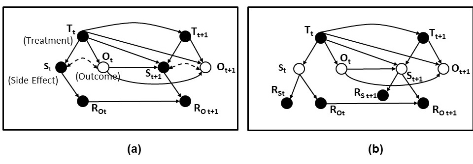
Figure 6: m-graphs depicting the problem of attrition. (a) MAR (b) MNAR

Example 8

Consider the m-graph in in figure 6 (a), where it is required to recover the causal effect of two sequential treatments, $T_{t}$ and $T_{t+1}$ on outcome $O_{t+1}$, namely
$P(O_{t+1}|do(T_{t},T_{t+1})$. This graph models a longitudinal study with attrition, where the $R$ variables represent subjects dropping out of the study due to side-effects $S_{t}$ and $S_{t+1}$ caused by the corresponding treatments (a practical problem discussed in Breskin et al. (2018); Cinelli and Pearl (2018)). The bi-directed arrows represent unmeasured health status indicating that participants with poor health are both more likely to experience side effects and incur unfavorable outcomes. Leveraging the exogeneity of the two treatments (rule 2 of do-calculus), we can remove the do-operator from the query expression, and obtain the identified estimand $P(O_{t+1}|do(T_{t},T_{t+1})=P(O_{t+1}|T_{t},T_{t+1})$. Since the parents of the $R$ variables are fully observed, the problem belongs to the MAR category, in which the joint distribution is recoverable (using corollary 2). Therefore $P(O_{t+1}|T_{t},T_{t+1})$ and hence our causal effect is also recoverable, and is given by: $\sum_{S_{t},S_{t+1}}P(O_{t+1}|T_{t},T_{t+1},S_{t},S_{t+1},R_{O_{t+1}}=0)P(S_{t},S_{t+1}|T_{t},T_{t+1})$.

Figure 6(b) represents a more intricate variant of the attrition problem, where the side effects themselves are partially observed and, worse yet, they cause their own missingness. Remarkably, the query is still recoverable, using Theorem 1 and the fact that, (i) $O_{t+1}$ is d-separated from both $R_{O_{t+1}}$ and $R_{O_{t}}$ given $(T_{t},T_{t+1},O_{t})$, and (ii) $O_{t}$ is d-separated from $R_{O_{t}}$ given $(T_{t},T_{t+1})$. The resulting estimand is: $\sum_{O_{t}}P(O_{t+1}|T_{t},T_{t+1},O_{t},R_{O_{t}}=0,R_{O_{t+1}}=0)P(O_{t}|R_{O_{t}}=0,T_{t},T_{t+1})$.

Figure 7(a) portrays another example of identifiable query, but in this case, the recoverability of the identified estimand is not obvious; constraint-based analysis (6.2) is needed to establish its recoverability.

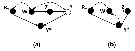
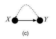
Figure 7: m-graphs in which (a) $P(y|do(z))$ is recoverable (b) $Y$ is treated as a latent variable and not explicitly portrayed. (c) bow-arc model in which causal effect of $X$ on $Y$ is non-identifiable.

Example 9

Examine the m-graph in figure 7(a). Suppose we are interested in the causal effect of Z (treatment) on outcome Y (death) where treatments are conditioned on (observed) X-rays report (W). Suppose that some unobserved factors (say quality of hospital equipment and staff) affect both attrition ($R_{y}$) and accuracy of test reports (W). In this setup the causal-effect query $P(y|do(z))$ is identifiable (by adjusting for W) through the estimand:

$$P(y|do(z)) =\sum_{w}P(y|z,w)P(w)$$ (7)

However, the factor $P(y|z,w)$ is not recoverable (by theorem 3), and one might be tempted to conclude that the causal effect is non-recoverable. We shall now show that it is nevertheless recoverable in three steps.

Recovering $P(y|do(z)$ given the m-graph in figure 7(a)

The first step is to transform the query (using the rules of do-calculus) into an equivalent expression such that no partially observed variables resides outside the do-operator.

$$P(y|do(z)) =P(y|do(z),R_{y}=0)\mbox{ (follows from rule 1 of do-calculus)}$$

$$=P(y^{*}|do(z),R_{y}=0)\mbox{ (using eq \ref{eq:miss1})}$$ (8)

The second step is to simplify the m-graph by removing superfluous variables, still retaining all relevant functional relationships. In our example $Y$ is irrelevant once we treating $Y^{*}$ as an outcome. The reduced m-graph is shown in figure 7(b). The third step is to apply the do-calculus (Pearl (2009b)) to the reduced graph (7(b)), and identify the modified query $P(y^{*}|do(z),R_{y}=0)$.

$$P(y^{*}|do(z),R_{y}=0) =\sum_{w}P(y^{*}|do(z),w,R_{y}=0)P(w|do(z),R_{y}=0)$$ (9)

$$P(y^{*}|do(z),w,R_{y}=0) =P(y^{*}|z,w,R_{y}=0)\mbox{ (by Rule-2 of do-calculus) }$$ (10)

$$P(w|do(z),R_{y}=0) =P(w|R_{y}=0)\mbox{ (by Rule-3 of do-calculus) })$$ (11)

Substituting (10) and (11) in (9) the causal effect becomes

$$P(y|do(z)) =\sum_{w}P(y^{*}|z,w,R_{y}=0)P(w|R_{y}=0)$$ (12)

which permits us to estimate our query from complete cases only. While in this case we were able to recover the causal effect using one pass over the three steps, in more complex cases we might need to repeatedly apply these steps in order to recover the query.

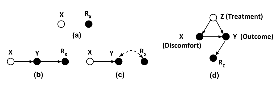
Figure 8: (a) m-graph with an untestable claim: $Z\mbox{$\bot\!\!\!\bot$}R_{z}|X,Y$, (b) & (c) Two statistically indistinguishable models, (d) m-graph depicting MCAR.

4 Testability Under Missingness

In this section we seek ways to detect mis-specifications of the missingness model. While discussing testability, one must note a phenomenon that recurs in missing data analysis: Not all that looks testable is testable. Specifically, although every d-separation in the graph implies conditional independence in the recovered distribution, some of those independencies are imposed by construction, in order to satisfy the model’s claims, and these do not provide means of refuting the model. We exemplify this peculiarity below.

Example 10

Consider the m-graph in figure 8(a). It is evident that the problem is MCAR (definition in section 4.2). Hence $P(X,R_{x})$ is recoverable. The only conditional independence embodied in the graph is $X\mbox{$\bot\!\!\!\bot$}R_{x}$. At first glance it might seem as if $X\mbox{$\bot\!\!\!\bot$}R_{x}$ is testable since we can go to the recovered distribution and check whether it satisfies this conditional independence. However, $X\mbox{$\bot\!\!\!\bot$}R_{x}$ will always be satisfied in the recovered distribution, because it was recovered so as to satisfy $X\mbox{$\bot\!\!\!\bot$}R_{x}$. This can be shown explicitly as follows:

$$P(X,R_{x}) =P(X|R_{x})P(R_{x})$$

$$=P(X|R_{x}=0)P(R_{x})\mbox{ (Using $X\mbox{$\bot\!\!\!\bot$}R_{x}$)}$$

$$=P(X^{*}|R_{x}=0)P(R_{x})\mbox{( Using Equation \ref{eq:miss1})}$$

Likewise,

$$P(X)P(R_{x}) =P(X^{*}|R_{x}=0)P(R_{x})$$

Therefore, the claim, $X\mbox{$\bot\!\!\!\bot$}R_{x}$, cannot be refuted by any recovered distribution, regardless of what process actually generated the data. In other words, any data whatsoever with $X$ partially observed can be made compatible with the model postulated.

The following theorem characterizes a more general class of untestable claims.

Theorem 4 (Mohan and Pearl (2014b))

Let $\{Z,X\}\subseteq V_{m}$ and $W\subseteq V_{o}$. Conditional independencies of the form $X\mbox{$\bot\!\!\!\bot$}R_{x}|Z,W,R_{z}$ are untestable.

The preceding example demonstrates this theorem as a special case, with $Z=W=R_{z}=\emptyset$. The next section provides criteria for testable claims.

4.1 Graphical Criteria for Testability

The criterion for detecting testable implications reads as follows: A d-separation condition displayed in the graph is testable if the R variables associated with all the partially observed variables in it are either present in the separating set or can be added to the separating set without spoiling the separation. The following theorem formally states this criterion using three syntactic rules (Mohan and Pearl (2014b)).

Theorem 5

A sufficient condition for an m-graph to be testable is that it encodes one of the following types of independences:

$$X\mbox{$\bot\!\!\!\bot$}Y|Z,R_{x},R_{y},R_{z}$$ (13)

$$X\mbox{$\bot\!\!\!\bot$}R_{y}|Z,R_{x},R_{z}$$ (14)

$$R_{x}\mbox{$\bot\!\!\!\bot$}R_{y}|Z,R_{z}$$ (15)

In words, any d-separation that can be expressed in the format stated above is testable. It is understood that, if $X$ or $Y$ or $Z$ are fully observed, the corresponding $R$ variables may be removed from the conditioning set. Clearly, any conditional independence comprised exclusively of fully observed variables is testable. To search for such refutable claims, one needs to only examine the missing edges in the graph and check whether any of its associated set of separating sets satisfy the syntatctic format above.

To illustrate the power of the criterion we present the following example.

Example 11

Examine the m-graph in figure 8 (d). The missing edges between $Z$ and $R_{z}$, and $X$ and $R_{z}$ correspond to the conditional independencies: $Z\mbox{$\bot\!\!\!\bot$}R_{z}|(X,Y)$ and $X\mbox{$\bot\!\!\!\bot$}R_{z}|Y$, respectively. The former is untestable (following theorem 4) while the latter is testable, since it complies with (14) in theorem 5.

4.1.1 Tests Corresponding to the Independence Statements in Theorem 5

A testable claim needs to be expressed in terms of proxy variables before it can be operationalized. For example, a specific instance of the claim $X\mbox{$\bot\!\!\!\bot$}Y|Z,R_{x},R_{y},R_{z}$, when $R_{x}=0,R_{y}=0,R_{z}=0$ gives $X\mbox{$\bot\!\!\!\bot$}Y|Z,R_{x}=0,R_{y}=0,R_{z}=0$. On rewriting this claim as an equation and applying equation 1 we get,

$$P(X^{*}|Z^{*},R_{x}=0,R_{y}=0,R_{z}=0) =P(X^{*}|Y^{*},Z^{*},R_{x}=0,R_{y}=0,R_{z}=0)$$

This equation exclusively comprises of observed quantities and can be directly tested given the input distribution: $P(X^{*},Y^{*},Z^{*},R_{x},R_{y},R_{z})$. Finite sample techniques for testing conditional independencies are cited in the next section. In a similar manner we can devise tests for the remaining two statements in theorem 5.

The tests corresponding to the three independence statements in theorem 5 are:

• $P(X^{*}|Z^{*},R_{x}=0,R_{y}=0,R_{z}=0)=P(X^{*}|Y^{*},Z^{*},R_{x}=0,R_{y}=0,R_{z}=0)$,

• $P(X^{*}|Z^{*},R_{x}=0,R_{z}=0)=P(X^{*}|R_{y},Z^{*},R_{x}=0,R_{z}=0)$

• $P(R_{x}|Z^{*},R_{z}=0)=P(R_{x}|R_{y},Z^{*},R_{z}=0)$

The next section specializes these results to the classes of MAR and MCAR problems which have been given some attention in the existing literature.

4.2 Testability of MCAR and MAR

A chi square based test for MCAR was proposed by Little (1988) in which a high value falsified MCAR(Rubin, 1976). Rubin-MAR is known to be untestable (Allison, 2002). Potthoff et al. (2006) defined MAR at the variable-level (identical to that in section 2.2) and showed that it can be tested. Theorem 6, given below presents stronger conditions under which a given MAR model is testable (Mohan and Pearl (2014b)). Moreover, it provides diagnostic insight in case the test is violated. We further note that these conditional independence tests may be implemented in practice using different techniques such as G-test, chi square test, testing for zero partial correlations or by tests such as those described in Székely et al. (2007); Gretton et al. (2012); Sriperumbudur et al. (2010).

Theorem 6 (MAR is Testable)

Given that $|V_{m}|>0$, $V_{m}\mbox{$\bot\!\!\!\bot$}R|V_{o}$ is testable if and only if $|V_{m}|>1$ i.e. $|V_{m}|$ is not a singleton set.

In words, given a dataset with two or more partially observed variables, it is always possible to test whether MAR holds. We exemplify such tests below.

Example 12 (Tests for MAR)

Given a dataset where $V_{m}=\{A,B\}$ and $V_{o}=\{C\}$, the MAR condition states that $(A,B)\mbox{$\bot\!\!\!\bot$}(R_{A},R_{B})|C$. This statement implies the following two statements which match syntactic criteria in 14 and hence are testable.

1. $A\mbox{$\bot\!\!\!\bot$}R_{B}|C,R_{A}$

2. $B\mbox{$\bot\!\!\!\bot$}R_{A}|C,R_{B}$

The testable implication corresponding to (1) and (2) above are the following:

$$P(A^{*},R_{B}|C,R_{A}=0) =P(A^{*}|C,R_{A}=0)P(R_{B}|C,R_{A}=0)$$

$$P(B^{*},R_{A}|C,R_{B}=0) =P(B^{*}|C,R_{B}=0)P(R_{A}|C,R_{B}=0)$$

While refutation of these tests immediately imply that the data are not MAR, we can never verify the MAR condition. However if MAR is refuted, it is possible to pinpoint and locate the source of error in the model. For instance, if claim (1) is refuted then one should consider adding an edge between $A$ and $R_{B}$.

Remark 3

A recent paper by I Bojinov, N Pillai and D Rubin (Bojinov et al., 2017) has adopted some of the aforementioned tests for MAR models, and demonstrated their use on simulated data. Their paper is a testament to the significance and applicability of our results (specifically, section 3.1 and 6 in [36] to real world problems.

Corollary 3 (MCAR is Testable)

Given that $|V_{m}|>0$, $(V_{m},V_{O})\mbox{$\bot\!\!\!\bot$}R|V_{o}$ is testable if and only if $|V_{m}|+|V_{O}|\geq 2$.

Example 13 (Tests for MCAR)

Given a dataset where $V_{m}=\{A,B\}$ and $V_{o}=\{C\}$, the MCAR condition states that $(A,B,C)\mbox{$\bot\!\!\!\bot$}(R_{A},R_{B})$. This statement implies the following statements which match syntactic criteria in 14 and 13 and hence are testable.

1. $A\mbox{$\bot\!\!\!\bot$}R_{B}|R_{A}$

2. $B\mbox{$\bot\!\!\!\bot$}R_{A}|R_{B}$

3. $C\mbox{$\bot\!\!\!\bot$}R_{A}$

The testable implication corresponding to (1) and (2) above are the following:

$$P(A^{*},R_{B}|C,R_{A}=0) =P(A^{*}|C,R_{A}=0)P(R_{B}|C,R_{A}=0)$$

$$P(B^{*},R_{A}|C,R_{B}=0) =P(B^{*}|C,R_{B}=0)P(R_{A}|C,R_{B}=0)$$

$$P(C,R_{A}) =P(C)P(R_{A})$$

4.3 On the Causal Nature of the Missing Data Problem

Examine the m-graphs in Figure 8(b) and (c). $X\mbox{$\bot\!\!\!\bot$}R_{x}|Y$ and $X\mbox{$\bot\!\!\!\bot$}R_{x}$ are the conditional independence statements embodied in models 8(b) and (c), respectively. Neither of these statements are testable. Therefore they are statistically indistinguishable. However, notice that $P(XY)$ is recoverable in figure 8(b) but not in figure 8(c) implying that,

• No universal algorithm exists that can decide if a query is recoverable or not without looking at the model.

Further notice that $P(X)$ is recoverable in both models albeit using two different methods. In model 8(b) we have $P(X)=\sum_{Y}P(X^{*}|Y,R_{x}=0)P(y)$ and in model 8(c) we have $P(X)=P(X^{*}|R_{x}=0)$. This leads to the conclusion that,

• No universal algorithm exists that can produce a consistent estimate whenever such exists.

The impossibility of determining from statistical assumptions alone, (i) whether a query is recoverable and (ii) how the query is to be recovered, if it is recoverable, attests to the causal nature of the missing data problem. Although Rubin (1976) alludes to the causal aspect of this problem, subsequent research has treated missing data mostly as a statistical problem. A closer examination of the testability and recovery conditions shows however that a more appropriate perspective would be to treat missing data as a causal inference problem.

5 Conclusions

All methods of missing data analysis rely on assumptions regarding the reasons for missingness. Casting these assumptions in a graphical model, permits researchers to benefit from the inherent transparency of such models as well as their ability to explicate the statistical implication of the underlying assumptions in terms of conditional independence relations among observed and partially observed variables. We have shown that these features of graphical models can be harnessed to study unchartered territories of missing data research. In particular, we charted the estimability of statistical and causal parameters in broad classes of MNAR problems, and the testability of the model assumptions under missingness conditions.

An important feature of our analysis is its query dependence. In other words, while certain properties of the underlying distribution may be deemed unrecoverable, others can be proven to be recoverable, and by smart estimation algorithms.

We should emphasize that all our results assume non parametric models. In other words, no assumptions are needed about the functional or distributional nature of the relationships involved.

In light of our findings we question the benefits of the traditional taxonomy that classifies missingness problems into MCAR, MAR and MNAR. To decide if a problem falls into any of these categories a user must have a model of the causes of missingness and once this model is articulated the criteria we have derived for recoverability and testability can be readily applied. Hence we see no need to refine and elaborate conditions for MAR.

The testability criteria derived in this paper can be used not only to rule out misspecified models but also to locate specific mis-specifications for the purpose of model updating and re-specification. More importantly, we have shown that it is possible to determine if and how a target quantity is recoverable, even in models where missingness is not ignorable. Finally, knowing which sub-structures in the graph prevent recoverability can guide data collection procedures by identifying auxiliary variables that need to be measured to ensure recovery, or problematic variables that may compromise recovery if measured imprecisely.

6 Appendix

6.1 Estimation when the Data May not be Missing at Random. (Little and Rubin (2014), page-22)

Essentially all the literature on multivariate incomplete data assumes that the data are MAR, and much of it also assumes that the data are MCAR. Chapter 15 deals explicitly with the case when the data are not MAR, and models are needed for the missing-data mechanism. Since it is rarely feasible to estimate the mechanism with any degree of confidence, the main thrust of these methods is to conduct sensitivity analyses to assess the effect of alternative assumptions about the missing-data mechanism.

6.2 A Complex Example of Recoverability

We use $R=0$ as a shorthand for the event where all variables are observed i.e. $R_{V_{m}}=0$.

Example 14

Given the m-graph in figure 5 (c), we will now recover the joint distribution.

$$P(W,X,Y,Z) =P(W,X,Y,Z)\frac{P(W,X,Y,Z,R=0)}{P(W,X,Y,Z,R=0)}=\frac{P(W,X,Y,Z,R=0)}{P(R=0|W,X,Y,Z)}$$

Factorization of the denominator based on topological ordering of $$R$$ variables yields,

$$P(W,X,Y,Z) =\frac{P(W,X,Y,Z,R=0)}{P(R_{y}=0|W,X,Y,Z,R_{x}=0,R_{w}=0,R_{z}=0)P(R_{x}=0|W,X,Y,Z,R_{w}=0,R_{z}=0)}$$

$$\hskip 142.26378pt\frac{1}{P(R_{w}=0|W,X,Y,Z,R_{z}=0)P(R_{z}=0|W,X,Y,Z)}$$

On simplifying each factor of the form: $$P(R_{a}=0|B) B_{1}\in B R_{a}\mbox{$\bot\!\!\!\bot$}B_{1}|B-B_{1}$$, by removing from it all such that , we get:

$$P(W,X,Y,Z) =\frac{P(W,X,Y,Z,R=0)}{P(R_{z}=0)P(R_{w}=0|Z)P(R_{y}=0|X,W,R_{x}=0)P(R_{x}=0|Y,W)}$$ (16)

$P(WXYZ)$ is recoverable if all factors in the preceding equation is recoverable. Examining each factor one by one we get:

• $P(W,X,Y,Z,R=0)$: Recoverable as $P(W^{*},X^{*},Y^{*},Z^{*},R=0)$ using equation 1.

• $P(R_{z}=0)$: Directly estimable from the observed-data distribution.

• $P(R_{w}=0|Z)$: Recoverable as $P(R_{w}=0|Z^{*},R_{z}=0)$, using $R_{w}\mbox{$\bot\!\!\!\bot$}R_{z}|Z$ and equation 1.

• $P(R_{y}=0|X,W,R_{x}=0)$: Recoverable as $P(R_{y}=0|X^{*},W^{*},R_{x}=0,R_{w}=0)$, using $R_{y}\mbox{$\bot\!\!\!\bot$}R_{w}|X,W,R_{x}$ and equation 1.

• $P(R_{x}=0|Y,W)$: The procedure for recovering $P(R_{x}=0|Y,W)$ is rather involved and requires converting the probabilistic sub-query to a causal one as detailed below.

$$P(R_{x}=0|Y,W=w) =P(R_{x}=0|Y,do(W=w))\mbox{(Rule-2 of do calculus)}$$

$$=\frac{P(R_{x}=0|Y,R_{y}=0,do(w))}{P(R_{x}=0|Y,R_{y}=0,do(w))}P(R_{x}=0|Y,do(W=w))$$

$$=P(R_{x}=0|Y,R_{y}=0,do(w))\frac{P(R_{y}=0|Y,do(w))}{P(R_{y}=0|Y,do(w),R_{x}=0)}$$ (17)

To prove recoverability of $P(R_{x}=0|Y,W=w)$, we have to show that all factors in equation 17 are recoverable.

Recovering $\mathbf{P(R_{y}=0|Y,do(w),R_{x}=0):}$

Observe that $P(R_{y}=0|Y,do(w),R_{x}=0)=P(R_{y}=0|do(w),R_{x}=0)$ by Rule-1 of do calculus. To recover $P(R_{y}=0|do(w),R_{x}=0)$ it is sufficient to show that $P(X^{*},Y^{*},R_{x},R_{y},Z|do(w))$ is recoverable in $G^{\prime}$, the latent structure corresponding to $G$ in which $X$ and $Y$ are treated as latent variables.

$$P(X^{*},Y^{*},R_{x},R_{y},Z|do(w)) =P(X^{*},Y^{*},R_{x},R_{y}|Z,do(w))P(Z|do(w))$$

$$=P(X^{*},Y^{*},R_{x},R_{y}|Z,w)P(Z|do(w))\mbox{ (Rule-2 of do-calculus)}$$

$$=P(X^{*},Y^{*},R_{x},R_{y}|Z,w)P(Z)\mbox{ (Rule-3 of do-calculus)}$$

Using $$(X^{*},Y^{*},R_{x},R_{y})\mbox{$\bot\!\!\!\bot$}(R_{z},R_{w})|(Z,W) Z\mbox{$\bot\!\!\!\bot$}R_{z}$$, equation 1 and we show that the causal effect is recoverable as:

$$P(X^{*},Y^{*},R_{x},R_{y},Z|do(w)) =P(X^{*},Y^{*},R_{x},R_{y}|Z^{*},w^{*},R_{w}=0,R_{z}=0)P(Z^{*}|R_{z}=0)$$ (18)

Recovering $\mathbf{P(R_{x}=0|Y,do(w),R_{y}=0):}$

Using equation 1, we can rewrite $P(R_{x}=0|Y,do(w),R_{y}=0)$ as $P(R_{x}=0|Y^{*},do(w),R_{y}=0)$. Its recoverability follows from equation 18.

Recovering $\mathbf{P(R_{y}=0|Y,do(w)):}$

$$P(R_{y}=0|Y,do(w)) =\frac{P(R_{y}=0,Y|do(w))}{\sum_{R_{x}}P(R_{y}=0,Y,R_{x}|do(w))+P(R_{y}=1,Y,R_{x}|do(w))}$$

$$=\frac{P(R_{y}=0,Y^{*}|do(w))}{\sum_{R_{x}}P(R_{y}=0,Y^{*},R_{x}|do(w))+P(R_{y}=1,Y,R_{x}|do(w))}\mbox{(using eq \ref{eq:miss1})}$$

$$P(R_{y}=0,Y^{*}|do(w)) P(R_{y}=0,Y^{*},R_{x}|do(w)) P(R_{y}=1,Y^{*},R_{x}|do(w))$$ and are recoverable from equation 18. We will now show that is recoverable as well.

$$P(R_{y}=1,Y,R_{x}|do(w)) =\frac{P(R_{y}=0,Y,R_{x}|do(w))}{P(R_{y}=0|R_{x},Y|do(w))}-P(R_{y}=0,R_{x},Y|do(w))$$

Using equation 1 and Rule-1 of do-calculus we get,

$$=\frac{P(R_{y}=0,Y^{*},R_{x}|do(w))}{P(R_{y}=0|R_{x},do(w))}-P(R_{y}=0,R_{x},Y^{*}|do(w))$$

Each factor in the preceding equation is estimable from equation 18. Hence $$P(R_{y}=1,Y,R_{x},do(w)) P(R_{y}=0|Y,do(w))$$ and therefore, is recoverable.

Since all factors in equation 17 are recoverable, joint distribution is recoverable.

References

- Adams (2007) Adams, J. (2007). Researching complementary and alternative medicine. Routledge.
- Allison (2002) Allison, P. (2002). Missing data series: Quantitative applications in the social sciences.
- Allison (2003) Allison, P. D. (2003). Missing data techniques for structural equation modeling. Journal of abnormal psychology 112(4), 545.
- Balakrishnan (2010) Balakrishnan, N. (2010). Methods and applications of statistics in the life and health sciences. John Wiley & Sons.
- Bang and Robins (2005) Bang, H. and J. M. Robins (2005). Doubly robust estimation in missing data and causal inference models. Biometrics 61(4), 962–973.
- Bartlett et al. (2014) Bartlett, J. W., J. R. Carpenter, K. Tilling, and S. Vansteelandt (2014). Improving upon the efficiency of complete case analysis when covariates are mnar. Biostatistics 15(4), 719–730.
- Bartlett et al. (2015) Bartlett, J. W., O. Harel, and J. R. Carpenter (2015). Asymptotically unbiased estimation of exposure odds ratios in complete records logistic regression. American journal of epidemiology 182(8), 730–736.
- Bojinov et al. (2017) Bojinov, I., N. Pillai, and D. Rubin (2017). Diagnosing missing always at random in multivariate data. arXiv preprint arXiv:1710.06891.
- Breskin et al. (2018) Breskin, A., S. R. Cole, and M. G. Hudgens (2018). A practical example demonstrating the utility of single-world intervention graphs. Epidemiology 29(3), e20–e21.
- Carpenter and Kenward (2014) Carpenter, J. and M. Kenward (2014). Missing data in randomised controlled trials–a practical guide. 2007. Published at: http://www. pcpoh. bham. ac. uk/publichealth/nccrm/PDFs_and_documents/Publications/Final_Report_RM04_JH17_mk. pdf.
- Chang (2011) Chang, M. (2011). Modern issues and methods in biostatistics. Springer Science & Business Media.
- Cinelli and Pearl (2018) Cinelli, C. and J. Pearl (2018). On the utility of causal diagrams in modeling attrition: a practical example. Technical Report R-479, http://ftp.cs.ucla.edu/pub/stat_ser/r479.pdf, Department of Computer Science, University of California, Los Angeles, CA. Forthcoming, Journal of Epidemiology.
- Collins et al. (2001) Collins, L. M., J. L. Schafer, and C.-M. Kam (2001). A comparison of inclusive and restrictive strategies in modern missing data procedures. Psychological methods 6(4), 330.
- Daniel et al. (2012) Daniel, R. M., M. G. Kenward, S. N. Cousens, and B. L. De Stavola (2012). Using causal diagrams to guide analysis in missing data problems. Statistical methods in medical research 21(3), 243–256.
- Darwiche (2009) Darwiche, A. (2009). Modeling and reasoning with Bayesian networks. Cambridge University Press.
- Dempster et al. (1977) Dempster, A., N. Laird, and D. Rubin (1977). Maximum likelihood from incomplete data via the em algorithm. Journal of the Royal Statistical Society. Series B (Methodological), 1–38.
- Doretti et al. (2018) Doretti, M., S. Geneletti, and E. Stanghellini (2018). Missing data: a unified taxonomy guided by conditional independence. International Statistical Review 86(2), 189–204.
- Elwert (2013) Elwert, F. (2013). Graphical causal models. In Handbook of causal analysis for social research, pp. 245–273. Springer.
- Fitzmaurice et al. (2008) Fitzmaurice, G., G. Molenberghs, M. Davidian, and G. Verbeke (2008). Generalized estimating equations for longitudinal data analysis. In Longitudinal data analysis, pp. 51–86. Chapman and Hall/CRC.
- Gill and Robins (1997) Gill, R. D. and J. M. Robins (1997). Sequential models for coarsening and missingness. In Proceedings of the First Seattle Symposium in Biostatistics, pp. 295–305. Springer.
- Gill et al. (1997) Gill, R. D., M. J. Van Der Laan, and J. M. Robins (1997). Coarsening at random: Characterizations, conjectures, counter-examples. In Proceedings of the First Seattle Symposium in Biostatistics, pp. 255–294. Springer.
- Gleason and Staelin (1975) Gleason, T. C. and R. Staelin (1975). A proposal for handling missing data. Psychometrika 40(2), 229–252.
- Graham (2012) Graham, J. (2012). Missing Data: Analysis and Design (Statistics for Social and Behavioral Sciences). Springer.
- Graham (2009) Graham, J. W. (2009). Missing data analysis: Making it work in the real world. Annual review of psychology 60, 549–576.
- Greenland and Pearl (2011) Greenland, S. and J. Pearl (2011). Causal diagrams. In International encyclopedia of statistical science, pp. 208–216. Springer.
- Gretton et al. (2012) Gretton, A., K. M. Borgwardt, M. J. Rasch, B. Schölkopf, and A. Smola (2012). A kernel two-sample test. Journal of Machine Learning Research 13(Mar), 723–773.
- Haitovsky (1968) Haitovsky, Y. (1968). Missing data in regression analysis. Journal of the Royal Statistical Society. Series B (Methodological), 67–82.
- Holmes et al. (2018) Holmes, C. B., I. Sikazwe, K. Sikombe, I. Eshun-Wilson, N. Czaicki, L. K. Beres, N. Mukamba, S. Simbeza, C. B. Moore, C. Hantuba, et al. (2018). Estimated mortality on hiv treatment among active patients and patients lost to follow-up in 4 provinces of zambia: Findings from a multistage sampling-based survey. PLoS medicine 15(1), e1002489.
- Huang and Valtorta (2006) Huang, Y. and M. Valtorta (2006). Identifiability in causal bayesian networks: A sound and complete algorithm. In Proceedings of the National Conference on Artificial Intelligence, Volume 21, pp. 1149. Menlo Park, CA; Cambridge, MA; London; AAAI Press; MIT Press; 1999.
- Koller and Friedman (2009) Koller, D. and N. Friedman (2009). Probabilistic graphical models: principles and techniques.
- Kuroki and Pearl (2014) Kuroki, M. and J. Pearl (2014). Measurement bias and effect restoration in causal inference. Biometrika 101(2), 423–437.
- Lauritzen (2001) Lauritzen, S. L. (2001). Causal inference from graphical models. Complex stochastic systems, 63–107.
- Li et al. (2013) Li, L., C. Shen, X. Li, and J. M. Robins (2013). On weighting approaches for missing data. Statistical methods in medical research 22(1), 14–30.
- Little and Rubin (2002) Little, R. and D. Rubin (2002). Statistical analysis with missing data. Wiley.
- Little and Rubin (2014) Little, R. and D. Rubin (2014). Statistical analysis with missing data. John Wiley & Sons. ISBN:9781118625880.
- Little (1988) Little, R. J. (1988). A test of missing completely at random for multivariate data with missing values. Journal of the American Statistical Association 83(404), 1198–1202.
- Meyers et al. (2006) Meyers, L. S., G. Gamst, and A. J. Guarino (2006). Applied multivariate research: Design and interpretation. Sage.
- Mohan (2018) Mohan, K. (2018). On handling self-masking and other hard missing data problems. AAAI Symposium 2018, https://why19.causalai.net/papers/mohan-why19.pdf.
- Mohan and Pearl (2014a) Mohan, K. and J. Pearl (2014a). Graphical models for recovering probabilistic and causal queries from missing data. In Z. Ghahramani, M. Welling, C. Cortes, N. Lawrence, and K. Weinberger (Eds.), Advances in Neural Information Processing Systems 27, pp. 1520–1528. Curran Associates, Inc.
- Mohan and Pearl (2014b) Mohan, K. and J. Pearl (2014b). On the testability of models with missing data. Proceedings of AISTAT.
- Mohan et al. (2013) Mohan, K., J. Pearl, and J. Tian (2013). Graphical models for inference with missing data. In Advances in Neural Information Processing Systems 26, pp. 1277–1285.
- Mohan et al. (2014) Mohan, K., G. Van den Broeck, A. Choi, and J. Pearl (2014). An efficient method for bayesian network parameter learning from incomplete data. Technical report, UCLA. Presented at Causal Modeling and Machine learning Workshop, ICML-2014.
- Osborne (2012) Osborne, J. W. (2012). Best practices in data cleaning: A complete guide to everything you need to do before and after collecting your data. Sage Publications.
- Osborne (2014) Osborne, J. W. (2014). Best practices in logistic regression. SAGE Publications.
- Pearl (1988) Pearl, J. (1988). Probabilistic reasoning in intelligent systems: networks of plausible inference. Morgan Kaufmann.
- Pearl (2009a) Pearl, J. (2009a). Causal inference in statistics: An overview. Statistics Surveys 3, 96–146.
- Pearl (2009b) Pearl, J. (2009b). Causality: models, reasoning and inference. Cambridge Univ Press, New York.
- Pearl and Bareinboim (2014) Pearl, J. and E. Bareinboim (2014). External validity: From do-calculus to transportability across populations. Statistical Science 29(4), 579–595.
- Peters and Enders (2002) Peters, C. L. O. and C. Enders (2002). A primer for the estimation of structural equation models in the presence of missing data: Maximum likelihood algorithms. Journal of Targeting, Measurement and Analysis for Marketing 11(1), 81–95.
- Pfeffermann and Sikov (2011) Pfeffermann, D. and A. Sikov (2011, 06). Imputation and estimation under nonignorable nonresponse in household surveys with missing covariate information. Journal of Official Statistics 27.
- Potthoff et al. (2006) Potthoff, R., G. Tudor, K. Pieper, and V. Hasselblad (2006). Can one assess whether missing data are missing at random in medical studies? Statistical methods in medical research 15(3), 213–234.
- Resseguier et al. (2011) Resseguier, N., R. Giorgi, and X. Paoletti (2011). Sensitivity analysis when data are missing not-at-random. Epidemiology 22(2), 282.
- Rhoads (2012) Rhoads, C. H. (2012). Problems with tests of the missingness mechanism in quantitative policy studies. Statistics, Politics, and Policy 3(1).
- Robins (1997) Robins, J. M. (1997). Non-response models for the analysis of non-monotone non-ignorable missing data. Statistics in Medicine 16(1), 21–37.
- Robins (2000) Robins, J. M. (2000). Robust estimation in sequentially ignorable missing data and causal inference models. In Proceedings of the American Statistical Association, Volume 1999, pp. 6–10. Indianapolis, IN.
- Robins et al. (2000) Robins, J. M., A. Rotnitzky, and D. O. Scharfstein (2000). Sensitivity analysis for selection bias and unmeasured confounding in missing data and causal inference models. In Statistical models in epidemiology, the environment, and clinical trials, pp. 1–94. Springer.
- Robins et al. (1994) Robins, J. M., A. Rotnitzky, and L. P. Zhao (1994). Estimation of regression coefficients when some regressors are not always observed. Journal of the American statistical Association 89(427), 846–866.
- Rotnitzky et al. (1998) Rotnitzky, A., J. M. Robins, and D. O. Scharfstein (1998). Semiparametric regression for repeated outcomes with nonignorable nonresponse. Journal of the american statistical association 93(444), 1321–1339.
- Rubin (1976) Rubin, D. (1976). Inference and missing data. Biometrika 63, 581–592.
- Rubin (1978) Rubin, D. B. (1978). Multiple imputations in sample surveys-a phenomenological bayesian approach to nonresponse. In Proceedings of the survey research methods section of the American Statistical Association, Volume 1, pp. 20–34. American Statistical Association.
- Scharfstein et al. (1999) Scharfstein, D. O., A. Rotnitzky, and J. M. Robins (1999). Adjusting for nonignorable drop-out using semiparametric nonresponse models. Journal of the American Statistical Association 94(448), 1096–1120.
- Scheffer (2002) Scheffer, J. (2002). Dealing with missing data. Research Letters in the Information and Mathematical Sciences, 153–160.
- Seaman et al. (2013) Seaman, S., J. Galati, D. Jackson, J. Carlin, et al. (2013). What is meant by “missing at random”? Statistical Science 28(2), 257–268.
- Shpitser and Pearl (2006) Shpitser, I. and J. Pearl (2006). Identification of conditional interventional distributions. In Proceedings of the Twenty-Second Conference on Uncertainty in Artificial Intelligence, pp. 437–444.
- Sriperumbudur et al. (2010) Sriperumbudur, B. K., A. Gretton, K. Fukumizu, B. Schölkopf, and G. R. Lanckriet (2010). Hilbert space embeddings and metrics on probability measures. Journal of Machine Learning Research 11(Apr), 1517–1561.
- Sverdlov (2015) Sverdlov, O. (2015). Modern adaptive randomized clinical trials: statistical and practical aspects. Chapman and Hall/CRC.
- Székely et al. (2007) Székely, G. J., M. L. Rizzo, N. K. Bakirov, et al. (2007). Measuring and testing dependence by correlation of distances. The annals of statistics 35(6), 2769–2794.
- Thoemmes and Mohan (2015) Thoemmes, F. and K. Mohan (2015). Graphical representation of missing data problems. Structural Equation Modeling: A Multidisciplinary Journal.
- Thoemmes and Rose (2013) Thoemmes, F. and N. Rose (2013). Selection of auxiliary variables in missing data problems: Not all auxiliary variables are created equal. Technical Report R-002, Cornell University.
- Tian and Pearl (2002) Tian, J. and J. Pearl (2002). On the testable implications of causal models with hidden variables. In Proceedings of the Eighteenth conference on Uncertainty in artificial intelligence, pp. 519–527. Morgan Kaufmann Publishers Inc.
- Van den Broeck et al. (2015) Van den Broeck, G., K. Mohan, A. Choi, A. Darwiche, and J. Pearl (2015). Efficient algorithms for bayesian network parameter learning from incomplete data. In Proceedings of the Thirty-First Conference on Uncertainty in Artificial Intelligence, pp. 161–170.
- van Stein and Kowalczyk (2016) van Stein, B. and W. Kowalczyk (2016). An incremental algorithm for repairing training sets with missing values. In International Conference on Information Processing and Management of Uncertainty in Knowledge-Based Systems, pp. 175–186. Springer.
- Verma and Pearl (1991) Verma, T. and J. Pearl (1991). Equivalence and synthesis of causal models. In Proceedings of the Sixth Conference in Artificial Intelligence, pp. 220–227. Association for Uncertainty in AI.
- White and Carlin (2010) White, I. R. and J. B. Carlin (2010). Bias and efficiency of multiple imputation compared with complete-case analysis for missing covariate values. Statistics in medicine 29(28), 2920–2931.
- Zhang et al. (2016) Zhang, N., H. Chen, and M. R. Elliott (2016). Nonrespondent subsample multiple imputation in two-phase sampling for nonresponse. Journal of Official Statistics 32(3), 769–785.