Channel surface plasmons in a continuous and flat graphene sheet

Abstract

We derive an integral equation describing surface-plasmon polaritons in graphene deposited on a substrate with a planar surface and a dielectric protrusion in the opposite surface of the dielectric slab. We show that the problem is mathematically equivalent to the solution of a Fredholm equation, which we solve exactly. In addition, we show that the dispersion relation of the channel surface plasmons is determined by the geometric parameters of the protrusion alone. We also show that such system supports both even and odd modes. We give the electrostatic potential and the intensity plot of the electrostatic field, which clearly show the transverse localized nature of the surface plasmons in a continuous and flat graphene sheet.

I Introduction

Light-matter interaction at the nanoscale is the realm of plasmonics. In the visible and near-IR spectral range one generally relies on the plasmonic properties of noble metals, such as Gold, Silver, and Copper. On the other hand, in the mid-infrared (IR) and in the THz the use of noble metals is excluded due to poor confinement of the surface plasmons. It is in this context that graphene emerges as a platform for plasmonics in the mid-IR and in the THz spectral range, since this material supports strongly confined surface plasmons in this frequency region Ju et al. (2011); Yan et al. (2012).

In the field of plasmonics one can distinguish between two different types of surface plasmons. For graphene, as for noble metals, the types are: (i) surface-plasmon polaritons and (ii) localized surface plasmons. The former are propagating surface waves on the graphene surface, whereas the latter are localized excitations in graphene nanostructures, such as ribbons Ju et al. (2011) and disksYan et al. (2012). Thus, in general, for obtaining localized plasmons in graphene one has to pattern the graphene sheet, which hinders the quality factor of these excitations. It would be, therefore, convenient, to provide a method to induce localized plasmons in a continuous graphene sheet. To investigate this possibility is the purpose of this paper, where we should the existence of transversely localized channel plasmons.

The coupled mode of an electromagnetic field with charge density oscillations of a conductor is called surface plasmon-polaritons (SPP). The synthesis of graphene and other new two dimensional (2D) materials opened the door to natural candidates to support this type of surface modes, therefore creating a new field inside plasmonics Gonçalves and Peres (2016); Basov et al. (2016); Low et al. (2017). The most interesting properties of the SPP are the confinement of light below the diffraction limit Atwater (2007). The list of applications for SPP is extensive, including biochemical sensing Brolo (2012); Acimovic et al. (2014); Rodrigo et al. (2015), solar cells Green and Pillai (2012), optical tweezers Reece (2008); Juan et al. (2011), and transformation optics Huidobro et al. (2010); Pendry et al. (2012). In planar dielectric-metal interfaces, the SPP is confined along the direction transverse to the surface. However, at dielectric gaps, such as V-shaped groove and nanogaps, such plasmons can be also be confined along the non translational-invariant direction, being classified as channel plasmon-polaritons (CPP) Smith et al. (2015). Those systems can be used to steer SPP, thus forming plasmonic waveguides Nielsen et al. (2008); Gramotnev and Pile (2004).

Inside the sub-field of 2D photonics, graphene attracted much attention due to its unique properties, including the fact that its optical properties can be controlled externaly by electrostatic gating, originating long-lived plasmons, with large field confinement in the THz and mid-IR spectral range Jablan et al. (2009); Tassin et al. (2012); Wenger et al. (2016); Gonçalves and Peres (2016); Xiao et al. (2016); García de Abajo (2014). On the other hand, there are few studies on CPP in graphene. The existing ones discuss 2D nano-slitsGonçalves et al. (2017a) and covered grooves and wedges Liu et al. (2013); Smirnova et al. (2016); Gonçalves et al. (2017b). In all these approaches graphene is deposited in a deformed substrate, thus assuming the same shape of the substrate. This approaches reduce the quality factor of the SPP. Therefore it would be ideal to find a method where a continuous graphene sheet is deposited on a flat substrate but would still support localized (or channel) plasmons. Here we propose a new approach: we take a susbtrate that is flat in one of its surfaces and patterned in the other surface, as can be seen in Fig. 1. The graphene sheet is then deposited on the flat region of the substrate, therefore keeping its natural flatness.

Studies of plasmon resonances in a surface with a protuberance or depression were first performed in Ref. Maradudin and Visscher, 1985, for the case of noble metals. In Ref. Sturman et al., 2014 localized plasmons in nanoscale pertubations were studied using the integral equation eigenvalue method, within a quasi-static approximation Mayergoyz et al. (2005). The scattering of SPP by a localized defect in a dielectric with axial symmetry was performed in Ref. Arias and Maradudin, 2013 using the reduced Rayleigh equations Zayats et al. (2005). There are numerous works about plasmonic resonances in rough or periodic surfaces, using similar procedures as the one employed for the study of a single protuberance Raether (1988); Pereira et al. (2003); Chubchev et al. (2017). All these works refer to noble-metal plasmonics and similar geometries have not been yet considered for graphene.

In this paper we calculate, using an electrostatic approximation, the plasmonic transversely-localized modes of a graphene sheet deposited on a flat substrate which has either a protuberance or an indentation in the opposite face. The electrostatic approximation is valid when the in-plane momentum $q$ is large compared to the momentum of free radiation inside the media García de Abajo (2013); see Ref. Kumar et al. (2015) for a comparison between a full electromagnetic calculation with a electrostatic one for a heterostructure of graphene and hBN. In Section II we discuss the procedure to solve a generic 2D dielectric protrusion in the electrostatic approximation and in Section III we derive an integral equation for the Fourier coefficient of the potential field for a generic 1D deformation. In Section IV we discuss the classification of the integral equation, the condition for the existence of transversely-localized plasmons, and the numerical procedure. In Section V we discuss our results for a Gaussian profile.

II A planar graphene sheet on a dielectric defect: 2D protrusion

Let us consider the geometry of Fig. 1. There are three regions in this system: the region $z>0$, with dielectric function $\epsilon_{1}$, the region between $-d+\zeta(x,y)<z<0$, with dielectric function $\epsilon(\omega)$, and the region $-d+z<\zeta(x,y)$, with dielectric function $\epsilon_{2}$. We have to define the electrostatic potential in these three regions.

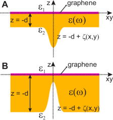
Figure 1: A dielectric protrusion (panel A) or indentation (panel B) below a flat graphene sheet. The defect is assumed to have either even parity symmetry (1D defect) or cylindrical symmetry (2D defect).

In all regions we write the electrostatic potential as a Fourier integral. In the first region we write

$$\phi_{1}(\boldsymbol{\rho},z,t)=\int\frac{d\mathbf{k}_{\parallel}}{(2\pi)^{2}}A(\mathbf{k}_{\parallel})\mathrm{e}^{\mathrm{i}\mathbf{k_{\parallel}}\cdot\boldsymbol{\rho}-k_{\parallel}z}\mathrm{e}^{-\mathrm{i}\omega t}\,,$$ (1)

where $\mathbf{k}_{\parallel}=(k_{x},k_{y})$ and $\boldsymbol{\rho}=(x,y)$. In the central region both real exponentials have to be present, that is,

$$\phi_{c}(\boldsymbol{\rho},z,t)=\int\frac{d\mathbf{k}_{\parallel}}{(2\pi)^{2}}[B(\mathbf{k}_{\parallel})\mathrm{e}^{k_{\parallel}z}+C(\mathbf{k}_{\parallel})\mathrm{e}^{-k_{\parallel}z}]\mathrm{e}^{\mathrm{i}\mathbf{k_{\parallel}}\cdot\boldsymbol{\rho}-\mathrm{i}\omega t}.$$ (2)

Finally, in the third region we have

$$\phi_{2}(\boldsymbol{\rho},z,t)=\int\frac{d\mathbf{k}_{\parallel}}{(2\pi)^{2}}D(\mathbf{k}_{\parallel})\mathrm{e}^{\mathrm{i}\mathbf{k_{\parallel}}\cdot\boldsymbol{\rho}+k_{\parallel}z}\mathrm{e}^{-\mathrm{i}\omega t}.$$ (3)

Next we assume that the above expressions for $\phi_{c}$ and $\phi_{2}$ hold in the region of bump/protrusion. The boundary conditions are imposed at $z=0$ and at $z=-d+\zeta(x,y)$, where $\zeta(x,y)$ is some even function, for example an inverted Gaussian:

$$\zeta(x,y)=-\zeta_{0}\mathrm{e}^{-\rho^{2}/s^{2}},$$ (4)

where $\rho^{2}=x^{2}+y^{2}$. At $z=0$ the boundary conditions are the same we have used for solving the flat graphene case discussed in Appendix A, whereas for $z=-d+\zeta(x,y)$, the boundary conditions are adapted from those at $z=0$ considering that $\sigma=0$ (the optical conductivity), and therefore the normal component of the electric displacement field is continuous through the interface. Although we have formulated the problem for a defect with cylindrical symmetry, we can also consider one-dimensional profiles, such as $\zeta(x)=-\zeta_{0}\mathrm{e}^{-4x^{2}/R^{2}}$, which will be the case considered next.

III A planar graphene sheet on a dielectric defect: 1D protrusion

From here on we consider a 1D defect. In this case the Fourier representation of the field is one-dimensional, reading

$$\phi_{1}(\boldsymbol{\rho},z,t)=\int\frac{dk_{x}}{2\pi}A(k_{x})\mathrm{e}^{\mathrm{i}(k_{x}x+k_{y}y)-k_{\parallel}z}e^{-\mathrm{i}\omega t},$$ (5)

and similar equations for $\phi_{c}$ and $\phi_{2}$. Next we want to obtain an eigenvalue equation, thus allowing us to determine the eigen-frequencies, in terms of a single coefficient. In particular, we want that coefficient to be $A(k_{x})$. For implementing the boundary conditions we need an expression for the normal derivative along the surface of the defect. This is given by

$$\frac{\partial}{\partial n}=\mathbf{\hat{n}}\cdot\nabla=\left[1+\left(\partial_{x}\zeta(x)\right)^{2}\right]^{-1/2}\left(-\partial_{x}\zeta(x)\partial_{x}+\partial_{z}\right).$$ (6)

At the interface $z=0$ we have simply

$$\frac{\partial}{\partial n}=\frac{\partial}{\partial z}.$$ (7)

Thus the boundary conditions are

$$\phi_{1}(\boldsymbol{\rho},0,t) =\phi_{c}(\boldsymbol{\rho},0,t),$$ (8a)

$$\epsilon_{1}\frac{\partial\phi_{1}(\boldsymbol{\rho},0,t)}{\partial z} -\epsilon(\omega)\frac{\partial\phi_{c}(\boldsymbol{\rho},0,t)}{\partial z}=-\frac{\mathrm{i}\sigma}{\epsilon_{0}\omega}\nabla_{2D}^{2}\phi(\boldsymbol{\rho},0,t),$$ (8b)

which turn into

$$A(k_{x}) =B(k_{x})+C(k_{x}),$$ (9a)

$$-\epsilon_{1}A(k_{x}) -\epsilon(\omega)[B(k_{x})-C(k_{x})]=\kappa A(k_{x}),$$ (9b)

where we defined:

$$\kappa\equiv\frac{\mathrm{i}\sigma k_{\parallel}}{\epsilon_{0}\omega},$$ (10)

and the solution for $B(k_{x})$ and $C(k_{x})$ reads

$$B(k_{x}) =A(k_{x})\frac{\epsilon(\omega)-\epsilon_{1}-\kappa}{2\epsilon(\omega)}\equiv A(k_{x})f_{+}(\omega,k_{\parallel}),$$ (11a)

$$C(k_{x}) =A(k_{x})\frac{\epsilon(\omega)+\epsilon_{1}+\kappa}{2\epsilon(\omega)}\equiv A(k_{x})f_{-}(\omega,k_{\parallel}).$$ (11b)

This allows us to write the field in the central region as a function of the $A(k_{x})$ alone. The next step is the implementation of the boundary conditions at the interface $z_{2c}(x)=-d+\zeta(x)$. These are

$$\phi_{c}(\boldsymbol{\rho},z_{2c}(x),t) =\phi_{2}(\boldsymbol{\rho},z_{2c}(x),t),$$ (12a)

$$\epsilon(\omega)\frac{\partial\phi_{c}(\boldsymbol{\rho},z_{2c}(x),t)}{\partial n} =\epsilon_{2}\frac{\partial\phi_{2}(\boldsymbol{\rho},z_{2c}(x),t)}{\partial n}.$$ (12b)

The boundary condition (12a) is simply given by

$$\int\frac{dk_{x}}{2\pi}A(k_{x})e^{\mathrm{i}(k_{x}x+k_{y}y)}\left[f_{+}(\omega,k_{\parallel})\mathrm{e}^{k_{\parallel}z_{2c}(x)}+\right.$$

$$\left.+f_{-}(\omega,k_{\parallel})\mathrm{e}^{-k_{\parallel}z_{2c}(x)}\right]=\int\frac{dk_{x}}{2\pi}D(k_{x})\mathrm{e}^{\mathrm{i}(k_{x}x+k_{y}y)}\mathrm{e}^{k_{\parallel}z_{2c}(x)}$$ (13)

The second boundary condition, Eq. (12b), reads

$$\epsilon_{2}\int\frac{dk_{x}}{2\pi}D(k_{x})\left[-\frac{\partial\zeta(x)}{\partial x}\mathrm{i}k_{x}+k_{\parallel}\right]\mathrm{e}^{\mathrm{i}(k_{x}x+k_{y}y)}\mathrm{e}^{k_{\parallel}z_{2c}(x)}=$$

$$\epsilon(\omega)\int\frac{dk_{x}}{2\pi}A(k_{x})\mathrm{e}^{\mathrm{i}(k_{x}x+k_{y}y)}\left[f_{+}(\omega,k_{\parallel})\mathrm{e}^{k_{\parallel}z_{2c}(x)}\times\right.$$

$$\times\left.\left(-\frac{\partial\zeta(x)}{\partial x}ik_{x}+k_{\parallel}\right)+f_{-}(\omega,k_{\parallel})\mathrm{e}^{-k_{\parallel}z_{2c}(x)}\times\right.$$

$$\left.\times\left(-\frac{\partial\zeta(x)}{\partial x}ik_{x}-k_{\parallel}\right)\right]$$ (14)

Now we need to combine Eqs. (13) and (14) for obtaining a single integral equation for the coefficient $A(k_{x})$. This is a more difficult task since we have the function $z_{2c}(x)$ in the exponent together with derivatives of $\zeta(x)$. For circumventing this difficulty we introduce the Fourier representation of the exponential $\mathrm{e}^{\alpha\zeta(x)}$ as

$$\mathrm{e}^{\alpha\zeta(x)}=1+\alpha\int\frac{dQ}{2\pi}J(\alpha;Q)e^{\mathrm{i}Qx},$$ (15)

where

$$J(\alpha;Q)=\int dx\mathrm{e}^{-\mathrm{i}Qx}\frac{\mathrm{e}^{\alpha\zeta(x)}-1}{\alpha}.$$ (16)

Equation (15) also implies that

$$\frac{\partial\zeta(x)}{\partial x}\mathrm{e}^{\alpha\zeta(x)}=\frac{1}{\alpha}\frac{\partial\mathrm{e}^{\alpha\zeta(x)}}{\partial x}=\int\frac{dQ}{2\pi}iQJ(\alpha;Q)\mathrm{e}^{\mathrm{i}Qx}.$$ (17)

Eqs. (15) and (17) allow the simplification of Eqs. (13) and (14). For eliminating the $D(k_{x})$ coefficient, we multiply Eq. (13) by

$$\left(\mathrm{i}q_{x}\frac{\partial\zeta(x)}{\partial x}+q_{\parallel}\right)e^{-\mathrm{i}(q_{x}x+q_{y}y)}\mathrm{e}^{q_{\parallel}\zeta(x)},$$ (18)

where $q_{\parallel}=q=\sqrt{q_{x}^{2}+q_{y}^{2}}$, and multiply Eq. (14) by $\mathrm{e}^{-\mathrm{i}(q_{x}x+q_{Y}y)}\mathrm{e}^{q_{\parallel}\zeta(x)}$. We then use Eqs. (15) and (17), and integrate over $\bm{\rho}=(x,y)$. After lengthy calculations we obtain a single equation involving the coefficient $A(k_{x})$ only:

$$\Gamma(q,\omega)A(q_{x})=\int_{-\infty}^{\infty}dP\,{\cal K}_{q_{y},\omega}(q_{x},P)A(P),$$ (19)

where $\hat{\mathbf{p}}=\mathbf{p}/p$, $\hat{\mathbf{q}}=\mathbf{q}/q$, $\mathbf{p}=(P,q_{y})$, $\mathbf{q}=(q_{x},q_{y})$, and

$$\Gamma(q,\omega)=[\epsilon_{2}-\epsilon(\omega)]^{-1}\left\{[\epsilon_{2}-\epsilon(\omega)]\mathrm{e}^{-qd}f_{+}(\omega,q)+\right.$$

$$\left.+[\epsilon_{2}+\epsilon(\omega)]\mathrm{e}^{qd}f_{-}(\omega,q)\right\},$$ (20)

with the Kernel:

$$\,{\cal K}_{q_{y},\omega}(q_{x},P)=pJ(q-p;q_{x}-P)f_{-}(\omega,p)\mathrm{e}^{pd}(1-$$

$$-\hat{\mathbf{p}}\cdot\hat{\mathbf{q}})-pJ(q+p;q_{x}-P)f_{+}(\omega,p)\mathrm{e}^{-pd}(1+\hat{\mathbf{p}}\cdot\hat{\mathbf{q}}).$$ (21)

IV Numerical solution

Eq. (19) is a homogeneous integral equation. In the following we discuss the classification of the integral equation as a Fredholm equation of second or third kind depending on the values of $q_{y}$ and $\omega$. If the equation:

$$\Gamma\left(\sqrt{q_{y}^{2}+q_{x}^{2}},\omega\right)=0,$$ (22)

has real solutions for a real $q_{x}$, the integral equation (19) is a Fredholm equation of the third kind. If not, is a Fredholm equation of the second kind. The curve $\Gamma\left(q_{y},\omega\right)=0$ separates the two regimes (see Fig. 2): the continuous solution and the localized plasmon states (see next Section for details). As we have $\hbar\omega\ll 2E_{F}$, the interband contributions are negligible. Thus we use the Drude formula for the optical conductivity of graphene without sacrificing accuracy.

From the curve $\Gamma\left(q_{y},\omega\right)=0$ we can test the validity of the electrostatic approximation. Noting that the decaying factor without the electrostatic approximation reads $\kappa_{i}=\sqrt{q_{y}^{2}+q_{x}^{2}-\varepsilon_{i}\omega^{2}/c^{2}}$, $i=1,2,3$, we have calculated for $q_{x}=0$, $q_{y}=0.4\,\mu$m^-1, and $E_{F}=0.3$ eV that the deviation $1-\kappa_{i}/q_{y}$ is no more than $4\%$ in the worst case scenario. Therefore, for the parameters used in the figures, the electrostatic approximation is justifiable.

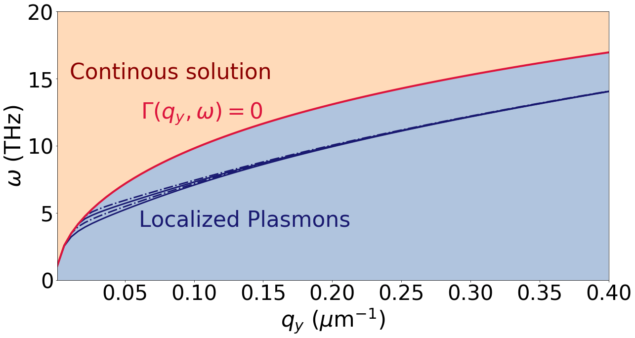
Figure 2: Transversely-localized plasmon dispersion. The solid red curve is the solution for $\Gamma(q_{y},\omega)=0$. For $\omega>\omega_{spp}$, the system admits continuous solutions, otherwise the solutions are transversely-localized plasmons. The parameters used are: $\varepsilon_{1}=1.4$, $\varepsilon_{2}=1$, $\varepsilon=4$, $E_{F}=0.2$ eV, $d=2\mu$m, $R=250\mu$m, and $\zeta_{0}=25\mu$m. The solid(dotted) blue curves are even(odd) solutions. We depict the first four transversely-localized plasmon modes for the parameters considered.

IV.1 Continuous solution

We first assume that Eq. (22) has solutions for real $q_{x}=\pm q_{x}^{0}$. In this condition Eq. (19) has not regular solutions, however considering a generalized functional space, the solution has the form Bart and Warnock (1973):

$$A(q_{x})=\alpha_{1}\delta(q_{x}-q_{x}^{0})+\alpha_{2}\delta(q_{x}+q_{x}^{0})+A_{\text{reg}}(q_{x}),$$ (23)

where $q_{x}^{0}$ is the solution of Eq. (22) and $A_{\text{reg}}(q_{x})$ is the regular part of the $A(q_{x})$. The coefficients $\alpha_{1}$ and $\alpha_{2}$ are determined putting Eq. (23) back to Eq. (19) and making $q_{x}=q_{x}^{0}$. We can separate the odd and even solutions by making $\alpha_{2}=\pm\alpha_{1}$. In the case that we set the protrusion to zero ($\zeta_{0}=0$), the regular part $A_{\text{reg}}(q_{x})=0$, and we simply recover the solution for the protrusion-free problem. Eq. (23) can be interpreted as the sum of the propagating waves from the protrusion-free problem $\alpha_{1}\delta(q_{x}-q_{x}^{0})+\alpha_{2}\delta(q_{x}+q_{x}^{0})$ plus a term that comes from the geometric effect of the protrusion.

The integral equation satisfied by the regular part of the solution is obtained substituting Eq. (23) back to Eq. (19):

$$\alpha_{1}{\cal K}_{q_{y},\omega}(q_{x},q^{0}_{x})+\alpha_{2}{\cal K}_{q_{y},\omega}(q_{x},-q^{0}_{x})+$$

$$+\int_{-\infty}^{\infty}dP\,{\cal K}_{q_{y},\omega}(q_{x},P)A_{\text{reg}}(P)=\Gamma(q,\omega)A_{\text{reg}}(q_{x}),$$ (24)

where we used the property obtained by the construction of the function (23):

$$\Gamma\left(\sqrt{q_{y}^{2}+q_{x}^{2}},\omega\right)A(q_{x})=\Gamma\left(\sqrt{q_{y}^{2}+q_{x}^{2}},\omega\right)A_{\text{reg}}(q_{x}).$$ (25)

Now, making $q_{x}=\pm q_{x}^{0}$, the coefficients $\alpha_{i}$ satisfy the system of equations:

$$\alpha_{1}{\cal K}_{q_{y},\omega}(q^{0}_{x},q^{0}_{x})+\alpha_{2}{\cal K}_{q_{y},\omega}(q^{0}_{x},-q^{0}_{x})+$$

$$+\int_{-\infty}^{\infty}dP\,{\cal K}_{q_{y},\omega}(q_{x}^{0},P)A_{\text{reg}}(P)=0,$$ (26a)

$$\alpha_{1}{\cal K}_{q_{y},\omega}(-q^{0}_{x},q^{0}_{x})+\alpha_{2}{\cal K}_{q_{y},\omega}(-q^{0}_{x},-q^{0}_{x})+$$

$$+\int_{-\infty}^{\infty}dP\,{\cal K}_{q_{y},\omega}(-q_{x}^{0},P)A_{\text{reg}}(P)=0,$$ (26b)

using the following kernel property ${\cal K}_{q_{y},\omega}(q_{x},P)={\cal K}_{q_{y},\omega}(-q_{x},-P)$ and that $A_{\text{reg}}(P)=\pm A_{\text{reg}}(-P)$ we obtain:

$$\int_{-\infty}^{\infty}dP\,\left[{\cal K}_{q_{y},\omega}(q_{x},P)-{\cal K}_{q_{y},\omega}(q^{0}_{x},P)\right]A_{\text{reg}}(P)=$$

$$=\Gamma(q,\omega)A_{\text{reg}}(q_{x}),$$ (27)

so, for a given $q_{y}$ and $\omega$, one has to solve (27) to obtain the field in the presence of the protrusion. Note that we have a continuous set of frequencies in this case.

IV.2 Transversely-localized plasmons

In the case where Eq. (22) has no real solutions for $q_{x}$, Eq. (19) is a homogeneous Fredholm equation of the second kind. This equation, for a given $q_{y}$, has solutions for some particular values of $\omega$. In the following, we consider the case where $\varepsilon(\omega)=\varepsilon$, that is, the dielectric function is independent of the frequency. In this case, Eq. (19) can be rewritten as:

$$\lambda(\omega){\cal D}_{1}(q_{x},q_{y})A={\cal D}_{2}(q_{x},q_{y})A,$$ (28)

where we have the following integral operators:

$${\cal D}_{1}(q_{x},q_{y})A=q^{2}\left[\frac{\varepsilon_{2}}{\varepsilon}\sinh(qd)+\cosh(qd)\right]A(q_{x})+$$

$$+\frac{\varepsilon_{2}-\varepsilon}{2\varepsilon}\int_{-\infty}^{\infty}\frac{dP}{2\pi}p\left[J(q+p,q_{x}-P)\mathrm{e}^{-pd}(q_{y}^{2}+pq+\right.$$

$$\left.+Pq_{x})+J(q-p,q_{x}-P)\mathrm{e}^{pd}(q_{y}^{2}-pq+Pq_{x})\right]A(P),$$ (29a)

$${\cal D}_{2}(q_{x},q_{y})A=\frac{q}{2\varepsilon}\left[(\varepsilon_{2}-\varepsilon)(\varepsilon-\varepsilon_{1})\mathrm{e}^{-qd}+(\varepsilon_{2}+\varepsilon)(\varepsilon+\right.$$

$$\left.+\varepsilon_{1})\mathrm{e}^{+qd}\right]A(q_{x})+\frac{\varepsilon_{2}-\varepsilon}{2\varepsilon}\int_{-\infty}^{\infty}\frac{dP}{2\pi}\left[(\varepsilon-\varepsilon_{1})\times\right.$$

$$\left.\times J(q+p,q_{x}-P)\mathrm{e}^{-pd}(q_{y}^{2}+pq+Pq_{x})+\right.$$

$$\left.+(\varepsilon+\varepsilon_{1})J(q-p,q_{x}-P)\mathrm{e}^{pd}(q_{y}^{2}-pq+Pq_{x})\right]A(P),$$ (29b)

and we defined:

$$\lambda(\omega)=-\mathrm{i}\frac{\sigma(\omega)}{\varepsilon_{0}\omega},$$ (30)

that has the dimension of length. To obtain those results we used:

$$f_{+}(\omega,p)=\frac{\varepsilon-\varepsilon_{1}}{2\varepsilon}+\frac{\lambda(\omega)p}{2\varepsilon},$$ (31a)

$$f_{-}(\omega,p)=\frac{\varepsilon+\varepsilon_{1}}{2\varepsilon}-\frac{\lambda(\omega)p}{2\varepsilon}.$$ (31b)

The integral operators ${\cal D}_{1}$ and ${\cal D}_{2}$ do not depend on the frequency $\omega$. To proceed, we discretize the integrals in Eqs. (29a) and (29b). First we apply a cutoff in the momentum $P$: $\int_{-\infty}^{\infty}\rightarrow\int_{-\Lambda}^{\Lambda}$, and $\Lambda$ is chosen to be large enough such that the solution converges (we checked that all boundary conditions are obeyed by the numerical solution). The integral can be discretized by applying Gauss-Legendre quadrature. This will reduce the integral [Eq. (28)] to a generalized eigenvalue problem:

$$\lambda(\omega)\mathbf{D}_{1}\mathbf{a}=\mathbf{D}_{2}\mathbf{a},$$ (32)

where $\mathbf{D}_{1/2}$ are $N\times N$ matrix, with $N$ the number of Gauss points, and $\mathbf{a}$ is a vector with dimension $N$ that represents the discretized version of the function $A(q_{x})$. Solving Eq. (32) we have the spectrum of eigenvalues $\lambda_{n}(q_{y})$. The plasmon frequency then is given by the solution of

$$\lambda(\omega)=\lambda_{n}(q_{y}).$$ (33)

If we assume that the conductivity of graphene is given by the Drude formula:

$$\sigma(\omega)=\sigma_{0}\frac{4i}{\pi}\frac{E_{F}}{\hbar\omega+i\hbar\gamma},$$ (34)

with $\sigma_{0}=e^{2}/(4\hbar)$, $E_{F}$ the Fermi energy, and $\gamma$ the relaxation rate, the plasmon dispersion is given by:

$$\omega_{n}(q_{y})=\sqrt{4c\alpha\frac{E_{F}}{\hbar}\frac{1}{\lambda_{n}(q_{y})}}-i\frac{\gamma}{2},$$ (35)

with $\alpha=1/137$ the fine structure constant and $c$ the speed of light. We can see from Eq. (35) that the transversely-localized plasmon linewidth is half that of the relaxation rate $\gamma$ in graphene. We have also compared the result obtained from (35) with a calculation that also included interband contributions to the optical conductivity and the difference for the frequency of the surface plasmons obtained as the solution of Eq. (33) is less than $1\%$.

Recalling the condition for the existence of transversely-localized plasmons, the solution of equation $\Gamma(q_{y},\omega)=0$ is:

$$\lambda(\omega)=\frac{b(q_{y})}{q_{y}},$$ (36)

with:

$$b(q_{y})=\frac{\varepsilon(\varepsilon_{2}+\varepsilon_{1})+(\varepsilon^{2}+\varepsilon_{1}\varepsilon_{2})\tanh(q_{y}d)}{\varepsilon+\varepsilon_{2}\tanh(q_{y}d)},$$ (37)

and using the definition of $\lambda(\omega)$, Eq. (30):

$$\omega_{\text{spp}}(q_{y})=\sqrt{4c\alpha\frac{E_{F}}{\hbar}\frac{q_{y}}{b(q_{y})}}-i\frac{\gamma}{2}.$$ (38)

Using the condition that, for the transversely-localized plasmons, $\lambda_{n}(q_{y})<\lambda(q_{y})$, we arrive at

$$\lambda_{n}(q_{y})q_{y}>b(q_{y}).$$ (39)

The latter relation defines the region of existence of SPP and does not depend on properties of the graphene sheet, that is, it is a purely geometric condition.

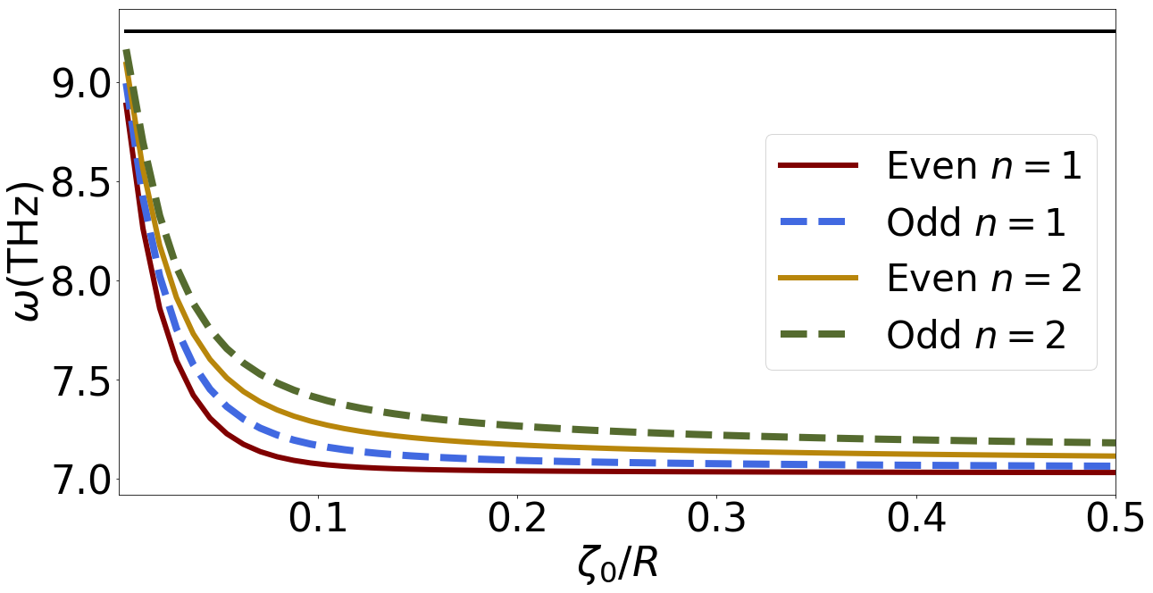
Figure 3: Dependence on the ratio $\zeta_{0}/R$. The black line at $\approx 11$ THz is the solution for $\Gamma(q_{y},\omega)=0$, i.e., the maximum frequency for transversely-localized plasmons. Parameters: $\varepsilon_{1}=1.4$, $\varepsilon_{2}=1$, $\varepsilon=4$, $E_{F}=0.2$ eV, $d=2\mu$m, $R=250\mu$m, $q_{y}=0.1\mu\mathrm{m}^{-1}$. We clearly see that for $\zeta_{0}/R\approx 0.2$ the frequency of the transversely-localized plasmon reaches a plateau.

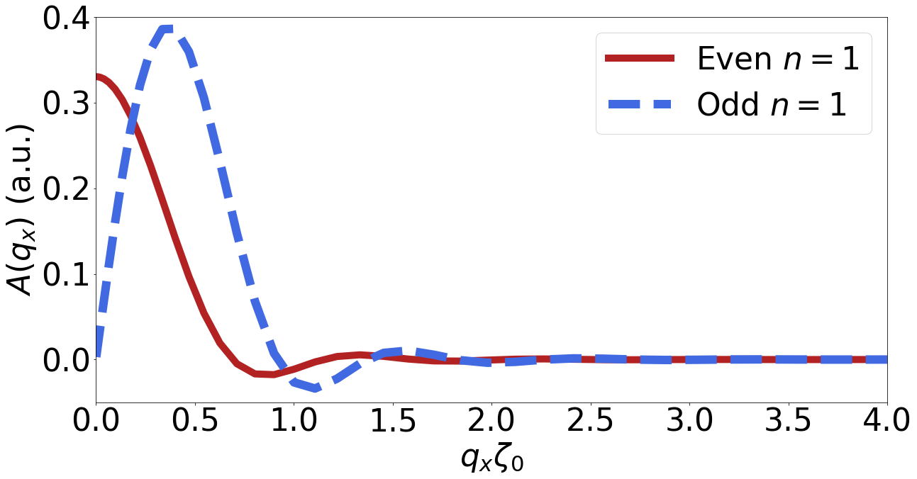
Figure 4: Solutions for the generalized eigenvalue problem. The solid red (dashed blue) curve is the first even (odd) solution. Parameters: $\varepsilon_{1}=1.4$, $\varepsilon_{2}=1$, $\varepsilon=4$, $E_{F}=0.2$ eV, $d=2\mu$m, $R=250\mu$m, $\zeta_{0}=25\mu$ m, $q_{y}=0.4\mu\text{m}^{-1}$.

Once we compute the coefficient $A(q_{x})$, the coefficients $B(q_{x})$ and $C(q_{x})$ are calculated using Eqs. (11a) and (11b):

$$B(k_{x}) =A(k_{x})\frac{\epsilon(\omega)-\epsilon_{1}-\kappa}{2\epsilon(\omega)},$$ (40a)

$$C(k_{x}) =A(k_{x})\frac{\epsilon(\omega)+\epsilon_{1}+\kappa}{2\epsilon(\omega)}.$$ (40b)

The equation for $D(q_{x})$ can be obtained from the boundary condition (13), using the same procedure that was used to obtain the Eq. (19):

$$qe^{-qd}D(q_{x})+\int_{-\infty}^{\infty}\frac{dP}{2\pi}J(q+p,q_{x}-P)\mathrm{e}^{-pd}(q_{y}^{2}+pq+q_{x}P)D(P)=q\left(\frac{\varepsilon-\varepsilon_{1}}{2\varepsilon}\mathrm{e}^{-qd}+\frac{\varepsilon+\varepsilon_{1}}{2\varepsilon}\mathrm{e}^{qd}-\right.$$

$$\left.-q\lambda(\omega)\frac{\sinh(qd)}{\varepsilon}\right)A(q_{x})+\int_{-\infty}^{\infty}\frac{dP}{2\pi}\left[(q_{y}^{2}+pq+Pq_{x})f_{+}(\omega,p)J(q+p,q_{x}-P)\mathrm{e}^{-pd}+\right.$$

$$\left.+(q_{y}^{2}-pq+Pq_{x})f_{-}(\omega,p)J(q-p,q_{x}-P)\mathrm{e}^{pd}\right]A(P),$$ (41)

which can be written in a matrix from as:

$$\mathbf{G}_{1}\mathbf{d}=\mathbf{G}_{2}\mathbf{a},$$ (42)

where $\mathbf{G}_{1}$ and $\mathbf{G}_{2}$ are the discrete versions of the operators appearing in Eq. (41) and $\mathbf{d}$ is the corresponding discretized $D(q_{x})$ vector. From the previous equation, have the elementary solution:

$$\mathbf{d}=\mathbf{G}_{1}^{-1}\mathbf{G}_{2}\mathbf{a},$$ (43)

which, since $\mathbf{a}$ has been previously obtained, readily gives the values for $\mathbf{d}$ by matrix multiplication.

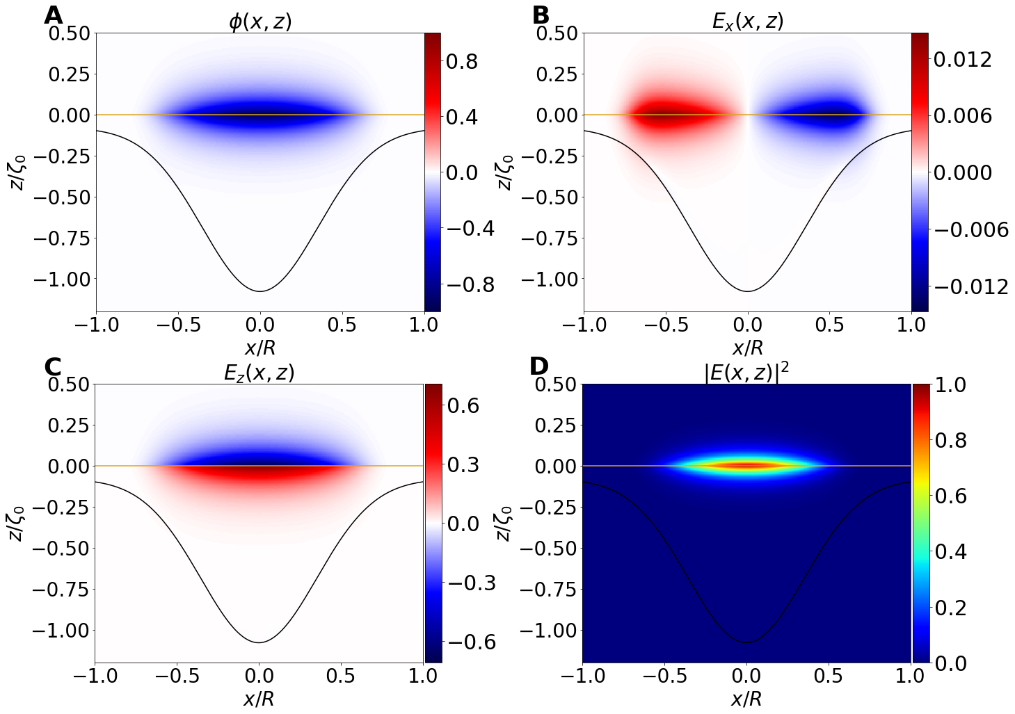
Figure 5: Transversely-localized plasmon potential and electric fields for the system illustrated in Fig 1(a). The black line shows the boundary between the regions of dielectric $\varepsilon$ and $\varepsilon_{2}$ and the gold line represents the graphene sheet. The color represents the intensity of the field in arbitrary units. The electric fields in panels B, C and D are normalized by the maximum value of the total electric field. For the panels B and C the red and blue colors define a change of phase of $\pi$. We show the results for the first even solution. Panels A) Potential Field, B) $x-$ component of the Electric Field, C) $z-$ component of the electric field, D) Square of the absolute value of the electric field. Parameters: $\varepsilon_{1}=1.4$, $\varepsilon_{2}=1$, $d=2\mu$m, $R=250\mu$m, $\zeta_{0}=25\mu$ m, $q_{y}=0.4\mu\text{m}^{-1}$. Note that those fields do not depend on the properties of the graphene sheet.

V Results

From here on, we consider that the protrusion/indentation is described by a Gaussian profile:

$$\zeta(x)=-\zeta_{0}e^{-4x^{2}/R^{2}},$$ (44)

with the sign of $\zeta_{0}$ defining the two different cases schematically illustrated in Figs. 1(A) and 1(B). In Appendix B we calculate the $J(\alpha;Q)$ function [Eq. (16)] for the Gaussian profile.

From here on, we will consider the transversely-localized plasmons case only, that is, for a given $q_{y}$, the maximum frequency that we consider is given by Eq. (38). Otherwise specified, we use the following parameters: $\varepsilon_{1}=1.4$, $\varepsilon_{2}=1$, $\varepsilon=4$, $E_{F}=0.2$ eV, $\gamma=0$, $d=2\,\mu$m, $R=250\,\mu$m, and $\zeta_{0}=25\,\mu$m. The numerical parameters are $N=100$ Gauss numbers and the cutoff $\Lambda=12/\zeta_{0}$. These parameters illustrate the implications of the method, but choosing other values amounts to quantitative changes only.

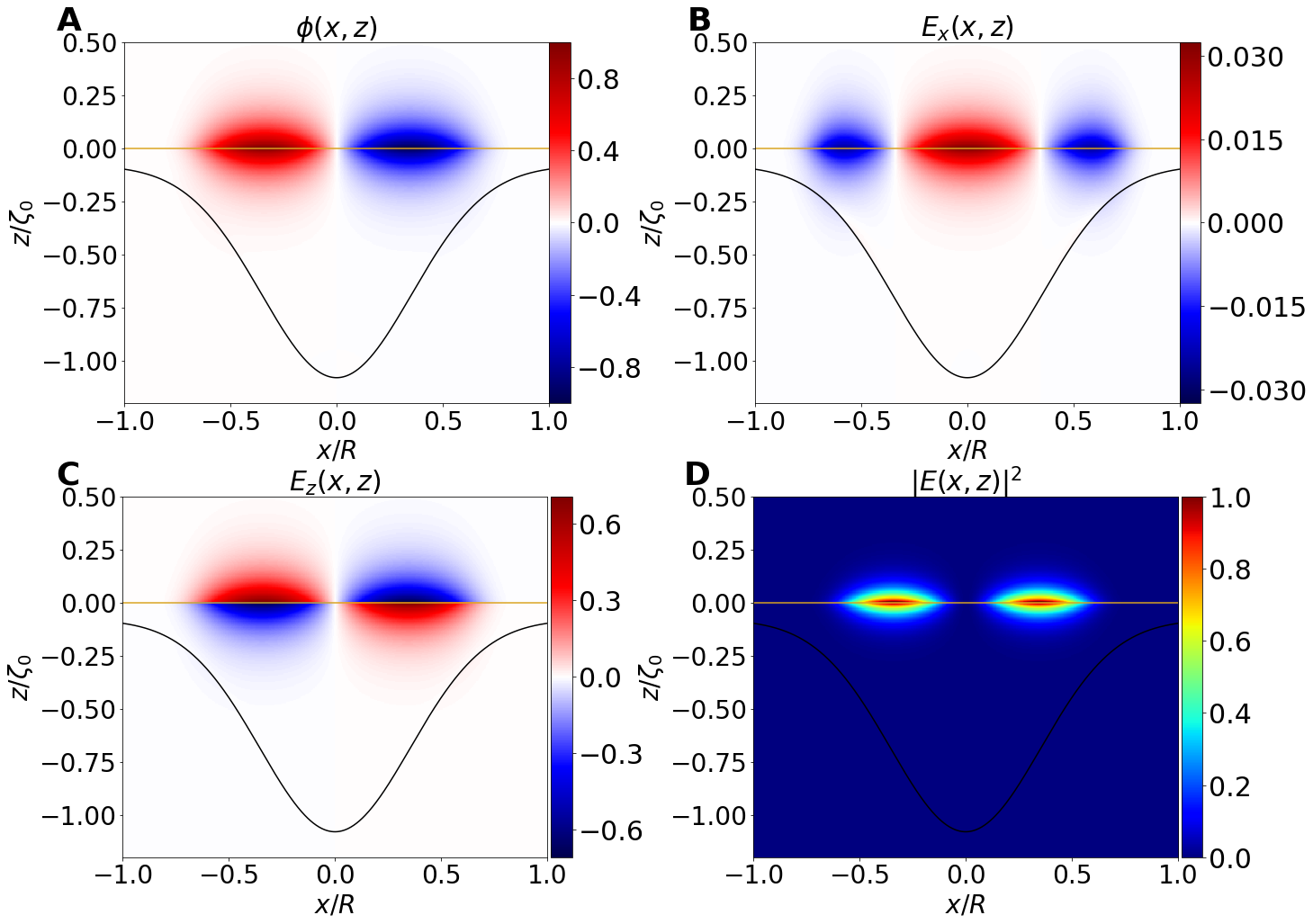
Figure 6: The same as Fig. 5, but now for the first odd solution.

V.1 Parity

The Kernel of the integral Eq. (19) obeys the identity:

$${\cal K}(q_{x},P)={\cal K}(-q_{x},-P),$$ (45)

and the function $\Gamma(q_{x},\omega)$ is even in the $q_{x}$ variable. From this condition the solutions can be classified in odd and even. Therefore, the limits of integration can be changed as: $\int_{-\Lambda}^{\Lambda}\rightarrow\int_{0}^{\Lambda}$, which simplifies the numerical solution.

V.2 Scale invariance

Here we consider how the spectrum changes upon a scale transformation. Making the scale transformation: $d\rightarrow\xi d$, $R\rightarrow\xi R$, $\zeta_{0}\rightarrow\xi\zeta_{0}$ and $q_{y}\rightarrow q_{y}/\xi$ makes the Kernels of Eq. (28) transform Eq. (29a) to ${\cal D}_{1}(q_{x},q_{y})\rightarrow\xi^{-2}{\cal D}_{1}(q_{x}/\xi,q_{y}/\xi)$ and Eq. (29b) ${\cal D}_{2}(q_{x},q_{y})\rightarrow\xi^{-1}{\cal D}_{2}(q_{x}/\xi,q_{y}/\xi)$ . Therefore the eigenvalue $\lambda_{n}$ of the matrix equation (28) transform to $\lambda_{n}\rightarrow\xi\lambda_{n}$. From Eq. (35) the frequency of the transversely-localized plasmon scale as $\omega_{n}(q_{y})\rightarrow\xi^{-1}\omega_{n}(q_{y}/\xi)$. This simple transformation of the eigen-frequencies upon a scale transformation is due to the electrostatic limit we have considered from the outset.

From this discussion, only the ratios $\zeta_{0}/R$ and $d/R$ matters for the calculation of the dispersion relation. In Fig. 3 we show the dependence on the plasmon frequency for fixed $R$ and $d$ as function of $\zeta_{0}$, where we can see clearly two regimes: for $\zeta_{0}/R<0.2$, we have a fast change in the localization frequency starting from the continuous solution (maximum localized frequency), and for $\zeta_{0}/R>0.2$ the system reaches a plateau and the change in the plasmon frequency is negligible.

V.3 Discussion

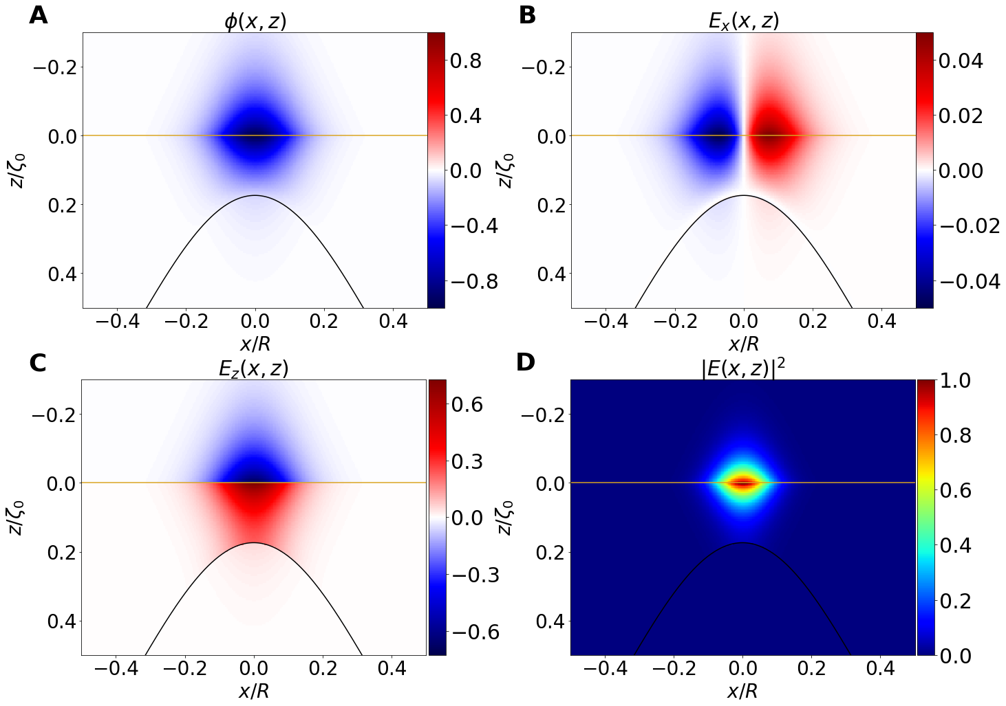
Figure 7: Transversely-localized plasmon potential and electric fields for the system illustrated in Fig 1(b). The black line shows the boundary between the regions of dielectric $\varepsilon$ and $\varepsilon_{2}$ and the gold line represents the graphene sheet. The color represents the intensity of the field in arbitrary units. The electric fields in panels B, C and D are normalized by the maximum value of the total electric field. For the panels B and C the red and blue colors define a change of phase of $\pi$. We show the results for the first even solution. Panels A) Potential Field, B) $x-$ component of the Electric Field, C) $z-$ component of the electric field, D) Square of the absolute value of the electric field. Parameters: $\varepsilon_{1}=1$, $\varepsilon_{2}=6$, $\varepsilon=1.4$, $d=27\mu$m, $R=250\mu$m, $\zeta_{0}=-23\mu$ m, $q_{y}=0.4\mu\text{m}^{-1}$.

Figure 8: The same as Fig. 7, but now for the first odd solution.

First we show in Fig. 4 the solution for the generalized eigenvalue problem (28) for the first even and odd solutions and $q_{y}=0.4\mu\text{m}^{-1}$, where we can see that the functions $A(q_{x})$ approach zero for $q_{x}\zeta_{0}\approx 2$.

Using Eqs. (11a), (11b), and (41) we can compute all the other functions $B(q_{x})$, $C(q_{x})$, and $D(q_{x})$. The potential field can be calculated now from [see Eqs. (1), (2),and (3)]:

$$\phi_{1}(x,0,z,0) =\int_{-\infty}^{\infty}\frac{dP}{2\pi}A(P)\mathrm{e}^{\mathrm{i}Px}\mathrm{e}^{-pz},$$ (46a)

$$\phi_{\text{c}}(x,0,z,0) =\int_{-\infty}^{\infty}\frac{dP}{2\pi}\mathrm{e}^{\mathrm{i}Px}\left(B(P)\mathrm{e}^{-pz}+C(P)\mathrm{e}^{pz}\right),$$ (46b)

$$\phi_{2}(x,0,z,0) =\int_{-\infty}^{\infty}\frac{dP}{2\pi}D(P)\mathrm{e}^{\mathrm{i}Px}\mathrm{e}^{pz},$$ (46c)

where for simplicity we are only interested for the results to $y=0$ and $t=0$, because of time and $y-$ translation invariance. The electric field can be obtained from $\mathbf{E}=-\boldsymbol{\nabla}\phi$, with $E_{y,i}=-\mathrm{i}k_{y}\phi_{i}$, where $i=1,2,\text{c}$ labeling the three regions. The other two components are:

$$E_{x,1}(x,y=0,z,t=0) =-\mathrm{i}\int_{-\infty}^{\infty}\frac{dP}{2\pi}PA(P)\mathrm{e}^{\mathrm{i}Px}\mathrm{e}^{-pz},$$ (47a)

$$E_{z,1}(x,y=0,z,t=0) =\int_{-\infty}^{\infty}\frac{dP}{2\pi}pA(P)\mathrm{e}^{\mathrm{i}Px}\mathrm{e}^{-pz},$$ (47b)

and similar expressions for the regions $2$ and c. First we note that from the parity symmetry of the system, the normalization of the field $A(P)$ can be choose such that $\phi_{i}$ will be always a real quantity. With a real $\phi_{i}$, the electric fields $E_{x,i}$ and $E_{z,i}$ will also be real and $E_{y,i}$ will be a pure imaginary quantity, i.e., it will always be out-of-phase by $\pi/2$ with the other electric field components.

From Eqs. (46a)–(47b) we calculate the potential and electrical field in Fig. 5, for the first even solution and in Fig. 6 for the first odd solution in a Gaussian 1D protrusion. For those solutions the plasmon frequencies are $\omega_{\text{even}}=14.04$ THz and $\omega_{\text{odd}}=14.05$ THz, respectively. The even solution has a node at $x=0$, as it should be, and the field strength, as can be seen in the panel D, is concentrated in the $x$ axis for $x\approx 0.25R=60\mu m$ and in the $y$ axis around $y\approx 0.1\zeta_{0}\approx 2.5\mu m$, far below the wavenumber $\lambda=134\mu$m for the light in air. We have verified that the fields obtained by Eqs. (46a)–(47b) satisfy all the boundary conditions. In Figs. 7 and 8 we show the transversely-localized plasmons in a groove (Gaussian indentation), where we can see that the field is less localized in the $y$ axis in comparison with the protrusion case. However, the indentation “squeezes" the plasmon in the central region. A remarkable characteristic of the electrostatic approximation is that all the fields profile are only a geometric solution of the integral equation, that is, they do not depend on the properties of the graphene sheet. However, they can only exist if Eq. (33) has solution. Therefore, without the graphene sheet there are no transversely-localized plasmons.

We also note that the Fermi-energy $E_{F}$ can be used to tune the frequency of the transversely-localized plasmons as per Eq. (35). Another important result of our study is that the transversely-localized plasmon dispersion is always below the usual SPP dispersion (see Fig. 2). Therefore, for a given frequency, the wavelength of the transversely-localized plasmons is always smaller than its value for a continuous graphene sheet on a homogeneous dielectric, implying a higher degree of confinement of the plasmons in dielectric with a protrusion/indentation.

The charge density can be calculated using the equivalent of Eq. (52):

$$n_{\text{2D}}(x)=-\lambda(\omega)\int_{-\infty}^{\infty}\frac{dP}{2\pi}(P^{2}+k_{y}^{2})A(P)\mathrm{e}^{\mathrm{i}Px},$$ (48)

and we show the charge density for the first two modes in the groove in Fig. 9, where we can see again that the charge is localized around $x\approx 0.5R$ the center of the wedge. Finally, we note that we have used a Gaussian profile but our approach can be used to any differentiable profile.

Figure 9: Charge density at the graphene sheet. Solid red (dashed blue) curve is the first even (odd) solution. Parameters: $\varepsilon_{1}=1.4$, $\varepsilon_{2}=1$, $\varepsilon=4$, $E_{F}=0.2$ eV, $d=2\mu$m, $R=250\mu$m, $\zeta_{0}=25\mu$ m, $q_{y}=0.4\mu\text{m}^{-1}$.

VI Conclusions

In this paper we have developed an approach of creating transversely localized plasmons in a flat graphene sheet. This is possible in a configuration where graphene rests on a flat substrate with the opposite surface of the latter showing a protrusion or and indentation (a defect). The transversely-localized plasmons dispersion relation appears below the dispersion relation of the propagating plasmons when graphene rests on a flat dielectric of thickness $d$. Above this latter dispersion relation, we have found a continuum of states, which would be needed for describing scattering by the defect. Therefore, we have shown that a defect (in this case with even symmetry) can trap localized surface plasmons. Since the defect is 1D, the wave number along the axis of symmetry of the defect is well defined and, therefore, this defect can also act as channel for propagation of the transversely-localized surface plasmons. This geometry has the advantage of being unnecessary to pattern the graphene sheet, therefore it works without deteriorating the electronic mobility of graphene. The generalization of the problem dealt in this paper to a 2D defect is straightforward, involving only extra computer power. This is no impediment as our codes are fast enough and run in a laptop in only few minutes.

Appendix A A planar graphene sheet

Let us assume a graphene sheet located at $z=0$ in the $xy-$plane. The graphene is capped by two dielectrics with dielectric functions $\epsilon_{1}$, for $z>0$, and $\epsilon_{2}$, for $z<0$. We want to find the spectrum of graphene SPP. The solution of Laplace’s equation for $z>0$ reads

$$\phi_{1}(\mathbf{\bm{\rho}},z,t)=A_{1}e^{i\mathbf{k}_{\parallel}\cdot\mathbf{\bm{\rho}}}e^{-k_{\parallel}z}e^{-i\omega t}\equiv\phi_{1}(\bm{\rho},z,\omega)e^{-i\omega t},$$ (49)

where $\mathbf{k}_{\parallel}=(k_{x},k_{y})$ and $\bm{\rho}=(x,y)$, and for $z<0$ it is given by

$$\phi_{2}(\mathbf{\bm{\rho}},z,t)=A_{2}e^{i\mathbf{k}_{\parallel}\cdot\mathbf{\bm{\rho}}}e^{k_{\parallel}z}e^{-i\omega t}\equiv\phi_{2}(\bm{\rho},z,\omega)e^{-i\omega t}.$$ (50)

The boundary conditions are

$$\phi_{1}(\bm{\rho},0,t) =\phi_{2}(\bm{\rho},0,t)$$ (51a)

$$\epsilon_{1}\frac{\partial\phi_{1}(\bm{\rho},0,t)}{\partial n} -\epsilon_{2}\frac{\partial\phi_{2}(\bm{\rho},0,t)}{\partial n}=-\frac{n_{2D}(\bm{\rho},0,t)}{\epsilon_{0}},$$ (51b)

where $n_{2D}(\bm{\rho},0,t)$ is the charge density in graphene, whose time dependence can be explicitly made as $n_{2D}(\bm{\rho},0,t)=n_{2D}(\bm{\rho},0,\omega)e^{-i\omega t}$. The first boundary condition expresses the continuity of the electrostatic potential and the second one the discontinuity of the normal component of the displacement vector. In addition, the electronic density obeys the continuity equation in frequency space: $i\omega n_{2D}(\bm{\rho},0,\omega)=\nabla_{2D}\cdot\mathbf{J}_{2D}(\bm{\rho},0,\omega)$, where $\nabla_{2D}=(\partial/\partial_{x},\partial/\partial_{y})$. Since the electric current density obeys Ohm’s law, $\mathbf{J}_{2D}(\bm{\rho},0,\omega)=-\sigma\nabla_{2D}\phi(\bm{\rho},0,\omega)$, it follows that

$$i\omega n_{2D}(\bm{\rho},0,\omega) =-\sigma\nabla_{2D}^{2}\phi(\bm{\rho},0,\omega)=\sigma k_{\parallel}^{2}\phi(\bm{\rho},0,\omega).$$ (52)

Finally, we have for the 2D electronic density the result

$$n_{2D}(\bm{\rho},0,\omega)=-\frac{i\sigma}{\omega}k_{\parallel}^{2}\phi(\bm{\rho},0,\omega)$$ (53)

The first boundary condition implies $A_{1}=A_{2}$ and the second boundary condition gives

$$-\epsilon_{1}k_{\parallel}-\epsilon_{2}k_{\parallel}=\frac{i\sigma}{\omega\epsilon_{0}}k_{\parallel}^{2}$$ (54)

or

$$\frac{\epsilon_{1}}{k_{\parallel}}+\frac{\epsilon_{2}}{k_{\parallel}}+\frac{i\sigma}{\omega\epsilon_{0}}=0,$$ (55)

which is the condition giving the dispersion relation of the SPP in graphene, Note that for $\sigma=0$ we recover the condition giving the dispersion of SPP at the interface between two dielectrics. In general, we should have written the electrostatic potential as

$$\phi_{1}(\boldsymbol{\rho},z,t) =\int\frac{d\mathbf{k}_{\parallel}}{(2\pi)^{2}}A_{1}(\mathbf{k}_{\parallel})e^{i\mathbf{k}_{\parallel}\cdot\mathbf{\boldsymbol{\rho}}}e^{-k_{\parallel}z}e^{-i\omega t},$$ (56)

and an identical expression for $\phi_{2}(\bm{\rho},t)$, except for the dependence $e^{-k_{\parallel}z}$ which should by replaced by $e^{k_{\parallel}z}$. This way of writing the electrostatic potential is appropriate for discussing rough surface and defects.

Appendix B The case of a Gaussian profile

In this appendix we give the evaluation of the function $J(\alpha;Q)$ for the Gaussian profile. This is accomplished by expanding the exponential of $\zeta(x)$ in the integrand, that is,

$$J(\alpha;Q) =\int_{-\infty}^{\infty}dx\mathrm{e}^{-\mathrm{i}Qx}\frac{\mathrm{e}^{\alpha\zeta(x)}-1}{\alpha}=$$

$$=\sum_{n=1}^{\infty}\int_{-\infty}^{\infty}dx\mathrm{e}^{-\mathrm{i}Qx}\frac{\alpha^{n-1}}{n!}\zeta^{n}(x).$$ (57)

Therefore we need to compute the integral (the Fourier transform of a Gaussian)

$$I(n;Q) =(-\zeta_{0})^{n}\int_{-\infty}^{\infty}dx\mathrm{e}^{-\mathrm{i}Qx}\mathrm{e}^{-4nx^{2}/R^{2}}$$

$$=(-\zeta_{0})^{n}\frac{R\sqrt{\pi}}{2\sqrt{n}}\mathrm{e}^{-Q^{2}R^{2}/(16n)}.$$ (58)

We have then

$$J(\alpha;Q)=\frac{R^{2}\sqrt{\pi}}{2}\sum_{n=1}^{\infty}\frac{(\alpha R)^{n-1}}{\sqrt{n}n!}(-\zeta_{0}/R)^{n}\mathrm{e}^{-Q^{2}R^{2}/(16n)},$$ (59)

which is a purely geometric quantity.

References

- Ju et al. (2011) L. Ju, B. Geng, J. Horng, C. Girit, M. Martin, Z. Hao, H. A. Bechtel, X. Liang, A. Zettl, Y. R. Shen, et al., Nat. Nanotechnol. 6, 630 (2011).
- Yan et al. (2012) H. Yan, X. Li, B. Chandra, G. Tulevski, Y. Wu, M. Freitag, W. Zhu, P. Avouris, and F. Xia, Nat. Nanotechnol. 7, 330 (2012).
- Gonçalves and Peres (2016) P. A. D. Gonçalves and N. M. R. Peres, An Introduction to Graphene Plasmonics (World Scientific, Singapore, 2016).
- Basov et al. (2016) D. Basov, M. Fogler, and F. G. de Abajo, Science 354, aag1992 (2016).
- Low et al. (2017) T. Low, A. Chaves, J. D. Caldwell, A. Kumar, N. X. Fang, P. Avouris, T. F. Heinz, F. Guinea, L. Martin-Moreno, and F. Koppens, Nature materials 16, 182 (2017).
- Atwater (2007) H. A. Atwater, Scientific American 296, 56 (2007).
- Brolo (2012) A. G. Brolo, Nature Photonics 6, 709 (2012).
- Acimovic et al. (2014) S. S. Acimovic, M. A. Ortega, V. Sanz, J. Berthelot, J. L. Garcia-Cordero, J. Renger, S. J. Maerkl, M. P. Kreuzer, and R. Quidant, Nano letters 14, 2636 (2014).
- Rodrigo et al. (2015) D. Rodrigo, O. Limaj, D. Janner, D. Etezadi, F. J. G. de Abajo, V. Pruneri, and H. Altug, Science 349, 165 (2015).
- Green and Pillai (2012) M. A. Green and S. Pillai, Nat. Photonics 6, 130 (2012).
- Reece (2008) P. J. Reece, Nature Photonics 2, 333 (2008).
- Juan et al. (2011) M. L. Juan, M. Righini, and R. Quidant, Nat. Photonics 5, 349 (2011).
- Huidobro et al. (2010) P. A. Huidobro, M. L. Nesterov, L. Martín-Moreno, and F. J. García-Vidal, NanoLetters 10, 1985 (2010).
- Pendry et al. (2012) J. Pendry, A. Aubry, D. Smith, and S. Maier, Science 337, 549 (2012).
- Smith et al. (2015) C. L. C. Smith, N. Stenger, A. Kristensen, N. A. Mortensen, and S. I. Bozhevolnyi, Nanoscale 7, 9355 (2015).
- Nielsen et al. (2008) R. B. Nielsen, I. Fernandez-Cuesta, A. Boltasseva, V. S. Volkov, S. I. Bozhevolnyi, A. Klukowska, and A. Kristensen, Opt. Lett. 33, 2800 (2008).
- Gramotnev and Pile (2004) D. K. Gramotnev and D. F. P. Pile, Appl. Phys. Lett. 85, 6323 (2004).
- Jablan et al. (2009) M. Jablan, H. Buljan, and M. Soljačić, Physical review B 80, 245435 (2009).
- Tassin et al. (2012) P. Tassin, T. Koschny, M. Kafesaki, and C. M. Soukoulis, Nature Photonics 6, 259 (2012).
- Wenger et al. (2016) T. Wenger, G. Viola, M. Fogelström, P. Tassin, and J. Kinaret, Physical Review B 94, 205419 (2016).
- Xiao et al. (2016) S. Xiao, X. Zhu, B.-H. Li, and N. A. Mortensen, Front. Phys. 11, 117801 (2016).
- García de Abajo (2014) F. J. García de Abajo, ACS Photonics 1, 135 (2014).
- Gonçalves et al. (2017a) P. A. D. Gonçalves, S. Xiao, N. Peres, and N. A. Mortensen, ACS Photonics (2017a).
- Liu et al. (2013) P. Liu, X. Zhang, Z. Ma, W. Cai, L. Wang, and J. Xu, Opt. Express 21, 32432 (2013).
- Smirnova et al. (2016) D. Smirnova, S. H. Mousavi, Z. Wang, Y. S. Kivshar, and A. B. Khanikaev, ACS Photonics 3, 875 (2016).
- Gonçalves et al. (2017b) P. A. D. Gonçalves, S. I. Bozhevolnyi, N. A. Mortensen, and N. Peres, Optica 4, 595 (2017b).
- Maradudin and Visscher (1985) A. Maradudin and W. Visscher, Z. Phys. B Cond. Matter 60, 215 (1985).
- Sturman et al. (2014) B. Sturman, E. Podivilov, and M. Gorkunov, JOSA B 31, 1607 (2014).
- Mayergoyz et al. (2005) I. D. Mayergoyz, D. R. Fredkin, and Z. Zhang, Phys. Rev. B 72, 155412 (2005).
- Arias and Maradudin (2013) R. E. Arias and A. A. Maradudin, Optics express 21, 9734 (2013).
- Zayats et al. (2005) A. V. Zayats, I. I. Smolyaninov, and A. A. Maradudin, Phys. Rep. 408, 131 (2005).
- Raether (1988) H. Raether, in Surface plasmons on smooth and rough surfaces and on gratings (Springer, 1988) pp. 4–39.
- Pereira et al. (2003) J. M. Pereira, G. Farias, and R. Costa Filho, Eur. Phys. J. B. 36, 137 (2003).
- Chubchev et al. (2017) E. Chubchev, I. Nechepurenko, A. Dorofeenko, A. Vinogradov, and A. Lisyansky, arXiv preprint arXiv:1711.08115 (2017).
- García de Abajo (2013) F. J. García de Abajo, ACS nano 7, 11409 (2013).
- Kumar et al. (2015) A. Kumar, T. Low, K. H. Fung, P. Avouris, and N. X. Fang, Nano letters 15, 3172 (2015).
- Bart and Warnock (1973) G. Bart and R. Warnock, SIAM J. on Math. Anal. 4, 609 (1973).