A method for determining the radius of an open cluster from stellar proper motions

Abstract

We propose a method for calculating the radius of an open cluster in an objective way from an astrometric catalogue containing, at least, positions and proper motions. It uses the minimum spanning tree (hereinafter MST) in the proper motion space to discriminate cluster stars from field stars and it quantifies the strength of the cluster-field separation by means of a statistical parameter defined for the first time in this paper. This is done for a range of different sampling radii from where the cluster radius is obtained as the size at which the best cluster-field separation is achieved. The novelty of this strategy is that the cluster radius is obtained independently of how its stars are spatially distributed. We test the reliability and robustness of the method with both simulated and real data from a well-studied open cluster (NGC 188), and apply it to UCAC4 data for five other open clusters with different catalogued radius values. NGC 188, NGC 1647, NGC 6603 and Ruprecht 155 yielded unambiguous radius values of $15.2\pm 1.8$, $29.4\pm 3.4$, $4.2\pm 1.7$ and $7.0\pm 0.3$ arcmin, respectively. ASCC 19 and Collinder 471 showed more than one possible solution but it is not possible to know whether this is due to the involved uncertainties or to the presence of complex patterns in their proper motion distributions, something that could be inherent to the physical object or due to the way in which the catalogue was sampled.

1 Introduction

Star clusters have long been recognized as very useful tools in many areas of astronomy including, among others, the structure and evolution of the Milky Way (see for instance Gilmore et al., 2012; Randich et al., 2013; Moraux, 2016). A precise knowledge of cluster properties such as distance, age, metallicity or reddening is necessary in order to be able to draw reliable conclusions. Large open cluster catalogues, like that published by Dias et al. (2002, 2014), compile all the available information required to make studies on, for instance, the rotation of the spiral patterns (Dias & Lépine, 2005) or the Galactic star formation history (de la Fuente Marcos & de la Fuente Marcos, 2004). However, this kind of data collections has the disadvantage of being highly heterogeneous. With the increasing number of publicly available photometric and astrometric databases, there is a growing interest in the automated and systematic estimation of homogeneous parameters for Galactic cluster (e.g. Kharchenko et al., 2012; Dias et al., 2014; Krone-Martins & Moitinho, 2014; Sarro et al., 2014; Perren et al., 2015; Sampedro et al., 2017). The catalogue by Kharchenko et al. (2013), mainly based on the PPMXL catalogue (Roeser et al., 2010), provides basic astrophysical data for a large set of clusters derived in a uniform and homogeneous way. There is however a need for some caution in this kind of massive data processing because slight variations in the developed strategies can lead to significant biases in the inferred cluster parameters. Netopil et al. (2015) compared the parameters given in several catalogues (including Kharchenko et al., 2013) and concluded that there are clear discrepancies and trends in distances, reddenings and ages.

Cluster radius is a particularly valuable parameter because it is a common strategy to choose the size of the field of view surrounding the cluster very close to cluster size in order to minimize contamination by field stars. In fact, Sanchez et al. (2010) have shown that, when estimating cluster memberships for a mixture of two Gaussian distributions, a sampling radius larger than the cluster radius may produce a severe contamination by field stars in the identified cluster members (spurious members) that certainly affects the determination of the remaining cluster properties. Apart from visual inspection, the standard method for directly estimating cluster radii is based on their projected radial density profiles. Usually, a King-like function (or any other analytical function) is fitted to the density profile and the cluster radius is extracted from this fit. Systematic determinations of cluster sizes based on this strategy have been performed by Kharchenko et al. (2005a, 2012, 2013) and Piskunov et al. (2007, 2008) and compiled in their final catalogue of cluster parameters (Kharchenko et al., 2013). However, Kharchenko et al. (2005a) pointed out that their published radii are $\sim 1.5-2.5$ times larger than the corresponding values compiled by Dias et al. (2002). The last re-calculation of cluster radii for all the $2167$ clusters listed in Dias et al. (2002) was made by Sampedro et al. (2017) and their results agree reasonably well with those by Dias et al. (2002). The main limitation of the radial density method is its sensitivity to small variations in the distribution of stars, especially for poorly populated open clusters. Moreover, this kind of strategy is not appropriate for open clusters exhibiting a high degree of substructure (Sanchez & Alfaro, 2009).

In this work we propose a different approach to the problem. The idea is based on our previous result that, for normally distributed proper motions, the best sampling radius, i.e. the sampling that best separates cluster and field populations (based on a Gaussian-mixed model fitting), very closely coincides with the “true" cluster radius (Sanchez et al., 2010). We use proper motions to discriminate cluster stars from field stars and quantify the quality of the cluster-field separation. We do this for a range of different sampling radii from which we obtain the cluster radius. In order to separate cluster from field stars in the proper motion space we do not use the standard method of fitting two Gaussian functions (Vasilevskis et al., 1958; Sanders, 1971; Cabrera-Cano & Alfaro, 1985) because contamination by field stars at large sampling radius may yield unrealistic results (Sanchez et al., 2010). Instead, we use a methodology based on the minimum spanning tree (MST) of the stars. The MST is the set of straight lines connecting the points such that the sum of their lengths is minimum. MST clustering algorithms are known to be capable of detecting clusters with irregular boundaries and have been used in astronomy for searching and characterizing large-scale structures (Barrow et al., 1985; Wang et al., 2016), stellar systems (Cartwright & Whitworth, 2004; Schmeja & Klessen, 2006; Koenig et al., 2008; Schmeja et al., 2008; Gutermuth et al., 2009; Sanchez & Alfaro, 2009; Gregorio-Hetem et al., 2015; Alfaro & González, 2016; Beuret et al., 2017; Dib et al., 2017; Jaffa et al., 2017) and even interstellar clouds (Cartwright et al., 2006; Lomax et al., 2011). It is important to note that here we are not searching for or characterizing open clusters. We assume there is actually a cluster and we use the spanning tree to delimit the cluster overdensity in the proper motion space and from there determine what its radius is. Thus, the procedure does not use positions but proper motions without any parametric model assumption, which allow us to calculate the radius in an objective way independently of how cluster stars are spatially distributed.

In Section 2 we describe in detail the proposed method. We first simulate a well-behaved, homogeneous cluster to explain how the method works (Section 2.1) and to define what we call the transition parameter (Section 2.2). Some tests on simulated Gaussian distributions are shown in Section 2.3. The strategies for estimating the cluster radii and the uncertainties are described in Sections 2.4 and 2.5, respectively. Additionally, we use the well-studied open cluster NGC 188 as a test case for validating the reliability of the method (Section 2.6). Section 3 gives the sample of selected open clusters whose radii are estimated and discussed in Section 4. Finally, in Section 5 we summarize the main findings.

2 Method

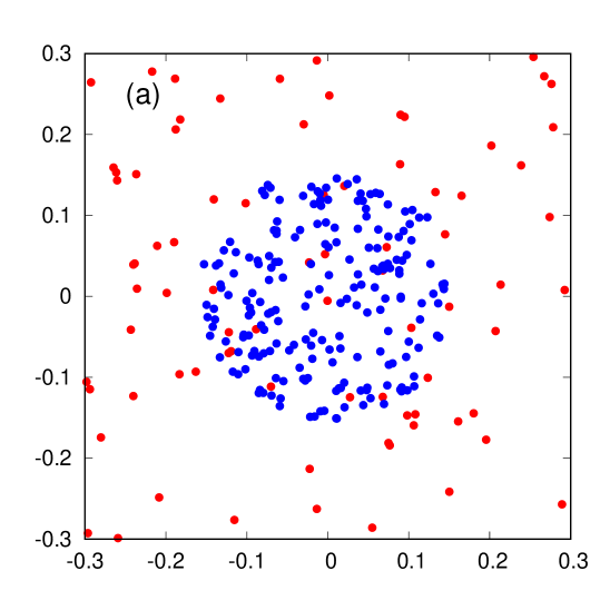
Figure 1: Simulation of $200$ cluster stars and $800$ field stars homogeneously distributed in a circular area of radius $1.0$, such as the cluster-field surface density ratio is $10$. (a) Distribution of stars in the central region: blue points are cluster stars and red points field stars. (b) The corresponding MST of the central region of the data sample. (c) The plotted convex hull surrounds the data points that the algorithm classifies as belonging to the overdensity (details in the text).

We adopt the working definition of a star cluster as an overdensity in a given phase-space diagram. Ideally, some kind of clustered structure should be seen for the full set of phase-space variables (positions, parallaxes, proper motions and radial velocities) but this is not always the case either because some of these variables are not available or because contamination by field stars hides the underlying clustered structure in some subspace. Here we consider only one set of two variables (proper motion). Let us assume there is a cluster inside a more spread distribution of field stars. The branch lengths of the MST constructed from the whole set of points should exhibit some kind of bimodal distribution with small branches corresponding to connections in the region of the diagram occupied by the cluster and large branches corresponding to connections among field stars. That is, the mean of the cluster branches should be, on average, smaller than the mean of the field branches.

For constructing the MST we use the Prim’s algorithm (Prim, 1957). At a given iterative step, we search for and add the smallest branch connecting points that are not part of the MST with points that are already part of the tree. If the starting point is a star in the cluster, the algorithm first adds to the tree stars belonging to the cluster (i.e. that are located in the high density region) because those stars are separated by the smallest distances. In an ideally-behaved case, field stars will be added to the MST only when all the cluster stars have been already included. At each step of the Prim’s algorithm, for the $N_{T}$ points that are part of the tree we calculate the mean length of the branches ($L_{T}$). If, for instance, we start from a star in the region covered by a nearly homogeneous cluster, we expect that $L_{T}$ remains approximately constant when we add cluster stars to the tree and it starts to increase when field stars with larger separations are included. This is the property we take advantage of to separate cluster from field.

A key point is the starting point. We are proceeding under the assumption that there is actually a cluster in the data sample. Our goal in this work is to derive the cluster radius and not to decide whether there is or not a cluster. The starting point can be set up by hand if the cluster position in the phase-space diagram is known. However, as we plan to apply this method massively and systematically to data from Gaia mission, we included a function in our code to automatically select as starting point the densest part of the tree, i.e. that with the maximum number of stars per unit length. To calculate the local density we consider a subsample of $N_{min}$ data points (see below the assumed value of this parameter). In any case, our tests showed that the method works well for any starting point as long as it is inside or close to the region occupied by the cluster.

2.1 Homogeneous cluster case

In order to understand how the method works, it is useful to see the results for a well-behaved cluster. For this we simulate two homogeneous distributions one of which is denser than the other (overdensity). Obviously this does not correspond to the case of two nearly gaussian distributions that we would expect in the proper motions space (we will show these simulations in Section 2.3), but this simple example case will serve to illustrate the main features and performance of the proposed method. The simulation consists of $1000$ stars randomly distributed in a circle of radius $1.0$ (arbitrary units), from which $200$ are cluster stars that are distributed in a denser region. The cluster-field surface density ratio is $10$. It is important to mention that for this simple ideal case the area covered by the overdensity in this phase-space overlaps with the cluster itself, but this will not be the case for more realistic clusters having radial density distributions (Section 2.3). In any case, some field stars are located by chance below the area occupied by cluster stars (Fig. 1a). Unless we use additional information from other physical variables, these stars will be incorrectly classified as cluster stars by this and any other method. If we construct the MST (Fig. 1b) starting from a cluster star and we plot mean length of the branches at each step we get what is shown in Fig. 2.

Figure 2: Mean length of the branches ($L_{T}$) as a function of the number of points that are part of the MST ($N_{T}$) for the simulated data shown in Fig. 1. Open circle indicates the point where the transition cluster-field occurs (see text).

At the beginning of constructing the MST we see some statistical fluctuations for low values of $N_{T}$, but after that $L_{T}$ remains fairly constant around the average separation of cluster stars in the phase-space diagram. After including all the $200$ cluster stars (plus some additional field stars below the cluster), $L_{T}$ begins to increase as new longer branches corresponding to the field are added to the MST. The transition from cluster to field is easily visible in Fig. 2 and it is the key property we use to separate cluster from field. We consider as cluster all the stars that are part of the MST at the transition point in the $L_{T}-N_{T}$ plot (open circle in Fig. 2). The convex hull containing these points (Fig. 1c) shows that the selection is done properly.

Figure 3: Results for simulation shown in Fig. 1. (a) Inclination angles in degrees ($\alpha$) for the cluster (solid line) and field (dashed line). (b) The corresponding values of the parameter $\eta$ (for clarity only the region $100\leq N_{T}\leq 300$ is shown).

This procedure is similar to the algorithm applied by Gutermuth et al. (2009) to extract YSO cores using Spitzer data (see also Koenig et al., 2008; Beuret et al., 2017). They used the cumulative distribution of branch lengths which were fitted to two or three lines to find the transition point. Our tests have shown that the mean branch length works better than the cumulative length to detect the transition in certain extreme cases, as for instance samples with low density contrast between cluster and background. Moreover, contrary to the above mentioned works, we do not need to define a cut-off length to determine the cluster radius.

2.2 The transition parameter $\eta$

If a cluster appears as an overdensity in the proper-motion vector point diagram then a cluster-field transition point should be discernible in a $L_{T}-N_{T}$ plot, although its exact shape and strength depend on the data sample (see Section 2.3). Our tests on both simulated and real data indicate that in the cases of overdensities visible by eye in the proper-motion vector point diagram the corresponding transition point is also clearly visible. For the sake of a fully automatic data processing we developed a subroutine to detect the transition point. First, we normalize $L_{T}$ and $N_{T}$ between $0$ and $1$ in order to make a data-independent analysis. Second, we fit straight lines to the left and right sides of the possible transition point. We require a minimum of $N_{min}$ data points for the left-side fitting to avoid noisy data effects. For the right-side fitting we use only the first $N_{min}$ data points because in general we do not expect a simple straight-line behaviour. From here we calculate the inclination angles of the left-side ($\alpha_{c}$) and right-side ($\alpha_{f}$) fits. What we do is to span all the possible transition points ($N_{T}$ values) and to search for the point where $\alpha_{f}-\alpha_{c}$ is maximum while $\alpha_{c}$ is minimum. The best theoretical expected transition would be when $\alpha_{f}=\alpha_{max}$ ($90$ deg or $\pi/2$ rad) and $\alpha_{c}=0$ deg. We define the dimensionless parameter

$$\eta=\frac{(\alpha_{f}-\alpha_{c})}{\max\{\alpha_{c},\delta\}}\times\frac{\delta}{\alpha_{max}}$$ (1)

that “quantifies" the sharpness of the transition with a value between $0$ (no transition) and $1$ (maximal transition). The arbitrary constant $\delta$ is introduced only to prevent the singularity when $\alpha_{c}=0$. Our tests on simulated data indicate that, although the exact value of $\delta$ affect the maximum of $\eta$ ($\eta_{max}$), it has very little effect on the position of that maximum, that is on the $N_{T}$ value at which the maximum occurs, as long as $\delta$ is small compared with $\alpha_{max}$. Here we are using $\delta=0.01\alpha_{max}$. We must point out that the functional form of $\eta$ is arbitrary, but this is not really relevant as long as we get the cluster-field transition point. The relevance of quantifying in some way the strength of the transition is to compare solutions obtained with different subsamples from the same dataset (Section 2.4).

Fig. 3 shows the inclination angles $\alpha_{c}$ (solid line) and $\alpha_{f}$ (dashed line) and the corresponding $\eta$ values for the well-behaved simulation shown in Figs. 1 and 2. For $N_{T}\gtrsim 300$ we see that $\alpha_{c}>\alpha_{f}$ (negative values for $\eta$). There is a relatively narrow region around $N_{T}\sim 200$ with valid solutions for which we can clearly see that $\alpha_{f}-\alpha_{c}$ is high whereas $\alpha_{c}\simeq 0$. The optimal solution (that with the maximum $\eta$ value, see Fig. 3b) is not located exactly at the theoretical value $N_{T}=200$ because of contamination by field stars lying below the cluster region.

In the end, we have only one relevant free parameter: the minimum number of data points required to get “valid" measurements ($N_{min}$). Its exact value is not critical when constructing the MST because the method is almost insensitive to the starting point. However, $N_{min}$ is important because it determines the range of $N_{T}$ values in which $\eta$ is calculated. If we have a sample of $N_{dat}$ stars then $\eta$ can be calculated only in the range $N_{min}<N_{T}<N_{dat}-N_{min}$. This means that the algorithm will not find the optimal solution if the actual number of cluster star is, for instance, below or too close to $N_{min}$. A value around $\sim\sqrt{N_{dat}}$ would be a reasonable choice, assuming Poissonian statistics, but to be conservative and after several tests we have assumed $N_{min}=3\sqrt{N_{dat}}$. The fact of having only one relevant free parameter brings robustness to the algorithm because minimize its sensitivity to parameter variations.

2.3 Tests on simulated data

During the development of this algorithm we have performed a number of tests on simulated data. Simulations included scenarios with different sample sizes, geometrical shapes, radial density profiles and cluster-field density contrasts. In general the algorithm worked quite well for all the simulations. The shape in which stars are distributed (including filamentary distributions) does not affect the detection of the cluster-field transition point as long as the number of member stars is larger than $N_{min}$. Obviously, the method works better when the surface density of cluster stars ($\Sigma_{c}$) is significantly higher than the density of field stars ($\Sigma_{f}$). In fact, the density contrast $\Sigma_{c}/\Sigma_{f}$ is practically the only factor that determines the behaviour and performance of the proposed algorithm.

In this section we discuss some example simulations for the case in which cluster and field follow radial density distributions, such as is the case for most of the real proper motion distributions. Cluster and field stars were distributed according to 2-dimensional Gaussian distributions having standard deviations of $\sigma_{c}$ and $\sigma_{f}>\sigma_{c}$ (cluster more concentrated than field), respectively, and both centred on the same coordinate (this is the worst case, i.e. the most difficult to separate cluster from field). The tests performed using elliptical (rather than circular) distributions for the stars yielded essentially the same results and trends. The only relevant variable is the ratio $\sigma_{c}/\sigma_{f}$, strongly related to the inverse of the density contrast $\Sigma_{c}/\Sigma_{f}$. Fig. 4 shows an example for which $\sigma_{c}/\sigma_{f}=0.3$, equivalent to having an average density contrast in the central region (within one cluster standard deviation) of $\Sigma_{c}/\Sigma_{f}\sim 2$.

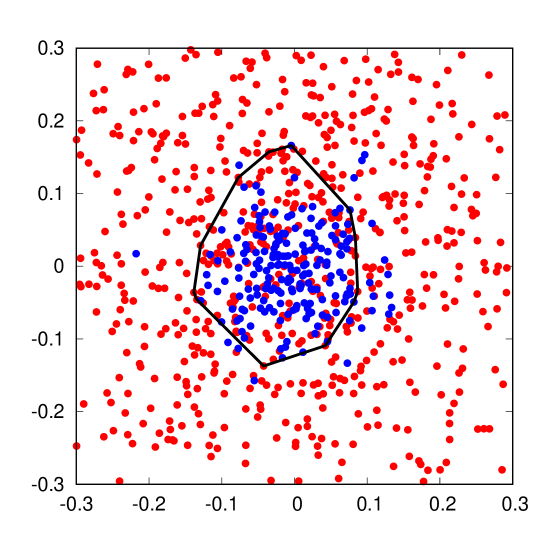
Figure 4: Simulation of $200$ cluster stars (blue points) and $800$ field stars (red points) following Gaussian density profiles. The ratio of standard deviations between cluster and field is $\sigma_{c}/\sigma_{f}=0.3$. For clarity, only the central region is shown (the whole area is circular with radius $1$). Solid line shows the final convex hull surrounding the selected overdensity.

The convex hull indicates the boundary of the overdensity according to the algorithm. As before, some field stars fall below the overdensity area and, additionally, some cluster stars at the edges of the distribution (where the local cluster density is around or below the field density at that point) are located outside the selected overdensity. We reiterate that this is not a limitation of the method but consequence of how the data sample is distributed, and can only be corrected by using additional spatial, kinematic or photometric information. In this work we do not intend to provide kinematic memberships. Our aim is to determine the cluster size in an objective and reliable manner as long as the cluster shows an overdensity in the proper motion space. Any cluster member we refer to is actually a star located in the overdensity region. Thus, at this point the algorithm selects the “best" boundary for a given overdensity, that is the boundary for which the most pronounced transition from short to long branches takes place.

In Fig. 5 we see the $\tilde{L}_{T}$-$N_{T}$ plot for some example simulations with radial density profiles going from a high density contrast to the no-cluster case.

Figure 5: Normalized mean length of the branches ($\tilde{L}_{T}$) as a function of the number of points in the MST ($N_{T}$) for four simulations with radial density distributions. For clarity an arbitrary offset have been added to the curves. The number of cluster and field stars are $N_{c}=200$ and $N_{f}=800$, respectively, but the simulations are for different cluster-to-field standard deviation ratios: $\sigma_{c}/\sigma_{f}=0.1$, $0.2$, $0.3$ and $1$. The corresponding average density contrasts (within a 1-$\sigma_{c}$ radius) are $\Sigma_{c}/\Sigma_{f}\sim 20$, $5$, $2$ and $1$, respectively. Open circles indicate the point where the algorithm selects the best cluster-field transition point. The cluster and field straight-line fits are also shown.

Differently to the homogeneous case (Fig. 2), the mean length of the branches increases as $N_{T}$ increases even for low $N_{T}$. However, the point with a notable change in the average slope is visible especially for the high contrast cases. Even when $\sigma_{c}/\sigma_{f}=0.3$ (low density contrast) the algorithm finds the transition point for $N_{T}=331$ which corresponds quite well to the overdensity observed in Fig. 4.

The simulation labelled $\sigma_{c}/\sigma_{f}=1$ corresponds to the case when there is no cluster but just one radial distribution of stars. This case exhibits random fluctuations from which the algorithm simply selects the strongest change in slope. This can be seen in Fig. 6 that shows $\eta$ for the high density contrast and no-cluster cases.

Figure 6: Transition parameter $\eta$ for simulations of radial distributions with two values of cluster-to-field standard deviation ratios: $\sigma_{c}/\sigma_{f}=0.1$ (solid line) and $\sigma_{c}/\sigma_{f}=1$ (dashed line).

Although the values of $\eta$ at high contrast are relatively low compared with the well-behaved, homogeneous distribution (see Fig. 3b), its maximum value clearly stands out at $N_{T}=169$. It is different for the no-cluster case (dashed line in Fig. 6) where the selected optimal transition at $N_{T}=301$ is not very different from other local maxima of $\eta$ around $N_{T}\sim 600$.

2.4 Estimation of cluster radius

It is not a simple task to determine (to define) the cluster radius in an objective way because the definition of radius is ambiguous itself given the great variety of observed morphologies. There are several commonly used characteristic radii, such as the core radius, half-mass (or half-light) radius, tidal radius, or simply the “extent" of the cluster usually defined as the radius where the cluster surface density drops below field density (the details depend on the author). Mixing these different concepts can lead to inaccurate or biased global results (see discussion in Pfalzner et al., 2016). Here we use the simple geometric definition of cluster radius as the radius of the smallest circle containing all the cluster stars. Following graph theory terminology we can refer to it as the covering radius ($R_{cov}$) to differentiate it of other characteristic radii. According to Sanchez et al. (2010) the sampling radius $R_{s}$ (i.e. the radius of the circular area around the cluster position used to extract the data from a given catalogue) that best discriminates kinematic members from field stars is $R_{s}=R_{cov}$. In this case an overdensity corresponding to the cluster’s centroid should be visible in the proper motion space. The procedure explained in the previous sections determines in a simple and direct way the area covered by this overdensity. For $R_{s}<R_{cov}$ the cluster is subsampled (by varying amounts, depending on cluster star density). On the contrary, for $R_{s}>R_{cov}$ only new field stars are included so that the cluster overdensity will be less prominent. The transition parameter defined in Section 2.2 quantitatively measures the sharpness of the overdensity. Thus, the strategy we follow is to apply an external loop over a range of $R_{s}$ values and, at each step calculate the maximum transition parameter $\eta_{max}$. We consider the optimal sampling radius as that with the highest of all the $\eta_{max}$ values. This optimal sampling radius is, as already discussed, the most reliable estimation of the actual cluster covering radius. Thus, this approach give us a method to calculate cluster radii directly from the data without making any additional assumptions about the spatial distribution of the cluster stars.

2.5 Estimation of uncertainties

The value of $\eta$ that determines the boundary of the overdensity ($\eta_{max}$) is unique for each given sampling radius $R_{s}$. We have estimated an uncertainty associated to each $\eta_{max}$ value using bootstrap techniques: we repeat the calculation on a series of random resamplings of the data, and the standard deviation of the obtained set of $\eta_{max}$-values is taken as the error in our estimation. Additionally, we use this error as a reference to estimate an overall uncertainty associated with the derived cluster radius. For this we define a lower limit given by the optimal solution (the highest of all the $\eta_{max}$ values) minus three times its standard deviation, and we assume that the range of acceptable solutions for the radius are all the values for which $\eta_{max}$ is above this lower limit (see Fig. 8 in next section for an example).

2.6 Test on NGC 188

The direct way of validating our method is to apply it to a well-known open cluster and compare the results. NGC 188 serves as a test case because it is old (and therefore it exhibits a clear radial density profile) and it is located far above the Galactic plane (with little contamination by field stars). NGC 188 has been extensively studied and it has relatively well-determined physical parameters (see Table 1 in Elsanhoury et al., 2016, for a summary of some published parameters). Regarding the cluster size, the radius reported in Dias et al. (2002) for NGC 188 is 8.5 arcmin, which is the value given in the WEBDA database (Mermilliod, 1995), whereas Kharchenko et al. (2013) estimated a relatively high value of 34.2 arcmin. Sampedro et al. (2017) determined a radius of 12 arcmin from its radial density profile. The characteristic scale most similar to what we call the covering radius is the limiting radius $R_{lim}$ defined as the radius that covers the cluster and reaches “enough" stability with the background (Tadross & Bendary, 2014). Bonatto et al. (2005) estimated $R_{lim}=24\pm 0.1$ arcmin for NGC 188, almost twice the last value of $R_{lim}=12.45$ arcmin given by Elsanhoury et al. (2016). These dissimilar values serve to exemplify the necessity of alternative approaches such as the one proposed here.

Figure 7: Radial density profile of stars toward NGC 188. Error bars are from Poisson statistics. Horizontal dashed line indicates the mean value of $0.51$ stars/arcmin² (plus/minus one standard deviation) estimated beyond $20$ arcmin.

In order to test the method with NGC 188 we extract its data (positions and proper motions) from the UCAC4 catalogue (Zacharias et al., 2013) in the same way that we will do with the rest of the cluster (Section 4). Figure 7 shows the corresponding radial density profile. Clearly the cluster density profile merges into the background at some point around $\sim 15$ arcmin (the exact value depending on the specific merging criterion).

Figure 8: Maximum value of the transition parameter ($\eta_{max}$) as a function of the sampling radius ($R_{s}$) for the open cluster NGC 188 (solid black line) with the vertical arrow indicating the obtained maximum. Grey shadow corresponds to one standard deviation computed using bootstrapping, whereas the horizontal dashed line indicates the maximum $\eta_{max}$ minus three standard deviations.

The result of applying our algorithm to NGC 188 is shown in Figure 8. For this well-behaved open cluster the maximum value of $\eta_{max}=0.16$ is found at $R_{s}=14.2$ arcmin, in very good agreement with its spatial density profile in Figure 7. As explained in Section 2.5, we associate an uncertainty to the calculated radius by considering all the $\eta_{max}$ that are above the dashed line in Figure 8. In this case the final cluster radio would be in the range $R_{c}=13.4-17.0$ arcmin.

In next sections we will apply this same procedure to a sample of open cluster with discrepant radius values in the literature.

3 Sample of clusters

We have compared the open cluster catalogues of Dias et al. (2002) and Kharchenko et al. (2013) (hereafter D02 and K13, respectively), both available via the VizieR database. The latest version (3.5 of 2016 February) of D02 contains updated information on $2167$ optically visible open clusters and candidates. Dias et al. (2014) used the UCAC4 catalogue (Zacharias et al., 2013) to determine in a homogeneous way kinematic memberships and mean proper motions for most of these clusters. However, the apparent radii of many of the clusters in D02 were compiled from older references (e.g. Lynga, 1987; Mermilliod, 1995) in which most of the apparent diameters were estimated from visual inspection. On the other hand, K13 used data from the PPMXL (Roeser et al., 2010) and 2MASS (Skrutskie et al., 2006) catalogues to calculate and provide a set of uniform astrophysical parameters for $3006$ clusters (most of them open clusters). They used multi-dimensional diagrams to determine combined (kinematic and photometric) membership probabilities for the stars (Kharchenko et al., 2012). They calculated cluster sizes fitting by eye the radial density profiles of the 1-$\sigma$ members. The fitting uses three empirical parameters: the radius of the core, of the central part and of the cluster. We take the last one, defined in K13 as the distance from the cluster centre where the surface density of members becomes equal to the average density of the field, as their estimation for the cluster radius. Cluster radius distributions for the full D02 and K13 catalogues exhibit an apparent bias with systematically higher cluster radii in K13 (that we will denote as $R_{K}$) than in D02 ($R_{D}$). The mean $R_{D}$ value is $\sim 7.2$ arcmin and the median $\sim 2.5$ arcmin, whereas the mean of $R_{K}$ is $\sim 10.5$ arcmin and the median $\sim 7.8$ arcmin.

In order to select a sample of clusters that were certainly common to both catalogues, we first matched each cluster in D02 with the closest cluster in K13, and then we kept only those with the same main name in both catalogues. These last step may accidentally discard some common clusters but in this way we are pretty sure we are comparing the same clusters. The matching yields $1706$ clusters whose radii are plotted in Fig. 9.

Figure 9: Cluster radius in the K13 catalogue ($R_{K}$) as a function of radius in D02 ($R_{D}$). All the clusters in common between both catalogues are shown as red points, cluster having more than $400$ expected members according to D02 are shown as blue points, and selected clusters are indicated with surrounding open circles. The solid line indicates the 1:1 line.

Again we can see that $R_{K}$ tends to be systematically higher than $R_{D}$, especially for small radius values ($R_{D}<3$ arcmin). We need a sufficiently high number of cluster stars to reach a valid solution ($N_{c}$ has to be greater than $N_{min}$). We do not know in advance $N_{c}$ but D02 give an estimation of the expected number of cluster members. They warn this can be an overestimate (our tests showed us that their estimations use to be $3-4$ times our final $N_{c}$ value), thus we additionally require the number of members estimated in D02 to be higher than $400$. The resulting $284$ clusters are shown as blue dots in Fig. 9. From here we select five clusters having extreme radii in the D02 and K13 catalogues: Ruprecht 175 (with the smallest $R_{K}$ value), NGC 6603 (the smallest $R_{D}$), NGC 1647 (the largest $R_{K}$), and ASCC 19 and Collinder 471 (the two largest $R_{D}$ values). A comparison of the cluster radii reported in D02 and K13, and the results obtained in this work is shown in Table 1.

Table 1: Properties of the selected clusters.

			Cluster radius
Name	RA	DEC	D02	K13	This work
	(h m s)	($\degr~{}\arcmin~{}\arcsec$)	(arcmin)	(arcmin)	(arcmin)
NGC 188	$00~{}47~{}28$	$+85~{}15~{}18$	8.5	34.2	15.2 $\pm$ 1.8
NGC 1647	$04~{}45~{}55$	$+19~{}06~{}54$	20.0	45.0	29.4 $\pm$ 3.4
ASCC 19	$05~{}27~{}47$	$-01~{}58~{}48$	48.0	31.2	…
NGC 6603	$18~{}18~{}26$	$-18~{}24~{}24$	3.0	8.4	4.2 $\pm$ 1.7
Ruprecht 175	$20~{}45~{}12$	$+35~{}30~{}00$	7.0	4.5	7.0 $\pm$ 0.3
Collinder 471	$22~{}07~{}06$	$+72~{}00~{}00$	65.0	8.4	…

4 Radius determination for the selected clusters

We use data from the UCAC4 catalogue (Zacharias et al., 2013) to apply the proposed method to the open clusters listed in Table 1. We extract proper motions for all the stars and clean the data leaving only “good" stars. We run the program spanning a wide range of sampling radius ($R_{s}$) values including both $R_{D}$ and $R_{K}$, with steps of $0.1-0.2$ arcmin.

4.1 NGC 1647

We will discuss in detail the first cluster of the selected sample (NGC 1647). Fig. 10 shows the obtained $\eta_{max}$ value for each sampling radius $R_{s}$.

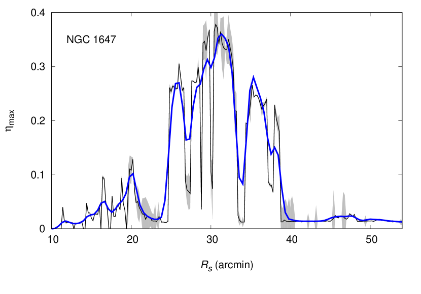
Figure 10: Maximum value of the transition parameter ($\eta_{max}$) as a function of the sampling radius ($R_{s}$) for the open cluster NGC 1647. The superimposed blue line is a smoothed curve obtained by using a Gaussian kernel (see text).

The first thing we note is that $\eta_{max}$ fluctuates with small variations in $R_{s}$. This is due to the functional form of the transition parameter (Eq. 1). The maximum $\eta$ values tend to occur for small values of $\alpha_{c}$ so that small $\alpha_{c}$ variations imply noticeable variations of $\eta$ (as can be seen in Figure 3). This effect will be more or less noticeable depending on the data itself and on how clear the overdensity can be seen in the proper motion space; for instance in NGC 188 these fluctuations are less apparent (Figure 8). Despite this, the overall trend is clearly discernible for NGC 1647, with some local maxima and an absolute maximum around $R_{s}\simeq 30$ arcmin. For a better visualization of the global behaviour we have superimposed a smoothed function (blue line in Fig. 10). The smoothing is done by convolving the data with a Gaussian kernel. According to Silverman (1986), the optimal bandwidth for $N$ normally distributed data points with standard deviation $\sigma$ is around $\sigma(4/3N)^{0.2}$, although this usually yields very conservative broad bandwidth so that we always use $1/10$ of the Silverman’s rule for the bandwidth. The most relevant transition cluster-field for NGC 1647 corresponds to $\eta_{max}=0.38$ at an optimal sampling radius of $R_{s}=30.6$ arcmin. Taking the uncertainty in $\eta_{max}$ into account our final estimation of the cluster radius is $R_{c}=26.0-32.8$ arcmin. The obtained radius is intermediate between the values given in D02 ($20$ arcmin) and K13 $R_{K}=45$ arcmin, and it agrees with the $30$ arcmin estimated by Geffert et al. (1996) from visual inspection of Palomar plates. In any case, beyond the associated uncertainties, Fig. 10 clearly rules out large values ($R_{C}\gtrsim 40$ arcmin) reported in other works (Piskunov et al., 2007, 2008; Sanchez & Alfaro, 2009; Kharchenko et al., 2013).

The particular results for three different sampling radii are compared in Fig. 11.

Figure 11: Normalized mean length of the branches $\tilde{L}_{T}$ as a function of the fraction of stars in the MST $N_{T}/N_{max}$ for the three indicated sampling radii. An arbitrary offset have been added to the curves. Open circles and solid lines indicated the best choices and the fits for the transition points.

Figure 12: Distribution of UCAC4 proper motions for the stars in the field of NGC 1647. (a) All the stars (red points) corresponding to the optimal sampling radius $R_{s}=30.6$ arcmin. Solid line is the convex hull surrounding the selected overdensity. (b) As in (a) but for $R_{s}=R_{D}=20$ arcmin. (c) Cluster members according to Dias et al. (2014) (they used $R_{s}=21$ arcmin). Blue points are star having membership probabilities higher than $50\%$ and black points have probabilities higher than $90\%$.

For a sampling radius of $R_{s}=R_{D}=20$ arcmin (the value given by D02) the sample consists of $722$ stars, from which the algorithm selects $N_{T}=86$ stars inside the overdensity area with a transition parameter of $\eta_{max}=0.15$. Instead, when $R_{s}=R_{K}=45$ arcmin (K13) the full sample is $2897$ with $N_{T}=348$ but, in this case, this is a relatively bad solution with $\eta_{max}=0.01$ as it can be easily seen by eye in Fig. 11 (an almost imperceptible transition for $R_{s}=45$ arcmin). For the optimal sampling radius ($30.6$ arcmin, this work) we obtain $N_{T}=155$ stars in the overdensity out of a total of $1464$ stars in the sample with a clearly detected transition ($\eta_{max}=0.38$). It is interesting to note that the fraction of overdensity stars is always around $N_{T}/N_{max}\sim 0.1$. This fact is an indicator of robustness of the method: the algorithm finds the area occupied by the overdensity, and when the sampling radius increases the number of contaminant stars also increases but the overdensity area remains nearly constant (see below) and $N_{T}/N_{max}$ changes very little. Fig. 12 shows proper motion distributions for two sampling radii: the optimal value found in this work (panel a) and that corresponding to the radius $R_{D}$ reported in D02 (panel b). By comparing panels a-b we see that the selected overdensity area is nearly the same even though the sampling radii are very different (the number of sample stars in panel a is twice that of panel b). This is not the case for the widely used method of fitting two Gaussian functions to represent the distributions of field and cluster stars (Vasilevskis et al., 1958; Sanders, 1971; Cabrera-Cano & Alfaro, 1985). In this case, when the sample is contaminated by many field stars the fit tends to produce a wider and flatter function for the field distribution and, as a consequence, the membership probabilities (defined as the ratio cluster-total distributions) increase and the number of spurious members also increases (this effect has been discussed in Sanchez et al., 2010). Panels b-c of Fig. 12 compare our results with those of Dias et al. (2014) (they used proper motions from UCAC4 to fit two elliptical bivariate Gaussian functions). As mentioned before our algorithm does not provide cluster memberships because this MST-based procedure only selects the area comprising the overdensity, although obviously the $155$ stars inside the convex hull are probable kinematic members of the cluster. There should be other additional members beyond the overdensity area where the cluster star density is around or below the local field star density. However, it is interesting to note that the number of overdensity stars is considerably smaller than the $459$ very probable members (membership probabilities $\geq 90\%$) according to Dias et al. (2014) (black points in Fig. 12) or than the $618$ 1-$\sigma$ members found by K13.

An excessively large number of spurious members can lead to inaccurate or biased estimations of open cluster proper motions (and other properties). Kurtenkov et al. (2016) used both kinematic and photometric criteria to select the most reliable members and recalculated proper motions for a sample of $15$ open clusters. For some of the clusters their results differ significantly from the ones given by Dias et al. (2014), and they suggested that the difference could be linked to a field star contamination effect. In the case of NGC 1647, Kurtenkov et al. (2016) calculated a proper motion $(\mu_{\alpha}\cos\delta,\mu_{\delta})=(-1.13,-1.27)$ mas yr^-1 whereas Dias et al. (2014) obtained $(\mu_{\alpha}\cos\delta,\mu_{\delta})=(-0.74,-0.57)$ mas yr^-1. Our cluster proper motion centroid $(\mu_{\alpha}\cos\delta,\mu_{\delta})=(-0.85,-1.11)$ mas yr^-1 is in between both values but slightly closer to the Kurtenkov et al. (2016) result ($|\Delta\mu|=0.32$ mas yr^-1). However, the error in proper motions ($\sim 1-4$ mas yr^-1) are similar to the errors given by Kurtenkov et al. (2016) and Dias et al. (2014) (limited by UCAC4 proper motion errors), so that theses differences are not significant.

4.2 The rest of the open clusters

The results for the remaining four clusters of Table 1 are shown in Fig. 13.

Figure 13: As in Fig. 10 but for the rest of the open clusters listed in Table 1.

We again see the same kind of fluctuations in $\eta_{max}$ as in Fig. 10. The smoothed (blue) curves allow to focus on global trends that we will comment on below.

ASCC 19:

This is a cluster reported as new by Kharchenko et al. (2005b) with a radius of $48$ arcmin (see also Piskunov et al., 2007) that it is the value given in D02. Afterwards, Kharchenko et al. (2013) recalculated a cluster radius of $31.2$ arcmin. We spanned a wide range of $R_{s}$ values but it has been not possible to find out a clear maximum for $\eta_{max}$. There are several local maxima with one of them slightly standing out at $\sim 49$ arcmin, a value very close to that in D02. We would like to point out that this unsuccessful outcome does not represent a “failure" of the method. For a given $R_{s}$ the algorithm recovers the overdensity in proper motions and the boundary that best delimits the cluster-field transition. The problem is that different sampling radii yield similar changes in slope. Thus, by using only kinematic data, we are not able to say what is the optimal sampling radius and, therefore, the cluster radius. This may be due, among others things, to the existence a more complex underlying patterns or simply to the lack of a clear overdensity in the proper motions space. An additional analysis including other physical variables (positions, photometry) should clarify this issue. We prefer to be conservative and say we did not find a feasible solution for ASCC 19. We use $R_{s}=49$ arcmin to show the proper motion distribution in Fig. 14.

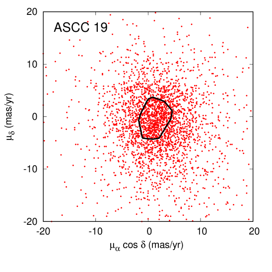
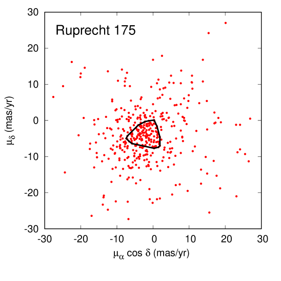
Figure 14: Proper motion distributions for the rest of the open clusters listed in Table 1 and for their optimal sampling radii (see text). Solid lines are the convex hulls surrounding the cluster members.

The number of data points for this radius is $2908$ from which $614$ corresponds to stars inside the convex hull. The proper motion centroid is at $(\mu_{\alpha}\cos\delta,\mu_{\delta})=(+1.20,-0.41)$ mas yr^-1 and it is not significantly different ($|\Delta\mu|=0.63$ mas yr^-1) from the value $(\mu_{\alpha}\cos\delta,\mu_{\delta})=(+1.43,-1.00)$ mas yr^-1 given by Dias et al. (2014).

NGC 6603:

For this cluster, the radius reported in the literature ranges from $R_{c}=2.8-3.0$ arcmin (Sagar & Griffiths, 1998; Dias et al., 2002) to $R_{c}=7.2-8.4$ arcmin (Kharchenko et al., 2005a, 2013). Our result (Fig. 13) points to some value in the range $R_{c}=2.5-5.9$ arcmin. There is another local maximum at around $\sim 9-10$ arcmin (very close to the value given by Kharchenko et al., 2013), but the former value is clearly the best solution. For a sampling radius at the center of the obtained range ($R_{s}=4.2$ arcmin) there are $595$ stars in the sample from which $123$ are part of the overdensity, whose calculated centroid is $(\mu_{\alpha}\cos\delta,\mu_{\delta})=(+0.67,-0.09)$ mas yr^-1, whereas Dias et al. (2014) reported $(\mu_{\alpha}\cos\delta,\mu_{\delta})=(+1.06,-0.72)$ mas yr^-1 ($|\Delta\mu|=0.74$ mas yr^-1).

Ruprecht 175:

We see two peaks at $R_{s}\simeq 4.1$ and $R_{s}\simeq 6.9$ arcmin, interestingly coinciding with the values $R_{K}=4.5$ and $R_{D}=7.0$ (Table 1). The highest is the second peak with $\eta_{max}=0.23$ which, with its associated uncertainty, yields a cluster radius of $R_{c}=6.7-7.3$ arcmin. The $119$ overdensity stars (out of $451$ stars for this sampling) have the centroid in $(\mu_{\alpha}\cos\delta,\mu_{\delta})=(-1.92,-3.90)$ mas yr^-1, whereas Dias et al. (2014)’s centroid is $(\mu_{\alpha}\cos\delta,\mu_{\delta})=(+2.60,-4.40)$ mas yr^-1 ($|\Delta\mu|=0.84$ mas yr^-1).

Collinder 471:

This is another extreme case in which we have a very large range of $R_{s}$ values to be spanned from $R_{K}=8.4$ arcmin to $R_{D}=65.0$ arcmin. The result is also a multi-peak plot but, in this case, values around $\sim 8.4$ arcmin are clearly ruled out. One of the local maxima is close to the radius reported by D02 but, again, there is not a clearly defined solution. For $R_{s}=65$ arcmin there are $5411$ stars with $327$ in the overdensity. The corresponding proper motion centroid is $(\mu_{\alpha}\cos\delta,\mu_{\delta})=(-1.57,-3.09)$ mas yr^-1 and Dias et al. (2014)’s centroid is $(\mu_{\alpha}\cos\delta,\mu_{\delta})=(-2.22,-3.32)$ mas yr^-1, ($|\Delta\mu|=0.69$ mas yr^-1). The shape of the proper motion distribution of members for Collinder 471 is rather elongated (see Fig. 14). This shape resembles the detection of substructures in the proper motion space of the open cluster NGC 2548 (Vicente et al., 2016). However, given that there is no a clear unique solution and that some spurious structures might appear when having such a large number of field stars in the sample ($\gtrsim 5000$) the existence of such elongated distribution is questionable. A more detailed analysis, beyond the scope of this study, would be necessary.

5 Conclusions

In this work we have presented a method for calculating cluster radii in a totally objective way. The MST is used to discriminate cluster from field in the proper motion space, and the quality of the separation is quantified. This is done for a range of sampling radii and the cluster radius is obtained as the radius at which the optimal performance is obtained. It is a different approach that does not make use of the spatial distribution of cluster stars (like when analysing radial density profiles). This makes the method particularly useful for irregular and/or poorly-populated open clusters.

In general, the obtained cluster radius may depend on the used astrometric catalogue, either because the way in which the catalogue is generated can produce some artefacts in the proper motion space, or because of the internal precision of the data. Here we have used UCAC4 proper motions to determine the radii of several open clusters, although we expect to analyse a larger sample of cluster with precise proper motions from Gaia. NGC 188, NGC 1647, NGC 6603 and Ruprecht 175 yielded unambiguous results. The obtained radii for NGC 188 and NGC 1647 are $R_{c}=15.2\pm 1.8$ and $R_{c}=29.4\pm 3.4$ arcmin, respectively, values more or less intermediate between the values given in D02 and K13. NGC 6603 and Ruprecht 175 have radii of $R_{c}=4.2\pm 1.7$ and $R_{c}=7.0\pm 0.3$ arcmin, respectively, values that are closer to D02’s values than to K13’s value. Finally, both ASCC 19 and Collinder 471 show a multi-peak behaviour and in these cases it is not possible to be confident about the right solution. It would be necessary to carry out additional tests in oder to know whether the multiple solutions for these clusters are consequence of the lack of a clear overdensity or of the occurrence of complex patterns in their proper motion distributions.

References

- Alfaro & González (2016) Alfaro, E. J., & González, M. 2016, MNRAS, 456, 2900
- Barrow et al. (1985) Barrow, J. D., Bhavsar, S. P., & Sonoda, D. H. 1985, MNRAS, 216, 17
- Beuret et al. (2017) Beuret, M., Billot, N., Cambrésy, L., et al. 2017, A&A, 597, A114
- Bonatto et al. (2005) Bonatto, C., Bica, E., & Santos, J. F. C., Jr. 2005, A&A, 433, 917
- Cabrera-Cano & Alfaro (1985) Cabrera-Cano, J., & Alfaro, E. J. 1985, A&A, 150, 298
- Cartwright & Whitworth (2004) Cartwright, A., & Whitworth, A. P. 2004, MNRAS, 348, 589
- Cartwright et al. (2006) Cartwright, A., Whitworth, A. P., & Nutter, D. 2006, MNRAS, 369, 1411
- de la Fuente Marcos & de la Fuente Marcos (2004) de la Fuente Marcos, R., & de la Fuente Marcos, C. 2004, New Astron., 9, 475
- Dias et al. (2002) Dias, W. S., Alessi, B. S., Moitinho, A., & Lépine, J. R. D. 2002, A&A, 389, 871
- Dias & Lépine (2005) Dias, W. S., & Lépine, J. R. D. 2005, ApJ, 629, 825
- Dias et al. (2014) Dias, W. S., Monteiro, H., Caetano, T. C., et al. 2014, A&A, 564, A79
- Dib et al. (2017) Dib, S., Schmeja, S., & Parker, R. J. 2017, arXiv:1707.00744
- Elsanhoury et al. (2016) Elsanhoury, W. H., Haroon, A. A., Chupina, N. V., et al. 2016, New Astron., 49, 32
- Geffert et al. (1996) Geffert, M., Bonnefond, P., Maintz, G., & Guibert, J. 1996, A&AS, 118, 277
- Gilmore et al. (2012) Gilmore, G., Randich, S., Asplund, M., et al. 2012, The Messenger, 147, 25
- Gregorio-Hetem et al. (2015) Gregorio-Hetem, J., Hetem, A., Santos-Silva, T., & Fernandes, B. 2015, MNRAS, 448, 2504
- Gutermuth et al. (2009) Gutermuth, R. A., Megeath, S. T., Myers, P. C., et al. 2009, ApJS, 184, 18
- Jaffa et al. (2017) Jaffa, S. E., Whitworth, A. P., & Lomax, O. 2017, MNRAS, 466, 1082
- Kharchenko et al. (2005a) Kharchenko, N. V., Piskunov, A. E., Röser, S., Schilbach, E., & Scholz, R.-D. 2005a, A&A, 438, 1163
- Kharchenko et al. (2005b) Kharchenko, N. V., Piskunov, A. E., Röser, S., Schilbach, E., & Scholz, R.-D. 2005b, A&A, 440, 403
- Kharchenko et al. (2012) Kharchenko, N. V., Piskunov, A. E., Schilbach, E., Röser, S., & Scholz, R.-D. 2012, A&A, 543, A156
- Kharchenko et al. (2013) Kharchenko, N. V., Piskunov, A. E., Schilbach, E., Röser, S., & Scholz, R.-D. 2013, A&A, 558, A53
- Koenig et al. (2008) Koenig, X. P., Allen, L. E., Gutermuth, R. A., et al. 2008, ApJ, 688, 1142-1158
- Krone-Martins & Moitinho (2014) Krone-Martins, A., & Moitinho, A. 2014, A&A, 561, A57
- Kurtenkov et al. (2016) Kurtenkov, A., Dimitrova, N., Atanasov, A., & Aleksiev, T. D. 2016, Research in Astronomy and Astrophysics, 16, 105
- Lomax et al. (2011) Lomax, O., Whitworth, A. P., & Cartwright, A. 2011, MNRAS, 412, 627
- Lynga (1987) Lynga, G. 1987, Computer Based Catalogue of Open Cluster Data, 5th edn. (Strasbourg: CDS)
- Mermilliod (1995) Mermilliod, J.-C. 1995, Information and On-Line Data in Astronomy, 203, 127
- Moraux (2016) Moraux, E. 2016, EAS Publications Series, 80, 73
- Netopil et al. (2015) Netopil, M., Paunzen, E., & Carraro, G. 2015, A&A, 582, A1
- Pfalzner et al. (2016) Pfalzner, S., Kirk, H., Sills, A., et al. 2016, A&A, 586, A68
- Perren et al. (2015) Perren, G. I., Vázquez, R. A., & Piatti, A. E. 2015, A&A, 576, A6
- Piskunov et al. (2007) Piskunov, A. E., Schilbach, E., Kharchenko, N. V., Röser, S., & Scholz, R.-D. 2007, A&A, 468, 151
- Piskunov et al. (2008) Piskunov, A. E., Schilbach, E., Kharchenko, N. V., Röser, S., & Scholz, R.-D. 2008, A&A, 477, 165
- Prim (1957) Prim, R. C. 1957, Bell System Technical Journal 36, 1389
- Randich et al. (2013) Randich, S., Gilmore, G., & Gaia-ESO Consortium 2013, The Messenger, 154, 47
- Roeser et al. (2010) Roeser, S., Demleitner, M., & Schilbach, E. 2010, AJ, 139, 2440
- Sagar & Griffiths (1998) Sagar, R., & Griffiths, W. K. 1998, MNRAS, 299, 1
- Sampedro et al. (2017) Sampedro, L., Dias, W. S., Alfaro, E. J., Monteiro, H., & Molino, A. 2017, MNRAS, 470, 3937
- Sanchez & Alfaro (2009) Sanchez, N., & Alfaro, E. J. 2009, ApJ, 696, 2086
- Sanchez et al. (2010) Sanchez, N., Vicente, B., & Alfaro, E. J. 2010, A&A, 510, A78
- Sanders (1971) Sanders, W. L. 1971, A&A, 14, 226
- Sarro et al. (2014) Sarro, L. M., Bouy, H., Berihuete, A., et al. 2014, A&A, 563, A45
- Schmeja & Klessen (2006) Schmeja, S., & Klessen, R. S. 2006, A&A, 449, 151
- Schmeja et al. (2008) Schmeja, S., Kumar, M. S. N., & Ferreira, B. 2008, MNRAS, 389, 1209
- Silverman (1986) Silverman, B. W. 1986, Density Estimation for Statistics and Data Analysis. London: Chapman & Hall/CRC. p. 48. ISBN 0-412-24620-1
- Skrutskie et al. (2006) Skrutskie, M. F., Cutri, R. M., Stiening, R., et al. 2006, AJ, 131, 1163
- Tadross & Bendary (2014) Tadross, A. L., & Bendary, R. 2014, Journal of Korean Astronomical Society, 47, 137
- Vasilevskis et al. (1958) Vasilevskis, S., Klemola, A., & Preston, G. 1958, AJ, 63, 387
- Vicente et al. (2016) Vicente, B., Sánchez, N., & Alfaro, E. J. 2016, MNRAS, 461, 2519
- Wang et al. (2016) Wang, K., Testi, L., Burkert, A., et al. 2016, ApJS, 226, 9
- Zacharias et al. (2013) Zacharias, N., Finch, C. T., Girard, T. M., et al. 2013, AJ, 145, 44