Asymptotic Properties for Markovian Dynamics in Quantum Theory and General Probabilistic Theories

Abstract

We address asymptotic decoupling in the context of Markovian quantum dynamics. Asymptotic decoupling is an asymptotic property on a bipartite quantum system, and asserts that the correlation between two quantum systems is broken after a sufficiently long time passes. The first goal of this paper is to show that asymptotic decoupling is equivalent to local mixing which asserts the convergence to a unique stationary state on at least one quantum system. In the study of Markovian dynamics, mixing and ergodicity are fundamental properties which assert the convergence and the convergence of the long-time average, respectively. The second goal of this paper is to show that mixing for dynamics is equivalent to ergodicity for the two-fold tensor product of dynamics. This equivalence gives us a criterion of mixing that is a system of linear equations. All results in this paper are proved in the framework of general probabilistic theories (GPTs), but we also summarize them in quantum theory.

,

• June 2019

Keywords: Markovian dynamics, asymptotic decoupling, mixing, ergodicity, $C_{0}$ semigroup, tensor product, quantum theory, general probabilistic theories

1 Introduction

Decoupling asserts that a quantum channel breaks the correlation between two quantum systems, and attracts attention in open quantum systems [1] and quantum information [4, 2, 3]. For example, Dupuis et al. [3] proved a decoupling theorem and clarified a relation between the accuracy of decoupling and conditional entropies. Since the correlation between two quantum systems should be small for instance in evaluating information leakage [5, 6], it is an interesting topic to investigate decoupling in the context of quantum dynamics. In this paper, we introduce asymptotic decoupling in the context of Markovian quantum dynamics, and clarify a necessary and sufficient condition of asymptotic decoupling. By our necessary and sufficient condition, asymptotic decoupling is closely related to another fundamental property in the study of Markovian dynamics.

Markovian dynamics has been often discussed in the context of statistical mechanics [7, 8, 9]. In such studies, it is important how an initial state changes after a sufficiently long time passes. In particular, the convergence (called mixing) and the convergence of the long-time average (called ergodicity) interest many researchers [10, 11]. More precisely, mixing asserts that, for any initial state, the state at discrete time $n$ (continuous time $t$) converges to a unique stationary state as $n\to\infty$ ($t\to\infty$); ergodicity asserts that, for any initial state, the long-time average converges to a unique stationary state. Hence mixing and ergodicity have been discussed in the context of relaxation to thermal equilibrium [7, 8, 9]. However, beyond the study of relaxation processes, these properties have found important applications in several fields of quantum information theory. In particular, in quantum control [12], quantum estimation [13], quantum communication [14], and the study of efficient tensorial representations of critical many-body quantum systems [15]. Ergodicity can be checked by solving a system of linear equations [10, 11], but a well-known criterion of mixing requires us to solve an eigenequation [10]. Thus mixing is clearly different from ergodicity with respect to their definitions and numerical checks. In this paper, we show that mixing for dynamics is equivalent to ergodicity for the two-fold tensor product of dynamics. It enables us to check mixing by solving a system of linear equations. Furthermore, asymptotic decoupling is equivalent to local mixing which asserts the convergence to a unique stationary state on at least one quantum system.

As a simple application of the above result, we give a relation between irreducibility and primitivity which are important properties in Perron-Frobenius theory. Irreducibility and primitivity guarantee the existence of Perron-Frobenius eigenvalues, which play an important roll in analyzing hidden Markovian processes [16, 17]. For example, Perron-Frobenius eigenvalues characterize the asymptotic performance of the average of observed values in a classical hidden Markovian process: the central limit theorem, large deviation, and moderate deviation [16]. The same method can be applied to a hidden Markovian process with a quantum hidden system [17]. For the above importance, we address irreducibility and primitivity. Since irreducibility and primitivity are close to ergodicity and mixing respectively, irreducibility for dynamics is equivalent to primitivity for the two-fold tensor product of dynamics. Using this equivalence, we obtain many conditions equivalent to primitivity, since there are many conditions equivalent to irreducibility.

In general, quantum dynamics is composed of quantum channels given as trace-preserving and completely positive linear maps (TP-CP maps). However, in order to handle stochastic operation including stochastic local operation and classical communication (SLOCC), we need to address quantum channels without trace-preserving. Fortunately, most results in this paper do not require trace-preserving. Also, complete positivity is not necessarily required and positivity is required. Therefore, we show our results for positive maps mainly.

So far, we have stated the asymptotic properties in the context of Markovian classical/quantum dynamics, but our results hold in the framework of general probabilistic theories (GPTs). GPTs are a general framework including quantum theory and classical probability theory [18, 19, 20]. Although quantum theory is widely accepted in current physics, more general requirements based on states and measurements only imply GPTs and do not imply quantum theory uniquely. Hence some researchers in physics study GPTs to explore conditions characterizing quantum theory. Since our results hold in GPTs, the asymptotic properties for Markovian dynamics do not require the framework of quantum theory and are common properties in GPTs. GPTs enable us to be easily address Markovian quantum dynamics composed of (not necessarily CP) positive maps. Therefore, our results are proved in the framework of GPTs after the quantum version of our results is stated in Section 2. Furthermore, due to the generality of our setting, our result can be used to investigate the structure of linear maps with the invariance of a cone, which is studied in Perron-Frobenius theory.

The remaining is organized as follows. Section 2 is a summary of results in Section 5 in the quantum case. As preparation for later discussion, Section 3 describes the framework of GPTs. Section 4 characterizes dynamical maps in the framework of GPTs. In this framework, Sections 5.1–5.3 state our results on asymptotic properties for Markovian dynamics with discrete-time, namely, asymptotic decoupling, mixing, and ergodicity. Section 5.4 proceeds to the continuous case, and show the same results as the discrete case by using results of discrete-time evolution. Section 6 gives a simple application of a result in Section 5.3 to Perron-Frobenius theory. Section 7 is our conclusion.

2 Summary of our results in quantum theory

We summarize results in Section 5 in the quantum case. First, we remark on quantum channels which compose Markovian quantum dynamics. In quantum theory, quantum channels are given as TP-CP maps on the set $\mathcal{T}(\mathcal{H})$ of all Hermitian matrices on a finite-dimensional quantum system $\mathcal{H}$. The set $\mathcal{T}(\mathcal{H})$ can be regarded as a finite-dimensional real Hilbert space equipped with the Hilbert-Schmidt inner product $\braket{X,Y}=\Tr XY$. In particular, quantum channels are given as linear maps on $\mathcal{T}(\mathcal{H})$. Most results in this paper only require linearity and positivity, but for simplicity we focus on only TP-CP maps in this section.

Next, let us introduce some notations on a bipartite quantum system $\mathcal{H}_{1}\otimes\mathcal{H}_{2}$. Throughout this paper, we use tilde to express to be bipartite. For instance, a bipartite quantum state is denoted by $\tilde{\rho}$, and a bipartite quantum channel is denoted by $\tilde{\Gamma}$. For a number $i\in\{1,2\}$ and a quantum state $\tilde{\rho}$ on $\mathcal{H}_{1}\otimes\mathcal{H}_{2}$, the reduced state on $\mathcal{H}_{i}$ of $\tilde{\rho}$ is denoted by $\pi_{i}(\tilde{\rho})$. That is, by using the partial traces $\Tr_{1}$ and $\Tr_{2}$, we have $\pi_{1}(\tilde{\rho})=\Tr_{2}\tilde{\rho}$ and $\pi_{2}(\tilde{\rho})=\Tr_{1}\tilde{\rho}$.

2.1 Discrete-time evolution

As Figure 1, let us consider dynamics when a quantum channel $\Gamma$ is applied to an initial quantum state $\rho$ many times. Then the dynamics is Markovian and discrete-time evolution. Now, in the bipartite case, we are interested in the asymptotic behavior of the $n$-th state $\tilde{\Gamma}^{n}(\tilde{\rho})$ as $n\to\infty$, and especially interested in whether the correlation between two quantum systems vanishes asymptotically. If the correlation vanishes asymptotically, we say that $\tilde{\Gamma}$ is asymptotically decoupling. Mathematically, asymptotic decoupling is defined as follows:

Figure 1: Markovian quantum dynamics with discrete-time.

Definition 2.1 (Asymptotic decoupling).

A quantum channel $\tilde{\Gamma}$ is asymptotically decoupling if any state $\tilde{\rho}$ satisfies

$$\tilde{\Gamma}^{n}(\tilde{\rho})=\pi_{1}(\tilde{\Gamma}^{n}(\tilde{\rho}))\otimes\pi_{2}(\tilde{\Gamma}^{n}(\tilde{\rho}))+o(1)\quad(n\to\infty).$$

Since the above right-hand side is a product state, it means to be no correlation. Next, to clarify a necessary and sufficient condition of asymptotic decoupling, we introduce another asymptotic property, namely, mixing:

Definition 2.2 (Mixing).

A quantum channel $\Gamma$ is mixing if there exists a state $\rho_{0}$ such that any state $\rho$ satisfies

$$\lim_{n\to\infty}\Gamma^{n}(\rho)=\rho_{0}.$$ (1)

The state $\rho_{0}$ is called the stationary state.

By using the above term, let us give a necessary and sufficient condition of asymptotic decoupling. For simplicity, first, we give it for a tensor product quantum channel $\Gamma_{1}\otimes\Gamma_{2}$:

Theorem 2.3.

For any two quantum channels $\Gamma_{1}$ and $\Gamma_{2}$, the following conditions are equivalent.

1. $\Gamma_{1}\otimes\Gamma_{2}$ is asymptotically decoupling.

2. $\Gamma_{1}$ or $\Gamma_{2}$ at least one is mixing.

Condition (2) can be represented as a simple phrase local mixing. Hence, simply speaking, asymptotic decoupling is equivalent to local mixing. Since spectral criterion [10, Theorem 7] is known as a criterion of mixing, the computation of eigenequations determines whether a tensor product quantum channel is asymptotically decoupling or not. These are why Theorem 2.3 is simple and meaningful. Moreover, the above equivalence also holds for a general quantum channel:

Theorem 2.4.

For any quantum channel $\tilde{\Gamma}$, the following conditions are equivalent.

1. $\tilde{\Gamma}$ is asymptotically decoupling.

2. There exist a number $i_{1}\in\{1,2\}$ and a state $\rho_{0,i_{1}}$ on $\mathcal{H}_{i_{1}}$ such that any state $\tilde{\rho}$ satisfies

   $$\tilde{\Gamma}^{n}(\tilde{\rho})=\rho_{0,i_{1}}\otimes\pi_{i_{2}}(\tilde{\Gamma}^{n}(\tilde{\rho}))+o(1)\quad(n\to\infty),$$

   where $i_{2}$ is an element of $\{1,2\}$ except for $i_{1}$.

Condition (2) can be explicitly written as

Case $(i_{1},i_{2})=(1,2)$   

$\tilde{\Gamma}^{n}(\tilde{\rho})=\rho_{0,1}\otimes\pi_{2}(\tilde{\Gamma}^{n}(\tilde{\rho}))+o(1)$,

Case $(i_{1},i_{2})=(2,1)$   

$\tilde{\Gamma}^{n}(\tilde{\rho})=\pi_{1}(\tilde{\Gamma}^{n}(\tilde{\rho}))\otimes\rho_{0,2}+o(1)$.

Since the state $\rho_{0,1}$ or $\rho_{0,2}$ is something like a stationary state, condition (2) can also be regarded as local mixing. Hence, for a general quantum channel, the same simple equivalence also holds: asymptotic decoupling is equivalent to local mixing.

For the above equivalence, it is meaningful to investigate a necessary and sufficient condition of mixing. Of course, as already mentioned, spectral criterion [10, Theorem 7] is known as a criterion of mixing, but it requires us to solve an eigenequation. Hence, let us give another criterion of mixing that is a system of linear equations. For this purpose, we introduce another asymptotic property, namely, ergodicity:

Definition 2.5 (Ergodicity).

A quantum channel $\Gamma$ is ergodic if there exists a state $\rho_{0}$ such that any state $\rho$ satisfies

$$\lim_{t\to\infty}\frac{1}{n}\sum_{k=0}^{n-1}\Gamma^{k}(\rho)=\rho_{0}.$$ (2)

The state $\rho_{0}$ is called the stationary state.

Since the right-hand side of (2) is the Cesàro mean of the right-hand side of (1), mixing implies ergodicity, but the converse does not necessarily hold. Definition 2.5 cannot be checked directly by computing, but its numerical check is realized by the following proposition:

Proposition 2.6.

For any quantum channel $\Gamma$, the following conditions are equivalent.

1. $\Gamma$ is ergodic.

2. $\dim\operatorname{Ker}(\Gamma-\operatorname{id}_{\mathcal{T}(\mathcal{H})})=1$.

The symbol $\operatorname{id}_{\mathcal{T}(\mathcal{H})}$ denotes the identity map on $\mathcal{T}(\mathcal{H})$.

Actually, as proved in Section 5.3, a quantum channel $\Gamma$ is mixing if and only if $\Gamma^{\otimes 2}$ is ergodic. This equivalence and Proposition 2.6 imply the following theorem which achieves the second goal of this paper:

Theorem 2.7.

For any quantum channel $\Gamma$, the following conditions are equivalent.

1. $\Gamma$ is mixing.

2. $\Gamma^{\otimes 2}$ is mixing.

3. $\Gamma^{\otimes 2}$ is ergodic.

4. $\dim\operatorname{Ker}(\Gamma^{\otimes 2}-\operatorname{id}_{\mathcal{T}(\mathcal{H}^{\otimes 2})})=1$.

Proposition 2.6 is well-known (for instance, see [10, appendix], [11, Corollary 2]), but Theorem 2.7 is not fully known as far as we know, and only partial results are published. For instance, the equivalence of conditions (1) and (3) in Theorem 2.7 was proved for unital quantum channels in finite-dimensions [21, Theorem 2.10]. An equivalence of conditions similar to conditions (1) and (3) is known for unital normal CP maps in infinite-dimensions [22, Theorem 6.3]. However, only a few preceding studies considered tensor product channels in the first place [21, 22, 23]. Their proofs are of operator algebra, but our proof is of linear algebra, and thus Theorem 2.7 also holds in GPTs.

Finally, summarizing Theorems 2.3 and 2.7, we have the following theorem immediately:

Theorem 2.8.

Let $\Gamma_{1}$ and $\Gamma_{2}$ be quantum channels. If $\Gamma_{2}$ is not mixing, then the following conditions are equivalent.

1. $\Gamma_{1}$ is mixing.

2. $\Gamma_{1}^{\otimes 2}$ is mixing.

3. $\Gamma_{1}^{\otimes 2}$ is ergodic.

4. $\dim\operatorname{Ker}(\Gamma_{1}^{\otimes 2}-\operatorname{id}_{\mathcal{T}(\mathcal{H}_{1}^{\otimes 2})})=1$.

5. $\Gamma_{1}\otimes\Gamma_{2}$ is asymptotically decoupling.

2.2 Continuous-time evolution

Next, we address continuous-time evolution. In the discrete case, $\Gamma^{n}(\rho)$ has denoted the state at time $n\in\mathbb{N}$. Since we address continuous-time evolution in this subsection, we denote by $\Gamma^{(t)}(\rho)$ the state at time $t>0$. Moreover, it is natural that the family $\{\Gamma^{(t)}\}_{t>0}$ of quantum channels should satisfy

• $\Gamma^{(t)}\circ\Gamma^{(s)}=\Gamma^{(t+s)}$ for all $t,s>0$,

• $\Gamma^{(t)}\to\operatorname{id}_{\mathcal{T}(\mathcal{H})}$ as $t\downarrow 0$.

The above first condition is illustrated by Figure 2. It asserts that the state at time $t+s$ equals the state after a time $s$ passes from the state at time $t$. A family $\{\Gamma^{(t)}\}_{t>0}$ satisfying the above two conditions is called a $C_{0}$ semigroup. It can be easily checked that any $C_{0}$ semigroup $\{\Gamma^{(t)}\}_{t>0}$ is right-continuous everywhere. The definition of a $C_{0}$ semigroup is simple and intuitive in the finite-dimensional case, but the infinite-dimensional case needs a few technical conditions. Although there are many studies on $C_{0}$ semigroups of finite/infinite-dimensions, we use no existing results on $C_{0}$ semigroups and only use the above two conditions. In the context of Markovian quantum dynamics, $C_{0}$ semigroups are also called quantum dynamical semigroups [26].

Figure 2: Markovian quantum dynamics with continuous-time.

In order to state our results in the continuous case, we need to define the continuous versions of asymptotic decoupling, mixing, and ergodicity. Fortunately, once replacing $\Gamma^{n}$ and $n\to\infty$ with $\Gamma^{(t)}$ and $t\to\infty$ respectively, the continuous versions of asymptotic decoupling and mixing are defined. However, to define the continuous version of ergodicity, we need to use an integral as follows:

Definition 2.9 (Ergodicity).

A $C_{0}$ semigroup $\{\Gamma^{(t)}\}_{t>0}$ is ergodic if there exists a state $\rho_{0}$ such that any state $\rho$ satisfies

$$\lim_{t\to\infty}\frac{1}{t}\int_{0}^{t}\Gamma^{(s)}(\rho)\,ds=\rho_{0}.$$

The state $\rho_{0}$ is called the stationary state.

Any mixing $C_{0}$ semigroup $\{\Gamma^{(t)}\}_{t>0}$ is ergodic in the same way as the discrete case. This fact is due to L’Hospital’s rule. In the above setting, our results are below:

Theorem 2.10.

For any two $C_{0}$ semigroups $\{\Gamma_{1}^{(t)}\}_{t>0}$ and $\{\Gamma_{2}^{(t)}\}_{t>0}$, the following conditions are equivalent.

1. $\{\Gamma_{1}^{(t)}\otimes\Gamma_{2}^{(t)}\}_{t>0}$ is asymptotically decoupling.

2. $\{\Gamma_{1}^{(t)}\}_{t>0}$ or $\{\Gamma_{2}^{(t)}\}_{t>0}$ at least one is mixing.

Theorem 2.11.

For any $C_{0}$ semigroup $\{\tilde{\Gamma}^{(t)}\}_{t>0}$, the following conditions are equivalent.

1. $\{\tilde{\Gamma}^{(t)}\}_{t>0}$ is asymptotically decoupling.

2. There exist a number $i_{1}\in\{1,2\}$ and a state $\rho_{0,i_{1}}$ on $\mathcal{H}_{i_{1}}$ such that any state $\tilde{\rho}$ satisfies

   $$\tilde{\Gamma}^{(t)}(\tilde{\rho})=\rho_{0,i_{1}}\otimes\pi_{i_{2}}(\tilde{\Gamma}^{(t)}(\tilde{\rho}))+o(1)\quad(t\to\infty),$$

   where $i_{2}$ is an element of $\{1,2\}$ except for $i_{1}$.

Theorem 2.12.

For any $C_{0}$ semigroup $\{\Gamma^{(t)}\}_{t>0}$, the following conditions are equivalent.

1. $\{\Gamma^{(t)}\}_{t>0}$ is mixing.

2. $\{(\Gamma^{(t)})^{\otimes 2}\}_{t>0}$ is mixing.

3. $\{(\Gamma^{(t)})^{\otimes 2}\}_{t>0}$ is ergodic.

4. $\Gamma^{(\epsilon)}$ is mixing for some $\epsilon>0$.

5. $(\Gamma^{(\epsilon)})^{\otimes 2}$ is mixing for some $\epsilon>0$.

6. $(\Gamma^{(\epsilon)})^{\otimes 2}$ is ergodic for some $\epsilon>0$.

Similarly to the discrete case, asymptotic decoupling is equivalent to local mixing, and mixing for dynamics is equivalent to ergodicity for the two-fold tensor product of dynamics.

Some readers might consider that Theorems 2.10, 2.11, and 2.12 are more general than Theorems 2.3, 2.4, and 2.7. However, it is not true due to the following reason. Any $C_{0}$ semigroup $\{\Gamma^{(t)}\}_{t>0}$ can be represented as an exponential function [24, Theorem I.3.7]: there exists a linear map $\mathcal{L}$ such that $\Gamma^{(t)}=e^{t\mathcal{L}}$ for all $t>0$. Thus $\Gamma^{(t)}$ does not have the eigenvalue zero. However, the discrete case allows that $\Gamma$ has the eigenvalue zero. Moreover, $\{\Gamma^{(t)}\}_{t>0}$ is a $C_{0}$ semigroup of CP maps if and only if $\{(\Gamma^{(t)})^{\otimes 2}\}_{t>0}$ is a $C_{0}$ semigroup of positive maps [25, Theorem 1]. This fact is completely different from the case with CP maps: positivity for $\Gamma^{\otimes 2}$ does not imply complete positivity for $\Gamma$. These are why the continuous case is somewhat restricted. The above generator $\mathcal{L}$ is called a Lindbladian and was characterized by Lindblad [26].

3 GPTs with cones

On the basis of GPTs, let us define states and measurements. GPTs are a general framework including classical probability theory and quantum theory [18, 19, 20]. Simply speaking, a GPT consists of a proper cone $\mathcal{K}$ and a unit effect $u$. This is because the set $\mathcal{S}(\mathcal{K},u)$ of all states is defined by using $\mathcal{K}$ and $u$. Throughout this paper, we consider finite-dimensional GPTs alone. Also, we summarize basic lemmas on convex cones used implicitly/explicitly in this paper, in Appendix C.

First, we provide preliminary knowledge below. We denote by $\mathcal{V}^{\ast}$ the dual space of a finite-dimensional real vector space $\mathcal{V}$, and assume $\dim\mathcal{V}\geq 2$ throughout this paper. The dual space $\mathcal{V}^{\ast}$ can be naturally identified with $\mathcal{V}$ by using an inner product $\braket{\cdot,\cdot}$ on $\mathcal{V}$. Hence we identify $\mathcal{V}^{\ast}$ with $\mathcal{V}$. A convex set $\mathcal{K}\subset\mathcal{V}$ is called a convex cone if $\mathcal{K}$ contains any non-negative number multiple of any $x\in\mathcal{K}$. When a convex cone $\mathcal{K}$ is a closed set, we say that $\mathcal{K}$ is a closed convex cone (for short, cone). For any non-empty convex cone $\mathcal{K}\subset\mathcal{V}$, the dual cone is defined as

$$\mathcal{K}^{\ast}=\set{y\in\mathcal{V}}{\braket{y,x}\geq 0\ (\forall x\in\mathcal{K})}.$$

It is well-known [27, 28] that

• $\mathcal{K}^{\ast}$ is a cone,

• $(\mathcal{K}^{\prime})^{\ast}\subset\mathcal{K}^{\ast}$ if $\mathcal{K}\subset\mathcal{K}^{\prime}$,

• $\mathcal{K}^{\ast}=\operatorname{cl}(\mathcal{K})^{\ast}$,

• $\mathcal{K}^{\ast\ast}=\operatorname{cl}(\mathcal{K})$,

where $\operatorname{cl}(\mathcal{X})$ denotes the closure of a subset $\mathcal{X}\subset\mathcal{V}$. In particular, the first three properties follow from the definition immediately. If $\mathcal{K}^{\ast}=\mathcal{K}$, the cone $\mathcal{K}$ is called self-dual. The norm on $\mathcal{V}$ is defined as $\|x\|=\sqrt{\braket{x,x}}$ for all $x\in\mathcal{V}$.

Figure 3 is an instance of a cone of $\mathbb{R}^{2}$ and its dual cone. The boundary of the cone in the left figure consists of the two rays $l_{1}$ and $l_{2}$. On the other hand, the boundary of the dual cone in the right figure consists of the two rays $l_{1}^{\bot}$ and $l_{2}^{\bot}$. Hence, the larger the angle between $l_{1}$ and $l_{2}$ is, the smaller the angle between $l_{1}^{\bot}$ and $l_{2}^{\bot}$ is.

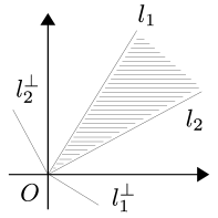
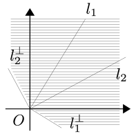
Figure 3: The left and right figures are a cone of $\mathbb{R}^{2}$ and its dual cone, respectively. For each $i=1,2$, the rays $l_{i}$ and $l_{i}^{\bot}$ are orthogonal to each other at the origin $O$.

Next, we describe a GPT, which requires the following components. Suppose that $\mathcal{K}\subset\mathcal{V}$ is a proper cone, i.e., a cone satisfying $\operatorname{int}(\mathcal{K})\not=\emptyset$ and $\mathcal{K}\cap(-\mathcal{K})=\{0\}$, where $\operatorname{int}(\mathcal{X})$ denotes the interior of a subset $\mathcal{X}\subset\mathcal{V}$. Once we fix a unit effect $u\in\operatorname{int}(\mathcal{K}^{\ast})$, the set of all states is given as

$$\mathcal{S}(\mathcal{K},u)\coloneqq\set{x\in\mathcal{K}}{\braket{u,x}=1}.$$

The set $\mathcal{S}(\mathcal{K},u)$ is a compact convex set (see Lemma C.6 in Appendix C). A measurement is given as a decomposition $\{e_{i}\}_{i}$ of $u$, namely, it satisfies $e_{i}\in\mathcal{K}^{\ast}$ and $\sum_{i}e_{i}=u$, where each $i$ corresponds to an outcome. When $x$ is a state and a measurement $\{e_{i}\}_{i}$ is performed, the probability to obtain an outcome $i$ is $\braket{e_{i},x}$. Therefore, once we fix the tuple $(\mathcal{V},\braket{\cdot,\cdot},\mathcal{K},u)$, our GPT is established.

Next, we give two typical examples of GPTs. Table 1 summarizes the tuples $(\mathcal{V},\braket{\cdot,\cdot},\mathcal{K},u)$ which appear below.

Example 3.1 (Classical probability theory).

In order to recover classical probability theory with $d$ outcomes, put $\mathcal{V}=\mathbb{R}^{d}$ and $\mathcal{K}=[0,\infty)^{d}$. Also, choose the inner product $\braket{\cdot,\cdot}$ to be the standard inner product. Hence the relation $\mathcal{K}^{\ast}=[0,\infty)^{d}$ holds, and thus $\mathcal{K}$ is self-dual. Furthermore, choosing the unit effect $u=[1,\ldots,1]^{\top}$, we find that states equal probability vectors. Thus we obtain classical probability theory with $d$ outcomes.

Example 3.2 (Quantum theory).

Next, let us recover quantum theory on a finite-dimensional complex Hilbert space $\mathcal{H}$. Choose $\mathcal{V}$ to be the set $\mathcal{T}(\mathcal{H})$ of all Hermitian matrices on $\mathcal{H}$. Also, choose $\mathcal{K}$ to be the set $\mathcal{T}_{+}(\mathcal{H})$ of all positive semi-definite matrices, which has non-empty interior and satisfies $\mathcal{T}_{+}(\mathcal{H})\cap(-\mathcal{T}_{+}(\mathcal{H}))=\{0\}$. Furthermore, define the inner product $\braket{\cdot,\cdot}$ as $\braket{Y,X}=\Tr YX$ for all $X,Y\in\mathcal{T}(\mathcal{H})$. Hence the relation $\mathcal{K}^{\ast}=\mathcal{T}_{+}(\mathcal{H})$ holds, and thus $\mathcal{K}$ is self-dual. Choosing the unit effect $u$ to be the identity matrix on $\mathcal{H}$, we find that states equal density matrices. Finally, we note that measurements are given as positive operator-valued measures (POVMs).

Table 1: The two tuples $(\mathcal{V},\braket{\cdot,\cdot},\mathcal{K},u)$ in Examples 3.1 and 3.2.

	Vector space $\mathcal{V}$	Inner product $\braket{\cdot,\cdot}$
Classical	$\mathbb{R}^{d}$	$\sum_{i=1}^{d}y_{i}x_{i}$
Quantum	All Hermitian matrices	$\Tr YX$
	Proper cone $\mathcal{K}$	Unit effect $u$
Classical	$[0,\infty)^{d}$	$[1,\ldots,1]^{\top}$
Quantum	All positive semi-definite matrices	Identity matrix

Now, we return to GPTs and focus on two GPTs given by two tuples $(\mathcal{V}_{i},\braket{\cdot,\cdot},\mathcal{K}_{i},u_{i})$ with $i=1,2$. The joint system is given as the tensor product space $\mathcal{V}_{1}\otimes\mathcal{V}_{2}$ equipped with the natural inner product induced by the inner products of $\mathcal{V}_{1}$ and $\mathcal{V}_{2}$. Then the joint unit effect is $u_{1}\otimes u_{2}$. When two states $x_{1}\in\mathcal{S}(\mathcal{K}_{1},u_{1})$ and $x_{2}\in\mathcal{S}(\mathcal{K}_{2},u_{2})$ are prepared independently in the respective systems, it is natural that the state on the joint system is given as the product state $x_{1}\otimes x_{2}$. Since any convex combination of product states is also realized by randomization, any state $x\in\mathcal{S}(\mathcal{K}_{1}\otimes\mathcal{K}_{2},u_{1}\otimes u_{2})$ can be realized. Here we define the tensor product cone $\mathcal{K}_{1}\otimes\mathcal{K}_{2}$ as

$$\mathcal{K}_{1}\otimes\mathcal{K}_{2}=\Set{\sum_{i=1}^{n}x_{i,1}\otimes x_{i,2}\in\mathcal{V}_{1}\otimes\mathcal{V}_{2}}{n\in\mathbb{N},\ x_{i,1}\in\mathcal{K}_{1},\ x_{i,2}\in\mathcal{K}_{2}\ (1\leq i\leq n)}.$$

Moreover, any $\sum_{i=1}^{m}x_{i,1}\otimes x_{i,2}\in\mathcal{K}_{1}\otimes\mathcal{K}_{2}$ and any $\sum_{j=1}^{n}y_{j,1}\otimes y_{j,2}\in\mathcal{K}_{1}^{\ast}\otimes\mathcal{K}_{2}^{\ast}$ satisfy

$$\Bigl{\langle}\sum_{i=1}^{m}x_{i,1}\otimes x_{i,2},\ \sum_{j=1}^{n}y_{j,1}\otimes y_{j,2}\Bigr{\rangle}=\sum_{i=1}^{m}\sum_{j=1}^{n}\braket{x_{i,1},y_{j,1}}\braket{x_{i,2},y_{j,2}}\geq 0.$$

Thus the following proposition holds:

Proposition 3.3.

If $\mathcal{K}_{1}$ and $\mathcal{K}_{2}$ are cones, then

$$\mathcal{K}_{1}^{\ast}\otimes\mathcal{K}_{2}^{\ast}\subset(\mathcal{K}_{1}\otimes\mathcal{K}_{2})^{\ast}.$$

Finally, we consider what properties a cone $\tilde{\mathcal{K}}$ of the joint system should satisfy. From the argument in the previous paragraph, the cone $\tilde{\mathcal{K}}$ must contain $\mathcal{K}_{1}\otimes\mathcal{K}_{2}$. Similarly, by considering that two measurements are performed independently in the respective systems, we obtain $\mathcal{K}_{1}^{\ast}\otimes\mathcal{K}_{2}^{\ast}\subset\tilde{\mathcal{K}}^{\ast}$. Hence $\tilde{\mathcal{K}}$ must satisfy

$$\tilde{\mathcal{K}}_{\min}\coloneqq\mathcal{K}_{1}\otimes\mathcal{K}_{2}\subset\tilde{\mathcal{K}}\subset(\mathcal{K}_{1}^{\ast}\otimes\mathcal{K}_{2}^{\ast})^{\ast}\eqqcolon\tilde{\mathcal{K}}_{\max},$$

where we note that the relation $\tilde{\mathcal{K}}_{\min}\subset\tilde{\mathcal{K}}_{\max}$ holds due to Proposition 3.3. Of course, the cone $\tilde{\mathcal{K}}$ is not necessarily unique, since $\tilde{\mathcal{K}}_{\min}\not=\tilde{\mathcal{K}}_{\max}$ in general. In fact, even if both $\mathcal{K}_{1}$ and $\mathcal{K}_{2}$ are self-dual, the cone $\tilde{\mathcal{K}}_{\min}$ is not necessarily self-dual. To see this fact, we discuss two quantum systems as follows:

Example 3.4.

We consider quantum theory on finite-dimensional complex Hilbert spaces $\mathcal{H}_{1}$ and $\mathcal{H}_{2}$. Then the vector spaces of the first, second, and joint systems are $\mathcal{T}(\mathcal{H}_{1})$, $\mathcal{T}(\mathcal{H}_{2})$, and $\mathcal{T}(\mathcal{H}_{1}\otimes\mathcal{H}_{2})$, respectively. States on the joint system are density matrices in $\mathcal{T}_{+}(\mathcal{H}_{1}\otimes\mathcal{H}_{2})$. Let $\ket{a_{i}},\ket{b_{i}}\in\mathcal{H}_{i}$ be orthonormal vectors for each $i=1,2$. When defining the unit vector $\ket{\Phi}=(\ket{a_{1}}\ket{a_{2}}+\ket{b_{1}}\ket{b_{2}})/\sqrt{2}\in\mathcal{H}_{1}\otimes\mathcal{H}_{2}$, it is well-known that the state $\ket{\Phi}\!\bra{\Phi}$ on the joint system is not separable [6, Section 1.4], i.e.,

$$\ket{\Phi}\!\bra{\Phi}\not\in\operatorname{Sep}(\mathcal{H}_{1};\mathcal{H}_{2})\coloneqq\mathcal{T}_{+}(\mathcal{H}_{1})\otimes\mathcal{T}_{+}(\mathcal{H}_{2}).$$

Thus the cone $\mathcal{T}_{+}(\mathcal{H}_{1}\otimes\mathcal{H}_{2})$ strictly contains $\operatorname{Sep}(\mathcal{H}_{1};\mathcal{H}_{2})$. Noting the inclusion relation

$$\operatorname{Sep}(\mathcal{H}_{1};\mathcal{H}_{2})\subset\mathcal{T}_{+}(\mathcal{H}_{1}\otimes\mathcal{H}_{2})\subset\operatorname{Sep}(\mathcal{H}_{1};\mathcal{H}_{2})^{\ast},$$

we obtain $\operatorname{Sep}(\mathcal{H}_{1};\mathcal{H}_{2})\not=\operatorname{Sep}(\mathcal{H}_{1};\mathcal{H}_{2})^{\ast}$. Therefore, the cones $\mathcal{T}_{+}(\mathcal{H}_{1})$ and $\mathcal{T}_{+}(\mathcal{H}_{2})$ are self-dual, but $\operatorname{Sep}(\mathcal{H}_{1};\mathcal{H}_{2})$ is not self-dual.

4 $\mathcal{K}$-positive maps and $(\mathcal{K},u)$-dynamical maps

In order to address Markovian dynamics, we describe dynamical maps. Suppose that two tuples $(\mathcal{V},\braket{\cdot,\cdot},\mathcal{K},u)$ and $(\mathcal{V}^{\prime},\braket{\cdot,\cdot},\mathcal{K}^{\prime},u^{\prime})$ give GPTs. Since a dynamical map $A$ transmits states $x\in\mathcal{S}(\mathcal{K},u)$ to states $Ax\in\mathcal{S}(\mathcal{K}^{\prime},u^{\prime})$, a dynamical map must satisfy some properties. First, a dynamical map $A$ is a linear map from $\mathcal{V}$ into $\mathcal{V}^{\prime}$ because $A$ needs to preserve the convex combination structure. Moreover, the linear map $A$ must satisfy the following properties:

Definition 4.1 ($(\mathcal{K};\mathcal{K}^{\prime})$-positivity).

If a linear map $A:\mathcal{V}\to\mathcal{V}^{\prime}$ satisfies $A\mathcal{K}\subset\mathcal{K}^{\prime}$, we say that $A$ is $(\mathcal{K};\mathcal{K}^{\prime})$-positive.

Definition 4.2 (Dual $(u;u^{\prime})$-preserving).

If a linear map $A:\mathcal{V}\to\mathcal{V}^{\prime}$ satisfies $A^{\ast}u^{\prime}=u$, we say that $A$ is dual $(u;u^{\prime})$-preserving, where $A^{\ast}$ denotes the adjoint map of $A$.

If a linear map $A$ is $(\mathcal{K};\mathcal{K}^{\prime})$-positive and dual $(u;u^{\prime})$-preserving, we say that $A$ is $(\mathcal{K},u;\mathcal{K}^{\prime},u^{\prime})$-dynamical. A linear map $A$ is $(\mathcal{K},u;\mathcal{K}^{\prime},u^{\prime})$-dynamical if and only if the inclusion relation $A\mathcal{S}(\mathcal{K},u)\subset\mathcal{S}(\mathcal{K}^{\prime},u^{\prime})$ holds. In this paper, we consider the case $(\mathcal{V},\braket{\cdot,\cdot},\mathcal{K},u)=(\mathcal{V}^{\prime},\braket{\cdot,\cdot},\mathcal{K}^{\prime},u^{\prime})$ unless otherwise noted. In this case, the above properties are called $\mathcal{K}$-positivity, dual $u$-preserving, and $(\mathcal{K},u)$-dynamical property, respectively. Unless there is confusion, a $(\mathcal{K},u)$-dynamical map is called a dynamical map simply.

The definition of dynamical maps is different from that of quantum channels. In quantum theory, quantum channels are given as TP-CP maps. Trace-preserving and positivity in quantum theory correspond to dual $u$-preserving and $\mathcal{K}$-positivity, respectively. Hence a $(\mathcal{K},u)$-dynamical map is a counterpart of a trace-preserving and positive map in quantum theory. Moreover, our class is strictly lager than the class of TP-CP maps. The correspondences are summarized in Table 2.

Table 2: Properties for linear maps in quantum theory and GPTs.

Quantum theory	GPTs
Positivity	$\mathcal{K}$-positivity
Trace-preserving (TP)	Dual $u$-preserving
Complete positivity (CP)
TP and positivity	$(\mathcal{K},u)$-dynamical property

As stated in Section 1, to handle stochastic operation including SLOCC, we need to address dynamical maps without dual $u$-preserving. Fortunately, most results in this paper do not require dual $u$-preserving. Hence we focus on $\mathcal{K}$-positive maps mainly. As known in preceding studies [30, 29], $\mathcal{K}$-positivity guarantees a few good properties. Before stating them, we introduce several basic terms in linear algebra below.

For a linear map $A$ and its eigenvalue $\lambda$, the multiplicity as a root of the characteristic polynomial is called the algebraic multiplicity and denoted by $\operatorname{am}(A;\lambda)$. Also, the dimension of the eigenspace $\mathcal{W}(A;\lambda)\coloneqq\operatorname{Ker}(A-\lambda\operatorname{id}_{\mathcal{V}})$ is called the geometric multiplicity and denoted by $\operatorname{gm}(A;\lambda)$. For convenience, we define $\operatorname{am}(A;\lambda)=\operatorname{gm}(A;\lambda)=0$ if $\lambda$ is not an eigenvalue of $A$. For any linear map $A$ and any $\lambda\in\mathbb{C}$, the inequality $\operatorname{gm}(A;\lambda)\leq\operatorname{am}(A;\lambda)$ holds. As another basic term, the greatest absolute value of all eigenvalues of a linear map $A$ is called the spectral radius and denoted by $r(A)$ [31]. The spectral radius satisfies

$$r(A)=\limsup_{n\to\infty}\|A^{n}\|^{1/n},$$

where $\|A\|$ is the operator norm of $A$ based on the norm on $\mathcal{V}$. Since two arbitrary norms on a finite-dimensional vector space are uniformly equivalent to each other, we can select any norm instead of that above. Moreover, the equations $r(A_{1}\otimes A_{2})=r(A_{1})r(A_{2})$ and $r(A^{\ast})=r(A)$ hold. For details, see [31].

In addition to the above terms, we also define the degree of an eigenvalue of a linear map:

Definition 4.3 (Degree of eigenvalues [29, Definition 3.1]).

For a linear map $A$ and its eigenvalue $\lambda$, the degree of $\lambda$ is defined as the size of the largest Jordan block associated with $\lambda$, in the Jordan canonical form of $A$.

For instance, the matrix

$$\begin{bmatrix}0\\ &0&1\\ &0&0\\ &&&1\\ &&&&1\end{bmatrix},$$

which is already a Jordan canonical form, has the eigenvalues $0$ and $1$. In this case, the degrees of $0$ and $1$ are two and one, respectively. Now, we have been ready to state the following proposition [29, Theorem 3.1]:

Proposition 4.4.

If $A$ is a $\mathcal{K}$-positive map, then the following properties hold.

• $r(A)$ is an eigenvalue of $A$.

• $\mathcal{K}$ contains an eigenvector of $A$ associated with $r(A)$.

• The degree of $r(A)$ is greater than or equal to the degree of any other eigenvalue whose absolute value is $r(A)$.

If $\operatorname{am}(A;r(A))=1$, then the Jordan block associated with $r(A)$ is the matrix $[r(A)]$ alone, and thus the degree of $r(A)$ is one. In this case, Proposition 4.4 implies that any Jordan block associated with any eigenvalue $\lambda$ satisfying $|\lambda|=r(A)$ equals the matrix $[\lambda]$. In other words, $\operatorname{am}(A;\lambda)=\operatorname{gm}(A;\lambda)$ for any eigenvalue $\lambda$ satisfying $|\lambda|=r(A)$. We summarize the above argument as the following corollary:

Corollary 4.5.

If $A$ is a $\mathcal{K}$-positive map and satisfies $\operatorname{am}(A;r(A))=1$, then $\operatorname{am}(A;\lambda)=\operatorname{gm}(A;\lambda)$ for any eigenvalue $\lambda$ whose absolute value is $r(A)$.

Finally, we show the following basic propositions.

Proposition 4.6.

If a linear map $A$ is $\mathcal{K}$-positive, then $A^{\ast}$ is $\mathcal{K}^{\ast}$-positive.

Proof.

Let $y\in\mathcal{K}^{\ast}$. Any $x\in\mathcal{K}$ satisfies $\braket{A^{\ast}y,x}=\braket{y,Ax}\geq 0$, whence $A^{\ast}y\in\mathcal{K}^{\ast}$. ∎

Proposition 4.7.

Any dynamical map $A$ satisfies $r(A)=1$.

Proof.

Proposition 4.4 implies that $A$ has an eigenvector $x_{0}\in\mathcal{K}$ associated with $r(A)$. Since $A^{\ast}u=u$ and $u\in\operatorname{int}(\mathcal{K}^{\ast})$, we have $\braket{u,x_{0}}=\braket{A^{\ast}u,x_{0}}=\braket{u,Ax_{0}}=r(A)\braket{u,x_{0}}$ and $\braket{u,x_{0}}>0$ because of Lemma C.1 in Appendix C. Therefore, $r(A)=1$. ∎

5 Asymptotic properties for Markovian dynamics

In this section, we address asymptotic properties for Markovian dynamics in GPTs. Sections 5.1–5.3 is the discrete case, and Section 5.4 is the continuous case. Theorems 2.3, 2.4, and 2.7 are derived from Theorems 5.3, 5.4, and 5.20, respectively. Also, Theorems 2.10, 2.11, and 2.12 are derived from Theorems 5.23, 5.24, and 5.26, respectively. Throughout this section, suppose that a tuple $(\mathcal{V}_{i},\braket{\cdot,\cdot},\mathcal{K}_{i},u_{i})$ gives a GPT for each $i=1,2$. Also, suppose that a tuple $(\mathcal{V}_{1}\otimes\mathcal{V}_{2},\braket{\cdot,\cdot},\tilde{\mathcal{K}},u_{1}\otimes u_{2})$ gives a GPT on the joint system, where $\tilde{\mathcal{K}}_{\min}\subset\tilde{\mathcal{K}}\subset\tilde{\mathcal{K}}_{\max}$. We use tilde to express to be bipartite in the same way as Section 2.

5.1 Asymptotic decoupling

First, to define asymptotic decoupling in the framework of GPTs, for a state $\tilde{x}$ on the joint system, we must define the reduced state $\pi_{i}\tilde{x}$ on the $i$-th system. The reduced state $\pi_{i}\tilde{x}$ represents the state from a viewpoint of an observer of the $i$-th system. In our context, it is convenient to define the reduced states $\pi_{1}\tilde{x}$ and $\pi_{2}\tilde{x}$ for a state $\tilde{x}\in\mathcal{S}(\tilde{\mathcal{K}}_{\max},u_{1}\otimes u_{2})$ because the cone $\tilde{\mathcal{K}}_{\max}$ is largest of all cones $\tilde{\mathcal{K}}$ of the joint system. The reduced state $\pi_{1}(\tilde{x};u_{1},u_{2})$ of $\tilde{x}\in\mathcal{S}(\tilde{\mathcal{K}}_{\max},u_{1}\otimes u_{2})$ is defined by the condition

$$\forall y_{1}\in\mathcal{K}_{1}^{\ast},\quad\braket{y_{1},\pi_{1}(\tilde{x};u_{1},u_{2})}=\braket{y_{1}\otimes u_{2},\tilde{x}}.$$ (3)

Since $\mathcal{K}_{1}^{\ast}$ has non-empty interior, the Riesz representation theorem guarantees the unique existence of $\pi_{1}(\tilde{x};u_{1},u_{2})\in\mathcal{V}_{1}$. Let us verify $\pi_{1}(\tilde{x};u_{1},u_{2})\in\mathcal{S}(\mathcal{K}_{1},u_{1})$ as follows. Since $\tilde{x}\in\mathcal{S}(\tilde{\mathcal{K}}_{\max},u_{1}\otimes u_{2})$, the right-hand side of (3) is greater than or equal to zero, which implies $\pi_{1}(\tilde{x};u_{1},u_{2})\in\mathcal{K}_{1}$. Moreover, putting $y_{1}=u_{1}$ in (3), we find that

$$\braket{u_{1},\pi_{1}(\tilde{x};u_{1},u_{2})}=\braket{u_{1}\otimes u_{2},\tilde{x}}=1.$$

Therefore, $\pi_{1}(\tilde{x};u_{1},u_{2})\in\mathcal{S}(\mathcal{K}_{1},u_{1})$. The reduced state $\pi_{2}(\tilde{x};u_{1},u_{2})\in\mathcal{S}(\mathcal{K}_{2},u_{2})$ is also defined similarly. Unless there is confusion, we express $\pi_{i}(\tilde{x};u_{1},u_{2})$ as $\pi_{i}\tilde{x}$ simply. Then $\pi_{i}$ can be naturally regarded as a linear map from $\mathcal{V}_{1}\otimes\mathcal{V}_{2}$ onto $\mathcal{V}_{i}$.

Next, to define asymptotic decoupling for (not necessarily $\tilde{\mathcal{K}}$-positive) linear maps, we introduce the set

$$\mathcal{D}_{n}(\tilde{A})\coloneqq\Set{\tilde{x}\in\tilde{\mathcal{K}}\setminus\{0\}}{\tilde{A}^{k}\tilde{x}\in\tilde{\mathcal{K}}_{\max}\setminus\{0\}\ (\forall k\geq n)}$$

for a linear map $\tilde{A}$ and $n\in\mathbb{N}$. Then the monotonicity $\mathcal{D}_{1}(\tilde{A})\subset\mathcal{D}_{2}(\tilde{A})\subset\cdots$ holds. By using the sets $\mathcal{D}_{n}(\tilde{A})$, asymptotic decoupling is defined as follows:

Definition 5.1 ($(\tilde{\mathcal{K}},u_{1},u_{2})$-asymptotic decoupling).

Suppose that a dual $u_{1}\otimes u_{2}$-preserving map $\tilde{A}$ satisfies

$$\bigcup_{n=1}^{\infty}\mathcal{D}_{n}(\tilde{A})=\tilde{\mathcal{K}}\setminus\{0\}.$$ (4)

Then $\tilde{A}$ is $(\tilde{\mathcal{K}},u_{1},u_{2})$-asymptotically decoupling if any state $\tilde{x}\in\mathcal{S}(\tilde{\mathcal{K}},u_{1}\otimes u_{2})$ satisfies

$$\tilde{A}^{n}\tilde{x}=\pi_{1}\tilde{A}^{n}\tilde{x}\otimes\pi_{2}\tilde{A}^{n}\tilde{x}+o(1)\quad(n\to\infty).$$ (5)

The assumption (4) allows us to consider the limit (5). Definition 5.1 needs (4), but one may not mind (4) because for any two dynamical maps $A_{1}$ and $A_{2}$, the tensor product map $\tilde{A}=A_{1}\otimes A_{2}$ satisfies (4) (see Lemma A.1 in Appendix A). In this case, we can simplify (5):

$$(A_{1}\otimes A_{2})^{n}(\tilde{x}-\pi_{1}\tilde{x}\otimes\pi_{2}\tilde{x})=o(1).$$

Next, to clarify a necessary and sufficient condition of asymptotic decoupling, we introduce another asymptotic property, namely, mixing:

Definition 5.2 (Mixing).

A dynamical map $A$ is mixing if there exists a state $x_{0}\in\mathcal{S}(\mathcal{K},u)$ such that any state $x\in\mathcal{S}(\mathcal{K},u)$ satisfies

$$\lim_{n\to\infty}A^{n}x=x_{0}.$$

The state $x_{0}$ is called the stationary state.

In the same way as Section 2, we give a necessary and sufficient condition of asymptotic decoupling for a tensor product map $A_{1}\otimes A_{2}$ and a linear map $\tilde{A}$ in this order:

Theorem 5.3.

For any two dynamical maps $A_{1}$ and $A_{2}$, the following conditions are equivalent.

1. $A_{1}\otimes A_{2}$ is $(\tilde{\mathcal{K}},u_{1},u_{2})$-asymptotically decoupling.

2. $A_{1}$ or $A_{2}$ at least one is mixing.

Theorem 5.4.

For any dual $u_{1}\otimes u_{2}$-preserving map $\tilde{A}$ with (4), the following conditions are equivalent.

1. $\tilde{A}$ is $(\tilde{\mathcal{K}},u_{1},u_{2})$-asymptotically decoupling.

2. There exist a number $i_{1}\in\{1,2\}$ and a state $x_{0,i_{1}}\in\mathcal{S}(\mathcal{K}_{i_{1}},u_{i_{1}})$ such that any state $\tilde{x}\in\mathcal{S}(\tilde{\mathcal{K}},u_{1}\otimes u_{2})$ satisfies

   $$\tilde{A}^{n}\tilde{x}=x_{0,i_{1}}\otimes\pi_{i_{2}}\tilde{A}^{n}\tilde{x}+o(1)\quad(n\to\infty),$$

   where $i_{2}$ is an element of $\{1,2\}$ except for $i_{1}$.

Since Theorem 5.3 follows from Theorem 5.4 immediately, all we need is to show Theorem 5.4. To show Theorem 5.4, we introduce a non-asymptotic property on the joint system, namely, decoupling:

Definition 5.5 ($(\tilde{\mathcal{K}},u_{1},u_{2})$-decoupling).

Suppose that a dual $u_{1}\otimes u_{2}$-preserving map $\tilde{A}$ satisfies

$$\tilde{A}(\tilde{\mathcal{K}}\setminus\{0\})\subset\tilde{\mathcal{K}}_{\max}\setminus\{0\}.$$ (6)

Then $\tilde{A}$ is decoupling if any state $\tilde{x}\in\mathcal{S}(\tilde{\mathcal{K}},u_{1}\otimes u_{2})$ satisfies

$$\tilde{A}\tilde{x}=\pi_{1}\tilde{A}\tilde{x}\otimes\pi_{2}\tilde{A}\tilde{x}.$$

Decoupling asserts that $\tilde{A}$ breaks the correlation between two systems completely. To prove Theorem 5.4, we give a necessary and sufficient condition of decoupling, which can be regarded as the non-asymptotic version of Theorem 5.3.

Lemma 5.6.

For any dual $u_{1}\otimes u_{2}$-preserving map $\tilde{A}$ with (6), the following conditions are equivalent.

1. $\tilde{A}$ is $(\tilde{\mathcal{K}},u_{1},u_{2})$-decoupling.

2. There exist a number $i_{1}\in\{1,2\}$ and a state $x_{0,i_{1}}\in\mathcal{S}(\mathcal{K}_{i_{1}},u_{i_{1}})$ such that any state $\tilde{x}\in\mathcal{S}(\tilde{\mathcal{K}},u_{1}\otimes u_{2})$ satisfies

   $$\tilde{A}\tilde{x}=x_{0,i_{1}}\otimes\pi_{i_{2}}\tilde{A}\tilde{x},$$

   where $i_{2}$ is an element of $\{1,2\}$ except for $i_{1}$.

Proof.

(2)$\Rightarrow$(1). This implication follows from the definition.

(1)$\Rightarrow$(2). Assume condition (1). Then condition (2) follows from the following steps.

Step 1. First, we show that any two states $\tilde{x},\tilde{x}^{\prime}\in\mathcal{S}(\tilde{\mathcal{K}},u_{1}\otimes u_{2})$ satisfy $\pi_{1}\tilde{A}\tilde{x}=\pi_{1}\tilde{A}\tilde{x}^{\prime}$ or $\pi_{2}\tilde{A}\tilde{x}=\pi_{2}\tilde{A}\tilde{x}^{\prime}$ at least one. Let $\tilde{x},\tilde{x}^{\prime}\in\mathcal{S}(\tilde{\mathcal{K}},u_{1}\otimes u_{2})$. Then the $(a)$ linearity and $(b)$ decoupling of $\tilde{A}$ yield

$$\frac{1}{2}\pi_{1}\tilde{A}\tilde{x}\otimes\pi_{2}\tilde{A}\tilde{x}+\frac{1}{2}\pi_{1}\tilde{A}\tilde{x}^{\prime}\otimes\pi_{2}\tilde{A}\tilde{x}^{\prime}$$

$$\overset{(b)}{=} \frac{1}{2}\tilde{A}\tilde{x}+\frac{1}{2}\tilde{A}\tilde{x}^{\prime}\overset{(a)}{=}\tilde{A}\Bigl{(}\frac{1}{2}\tilde{x}+\frac{1}{2}\tilde{x}^{\prime}\Bigr{)}$$

$$\overset{(b)}{=} \pi_{1}\tilde{A}\Bigl{(}\frac{1}{2}\tilde{x}+\frac{1}{2}\tilde{x}^{\prime}\Bigr{)}\otimes\pi_{2}\tilde{A}\Bigl{(}\frac{1}{2}\tilde{x}+\frac{1}{2}\tilde{x}^{\prime}\Bigr{)}$$

$$\overset{(a)}{=} \frac{1}{4}\pi_{1}\tilde{A}\tilde{x}\otimes\pi_{2}\tilde{A}\tilde{x}+\frac{1}{4}\pi_{1}\tilde{A}\tilde{x}^{\prime}\otimes\pi_{2}\tilde{A}\tilde{x}^{\prime}$$

$$+\frac{1}{4}\pi_{1}\tilde{A}\tilde{x}\otimes\pi_{2}\tilde{A}\tilde{x}^{\prime}+\frac{1}{4}\pi_{1}\tilde{A}\tilde{x}^{\prime}\otimes\pi_{2}\tilde{A}\tilde{x}.$$

Calculating the above both sides, we obtain

$$(\pi_{1}\tilde{A}\tilde{x}-\pi_{1}\tilde{A}\tilde{x}^{\prime})\otimes(\pi_{2}\tilde{A}\tilde{x}-\pi_{2}\tilde{A}\tilde{x}^{\prime})=0.$$

Therefore, any two states $\tilde{x},\tilde{x}^{\prime}\in\mathcal{S}(\tilde{\mathcal{K}},u_{1}\otimes u_{2})$ satisfy $\pi_{1}\tilde{A}\tilde{x}=\pi_{1}\tilde{A}\tilde{x}^{\prime}$ or $\pi_{2}\tilde{A}\tilde{x}=\pi_{2}\tilde{A}\tilde{x}^{\prime}$ at least one.

Step 2. Next, we show that there exists a number $i\in\{1,2\}$ such that any state $\tilde{x}$ satisfies $\pi_{i}\tilde{A}\tilde{x}=\pi_{i}\tilde{A}\tilde{x}^{\prime}$ by contradiction. Suppose that there existed two pairs $(\tilde{x}_{1},\tilde{x}^{\prime}_{1})$ and $(\tilde{x}_{2},\tilde{x}^{\prime}_{2})$ of two states such that

$$\pi_{1}\tilde{A}\tilde{x}_{1}\not=\pi_{1}\tilde{A}\tilde{x}^{\prime}_{1},\quad\pi_{2}\tilde{A}\tilde{x}_{2}\not=\pi_{2}\tilde{A}\tilde{x}^{\prime}_{2}.$$ (7)

Then step 1 implies

$$\pi_{2}\tilde{A}\tilde{x}_{1}=\pi_{2}\tilde{A}\tilde{x}^{\prime}_{1},\quad\pi_{1}\tilde{A}\tilde{x}_{2}=\pi_{1}\tilde{A}\tilde{x}^{\prime}_{2}.$$

Also, thanks to the pigeonhole principle, there exists a number $i_{0}\in\{1,2\}$ such that two of the following three cases hold:

1. $\pi_{i_{0}}\tilde{A}(\tilde{x}_{1}+\tilde{x}^{\prime}_{1})/2=\pi_{i_{0}}\tilde{A}(\tilde{x}_{2}+\tilde{x}^{\prime}_{2})/2$,

2. $\pi_{i_{0}}\tilde{A}(\tilde{x}_{1}+\tilde{x}_{2})/2=\pi_{i_{0}}\tilde{A}(\tilde{x}^{\prime}_{1}+\tilde{x}^{\prime}_{2})/2$,

3. $\pi_{i_{0}}\tilde{A}(\tilde{x}_{1}+\tilde{x}^{\prime}_{2})/2=\pi_{i_{0}}\tilde{A}(\tilde{x}^{\prime}_{1}+\tilde{x}_{2})/2$.

For instance, suppose that cases (i) and (ii) (which we call {(i),(ii)} case) hold. Taking the sum of cases (i) and (ii), we obtain $\pi_{i_{0}}\tilde{A}\tilde{x}_{1}=\pi_{i_{0}}\tilde{A}\tilde{x}^{\prime}_{2}$. This equation and case (i) yield $\pi_{i_{0}}\tilde{A}\tilde{x}^{\prime}_{1}=\pi_{i_{0}}\tilde{A}\tilde{x}_{2}$. However, if $i_{0}=1$, it follows that

$$\pi_{1}\tilde{A}\tilde{x}_{1}=\pi_{1}\tilde{A}\tilde{x}^{\prime}_{2}=\pi_{1}\tilde{A}\tilde{x}_{2}=\pi_{1}\tilde{A}\tilde{x}^{\prime}_{1},$$

which contradicts (7). Similarly, if $i_{0}=2$, it follows that

$$\pi_{2}\tilde{A}\tilde{x}_{2}=\pi_{2}\tilde{A}\tilde{x}^{\prime}_{1}=\pi_{2}\tilde{A}\tilde{x}_{1}=\pi_{2}\tilde{A}\tilde{x}^{\prime}_{2},$$

which contradicts (7). The other cases, namely, {(i),(iii)} and {(ii),(iii)} cases also have contradictions in the same way. Therefore, there exists a number $i\in\{1,2\}$ such that any two states $\tilde{x},\tilde{x}^{\prime}\in\mathcal{S}(\tilde{\mathcal{K}},u_{1}\otimes u_{2})$ satisfy $\pi_{i}\tilde{A}\tilde{x}=\pi_{i}\tilde{A}\tilde{x}^{\prime}$.

Step 3. Step 2 implies that $\pi_{i}\tilde{A}\tilde{x}$ does not depend on $\tilde{x}\in\mathcal{S}(\tilde{\mathcal{K}},u_{1}\otimes u_{2})$. That is, there exists a state $x_{0,i}\in\mathcal{S}(\mathcal{K}_{i},u_{i})$ such that any state $\tilde{x}\in\mathcal{S}(\tilde{\mathcal{K}},u_{1}\otimes u_{2})$ satisfies $\pi_{i}\tilde{A}\tilde{x}=x_{0,i}$. Thus this equation and condition (1) yield condition (2). ∎

Moreover, to prove Theorem 5.4, we need the following technical lemmas:

Lemma 5.7 (Compactness).

The set of all $(\mathcal{K},u;\mathcal{K}^{\prime},u^{\prime})$-dynamical maps is compact.

Lemma 5.8 (Invariance of ranges).

Let $A$ be a dynamical map. If $A_{0}$ and $A^{\prime}_{0}$ are the limits of two convergent subsequences $\{A^{n}\}_{n\in N\subset\mathbb{N}}$ and $\{A^{n}\}_{n\in N^{\prime}\subset\mathbb{N}}$, respectively, then $\operatorname{Ran}A_{0}=\operatorname{Ran}A^{\prime}_{0}$.

Lemmas 5.7 and 5.8 are proved in Appendix A.

Proof of Theorem 5.4.

(2)$\Rightarrow$(1). This implication follows from the definition.

(1)$\Rightarrow$(2). Assume condition (1). Then condition (2) follows from the following steps.

Step 1. First, we show that there exist a number $i_{1}\in\{1,2\}$ and a state $x_{0,i_{1}}\in\mathcal{S}(\mathcal{K}_{i_{1}},u_{i_{1}})$ such that the limit $\tilde{A}_{0}$ of any convergent subsequence of $\{\tilde{A}^{n}\}_{n\in\mathbb{N}}$ satisfies

$$\tilde{A}_{0}(\cdot)=x_{0,i_{1}}\otimes\pi_{i_{2}}\tilde{A}_{0}(\cdot),$$

where $i_{2}$ is an element of $\{1,2\}$ except for $i_{1}$. Take an arbitrary convergent subsequence $\{\tilde{A}^{n}\}_{n\in N\subset\mathbb{N}}$. Then the limit $\tilde{A}_{0}$ of $\{\tilde{A}^{n}\}_{n\in N}$ is decoupling. By changing the subscripts if necessary, Lemma 5.6 implies that there exists a state $x_{0,1}\in\mathcal{S}(\mathcal{K}_{1},u_{1})$ such that

$$\tilde{A}_{0}(\cdot)=x_{0,1}\otimes\pi_{2}\tilde{A}_{0}(\cdot).$$

The subscript $1$ and the state $x_{0,1}$ are independent of convergent subsequences of $\{\tilde{A}^{n}\}_{n\in\mathbb{N}}$, due to Lemma 5.8. Therefore, the assertion in this step follows.

Step 2. Next, we show that the sequence $\{\pi_{1}\tilde{A}^{n}\}_{n\in\mathbb{N}}$ converges to $\braket{u_{1}\otimes u_{2},\cdot}x_{0,1}$. Take an arbitrary convergent subsequence $\{\pi_{1}\tilde{A}^{n}\}_{n\in N\subset\mathbb{N}}$. Due to Lemma 5.7, we can take a subsequence $\{\pi_{1}\tilde{A}^{n}\}_{n\in N^{\prime}\subset N}$ such that the sequence $\{\tilde{A}^{n}\}_{n\in N^{\prime}}$ converges. Step 1 implies that the limit of $\{\pi_{1}\tilde{A}^{n}\}_{n\in N^{\prime}}$ is $\braket{u_{1}\otimes u_{2},\cdot}x_{0,1}$. Therefore, any convergent subsequence of $\{\pi_{1}\tilde{A}^{n}\}_{n\in\mathbb{N}}$ converges to $\braket{u_{1}\otimes u_{2},\cdot}x_{0,1}$. Thus Lemma 5.7 implies that the sequence $\{\pi_{1}\tilde{A}^{n}\}_{n\in\mathbb{N}}$ converges to $\braket{u_{1}\otimes u_{2},\cdot}x_{0,1}$.

Step 3. Finally, step 2 and condition (1) imply that any state $\tilde{x}\in\mathcal{S}(\tilde{\mathcal{K}},u_{1}\otimes u_{2})$ satisfies

$$\tilde{A}^{n}\tilde{x} =\pi_{1}\tilde{A}^{n}\tilde{x}\otimes\pi_{2}\tilde{A}^{n}\tilde{x}+o(1)$$

$$=x_{0,1}\otimes\pi_{2}\tilde{A}^{n}\tilde{x}+o(1),$$

which is just condition (2). ∎

So far, we have defined asymptotic decoupling for dynamical maps, and have given its necessary and sufficient condition. However, to handle stochastic operation including SLOCC, we need to address dynamical maps without dual $u_{1}\otimes u_{2}$-preserving. In the case without dual $u_{1}\otimes u_{2}$-preserving, the definitions of asymptotic decoupling and mixing are modified as follows.

Definition 5.9 ($(\tilde{\mathcal{K}},u_{1},u_{2})$-asymptotic decoupling).

A linear map $\tilde{A}$ with (4) is $(\tilde{\mathcal{K}},u_{1},u_{2})$-asymptotically decoupling if any state $\tilde{x}\in\mathcal{S}(\tilde{\mathcal{K}},u_{1}\otimes u_{2})$ satisfies

$$\frac{\tilde{A}^{n}\tilde{x}}{\braket{u_{1}\otimes u_{2},\tilde{A}^{n}\tilde{x}}}=\frac{\pi_{1}\tilde{A}^{n}\tilde{x}}{\braket{u_{1}\otimes u_{2},\tilde{A}^{n}\tilde{x}}}\otimes\frac{\pi_{2}\tilde{A}^{n}\tilde{x}}{\braket{u_{1}\otimes u_{2},\tilde{A}^{n}\tilde{x}}}+o(1)\quad(n\to\infty).$$

Definition 5.10 (Mixing).

A linear map $A$ with $r(A)>0$ is mixing if there exist nonzero $x_{0},y_{0}\in\mathcal{V}$ such that any $x\in\mathcal{V}$ satisfies

$$\lim_{n\to\infty}(r(A)^{-1}A)^{n}x=\braket{y_{0},x}x_{0}.$$

The vectors $x_{0}$ and $y_{0}$ are called a stationary vector and a dual stationary vector, respectively.

Of course, if $\tilde{A}$ is dual $u_{1}\otimes u_{2}$-preserving, Definitions 5.1 and 5.9 are equivalent to each other. If $A$ is a dynamical map, Definitions 5.2 and 5.10 are also equivalent to each other. Indeed, if a $(\mathcal{K},u)$-dynamical map $A$ is mixing in the sense of Definition 5.10, then Proposition 4.7 implies $r(A)=1$, and we can choose a stationary vector $x_{0}$ and a dual stationary vector $y_{0}$ as $x_{0}\in\mathcal{S}(\mathcal{K},u)$ and $y_{0}=u$. Therefore, Definitions 5.9 and 5.10 are extensions of Definitions 5.1 and 5.2, respectively. By using Definitions 5.9 and 5.10, Theorem 5.3 is extended as follows:

Theorem 5.11.

Suppose that the adjoint map of a $\mathcal{K}_{i}$-positive map $A_{i}$ has an eigenvector $y_{0,i}\in\operatorname{int}(\mathcal{K}_{i})$ for each $i=1,2$. Then the following conditions are equivalent.

1. $A_{1}\otimes A_{2}$ is $(\tilde{\mathcal{K}},u_{1},u_{2})$-asymptotically decoupling.

2. $A_{1}$ or $A_{2}$ at least one is mixing.

Theorem 5.11 follows from Theorem 5.3 and the next lemma. The lemma asserts that $(\tilde{\mathcal{K}},u_{1},u_{2})$-asymptotic decoupling does not depend on the unit effect $u_{1}$ or $u_{2}$.

Lemma 5.12.

Let $u^{\prime}_{i}\in\operatorname{int}(\mathcal{K}_{i}^{\ast})$ for each $i=1,2$. If a linear map $\tilde{A}$ with (4) is $(\tilde{\mathcal{K}},u_{1},u_{2})$-asymptotically decoupling, then $\tilde{A}$ is $(\tilde{\mathcal{K}},u^{\prime}_{1},u^{\prime}_{2})$-asymptotically decoupling.

Lemma 5.12 is proved in Appendix A.

Proof of Theorem 5.11.

Without loss of generality, we may show the equivalence by assuming that the eigenvector $y_{0,i}\in\operatorname{int}(\mathcal{K}_{i})$ equals the unit effect $u_{i}$ for each $i=1,2$, due to Lemma 5.12. In the case with $y_{0,i}=u_{i}$, Theorem 5.11 follows from Theorem 5.3. Therefore, the proof is completed. ∎

5.2 Ergodicity

As proved in Section 5.1, asymptotic decoupling is equivalent to local mixing. Hence it is meaningful to investigate criteria of mixing. Although spectral criterion is known as a criterion of mixing, we give another criterion in the next subsection. For this purpose, we investigate ergodicity in this subsection, which is a weaker property than mixing. In quantum theory, ergodicity is defined for quantum channels. In GPTs, however, the definition of dynamical maps on the joint system depends on the cone $\tilde{\mathcal{K}}$ of the joint system, and the cone $\tilde{\mathcal{K}}$ is not unique. For this reason, it is convenient to define ergodicity (and mixing) for linear maps in our context. Therefore, we employ the following definition:

Definition 5.13 (Ergodicity).

A linear map $A$ with $r(A)>0$ is ergodic if there exist nonzero $x_{0},y_{0}\in\mathcal{V}$ such that any $x\in\mathcal{V}$ satisfies

$$\lim_{n\to\infty}\frac{1}{n}\sum_{k=0}^{n-1}(r(A)^{-1}A)^{k}x=\braket{y_{0},x}x_{0}.$$

The vectors $x_{0}$ and $y_{0}$ are called a stationary vector and a dual stationary vector, respectively.

If $A$ is a dynamical map, Definition 5.13 can be represented like Definition 2.5. Indeed, if a $(\mathcal{K},u)$-dynamical map $A$ is ergodic, then Proposition 4.7 implies $r(A)=1$, and we can choose a stationary vector $x_{0}$ and a dual stationary vector $y_{0}$ as $x_{0}\in\mathcal{S}(\mathcal{K},u)$ and $y_{0}=u$. The above relation is similar to the relation between Definitions 5.2 and 5.10. Now, Definition 5.13 cannot be checked directly by numerical computation. Its numerical check is realized by the following technical lemma:

Proposition 5.14.

For any linear map $A$ with $r(A)>0$, the following conditions are equivalent.

1. $A$ is ergodic.

2. $\operatorname{am}(A;r(A))=1$ and $\operatorname{am}(A;\lambda)=\operatorname{gm}(A;\lambda)$ for any $\lambda\in\mathbb{C}$ whose absolute value is $r(A)$.

Proposition 5.14 is proved in Appendix A. If $A$ is $\mathcal{K}$-positive, condition (2) in Proposition 5.14 turns to a simpler condition:

Proposition 5.15.

For any $\mathcal{K}$-positive map $A$ with $r(A)>0$, the following conditions are equivalent.

1. $A$ is ergodic.

2. $\operatorname{am}(A;r(A))=1$.

Proof.

(1)$\Rightarrow$(2). This implication follows from Proposition 5.14.

(2)$\Rightarrow$(1). All we need is to show condition (2) in Proposition 5.14. Suppose that $\lambda\in\mathbb{C}$ satisfies $|\lambda|=r(A)$. If $\lambda$ is not an eigenvalue of $A$, of course, the equation $\operatorname{am}(A;\lambda)=\operatorname{gm}(A;\lambda)=0$ holds. If $\lambda$ is an eigenvalue of $A$, condition (2) and Corollary 4.5 imply that $\operatorname{am}(A;\lambda)=\operatorname{gm}(A;\lambda)$. Therefore, condition (2) in Proposition 5.14 holds. ∎

If $A$ is a dynamical map, condition (2) in Proposition 5.15 turns to a weaker condition:

Proposition 5.16.

For any dynamical map $A$, the following conditions are equivalent.

1. $A$ is ergodic.

2. $\operatorname{gm}(A;1)=1$. In other words, $\dim\operatorname{Ker}(A-\operatorname{id}_{\mathcal{V}})=1$.

Proposition 5.16 is well-known in quantum theory [10, appendix], [11, Corollary 2]. Here, to prove Proposition 5.16 we use Proposition 5.15 and [10, Lemma 5]. Applying [10, Lemma 5] to our setting, we obtain the following proposition immediately:

Proposition 5.17.

If a $(\mathcal{K},u)$-dynamical map $A$ has only one fixed point in $\mathcal{S}(\mathcal{K},u)$, then $A$ is ergodic.

Proof of Proposition 5.16.

(1)$\Rightarrow$(2). This implication follows from Proposition 5.15.

(2)$\Rightarrow$(1). Since $A$ is $(\mathcal{K},u)$-dynamical, Propositions 4.4 and 4.7 imply that $A$ has an eigenvector $x_{0}\in\mathcal{K}$ associated with $r(A)=1$. Without loss of generality, we may assume $x_{0}\in\mathcal{S}(\mathcal{K},u)$. Thanks to condition (2), the dynamical map $A$ has the only one fixed point $x_{0}$ in $\mathcal{S}(\mathcal{K},u)$. Thus Proposition 5.17 implies condition (1). ∎

Some researchers should know Propositions 5.14 and 5.15, but they seem not to be published. Proposition 5.16 should also be known because the quantum version of Proposition 5.16 is well-known, and the proof is the same as that of the quantum version. However, the above three propositions are not so trivial due to the difference among them. If we omitted the proofs of them, a large logical gap would occur, and thus we have proved the three propositions in this subsection.

5.3 Mixing

In this subsection, we give a criterion of mixing that is different from spectral criterion. Our criterion consists of the following two parts: (i) Proposition 5.16 and (ii) the equivalence between mixing for a dynamical map $A$ and ergodicity for the two-fold tensor product map $A^{\otimes 2}$. Since (i) is already known as stated in Section 5.2, (ii) is an essential and additional part. First, we begin with spectral criterion:

Proposition 5.18 (Spectral criterion).

For any linear map $A$ with $r(A)>0$, the following conditions are equivalent.

1. $A$ is mixing.

2. $\operatorname{am}(A;r(A))=1$ and $\operatorname{am}(A;\lambda)=0$ for any $\lambda\not=r(A)$ whose absolute value is $r(A)$.

Spectral criterion is well-known in quantum theory [10, Theorem 7], but the above general case seems not to be published. However, Proposition 5.18 can be proved in the same way as the quantum case, namely, by considering the Jordan canonical form of $A$. Moreover, the statement does not change in the three cases, namely, for linear maps, for $\mathcal{K}$-positive maps, and for dynamical maps. This is why we do not prove Proposition 5.18.

Next, let us give other conditions equivalent to mixing.

Theorem 5.19.

For any linear map $A$ with $r(A)>0$, the following conditions are equivalent.

1. $A$ is mixing.

2. $A^{\otimes 2}$ is mixing, and $A$ has the eigenvalue $r(A)$.

3. $A^{\otimes 2}$ is ergodic, and $A$ has the eigenvalue $r(A)$.

4. $\operatorname{gm}(A^{\otimes 2};r(A)^{2})=1$, and $A$ has the eigenvalue $r(A)$.

If $A$ is $\mathcal{K}$-positive, Proposition 4.4 guarantees that $A$ has the eigenvalue $r(A)$. Thus, in this case, conditions in Theorem 5.19 turn to simpler conditions:

Theorem 5.20.

For any $\mathcal{K}$-positive map $A$ with $r(A)>0$, the following conditions are equivalent.

1. $A$ is mixing.

2. $A^{\otimes 2}$ is mixing.

3. $A^{\otimes 2}$ is ergodic.

4. $\operatorname{gm}(A^{\otimes 2};r(A)^{2})=1$.

If $A$ is a dynamical map, Proposition 4.7 guarantees $r(A)=1$, and thus condition (4) can be represented as $\dim\operatorname{Ker}(A^{\otimes 2}-\operatorname{id}_{\mathcal{V}^{\otimes 2}})=1$. Hence Theorem 5.20 gives a criterion of mixing that is a system of linear equations. On the other hand, Proposition 5.18 requires us to solve an eigenequation. An eigenequation cannot be solved by finite steps in general, but a system of linear equations can always be solved, which is an advantage of Theorem 5.20. Of course, some criteria of mixing that does not require us to solve an eigenequation are known for special classes of quantum channels. For instance, Burgarth et al. [11, Theorems 10 and 13] proved that, for any quantum channel $\Gamma$ with a strictly positive semi-definite fixed point, $\Gamma$ is mixing if and only if $\Gamma^{k}$ is ergodic for all integers $1\leq k\leq(\dim\mathcal{H})^{2}$; a unital quantum channel $\Gamma$ is mixing if $\Gamma^{\ast}\circ\Gamma$ is ergodic.

To prove Theorem 5.19, let us show the following preliminary lemma:

Lemma 5.21.

If a linear map $A_{i}$ is mixing for each $i=1,2$, then $A_{1}\otimes A_{2}$ is also mixing.

Proof.

Without loss of generality, we may assume $r(A_{1})=r(A_{2})=1$. Then $r(A_{1}\otimes A_{2})=r(A_{1})r(A_{2})=1$. For all $i=1,2$ and $x_{i}\in\mathcal{V}_{i}$,

$$\lim_{n\to\infty}A_{i}^{n}x_{i}=\braket{y_{0,i},x_{i}}x_{0,i},$$

where $x_{0,i}$ and $y_{0,i}$ are a stationary vector and a dual stationary vector of $A_{i}$, respectively. Thus any $\tilde{x}\in\mathcal{V}_{1}\otimes\mathcal{V}_{2}$ satisfies

$$\lim_{n\to\infty}(A_{1}\otimes A_{2})^{n}\tilde{x}=\braket{y_{0,1}\otimes y_{0,2},\tilde{x}}x_{0,1}\otimes x_{0,2}.$$

Therefore, $A_{1}\otimes A_{2}$ is mixing. ∎

From now on, the symbol $\operatorname{span}(\mathcal{X})$ denotes the linear span of a subset $\mathcal{X}\subset\mathcal{V}$. Also, we recall the definition $\mathcal{W}(A;\lambda)=\operatorname{Ker}(A-\operatorname{id}_{\mathcal{V}})$ for a linear map $A$ and its eigenvalue $\lambda$.

Proof of Theorem 5.19.

(1)$\Rightarrow$(2). This implication follows from Proposition 5.18 and Lemma 5.21.

(2)$\Rightarrow$(3). This implication follows from the definitions of ergodicity and mixing.

(3)$\Rightarrow$(4). This implication follows from Proposition 5.14.

(4)$\Rightarrow$(1). Assuming condition (4), we verify that $A$ satisfies spectral criterion. Without loss of generality, we may assume $r(A)=1$. First, condition (4) implies $\operatorname{gm}(A;1)=1$ because of the inclusion relation $\mathcal{W}(A;1)^{\otimes 2}\subset\mathcal{W}(A^{\otimes 2};1)$. Second, we prove $\operatorname{am}(A;1)=1$ by contradiction. Due to condition (4), the linear map $A$ has an eigenvector $x_{0}\in\mathcal{V}$ associated with $r(A)=1$. Suppose that a nonzero $x\in\mathcal{V}$ satisfies $Ax=x+x_{0}$, the equation

$$A^{\otimes 2}(x\otimes x_{0}-x_{0}\otimes x) =(x+x_{0})\otimes x_{0}-x_{0}\otimes(x+x_{0})$$

$$=x\otimes x_{0}-x_{0}\otimes x$$

holds. Since $x_{0}^{\otimes 2}$ is an eigenvector of $A^{\otimes 2}$ associated with $r(A)^{2}=1$, condition (4) implies that $\alpha x_{0}^{\otimes 2}=x\otimes x_{0}-x_{0}\otimes x$ for some $\alpha\in\mathbb{R}$. Thus $\alpha x_{0}=x-\alpha^{\prime}x_{0}$ for some $\alpha^{\prime}\in\mathbb{R}$, and the vector $x$ lies in $\operatorname{span}(x_{0})$. Hence $x$ is an eigenvector of $A$ associated with $r(A)=1$, but the equation $x=Ax=x+x_{0}$ is a contradiction. Therefore, $\operatorname{am}(A;1)=1$.

Third, by contradiction, we prove that $\operatorname{am}(A;\lambda)=0$ for any $\lambda\not=1$ whose absolute value is one. Suppose that $\lambda\not=1$ is an eigenvalue of $A$ with $|\lambda|=1$, and let $\mathcal{V}^{\mathbb{C}}$ be the complexification of $\mathcal{V}$. Then $A$ can be naturally identified with the linear map on $\mathcal{V}^{\mathbb{C}}$ to be $A(x_{1}+\sqrt{-1}x_{2})=Ax_{1}+\sqrt{-1}Ax_{2}$ for all $x_{1},x_{2}\in\mathcal{V}$. Take an eigenvector $z\in\mathcal{V}^{\mathbb{C}}$ of $A$ associated with $\lambda$. Then $A$ also has the eigenvector $\overline{z}$ associated with $\overline{\lambda}$, where for any $z\in\mathbb{C}$ the symbol $\overline{z}$ denotes the complex conjugate of $z$. The linear map $A^{\otimes 2}$ has the eigenvector $z\otimes\overline{z}$ associated with $\lambda\overline{\lambda}=1$, whereas $A^{\otimes 2}$ also has the eigenvector $x_{0}^{\otimes 2}$ associated with $r(A)^{2}=1$. Hence condition (4) implies that $x_{0}^{\otimes 2}=\xi z\otimes\overline{z}$ for some $\xi\in\mathbb{C}$. Thus $x_{0}=\xi^{\prime}z$ for some $\xi^{\prime}\in\mathbb{C}$. Since $x_{0}$ and $z$ are eigenvectors of $A$ associated with $r(A)=1$ and $\lambda$ respectively, it contradicts the assumption $\lambda\not=1$. Therefore, $\operatorname{am}(A;\lambda)=0$ for any $\lambda\not=1$ whose absolute value is one.

From the above argument, it follows that $A$ satisfies spectral criterion. Therefore, Proposition 5.18 implies that $A$ is mixing. ∎

Finally, summarizing Theorems 5.3 and 5.20, we have the following theorem immediately:

Theorem 5.22.

Let $A_{1}$ and $A_{2}$ be dynamical maps. If $A_{2}$ is not mixing, then the following conditions are equivalent.

1. $A_{1}$ is mixing.

2. $A_{1}^{\otimes 2}$ is mixing.

3. $A_{1}^{\otimes 2}$ is ergodic.

4. $\operatorname{gm}(A_{1}^{\otimes 2};1)=1$.

5. $A_{1}\otimes A_{2}$ is $(\tilde{\mathcal{K}},u_{1},u_{2})$-asymptotically decoupling.

5.4 Continuous-time evolution

On the basis of results in Sections 5.1 and 5.3, we prove the continuous version of Theorems 5.3, 5.4, and 5.20. For simplicity, we use dual $u$-preserving in this subsection, but one can verify the continuous versions without dual $u$-preserving. For an initial state $x\in\mathcal{S}(\mathcal{K},u)$, the state at time $t>0$ is denoted by $A^{(t)}x$ in the same way as Section 2.2. Moreover, the family $\{A^{(t)}\}_{t>0}$ of linear maps is a $C_{0}$ semigroup:

• $A^{(t)}A^{(s)}=A^{(t+s)}$ for all $t,s>0$,

• $A^{(t)}\to\operatorname{id}_{\mathcal{V}}$ as $t\downarrow 0$.

It can be easily checked that any $C_{0}$ semigroup $\{A^{(t)}\}_{t>0}$ is right-continuous everywhere.

In order to define asymptotic decoupling for $C_{0}$ semigroups of (not necessarily $\tilde{\mathcal{K}}$-positive) linear maps, we introduce the set

$$\mathcal{D}_{t}(\{\tilde{A}^{(t)}\}_{t>0})\coloneqq\Set{\tilde{x}\in\tilde{\mathcal{K}}\setminus\{0\}}{\tilde{A}^{(s)}\tilde{x}\in\tilde{\mathcal{K}}_{\max}\setminus\{0\}\ (\forall s\geq t)}$$

for a $C_{0}$ semigroup $\{\tilde{A}^{(t)}\}_{t>0}$ of linear maps. The set $\mathcal{D}_{t}(\{\tilde{A}^{(t)}\}_{t>0})$ is the continuous counterpart of $\mathcal{D}_{n}(\tilde{A})$. The continuous version of asymptotic decoupling is defined by replacing $\mathcal{D}_{n}(\tilde{A})$, $\tilde{A}^{n}$, $n\to\infty$, and (4) with $\mathcal{D}_{t}(\{\tilde{A}^{(t)}\}_{t>0})$, $\tilde{A}^{(t)}$, $t\to\infty$, and

$$\bigcup_{t>0}\mathcal{D}_{t}(\{\tilde{A}^{(t)}\}_{t>0})=\tilde{\mathcal{K}}\setminus\{0\},$$ (8)

respectively. The continuous version of mixing is also defined by replacing $A^{n}$ and $n\to\infty$ with $A^{(t)}$ and $t\to\infty$, respectively. In this setting, the continuous versions of Theorems 5.3 and 5.4 are below:

Theorem 5.23.

For any two $C_{0}$ semigroups $\{A_{1}^{(t)}\}_{t>0}$ and $\{A_{2}^{(t)}\}_{t>0}$ of dynamical maps, the following conditions are equivalent.

1. $\{A_{1}^{(t)}\otimes A_{2}^{(t)}\}_{t>0}$ is asymptotically decoupling.

2. $\{A_{1}^{(t)}\}_{t>0}$ or $\{A_{2}^{(t)}\}_{t>0}$ at least one is mixing.

Theorem 5.24.

For any $C_{0}$ semigroup $\{\tilde{A}^{(t)}\}_{t>0}$ of dual $u_{1}\otimes u_{2}$-preserving maps with (8), the following conditions are equivalent.

1. $\{\tilde{A}^{(t)}\}_{t>0}$ is asymptotically decoupling.

2. There exist a number $i_{1}\in\{1,2\}$ and a state $x_{0,i_{1}}\in\mathcal{S}(\mathcal{K}_{i_{1}},u_{i_{1}})$ such that any state $\tilde{x}\in\mathcal{S}(\tilde{\mathcal{K}},u_{1}\otimes u_{2})$ satisfies

   $$\tilde{A}^{(t)}\tilde{x}=x_{0,i_{1}}\otimes\pi_{i_{2}}\tilde{A}^{(t)}\tilde{x}+o(1)\quad(t\to\infty),$$

   where $i_{2}$ is an element of $\{1,2\}$ except for $i_{1}$.

Since Theorem 5.23 follows from Theorem 5.24 immediately, we show Theorem 5.24 below by using Theorem 5.4.

Proof of Theorem 5.24.

(2)$\Rightarrow$(1). This implication follows from the definition.

(1)$\Rightarrow$(2). Assume condition (1). Since $(\tilde{A}^{(1)})^{n}=\tilde{A}^{(n)}$ for all $n\in\mathbb{N}$, the linear map $\tilde{A}^{(1)}$ is $(\tilde{\mathcal{K}},u_{1},u_{2})$-asymptotically decoupling. Thus Theorem 5.4 implies that $\tilde{A}^{(1)}$ satisfies condition (2) in Theorem 5.4. Without loss of generality, we may assume $(i_{1},i_{2})=(1,2)$. Thus any state $\tilde{x}\in\mathcal{S}(\tilde{\mathcal{K}},u_{1}\otimes u_{2})$ satisfies

$$\tilde{A}^{(n)}\tilde{x}=x_{0,1}\otimes\pi_{2}\tilde{A}^{(n)}\tilde{x}+o(1),$$

$$\pi_{1}\tilde{A}^{(n)}\tilde{x}=x_{0,1}+o(1).$$ (9)

Now, let $A_{0,1}$ be the dynamical map defined as $A_{0,1}x=\braket{u_{1},x}x_{0,1}$ for all $x\in\mathcal{V}_{1}$. Take an arbitrary state $\tilde{x}\in\mathcal{S}(\tilde{\mathcal{K}},u_{1}\otimes u_{2})$ and a sufficiently large $n_{0}\in\mathbb{N}$ satisfying $\tilde{A}^{(t)}\tilde{x}\in\mathcal{S}(\tilde{\mathcal{K}}_{\max},u_{1}\otimes u_{2})$ for all $t\geq n_{0}$. Then, for all $t\geq n_{0}$, the real numbers $n=n(t)\coloneqq\lfloor{t}\rfloor-n_{0}$ and $\delta=\delta(t)\coloneqq t-n(t)$ satisfy

$$\pi_{1}\tilde{A}^{(t)}\tilde{x} =\pi_{1}\tilde{A}^{(n)}(\tilde{A}^{(\delta)}\tilde{x}-\tilde{x})+\pi_{1}\tilde{A}^{(n)}\tilde{x}$$

$$=\pi_{1}\tilde{A}^{(n)}(\tilde{A}^{(\delta)}\tilde{x}-\tilde{x})+x_{0,1}+o(1),$$ (10)

where the last equality follows from (9). Moreover, we have

$$\|\pi_{1}\tilde{A}^{(n)}(\tilde{A}^{(\delta)}\tilde{x}-\tilde{x})\| =\|(\pi_{1}\tilde{A}^{(n)}-A_{0,1})(\tilde{A}^{(\delta)}\tilde{x}-\tilde{x})\|$$

$$\leq\|\pi_{1}\tilde{A}^{(n)}-A_{0,1}\|\cdot\|\tilde{A}^{(\delta)}\tilde{x}-\tilde{x}\|,$$ (11)

where the norm of the first factor of (11) denotes the operator norm based on the two norms on $\mathcal{V}_{1}\otimes\mathcal{V}_{2}$ and $\mathcal{V}_{1}$: for a linear map $B:\mathcal{V}_{1}\otimes\mathcal{V}_{2}\to\mathcal{V}_{1}$, $\|B\|\coloneqq\sup_{\|\tilde{x}\|\leq 1}\|B\tilde{x}\|$. The first factor of (11) vanishes as $t\to\infty$. The second factor of (11) is bounded, since the inequality $\delta\geq n_{0}$ guarantees $\tilde{A}^{(\delta)}\tilde{x}\in\mathcal{S}(\tilde{\mathcal{K}}_{\max},u_{1}\otimes u_{2})$ and the set $\mathcal{S}(\tilde{\mathcal{K}},u_{1}\otimes u_{2})$ is compact. Thus (11) vanishes as $t\to\infty$, whence (10) turns to $\pi_{1}\tilde{A}^{(t)}\tilde{x}=x_{0,1}+o(1)$. This equation and condition (1) imply condition (2). ∎

Next, let us consider the continuous version of Theorem 5.20 for $C_{0}$ semigroups of dynamical maps. For this purpose, we need to define ergodicity for $C_{0}$ semigroups of (not necessarily $\mathcal{K}$-positive) linear maps:

Definition 5.25 (Ergodicity).

A $C_{0}$ semigroup $\{A^{(t)}\}_{t>0}$ of dual $u$-preserving maps is ergodic if there exists a nonzero $x_{0}\in\mathcal{V}$ such that any state $x\in\mathcal{S}(\mathcal{K},u)$ satisfies

$$\lim_{t\to\infty}\frac{1}{t}\int_{0}^{t}A^{(s)}x\,ds=x_{0}.$$

The vector $x_{0}$ is called the stationary vector.

If all $A^{(t)}$ are $(\mathcal{K},u)$-dynamical, the stationary vector $x_{0}$ is a state in $\mathcal{S}(\mathcal{K},u)$. Now, the continuous version of Theorem 5.20 is below:

Theorem 5.26.

For any $C_{0}$ semigroup $\{A^{(t)}\}_{t>0}$ of dynamical maps, the following conditions are equivalent.

1. $\{A^{(t)}\}_{t>0}$ is mixing.

2. $\{(A^{(t)})^{\otimes 2}\}_{t>0}$ is mixing.

3. $\{(A^{(t)})^{\otimes 2}\}_{t>0}$ is ergodic.

4. $A^{(\epsilon)}$ is mixing for some $\epsilon>0$.

5. $(A^{(\epsilon)})^{\otimes 2}$ is mixing for some $\epsilon>0$.

6. $(A^{(\epsilon)})^{\otimes 2}$ is ergodic for some $\epsilon>0$.

We show Theorem 5.26 by using Theorem 5.20. To prove Theorem 5.26, we need the following preliminary lemma:

Lemma 5.27.

For any ergodic $C_{0}$ semigroup $\{A^{(t)}\}_{t>0}$ of dual $u$-preserving maps, there exists $\epsilon>0$ such that $A^{(\epsilon)}$ is ergodic.

Proof.

Since $\lim_{\epsilon\downarrow 0}\epsilon^{-1}\int_{0}^{\epsilon}A^{(s)}\,ds=\operatorname{id}_{\mathcal{V}}$, there exists $\epsilon>0$ such that $\epsilon^{-1}\int_{0}^{\epsilon}A^{(s)}\,ds$ is invertible. Take such a positive number $\epsilon$, and put $B=\epsilon^{-1}\int_{0}^{\epsilon}A^{(s)}\,ds$. Since $\{A^{(t)}\}_{t>0}$ is ergodic, there exists a nonzero $x_{0}\in\mathcal{V}$ such that any state $x\in\mathcal{S}(\mathcal{K},u)$ satisfies

$$x_{0}=\lim_{n\to\infty}\frac{1}{n\epsilon}\int_{0}^{n\epsilon}A^{(s)}x\,ds=\lim_{n\to\infty}\frac{1}{n\epsilon}\sum_{k=0}^{n-1}\int_{0}^{\epsilon}A^{(s+k\epsilon)}x\,ds=\lim_{n\to\infty}\frac{1}{n}B\sum_{k=0}^{n-1}A^{(k\epsilon)}x.$$

Thus any state $x\in\mathcal{S}(\mathcal{K},u)$ satisfies

$$B^{-1}x_{0}=\lim_{n\to\infty}\frac{1}{n}\sum_{k=0}^{n-1}A^{(k\epsilon)}x,$$

whence $A^{(\epsilon)}$ is ergodic. ∎

Proof of Theorem 5.26.

(1)$\Rightarrow$(2)$\Rightarrow$(3). These implications can be proved in the same way as the proof of Theorem 5.19.

(3)$\Rightarrow$(6)$\Rightarrow$(5)$\Rightarrow$(4). These implications follow from Lemma 5.27 and Theorem 5.20.

(4)$\Rightarrow$(1). Assume condition (4): there exists a state $x_{0}\in\mathcal{S}(\mathcal{K},u)$ such that any state $x\in\mathcal{S}(\mathcal{K},u)$ satisfies

$$\lim_{n\to\infty}A^{(n\epsilon)}x=x_{0}.$$

Let $A_{0}$ be the $(\mathcal{K},u)$-dynamical map defined as $A_{0}x=\braket{u,x}x_{0}$ for all $x\in\mathcal{V}$. Also, let $n=n(t):=\lfloor{t/\epsilon}\rfloor$ and $\delta=\delta(t):=t-n(t)\epsilon$ for all $t\geq\epsilon$. Then any state $x\in\mathcal{S}(\mathcal{K},u)$ satisfies

$$A^{(t)}x =A^{(n\epsilon)}(A^{(\delta)}x-x)+A^{(n\epsilon)}x$$

$$=(A^{(n\epsilon)}-A_{0})(A^{(\delta)}x-x)+x_{0}+o(1).$$

Since $(A^{(n\epsilon)}-A_{0})(A^{(\delta)}x-x)=o(1)$ can be proved in the same way as the proof of $\text{\eqref{eq04}}=o(1)$, we obtain $A^{(t)}x\to x_{0}$ as $t\to\infty$, which is just condition (1). ∎

6 Application to Perron-Frobenius theory

In this section, we apply Theorem 5.19 to Perron-Frobenius theory involving the Perron-Frobenius theorem. The Perron-Frobenius theorem is a famous theorem in linear algebra and has many applications in applied mathematics. For example, assuming irreducibility which is a property studied in Perron-Frobenius theory, the references [16, 17] gave large deviation, moderate deviation, and the central limit theorem in analyzing hidden Markovian processes. Moreover, assuming primitivity which is also a property studied in Perron-Frobenius theory, they gave a calculus formula of the asymptotic variance in the central limit theorem. These facts motivate us to study irreducibility and primitivity.

Another motivation to study irreducibility and primitivity is that irreducibility in classical probability theory can be easily checked. To see this fact, we state irreducibility for a classical channel (stochastic matrix) $W$: for all integers $1\leq i,j\leq d$, there exists $n\in\mathbb{N}$ such that $\braket{j}{W^{n}}{i}>0$, where $\{\ket{i}\}_{i=1}^{d}$ is the standard basis of $\mathbb{R}^{d}$. This condition is called irreducibility [16]. This classical irreducibility can be easily checked by investigating the supports of outputs for the finite number of inputs. Hence one often uses irreducibility rather than ergodicity, although irreducibility is close to ergodicity. The closeness is clarified in Definition 6.1 and Proposition 6.4.

However, if we generalize the classical definition to the case with a general proper cone $\mathcal{K}$, it is difficult to check irreducibility in general. To explain this difficulty, let us introduce a few terms. We say that $x\in\mathcal{K}$ is extreme if for all $x_{1},x_{2}\in\mathcal{K}$ the relation $x=x_{1}+x_{2}$ implies $x_{1},x_{2}\in\operatorname{span}(x)$ [29, section 2]. Also, an extreme ray of a cone $\mathcal{K}$ is defined as the subset $\set{\alpha x}{\alpha\geq 0}\subset\mathcal{K}$ with a nonzero extreme vector $x\in\mathcal{K}$. For a $\mathcal{K}$-positive map $A$, it is natural to define irreducibility as follows: for all nonzero extreme $x\in\mathcal{K}$ and $y\in\mathcal{K}^{\ast}$, there exists $n\in\mathbb{N}$ such that $\braket{y,A^{n}x}>0$. If the number of extreme rays of $\mathcal{K}$ is finite, irreducibility can be easily checked. The cone $\mathcal{K}=[0,\infty)^{d}$ in classical probability theory has certainly exact $d$ extreme rays. However, the number of extreme rays of $\mathcal{K}$ is not finite in general, and hence it is difficult to check irreducibility in general.

In order to apply Theorem 5.19 to Perron-Frobenius theory, we introduce $\mathcal{K}$-irreducibility and $\mathcal{K}$-primitivity as stronger conditions than ergodicity and mixing, respectively. The definition of $\mathcal{K}$-irreducibility is equivalent to that in the previous paragraph (see Proposition 6.4). From now on, let $\mathcal{K}$ and $\tilde{\mathcal{K}}$ be proper cones of $\mathcal{V}$ and $\mathcal{V}^{\otimes 2}$ satisfying $\tilde{\mathcal{K}}_{\min}\subset\tilde{\mathcal{K}}\subset\tilde{\mathcal{K}}_{\max}$. Then $\mathcal{K}$-irreducibility and $\mathcal{K}$-primitivity are defined as follows:

Definition 6.1 ($\mathcal{K}$-irreducibility).

A linear map $A$ is $\mathcal{K}$-irreducible if the following conditions hold.

• $A$ is ergodic.

• The interiors of $\mathcal{K}$ and $\mathcal{K}^{\ast}$ contain a stationary vector $x_{0}$ and a dual stationary vector $y_{0}$, respectively.

Definition 6.2 ($\mathcal{K}$-primitivity).

A linear map $A$ is $\mathcal{K}$-primitive if the following conditions hold.

• $A$ is mixing.

• The interiors of $\mathcal{K}$ and $\mathcal{K}^{\ast}$ contain a stationary vector $x_{0}$ and a dual stationary vector $y_{0}$, respectively.

In the above definitions, $\mathcal{K}$-irreducibility and $\mathcal{K}$-primitivity are defined for linear maps, but it is usual to define $\mathcal{K}$-irreducibility and $\mathcal{K}$-primitivity for $\mathcal{K}$-positive maps. If $A$ is $\mathcal{K}$-positive, Definitions 6.1 and 6.2 are the same as usual ones. Since $\mathcal{K}$-irreducibility and $\mathcal{K}$-primitivity are clearly related to ergodicity and mixing, Theorem 5.19 and Lemma C.8 in Appendix C yield the following corollary immediately:

Corollary 6.3.

Let $A$ be a linear map having the eigenvalue $r(A)$. Then $A$ is $\mathcal{K}$-primitive if and only if $A^{\otimes 2}$ is $\tilde{\mathcal{K}}$-irreducible.

Table 3: Relations among ergodicity, mixing, $\mathcal{K}$-irreducibility, and $\mathcal{K}$-primitivity. The symbols $A$, $x_{0}$, and $x$ are a $(\mathcal{K},u)$-dynamical map, the stationary state, an initial state, respectively. The limit $n\to\infty$ is taken in the upper table.

Classification according to definitions

	$x_{0}\in\mathcal{K}$	$x_{0}\in\operatorname{int}(\mathcal{K})$
$(1/n)\sum_{k=0}^{n-1}A^{k}x\to x_{0}$	Ergodic	Irreducible
$A^{n}x\to x_{0}$	Mixing	Primitive

Classification according to Proposition 5.16 and Theorem 5.20

	$x_{0}\in\mathcal{K}$	$x_{0}\in\operatorname{int}(\mathcal{K})$
$\dim\operatorname{Ker}(A-\operatorname{id}_{\mathcal{V}})=1$	Ergodic	Irreducible
$\dim\operatorname{Ker}(A^{\otimes 2}-\operatorname{id}_{\mathcal{V}^{\otimes 2}})=1$	Mixing	Primitive

The upper table in Table 3 summarizes the relation among ergodicity, mixing, irreducibility, and primitivity according to their definitions. The lower table in Table 3 summarizes the relation among them according to Proposition 5.16 and Theorem 5.20. Now, we use Corollary 6.3 to obtain conditions equivalent to $\mathcal{K}$-primitivity. In preceding studies, there are only a few conditions equivalent to $\mathcal{K}$-primitivity. On the other hand, many conditions equivalent to $\mathcal{K}$-irreducibility are known. For instance, the following conditions are known:

Proposition 6.4.

For any $\mathcal{K}$-positive map $A$, the following conditions are equivalent.

1. $A$ is $\mathcal{K}$-irreducible.

2. For any $x\in\mathcal{K}\setminus\{0\}$, there exists $t>0$ such that $e^{tA}x\in\operatorname{int}(\mathcal{K})$.

3. Any $x\in\mathcal{K}\setminus\{0\}$ satisfies $(\operatorname{id}_{\mathcal{V}}+A)^{d-1}x\in\operatorname{int}(\mathcal{K})$.

4. If $x\in\mathcal{K}\setminus\{0\}$ and $\alpha\geq 0$ satisfy $\alpha x-Ax\in\mathcal{K}$, then $x\in\operatorname{int}(\mathcal{K})$.

5. $A$ has no eigenvector on the boundary of $\mathcal{K}$.

6. $A$ and $A^{\ast}$ have eigenvectors $x_{0}\in\operatorname{int}(\mathcal{K})$ and $y_{0}\in\operatorname{int}(\mathcal{K}^{\ast})$ associated with $r(A)>0$, respectively, and $\operatorname{gm}(A;r(A))=1$.

7. For any nonzero extreme $x\in\mathcal{K}$ and $y\in\mathcal{K}^{\ast}$, there exists $n\in\mathbb{N}$ such that $\braket{y,A^{n}x}>0$.

Here $d$ denotes the dimension of $\mathcal{V}$.

Although most equivalences of conditions in Proposition 6.4 can be found in [29, 32, 33], for completeness, we prove Proposition 6.4 in Appendix B. Combining Corollary 6.3 and Proposition 6.4, we obtain the following conditions equivalent to $\mathcal{K}$-primitivity:

Theorem 6.5.

For any $\mathcal{K}$-positive map $A$ such that $A^{\otimes 2}$ is $\tilde{\mathcal{K}}$-positive, the following conditions are equivalent.

1. $A$ is $\mathcal{K}$-primitive.

2. For any $\tilde{x}\in\tilde{\mathcal{K}}\setminus\{0\}$, there exists $t>0$ such that $e^{tA^{\otimes 2}}\tilde{x}\in\operatorname{int}(\tilde{\mathcal{K}})$.

3. Any $\tilde{x}\in\tilde{\mathcal{K}}\setminus\{0\}$ satisfies $(\operatorname{id}_{\mathcal{V}^{\otimes 2}}+A^{\otimes 2})^{d^{2}-1}\tilde{x}\in\operatorname{int}(\tilde{\mathcal{K}})$.

4. If $\tilde{x}\in\tilde{\mathcal{K}}\setminus\{0\}$ and $\alpha\geq 0$ satisfy $\alpha\tilde{x}-A^{\otimes 2}\tilde{x}\in\tilde{\mathcal{K}}$, then $\tilde{x}\in\operatorname{int}(\tilde{\mathcal{K}})$.

5. $A^{\otimes 2}$ has no eigenvectors on the boundary of $\tilde{\mathcal{K}}$.

6. $A^{\otimes 2}$ and $(A^{\otimes 2})^{\ast}$ have eigenvectors in the interiors of $\tilde{\mathcal{K}}$ and $\tilde{\mathcal{K}}^{\ast}$ associated with $r(A)^{2}>0$, respectively, and $\operatorname{gm}(A^{\otimes 2};r(A)^{2})=1$.

7. For any nonzero extreme $\tilde{x}\in\tilde{\mathcal{K}}$ and $\tilde{y}\in\tilde{\mathcal{K}}^{\ast}$, there exists $n\in\mathbb{N}$ such that $\braket{\tilde{y},(A^{\otimes 2})^{n}\tilde{x}}>0$.

Here $d$ denotes the dimension of $\mathcal{V}$.

$\bordermatrix{&0&1&2&3\cr 0&0&1&0&1\cr 1&1/2&0&0&0\cr 2&1/2&0&0&0\cr 3&0&0&1&0}$         $\bordermatrix{&0&1&2&3\cr 0&0&1&0&1\cr 1&1&0&0&0\cr 2&1&0&0&0\cr 3&0&0&1&0}$

Figure 4: The left matrix is a stochastic matrix, the center graph is the directed graph corresponding to the stochastic matrix, and the right matrix is the adjacency matrix of the center graph.

Remark 6.6.

If $A$ is a classical channel (stochastic matrix), Corollary 6.3 can also be derived from an existing result in graph theory. In order to explain it, we rewrite irreducibility and primitivity for stochastic matrices to terms in graph theory. A directed graph is called strongly connected if all two vertices are connected by a path in each direction [34]. A stochastic matrix $W$ is irreducible if and only if the directed graph corresponding to $W$ is strongly connected [35]. The directed graph corresponding to $W$ has the $d$ vertices $0,\ldots,d-1$, and it has directed edges $(j,i)$ if $\braket{j}{W}{i}>0$. Figure 4 is an instance of a stochastic matrix, the directed graph corresponding to the stochastic matrix, and the adjacency matrix of the graph. Since the path $0\mapsto 1\mapsto 0\mapsto 2\mapsto 3\mapsto 0$ passes all the vertices and returns to the first vertex, the graph in Figure 4 is strongly connected. Furthermore, the period is defined as the greatest common divisor of the length of all cycles contained in a strongly connected graph. The period of an irreducible stochastic matrix is defined as the period of the directed graph corresponding to the stochastic matrix [36]. The reference [35] call it the index of imprimitivity. The period of an irreducible stochastic matrix $W$ equals $1$ if and only if $W$ is primitive (for the only if part, see [35, 36]; the if part can be proved from the definition). In graph theory, the tensor product of two directed graph $G_{1}$ and $G_{2}$ is defined as the directed graph corresponding to the adjacency matrix $A_{1}\otimes A_{2}$, where $A_{1}$ and $A_{2}$ are the adjacency matrices of $G_{1}$ and $G_{2}$, respectively. McAndrew [34] called it the product simply and proved the following statement [34, Theorem 1]: if two directed graphs $G_{1}$ and $G_{2}$ are strongly connected, then their tensor product has exact $d_{12}$ strongly connected components, where $d_{12}$ is the greatest common divisor of the periods of $G_{1}$ and $G_{2}$. If both $G_{1}$ and $G_{2}$ are the directed graph corresponding to an irreducible stochastic matrix $W$, the above statement implies Corollary 6.3 because $d_{12}$ equals the period of the directed graph corresponding to $W$ in this case.

Finally, as a simple application of Corollary 6.3, we show that $\mathcal{K}$-irreducibility and $\mathcal{K}$-primitivity are preserved under a suitable deformation of a $\mathcal{K}$-positive map. The deformation is used in considering a cumulant generating function [17].

Corollary 6.7.

Let $\Omega$ be a non-empty finite set, $A_{\omega}$ be a $\mathcal{K}$-positive map, and $a_{\omega}$ for each $\omega\in\Omega$. If $A\coloneqq\sum_{\omega\in\Omega}A_{\omega}$ is $\mathcal{K}$-irreducible, then so is $A_{a}\coloneqq\sum_{\omega}a_{\omega}A_{\omega}$. If $A\coloneqq\sum_{\omega\in\Omega}A_{\omega}$ is $\mathcal{K}$-primitive, then so is $A_{a}\coloneqq\sum_{\omega\in\Omega}a_{\omega}A_{\omega}$.

Proof.

First, assume that the $\mathcal{K}$-positive map $A$ is $\mathcal{K}$-irreducible, and let us use condition (I4). Let $x\in\mathcal{K}\setminus\{0\}$, $\alpha\geq 0$, $\alpha x-A_{a}x\in\mathcal{K}$, and $a_{\min}\coloneqq\min_{\omega\in\Omega}a_{\omega}>0$. Then $A_{a}x-a_{\min}Ax\in\mathcal{K}$ and thus $\alpha x-a_{\min}Ax=(\alpha x-A_{a}x)+(A_{a}x-a_{\min}Ax)\in\mathcal{K}$. Since $A$ is $\mathcal{K}$-irreducible, we obtain $x\in\operatorname{int}(\mathcal{K})$. Therefore, $A_{a}$ is also $\mathcal{K}$-irreducible.

Next, assume that $A$ is $\mathcal{K}$-primitive. Then Corollary 6.3 implies that the $\tilde{\mathcal{K}}_{\min}$-positive map $A^{\otimes 2}=\sum_{\omega_{1},\omega_{2}\in\Omega}A_{\omega_{1}}\otimes A_{\omega_{2}}$ is $\tilde{\mathcal{K}}_{\min}$-irreducible. The first assertion in this theorem implies that $A_{a}^{\otimes 2}=\sum_{\omega_{1},\omega_{2}\in\Omega}a_{\omega_{1}}a_{\omega_{2}}A_{\omega_{1}}\otimes A_{\omega_{2}}$ is also $\tilde{\mathcal{K}}_{\min}$-irreducible. Thus it follows that $A_{a}$ is $\mathcal{K}$-primitive from Corollary 6.3. ∎

7 Conclusion

We have addressed asymptotic properties for Markovian dynamics, and proved that asymptotic decoupling is equivalent to local mixing. Since this equivalence shows the importance to investigate criteria of mixing, we have given a criterion of mixing that is a system of linear equations by showing that mixing for dynamics is equivalent to ergodicity for the two-fold tensor product of dynamics. As a simple application, we have stated conditions equivalent to primitivity by using conditions equivalent to irreducibility. Irreducibility and primitivity guarantee the existence of Perron-Frobenius eigenvalues, which characterize the asymptotic performance of observed values in analyzing a hidden Markovian process. Although the structure of linear maps with the invariance of a cone is studied in Perron-Frobenius theory, our result would be useful in Perron-Frobenius theory because of the generality of our setting.

Appendices

Appendix A Proofs of technical lemmas

In this appendix, we prove Lemmas 5.7, 5.8, and 5.12 and Proposition 5.14. Also, we show that any two dynamical maps $A_{1}$ and $A_{2}$ satisfy $\mathcal{D}_{1}(A_{1}\otimes A_{2})=\tilde{\mathcal{K}}\setminus\{0\}$, which implies the assumption (4).

Lemma A.1.

Any two dynamical maps $A_{1}$ and $A_{2}$ satisfy $\mathcal{D}_{1}(A_{1}\otimes A_{2})=\tilde{\mathcal{K}}\setminus\{0\}$.

Proof.

If we show that $A_{1}\otimes A_{2}$ is $\tilde{\mathcal{K}}_{\max}$-positive, the assertion follows immediately. Instead of the $\tilde{\mathcal{K}}_{\max}$-positivity of $A_{1}\otimes A_{2}$, we may show that $(A_{1}\otimes A_{2})^{\ast}$ is $\tilde{\mathcal{K}}_{\max}^{\ast}$-positive, thanks to Proposition 4.6. It can be easily checked that the following three facts hold: $A_{1}^{\ast}\otimes A_{2}^{\ast}$ is $\mathcal{K}_{1}^{\ast}\otimes\mathcal{K}_{2}^{\ast}$-positive; $A_{1}^{\ast}\otimes A_{2}^{\ast}=(A_{1}\otimes A_{2})^{\ast}$; $\tilde{\mathcal{K}}_{\max}^{\ast}=\mathcal{K}_{1}^{\ast}\otimes\mathcal{K}_{2}^{\ast}$. Therefore, $(A_{1}\otimes A_{2})^{\ast}$ is $\tilde{\mathcal{K}}_{\max}^{\ast}$-positive. ∎

Lemma A.2 ($(\mathcal{K},u)$-norm).

For $x\in\mathcal{V}$, the value $\|x\|_{\mathcal{K},u}$ is defined as

$$\|x\|_{\mathcal{K},u}=\max_{-u\leq_{\mathcal{K}^{\ast}}y\leq_{\mathcal{K}^{\ast}}u}\left|\braket{y,x}\right|,$$

where the partial order $y\leq_{\mathcal{K}^{\ast}}y^{\prime}$ denotes $y^{\prime}-y\in\mathcal{K}^{\ast}$. Then $\|\cdot\|_{\mathcal{K},u}$ is a norm on $\mathcal{V}$, which we call $(\mathcal{K},u)$-norm. If $A$ is a $(\mathcal{K},u;\mathcal{K}^{\prime},u^{\prime})$-dynamical map, then any $x\in\mathcal{V}$ satisfies $\|Ax\|_{\mathcal{K}^{\prime},u^{\prime}}\leq\|x\|_{\mathcal{K},u}$.

Proof.

First, we show that $\|\cdot\|_{\mathcal{K},u}$ is a norm. From the definition, the absolute homogeneity and the triangle inequality follow immediately. Hence all we need is to show that the equation $\|x\|_{u}=0$ implies $x=0$. Thanks to $\|x\|_{\mathcal{K},u}=0$, any $-u\leq_{\mathcal{K}^{\ast}}y\leq_{\mathcal{K}^{\ast}}u$ satisfies $\braket{y,x}=0$. Take an arbitrary $y\in\mathcal{V}$. Since the unit effect $u$ is an interior point of $\mathcal{K}^{\ast}$, the inequality $-u\leq_{\mathcal{K}^{\ast}}\epsilon y\leq_{\mathcal{K}^{\ast}}u$ holds for a sufficiently small $\epsilon>0$. Thus $\epsilon\braket{y,x}=0$ and $\braket{y,x}=0$. Since $y\in\mathcal{V}$ is arbitrary, we obtain $x=0$. Therefore, $\|\cdot\|_{u}$ is a norm.

Next, in order to show the remaining of Lemma A.2, let $A$ be a $(\mathcal{K},u;\mathcal{K}^{\prime},u^{\prime})$-dynamical map. The inequality $-u^{\prime}\leq_{(\mathcal{K}^{\prime})^{\ast}}y^{\prime}\leq_{(\mathcal{K}^{\prime})^{\ast}}u^{\prime}$ and Proposition 4.6 yield

$$-u=-A^{\ast}u^{\prime}\leq_{\mathcal{K}^{\ast}}A^{\ast}y\leq_{\mathcal{K}^{\ast}}A^{\ast}u^{\prime}=u.$$

Therefore,

$$\|Ax\|_{\mathcal{K}^{\prime},u^{\prime}} =\max_{-u^{\prime}\leq_{(\mathcal{K}^{\prime})^{\ast}}y^{\prime}\leq_{(\mathcal{K}^{\prime})^{\ast}}u^{\prime}}\left|\braket{y^{\prime},Ax}\right|=\max_{-u^{\prime}\leq_{(\mathcal{K}^{\prime})^{\ast}}y^{\prime}\leq_{(\mathcal{K}^{\prime})^{\ast}}u^{\prime}}\left|\braket{A^{\ast}y^{\prime},x}\right|$$

$$\leq\max_{-u\leq_{\mathcal{K}^{\ast}}y\leq_{\mathcal{K}^{\ast}}u}\left|\braket{y,x}\right|=\|x\|_{\mathcal{K},u}.$$

∎

Proof of Lemma 5.7.

From the definition, it follows that the set of all $(\mathcal{K},u;\mathcal{K}^{\prime},u^{\prime})$-dynamical maps is closed. Thus, to prove the compactness, all we need is to show that the set of all $(\mathcal{K},u;\mathcal{K}^{\prime},u^{\prime})$-dynamical maps is bounded. Let $A$ be a $(\mathcal{K},u;\mathcal{K}^{\prime},u^{\prime})$-dynamical map. Consider the operator norm $\|A\|_{\mathcal{K},u;\mathcal{K}^{\prime},u^{\prime}}$ based on the norms $\|\cdot\|_{\mathcal{K},u}$ and $\|\cdot\|_{\mathcal{K}^{\prime},u^{\prime}}$:

$$\|A\|_{\mathcal{K},u;\mathcal{K}^{\prime},u^{\prime}}\coloneqq\min_{\|x\|_{\mathcal{K},u}\leq 1}\|Ax\|_{\mathcal{K}^{\prime},u^{\prime}}.$$

We show $\|A\|_{\mathcal{K},u;\mathcal{K}^{\prime},u^{\prime}}\leq 1$. Since $A$ is $(\mathcal{K},u;\mathcal{K}^{\prime},u^{\prime})$-dynamical, Proposition 4.6 implies that any $y^{\prime}\in\mathcal{V}^{\prime}$ with $-u^{\prime}\leq_{(\mathcal{K}^{\prime})^{\ast}}y^{\prime}\leq_{(\mathcal{K}^{\prime})^{\ast}}u^{\prime}$ satisfies

$$-u=-A^{\ast}u^{\prime}\leq_{\mathcal{K}^{\ast}}A^{\ast}y^{\prime}\leq_{\mathcal{K}^{\ast}}A^{\ast}u^{\prime}=u.$$

Therefore, any $x\in\mathcal{V}$ satisfies

$$\|Ax\|_{\mathcal{K}^{\prime},u^{\prime}} =\max_{-u^{\prime}\leq_{(\mathcal{K}^{\prime})^{\ast}}y^{\prime}\leq_{(\mathcal{K}^{\prime})^{\ast}}u^{\prime}}\left|\braket{y^{\prime},Ax}\right|=\max_{-u^{\prime}\leq_{(\mathcal{K}^{\prime})^{\ast}}y^{\prime}\leq_{(\mathcal{K}^{\prime})^{\ast}}u^{\prime}}\left|\braket{A^{\ast}y^{\prime},x}\right|$$

$$\leq\max_{-u\leq_{\mathcal{K}^{\ast}}y\leq_{\mathcal{K}^{\ast}}u}\left|\braket{y,x}\right|=\|x\|_{\mathcal{K},u},$$

whence $\|A\|_{\mathcal{K},u;\mathcal{K}^{\prime},u^{\prime}}\leq 1$. Since $A$ is arbitrary, we conclude the boundedness. ∎

Lemma A.3 (Partial diagonalizability).

Let $A$ be a dynamical map and $\lambda$ be an eigenvalue of $A$ whose absolute value is $r(A)=1$. Then $\operatorname{am}(A;\lambda)=\operatorname{gm}(A;\lambda)$.

Proof.

For $\lambda\in\mathbb{C}$ and $s\in\mathbb{N}$, we denote by $J_{s}(\lambda)$ the Jordan block

$$\begin{bmatrix}\lambda&1&&\\ &\lambda&\ddots&\\ &&\ddots&1\\ &&&\lambda\end{bmatrix}$$

whose size is $s$. Consider the Jordan canonical form of $A$: there exists an invertible linear map $T$ such that

$$T^{-1}AT=J\coloneqq\begin{bmatrix}J_{s_{1}}(\lambda_{1})&&\\ &\ddots&\\ &&J_{s_{r}}(\lambda_{r})\end{bmatrix},$$

where $\lambda_{1},\ldots,\lambda_{r}$ are eigenvalues of $A$. We show the assertion by contradiction. Suppose that there exists an eigenvalue $\lambda$ of $A$ such that $|\lambda|=1$ and $\operatorname{gm}(A;\lambda)<\operatorname{am}(A;\lambda)$. Then $s_{i_{0}}\geq 2$ and $\lambda_{i_{0}}=\lambda$ for some integer $1\leq i_{0}\leq r$. This fact implies that $J_{2}(\lambda)$ is a submatrix of $J_{s_{i_{0}}}(\lambda_{i_{0}})$ composed of the $(1,1)$, $(1,2)$, $(2,1)$, and $(2,2)$ entries. Therefore, we have

$$\|J_{s_{i_{0}}}(\lambda_{i_{0}})^{n}\|_{2}^{2}\geq\|J_{2}(\lambda)^{n}\|_{2}^{2}=|\lambda^{n}|^{2}+|\lambda^{n}|^{2}+|n\lambda^{n-1}|^{2}>n^{2},$$

$$\begin{split}\|T^{-1}\|_{2}\|A^{n}\|_{2}\|T\|_{2}&\geq\|T^{-1}A^{n}T\|_{2}=\|J^{n}\|_{2}=\Bigl{(}\sum_{i=1}^{r}\|J_{s_{i}}(\lambda_{i})^{n}\|_{2}^{2}\Bigr{)}^{1/2}\\ &\geq\|J_{s_{i_{0}}}(\lambda_{i_{0}})^{n}\|_{2}>n\to\infty,\end{split}$$

where $\|X\|_{2}\coloneqq(\Tr X^{\ast}X)^{1/2}$ for a matrix $X$. However, the second inequality contradicts Lemma 5.7. ∎

Proof of Lemma 5.8.

Consider the Jordan canonical form $J=T^{-1}AT$ of $A$, where $T$ is an invertible linear map. Thanks to Lemma A.3, the Jordan canonical form $J$ can be expressed as

$$J=\begin{bmatrix}D&&&\\ &J_{s_{1}}(\lambda^{\prime}_{1})&&\\ &&\ddots&\\ &&&J_{s_{r}}(\lambda^{\prime}_{r^{\prime}})\end{bmatrix},\quad D=\begin{bmatrix}\lambda_{1}&&\\ &\ddots&\\ &&\lambda_{r}\end{bmatrix},$$

where $|\lambda_{i}|=1$ and $|\lambda^{\prime}_{i^{\prime}}|<1$ for all $1\leq i\leq r$ and $1\leq i^{\prime}\leq r^{\prime}$. Thus

$$A_{0} =\lim_{N\ni n\to\infty}A^{n}=\lim_{N\ni n\to\infty}TJ^{n}T^{-1}$$

$$=\lim_{N\ni n\to\infty}T\begin{bmatrix}D^{n}&&&\\ &J_{s_{1}}(\lambda^{\prime}_{1})^{n}&&\\ &&\ddots&\\ &&&J_{s_{r}}(\lambda^{\prime}_{r^{\prime}})^{n}\end{bmatrix}T^{-1}=T\begin{bmatrix}D_{0}&&&\\ &0&&\\ &&\ddots&\\ &&&0\\ \end{bmatrix}T^{-1},$$

where $D_{0}$ is a diagonal unitary matrix whose size is $r$. Similarly, for some diagonal unitary matrix $D^{\prime}_{0}$ whose size is $r$, we have

$$A^{\prime}_{0}=\lim_{N^{\prime}\ni n\to\infty}A^{n}=T\begin{bmatrix}D^{\prime}_{0}&&&\\ &0&&\\ &&\ddots&\\ &&&0\\ \end{bmatrix}T^{-1}.$$

Therefore, $\operatorname{Ran}A_{0}=\operatorname{Ran}A^{\prime}_{0}$. ∎

Proof of Lemma 5.12.

Take an arbitrary state $\tilde{x}\in\mathcal{S}(\tilde{\mathcal{K}},u^{\prime}_{1}\otimes u^{\prime}_{2})$, and put

$$c_{n}\coloneqq\Bigl{(}\frac{\braket{u^{\prime}_{1}\otimes u^{\prime}_{2},\tilde{A}^{n}\tilde{x}}}{\braket{u_{1}\otimes u_{2},\tilde{A}^{n}\tilde{x}}}\Bigr{)}^{1/2},\quad x_{n,i}\coloneqq c_{n}^{-1}\pi_{i}\Bigl{(}\frac{\tilde{A}^{n}\tilde{x}}{\braket{u_{1}\otimes u_{2},\tilde{A}^{n}\tilde{x}}};u_{1},u_{2}\Bigr{)}\quad(i=1,2).$$

Since $\tilde{A}$ is $(\tilde{\mathcal{K}},u_{1},u_{2})$-asymptotically decoupling, we have

$$\quad c_{n}^{2}\Bigl{(}\frac{\tilde{A}^{n}\tilde{x}}{\braket{u^{\prime}_{1}\otimes u^{\prime}_{2},\tilde{A}^{n}\tilde{x}}}-x_{n,1}\otimes x_{n,2}\Bigr{)}$$

$$=\frac{\tilde{A}^{n}\tilde{x}}{\braket{u_{1}\otimes u_{2},\tilde{A}^{n}\tilde{x}}}-\pi_{1}\Bigl{(}\frac{\tilde{A}^{n}\tilde{x}}{\braket{u_{1}\otimes u_{2},\tilde{A}^{n}\tilde{x}}};u_{1},u_{2}\Bigr{)}\otimes\pi_{2}\Bigl{(}\frac{\tilde{A}^{n}\tilde{x}}{\braket{u_{1}\otimes u_{2},\tilde{A}^{n}\tilde{x}}};u_{1},u_{2}\Bigr{)}$$

$$\xrightarrow{n\to\infty}0.$$ (12)

Since $\tilde{A}^{n}x/\braket{u_{1}\otimes u_{2},\tilde{A}^{n}x}$ is a state in $\mathcal{S}(\tilde{\mathcal{K}},u_{1}\otimes u_{2})$ and the set $\mathcal{S}(\tilde{\mathcal{K}},u_{1}\otimes u_{2})$ is compact, the sequence $\{c_{n}\}_{n}$ of positive numbers is bounded. Thus (12) implies

$$\frac{\tilde{A}^{n}\tilde{x}}{\braket{u^{\prime}_{1}\otimes u^{\prime}_{2},\tilde{A}^{n}\tilde{x}}} =x_{n,1}\otimes x_{n,2}+o(1),$$ (13)

$$\braket{u^{\prime}_{1},x_{n,1}}\braket{u^{\prime}_{2},x_{n,2}} =\braket{u^{\prime}_{1}\otimes u^{\prime}_{2},x_{n,1}\otimes x_{n,2}}$$

$$=\biggl{\langle}u^{\prime}_{1}\otimes u^{\prime}_{2},\ \frac{\tilde{A}^{n}\tilde{x}}{\braket{u^{\prime}_{1}\otimes u^{\prime}_{2},\tilde{A}^{n}\tilde{x}}}\biggr{\rangle}+o(1)$$

$$=1+o(1).$$ (14)

Noting that the sequence $\{x_{n,1}\otimes x_{n,2}\}_{n}$ is bounded, we obtain

$$\quad\frac{\tilde{A}^{n}\tilde{x}}{\braket{u^{\prime}_{1}\otimes u^{\prime}_{2},\tilde{A}^{n}\tilde{x}}}-\pi_{1}\Bigl{(}\frac{\tilde{A}^{n}\tilde{x}}{\braket{u^{\prime}_{1}\otimes u^{\prime}_{2},\tilde{A}^{n}\tilde{x}}};u^{\prime}_{1},u^{\prime}_{2}\Bigr{)}\otimes\pi_{2}\Bigl{(}\frac{\tilde{A}^{n}\tilde{x}}{\braket{u^{\prime}_{1}\otimes u^{\prime}_{2},\tilde{A}^{n}\tilde{x}}};u^{\prime}_{1},u^{\prime}_{2}\Bigr{)}$$

$$\overset{(a)}{=}x_{n,1}\otimes x_{n,2}-\pi_{1}(x_{n,1}\otimes x_{n,2};u^{\prime}_{1},u^{\prime}_{2})\otimes\pi_{2}(x_{n,1}\otimes x_{n,2};u^{\prime}_{1},u^{\prime}_{2})+o(1)$$

$$=x_{n,1}\otimes x_{n,2}-\braket{u^{\prime}_{1},x_{n,1}}\braket{u^{\prime}_{2},x_{n,2}}x_{n,1}\otimes x_{n,2}+o(1)$$

$$=(1-\braket{u^{\prime}_{1},x_{n,1}}\braket{u^{\prime}_{2},x_{n,2}})x_{n,1}\otimes x_{n,2}+o(1)\overset{(b)}{=}o(1),$$

where (13) and (14) have been used to obtain $(a)$ and $(b)$, respectively. Therefore, $\tilde{A}$ is $(\tilde{\mathcal{K}},u^{\prime}_{1},u^{\prime}_{2})$-asymptotically decoupling. ∎

Proof of Proposition 5.14.

Without loss of generality, we may assume that $A$ is a Jordan canonical form and satisfies $r(A)=1$. Then the convergence of $(1/n)\sum_{k=0}^{n-1}A^{k}$ can be reduced to that of $(1/n)\sum_{k=0}^{n-1}J_{s}(\lambda)^{k}$ for each Jordan block $J_{s}(\lambda)$ of $A$.

(2)$\Rightarrow$(1). Let us investigate the convergence of $(1/n)\sum_{k=0}^{n-1}J_{s}(\lambda)^{k}$. Condition (2) implies that any Jordan block $J_{s}(\lambda)$ of $A$ satisfies either $|\lambda|<1$ or $(s,|\lambda|)=(1,1)$. First, if $|\lambda|<1$, we have $(1/n)\sum_{k=0}^{n-1}J_{s}(\lambda)^{k}\to 0$ as $n\to\infty$. Second, if $(s,|\lambda|)=(1,1)$ and $\lambda\not=1$, we have

$$\frac{1}{n}\sum_{k=0}^{n-1}J_{s}(\lambda)^{k}=\Bigl{[}\frac{1}{n}\sum_{k=0}^{n-1}\lambda^{k}\Bigr{]}=\Bigl{[}\frac{1}{n}\frac{1-\lambda^{n}}{1-\lambda}\Bigr{]}\xrightarrow{n\to\infty}0.$$

Third, if $(s,\lambda)=(1,1)$, any $n\in\mathbb{N}$ satisfies $(1/n)\sum_{k=0}^{n-1}J_{s}(\lambda)^{k}=[1]$. From the above three cases and $\operatorname{am}(A;1)=1$, it follows that $A$ is ergodic.

(1)$\Rightarrow$(2). First, we show that there is not a Jordan block $J_{s}(\lambda)$ of $A$ satisfying $s\geq 2$ and $|\lambda|=1$ by contradiction. Suppose that there is a Jordan block $J_{2}(\lambda)$ of $A$ satisfying $|\lambda|=1$. If $\lambda\not=1$, the equation

$$\frac{1}{n}\sum_{k=0}^{n-1}J_{2}(\lambda)^{k}=\frac{1}{n}\sum_{k=0}^{n-1}\begin{bmatrix}\lambda&1\\ 0&\lambda\end{bmatrix}^{k}=\frac{1}{n}\sum_{k=0}^{n-1}\begin{bmatrix}\lambda^{k}&k\lambda^{k-1}\\ 0&\lambda^{k}\end{bmatrix}=\begin{bmatrix}o(1)&(1/n)\sum_{k=0}^{n-1}k\lambda^{k-1}\\ 0&o(1)\end{bmatrix}$$

holds. Using the formula

$$\sum_{k=0}^{n-1}k\lambda^{k-1}=\frac{1-\lambda^{n}}{(1-\lambda)^{2}}-\frac{n\lambda^{n-1}}{1-\lambda},$$

we obtain $(1/n)\sum_{k=0}^{n-1}k\lambda^{k-1}=o(1)+\lambda^{n-1}/(1-\lambda)$. However, it contradicts condition (1), since $\lambda^{n-1}/(1-\lambda)$ does not converge. Similarly, if $\lambda=1$, the equation

$$\frac{1}{n}\sum_{k=0}^{n-1}J_{2}(\lambda)^{k}=\frac{1}{n}\sum_{k=0}^{n-1}\begin{bmatrix}1&1\\ 0&1\end{bmatrix}^{k}=\frac{1}{n}\sum_{k=0}^{n-1}\begin{bmatrix}1&k\\ 0&1\end{bmatrix}=\begin{bmatrix}1&(n-1)/2\\ 0&1\end{bmatrix}$$

holds, which contradicts condition (1). Therefore, there is not a Jordan block $J_{2}(\lambda)$ of $A$ satisfying $|\lambda|=1$. It can be proved that there is not a Jordan block $J_{s}(\lambda)$ of $A$ satisfying $s\geq 2$ and $|\lambda|=1$ in the same way. This result can be rewritten as that $\operatorname{am}(A;\lambda)=\operatorname{gm}(A;\lambda)$ for any $\lambda\in\mathbb{C}$ whose absolute value is one.

Next, we show that $A$ has the eigenvalue $1$ by contradiction. Suppose that $A$ did not have the eigenvalue $1$. Since any Jordan block $J_{s}(\lambda)$ satisfying $|\lambda|=1$ must be $J_{1}(\lambda)$ due to the result in the previous paragraph, any Jordan block $J_{s}(\lambda)$ of $A$ satisfies $(1/n)\sum_{k=0}^{n-1}J_{s}(\lambda)^{k}\to 0$. Therefore, $(1/n)\sum_{k=0}^{n-1}A^{k}\to 0$, which contradicts condition (1). This contradiction implies that $A$ has the eigenvalue $1$.

Since we have already shown $\operatorname{am}(A;1)=\operatorname{gm}(A;1)$, the remaining of condition (2) is $\operatorname{gm}(A;1)=1$. It follows from condition (1) immediately. ∎

Appendix B Proof of Proposition 6.4

In this appendix, we prove Proposition 6.4. For $x,x^{\prime}\in\mathcal{V}$, we define $x\leq_{\mathcal{K}}x^{\prime}$ and $x<_{\mathcal{K}}x^{\prime}$ as $x^{\prime}-x\in\mathcal{K}$ and $x^{\prime}-x\in\operatorname{int}(\mathcal{K})$, respectively.

Lemma B.1.

If $A$ is an ergodic map with a stationary vector $x_{0}$ and a dual stationary vector $y_{0}$, then $A^{\ast}$ is ergodic and has the stationary vector $y_{0}$ and the dual stationary vector $x_{0}$.

Proof.

Without loss of generality, we may assume $r(A)=1$. Then ergodicity for $A$ is equivalent to the statement that any $x,y\in\mathcal{V}$ satisfy

$$\lim_{n\to\infty}\frac{1}{n}\sum_{k=0}^{n-1}\braket{y,A^{k}x}=\braket{y_{0},x}\braket{y,x_{0}}.$$

This statement is also equivalent to ergodicity for $A^{\ast}$. ∎

Lemma B.2.

If $A$ is an ergodic map with a stationary vector $x_{0}$ and a dual stationary vector $y_{0}$, then $x_{0}$ and $y_{0}$ are eigenvectors of $A$ and $A^{\ast}$ associated with $r(A)$, respectively.

Proof.

Without loss of generality, we may assume $r(A)=1$. Thanks to Proposition 5.14, we can take an eigenvector $x_{1}$ of $A$ associated with $r(A)=1$. The ergodicity of $A$ yields

$$x_{1}=\lim_{n\to\infty}\frac{1}{n}\sum_{k=0}^{n-1}A^{k}x_{1}=\braket{y_{0},x_{1}}x_{0}.$$

Since $x_{1}\not=0$, the stationary vector $x_{0}$ is an eigenvector of $A$ associated with $r(A)=1$. Also, $y_{0}$ is an eigenvector of $A^{\ast}$ associated with $r(A)=1$ thanks to Lemma B.1. ∎

Lemma B.3.

If a $\mathcal{K}$-positive map $A$ has an eigenvector $x_{0}\in\operatorname{int}(\mathcal{K})$ associated with $0$, then $A=0$.

Proof.

Take an arbitrary $y\in\mathcal{K}^{\ast}$. Then

$$\braket{A^{\ast}y,x_{0}}=\braket{y,Ax_{0}}=0.$$

Also, $x_{0}\in\operatorname{int}(\mathcal{K})$ and $A^{\ast}y\in\mathcal{K}^{\ast}$ because of Proposition 4.6. The above relations and Lemma C.1 in Appendix C imply $A^{\ast}y=0$. Moreover, the relation $\mathcal{V}=\mathcal{K}^{\ast}+(-\mathcal{K}^{\ast})\coloneqq\set{y-y^{\prime}}{y,y^{\prime}\in\mathcal{K}^{\ast}}$ holds thanks to Lemma C.2 in Appendix C. From this relation and the arbitrariness of $y\in\mathcal{K}^{\ast}$, it follows that $A^{\ast}=0$ and $A=0$. ∎

Proof of Proposition 6.4.

(I6)$\Rightarrow$(I1). Assume condition (I6). Since $r(A)^{-1}A$ is $(\mathcal{K},y_{0})$-dynamical, Proposition 5.16 and condition I6 imply that $A$ is ergodic. From Lemma B.2 and Proposition 5.15, it follows that $x_{0}$ and $y_{0}$ are a stationary vector and a dual stationary vector, respectively. Therefore, $A$ is $\mathcal{K}$-irreducible.

(I1)$\Rightarrow$(I2). Assume condition (I1). Let $x_{0}\in\operatorname{int}(\mathcal{K})$ and $y_{0}\in\operatorname{int}(\mathcal{K}^{\ast})$ be a stationary vector and a dual stationary vector, respectively. Take an arbitrary $x\in\mathcal{K}\setminus\{0\}$. Since $(1/n)\sum_{k=0}^{n-1}(r(A)^{-1}A)^{k}x$ converges to $\braket{y_{0},x}x_{0}\in\operatorname{int}(\mathcal{K})$, a sufficiently large $n\in\mathbb{N}$ satisfies $\sum_{k=0}^{n}(r(A)^{-1}A)^{k}x\in\operatorname{int}(\mathcal{K})$. Thus

$$e^{r(A)^{-1}A}x\geq_{\mathcal{K}}\sum_{k=0}^{n}\frac{r(A)^{-k}}{k!}A^{k}x\geq_{\mathcal{K}}\frac{1}{n!}\sum_{k=0}^{n}(r(A)^{-1}A)^{k}x>_{\mathcal{K}}0,$$

which is just condition (I2).

(I2)$\Rightarrow$(I3). Assume condition (I2). For $x\in\mathcal{V}$ and $n\in\mathbb{N}$, define $r_{n}(x)$ to be the dimension of $\operatorname{span}(x,Ax,\ldots,A^{n-1}x)$. Let $n_{0}(x)$ be the minimum number $n\in\mathbb{N}$ satisfying $r_{n}(x)=r_{n+1}(x)$. Since the dimension of $\mathcal{V}$ is $d$, any $x\in\mathcal{V}$ satisfies $1\leq n_{0}(x)\leq d$. By induction, it can be easily checked that any integer $n\geq n_{0}(x)$ satisfies $r_{n}(x)=r_{n+1}(x)$. In particular, $r_{d}(x)=r_{d+1}(x)=\cdots$ holds. Now, let us show condition (I3) by contradiction. Suppose that the boundary of $\mathcal{K}$ contained $(I+A)^{d-1}x_{1}$ for some $x_{1}\in\mathcal{K}\setminus\{0\}$. Then there exists $y_{1}\in\mathcal{K}^{\ast}\setminus\{0\}$ such that $\braket{y_{1},(I+A)^{d-1}x_{1}}=0$. From the expansion $(I+A)^{d-1}=\sum_{k=0}^{d-1}\binom{d-1}{k}A^{k}$, any integer $0\leq k\leq d-1$ satisfies $\braket{y_{1},A^{k}x_{1}}=0$. For any integer $k\geq 0$, since the equation $r_{d}(x_{1})=r_{d+1}(x_{1})=\cdots$ implies $A^{k}x_{1}\in\operatorname{span}(x_{1},Ax_{1},\ldots,A^{d-1}x_{1})$, we obtain $\braket{y_{1},A^{k}x_{1}}=0$. Thus any $t>0$ satisfies $\braket{y_{1},e^{tA}x_{1}}=\sum_{k=0}^{\infty}t^{k}\braket{y_{1},A^{k}x_{1}}/k!=0$, which contradicts condition (I2).

(I3)$\Rightarrow$(I4). Assume condition (I3). Let $x\in\mathcal{K}\setminus\{0\}$, $\alpha\geq 0$, and $Ax\leq_{\mathcal{K}}\alpha x$. Then the inequality $0<_{\mathcal{K}}(I+A)^{d-1}x\leq_{\mathcal{K}}(1+\alpha)^{d-1}x$ yields $x>_{\mathcal{K}}0$.

(I4)$\Rightarrow$(I5). Assume condition (I4). Suppose that $Ax=\lambda x$ for some $\lambda\in\mathbb{R}$ and $x\in\mathcal{K}\setminus\{0\}$. Then $Ax=\lambda x\leq_{\mathcal{K}}\left|\lambda\right|x$, and condition (I4) implies $x\in\operatorname{int}(\mathcal{K})$. Therefore, condition (I5) holds.

(I5)$\Rightarrow$(I6). Assume condition (I5). Thanks to Proposition 4.4 and Proposition 4.6, the linear maps $A$ and $A^{\ast}$ have eigenvectors $x_{0}\in\mathcal{K}$ and $y_{0}\in\mathcal{K}^{\ast}$ associated with $r(A)$, respectively. Condition (I5) implies $x_{0}\in\operatorname{int}(\mathcal{K})$. First, we show $r(A)>0$ by contradiction. Suppose $r(A)=0$, Lemma B.3 yields $A=0$, which contradicts condition (I5) because of $\dim\mathcal{V}\geq 2$. Therefore, $r(A)>0$.

Second, we show $\operatorname{gm}(A;r(A))=1$. Let $x$ be an eigenvector of $A$ associated with $r(A)$. From Lemma C.5 in Appendix C, we can take a real number $\alpha\not=0$ such that the boundary of $\mathcal{K}$ contains $x^{\prime}\coloneqq x_{0}-\alpha x$. Since $Ax^{\prime}=r(A)x^{\prime}$, condition (I5) implies $x^{\prime}=0$, whence $x\in\operatorname{span}(x_{0})$. Therefore, $\operatorname{gm}(A;r(A))=1$.

Third, we prove $y_{0}\in\operatorname{int}(\mathcal{K}^{\ast})$ by contradiction. Suppose that $y_{0}\in\mathcal{K}^{\ast}\setminus\{0\}$ belonged to the boundary of $\mathcal{K}^{\ast}$. Defining

$$\mathcal{K}_{0}=\set{x\in\mathcal{K}}{\braket{y_{0},x}=0},\quad\mathcal{V}_{0}=\operatorname{span}(\mathcal{K}_{0}),$$

we find that $\dim\mathcal{V}_{0}\geq 1$ and $A\mathcal{K}_{0}\subset\mathcal{K}_{0}$. Since $\mathcal{K}_{0}\subset\mathcal{V}_{0}$ is a proper cone, Proposition 4.4 implies that the restriction of $A$ to $\mathcal{V}_{0}$ has an eigenvector in $\mathcal{K}_{0}$. However, the boundary of $\mathcal{K}$ contains $\mathcal{K}_{0}$, which contradicts condition (I5). Therefore, $y_{0}\in\operatorname{int}(\mathcal{K}^{\ast})$. The results above and in the previous paragraphs are just condition (I6).

(I1)$\Rightarrow$(I2)^′. Assume condition (I1). Let $x$ and $y$ be nonzero extreme vectors of $\mathcal{K}$ and $\mathcal{K}^{\ast}$, respectively. Thanks to condition (I1), the map $A$ has a stationary vector $x_{0}\in\operatorname{int}(\mathcal{K})$ and a dual stationary vector $y_{0}\in\operatorname{int}(\mathcal{K}^{\ast})$. Since the ergodicity of $A$ implies

$$\lim_{n\to\infty}\frac{1}{n}\sum_{k=1}^{n-1}(r(A)^{-1}A)^{k}x=\lim_{n\to\infty}\frac{1}{n}\sum_{k=0}^{n-1}(r(A)^{-1}A)^{k}x=\braket{y_{0},x}x_{0}\in\operatorname{int}(\mathcal{K}),$$

a sufficiently large $n\in\mathbb{N}$ satisfies $\sum_{k=1}^{n}(r(A)^{-1}A)^{k}x\in\operatorname{int}(\mathcal{K})$. Therefore,

$$0<\Bigl{\langle}y,\ \sum_{k=1}^{n}(r(A)^{-1}A)^{k}x\Bigr{\rangle}=\sum_{k=1}^{n}r(A)^{-k}\braket{y,A^{k}x},$$

whence $\braket{y,A^{k}x}>0$ for some integer $1\leq k\leq n$.

(I2)^′$\Rightarrow$(I2). Assume condition (I2)^′. Let $x$ be a nonzero extreme vector of $\mathcal{K}$. Since for any nonzero extreme $y\in\mathcal{K}^{\ast}$ there exists $n\in\mathbb{N}$ such that $\braket{y,A^{n}x}>0$, any nonzero extreme $y\in\mathcal{K}^{\ast}$ satisfies $\braket{y,e^{A}x}\geq(1/n!)\braket{y,A^{n}x}>0$. Since $\mathcal{K}^{\ast}$ is generated by extreme vectors of $\mathcal{K}^{\ast}$, (which is proved by using the Krein-Milman theorem; for details, see [29]), any $y\in\mathcal{K}^{\ast}\setminus\{0\}$ satisfies $\braket{y,e^{A}x}>0$, which implies $e^{A}x\in\operatorname{int}(\mathcal{K})$ due to Lemma C.1 in Appendix C. Since $\mathcal{K}$ is generated by extreme vectors of $\mathcal{K}$, any $x\in\mathcal{K}\setminus\{0\}$ satisfies $e^{A}x\in\operatorname{int}(\mathcal{K})$. ∎

Appendix C Basic lemmas on convex cones

For readers’ convenience, we prove basic lemmas on convex cones. The lemmas are often used in our main discussion implicitly/explicitly. Recall that $\mathcal{K}$ is called a closed convex cone (for short, cone) if $\mathcal{K}$ is a closed convex cone, and $\mathcal{K}$ is called a proper cone if $\mathcal{K}$ is a cone satisfying $\operatorname{int}(\mathcal{K})\not=\emptyset$ and $\mathcal{K}\cap(-\mathcal{K})=\{0\}$.

Lemma C.1.

For any cone $\mathcal{K}\not=\emptyset$, the following relations hold:

$$\partial(\mathcal{K}^{\ast}) =\set{y\in\mathcal{V}}{\braket{y,x}=0\ (\exists x\in\mathcal{K}\setminus\{0\})},$$

$$\partial\mathcal{K} =\set{x\in\mathcal{V}}{\braket{y,x}=0\ (\exists y\in\mathcal{K}^{\ast}\setminus\{0\})},$$

$$\operatorname{int}(\mathcal{K}^{\ast}) =\set{y\in\mathcal{V}}{\braket{y,x}>0\ (\forall x\in\mathcal{K}\setminus\{0\})},$$

$$\operatorname{int}(\mathcal{K}) =\set{x\in\mathcal{V}}{\braket{y,x}>0\ (\forall y\in\mathcal{K}^{\ast}\setminus\{0\})},$$

where $\partial\mathcal{X}$ denotes the boundary of a set $\mathcal{X}\subset\mathcal{V}$.

Proof.

Let $\mathcal{S}$ be the unit sphere of $\mathcal{V}$. We show

$$\operatorname{int}(\mathcal{K}^{\ast})=\set{y\in\mathcal{V}}{\braket{y,x}>0\ (\forall x\in\mathcal{K}\cap\mathcal{S})}.$$ (15)

Suppose that some $y\in\mathcal{V}$ satisfies that $\braket{y,x}>0$ for any $x\in\mathcal{K}\cap\mathcal{S}$. Then $y\not=0$. Any $y^{\prime}\in\mathcal{V}$ with $\|y^{\prime}\|<\min_{x\in\mathcal{K}\cap\mathcal{S}}\braket{y,x}$ satisfies

$$\min_{x\in\mathcal{K}\cap\mathcal{S}}\braket{y+y^{\prime},x}\geq\min_{x\in\mathcal{K}\cap\mathcal{S}}\braket{y,x}-\|y^{\prime}\|>0.$$

This inequality implies that $y+y^{\prime}\in\mathcal{K}^{\ast}$ whenever $\|y^{\prime}\|<\min_{x\in\mathcal{K}\cap\mathcal{S}}\braket{y,x}$. Thus $y\in\operatorname{int}(\mathcal{K}^{\ast})$, which concludes that $\operatorname{int}(\mathcal{K}^{\ast})$ contains the right-hand side of (15).

Next, we prove the remaining part of (15) by contradiction. Take $y\in\operatorname{int}(\mathcal{K}^{\ast})$. Suppose that $\braket{y,x}=0$ for some $x\in\mathcal{K}\cap\mathcal{S}$. Since $y\in\operatorname{int}(\mathcal{K}^{\ast})$, we can take a sufficiently small $\epsilon>0$ such that $y-\epsilon x\in\mathcal{K}^{\ast}$. However, the inequality $0\leq\braket{y-\epsilon x,x}=-\epsilon<0$ is a contradiction. Thus the relation (15) holds. Since $\mathcal{K}$ is a cone, we obtain the third relation.

Recall that for any cone $\mathcal{K}\not=\emptyset$ the relation $\mathcal{K}^{\ast\ast}=\mathcal{K}$ holds. Using this relation and the third relation, we obtain the fourth relation. The first and second relations follow from the third and fourth ones, respectively. ∎

Lemma C.2.

Let $\mathcal{K}$ be a convex cone having non-empty interior. Then $\mathcal{V}=\mathcal{K}+(-\mathcal{K})\coloneqq\set{x_{1}-x_{2}}{x_{1},x_{2}\in\mathcal{K}}$.

Proof.

From the definition, it follows that $\mathcal{K}+(-\mathcal{K})$ is a linear subspace of $\mathcal{V}$. Since $\mathcal{K}$ has non-empty interior, so does $\mathcal{K}+(-\mathcal{K})$. Therefore, $\mathcal{V}=\mathcal{K}+(-\mathcal{K})$. ∎

Lemma C.3.

Let $\mathcal{K}$ be a proper cone. Then there exists a unit vector $e\in\operatorname{int}(\mathcal{K})$ such that

$$\mathcal{K}\setminus\{0\}\subset\set{x\in\mathcal{V}}{\braket{e,x}>0}.$$

In particular, $\operatorname{int}(\mathcal{K})\cap\operatorname{int}(\mathcal{K}^{\ast})\not=\emptyset$.

Proof.

Let $\mathcal{S}$ be the unit sphere of $\mathcal{V}$ and $\operatorname{cl}(\mathcal{B})$ be the closed unit ball of $\mathcal{V}$, and define $\mathcal{K}_{0}=\operatorname{conv}(\mathcal{K}\cap\mathcal{S})\subset\mathcal{K}\cap\operatorname{cl}(\mathcal{B})$, where the symbol $\operatorname{conv}(\mathcal{X})$ denotes the convex hull of a subset $\mathcal{X}\subset\mathcal{V}$. Then $\mathcal{K}_{0}$ is a compact convex set. The zero vector is an extreme point of $\mathcal{K}$ owing to $\mathcal{K}\cap(-\mathcal{K})=\{0\}$, whence the relation $0\not\in\mathcal{K}\cap\mathcal{S}$ implies $0\not\in\mathcal{K}_{0}$. Therefore,

$$\sup_{y\in\operatorname{int}(\mathcal{K})\cap\operatorname{cl}(\mathcal{B})}\min_{x\in\mathcal{K}\cap\mathcal{S}}\braket{y,x}\overset{(a)}{=}\max_{y\in\mathcal{K}\cap\operatorname{cl}(\mathcal{B})}\min_{x\in\mathcal{K}\cap\mathcal{S}}\braket{y,x}\overset{(b)}{=}\max_{y\in\mathcal{K}\cap\operatorname{cl}(\mathcal{B})}\min_{x\in\mathcal{K}_{0}}\braket{y,x}$$

$$\geq \max_{y\in\mathcal{K}_{0}}\min_{x\in\mathcal{K}_{0}}\braket{y,x}\overset{(c)}{=}\min_{x\in\mathcal{K}_{0}}\max_{y\in\mathcal{K}_{0}}\braket{y,x}\geq\min_{x\in\mathcal{K}_{0}}\|x\|^{2}>0.$$

This inequality implies the assertion.

We verify the above inequality. First, the equality $(b)$ holds because the function $\braket{y,x}$ of $x\in\mathcal{K}_{0}$ achieves the minimum number when $x$ is an extreme point of $\mathcal{K}_{0}$. Second, the equality $(c)$ follows from the minimax theorem. Third, the equality $(a)$ can be shown as follows. Define $f(y)=\min_{x\in\mathcal{K}\cap\mathcal{S}}\braket{y,x}$ for $y\in\mathcal{V}$. Then the function $f$ is concave. Since $\operatorname{int}(\mathcal{K})\not=\emptyset$, we can take $y_{0}\in\operatorname{int}(\mathcal{K})\cap\operatorname{cl}(\mathcal{B})$. Thus any $y_{1}\in\partial\mathcal{K}\cap\operatorname{cl}(\mathcal{B})$ and $0\leq t<1$ satisfy $y_{t}\coloneqq(1-t)y_{0}+ty_{1}\in\operatorname{int}(\mathcal{K})\cap\operatorname{cl}(\mathcal{B})$. From the concavity of $f$, we have

$$f(y_{t})\geq(1-t)f(y_{0})+tf(y_{1}),\quad\liminf_{t\uparrow 1}f(y_{t})\geq f(y_{1}).$$

Thus the equality $(a)$ holds. (We have shown the $\geq$ part. The $\leq$ part is trivial.) ∎

Lemma C.4.

Let $\mathcal{K}\not=\{0\}$ be a cone with $\mathcal{K}\cap(-\mathcal{K})=\{0\}$. Then there exists a unit vector $e\in\mathcal{K}$ such that

$$\mathcal{K}\setminus\{0\}\subset\set{x\in\mathcal{V}}{\braket{e,x}>0}.$$

In particular, $\mathcal{K}\cap\operatorname{int}(\mathcal{K}^{\ast})\not=\emptyset$, which also holds in the case with $\mathcal{K}=\{0\}$.

Proof.

The assertion is more readily shown than Lemma C.3. Indeed, the same inequality

$$\max_{y\in\mathcal{K}\cap\operatorname{cl}(\mathcal{B})}\min_{x\in\mathcal{K}\cap\mathcal{S}}\braket{y,x}\overset{(b)}{=}\max_{y\in\mathcal{K}\cap\operatorname{cl}(\mathcal{B})}\min_{x\in\mathcal{K}_{0}}\braket{y,x}$$

$$\geq \max_{y\in\mathcal{K}_{0}}\min_{x\in\mathcal{K}_{0}}\braket{y,x}\overset{(c)}{=}\min_{x\in\mathcal{K}_{0}}\max_{y\in\mathcal{K}_{0}}\braket{y,x}\geq\min_{x\in\mathcal{K}_{0}}\|x\|^{2}>0$$

holds, which implies the assertion. (Note that $\mathcal{K}_{0}\not=\emptyset$ due to $\mathcal{K}\not=\{0\}$.) Finally, we consider the case with $\mathcal{K}=\{0\}$. Since $\mathcal{K}^{\ast}=\mathcal{V}$, it follows that $\mathcal{K}\cap\operatorname{int}(\mathcal{K}^{\ast})=\{0\}\not=\emptyset$. ∎

Lemma C.5.

Let $\mathcal{K}$ be a cone with $\mathcal{K}\cap(-\mathcal{K})=\{0\}$ and let $x_{1},x_{2}\in\mathcal{V}$. If any $\alpha\in\mathbb{R}$ satisfies $x_{1}+\alpha x_{2}\in\mathcal{K}$, then $x_{2}=0$.

Proof.

Assume that any $\alpha\in\mathbb{R}$ satisfies $x_{1}+\alpha x_{2}\in\mathcal{K}$. Then any $y\in\mathcal{K}^{\ast}$ and $\alpha\in\mathbb{R}$ satisfy

$$0\leq\braket{y,x_{1}+\alpha x_{2}}=\braket{y,x_{1}}+\alpha\braket{y,x_{2}},$$

which implies that $\braket{y,x_{2}}=0$ for any $y\in\mathcal{K}^{\ast}$. Also, the relation $\operatorname{int}(\mathcal{K}^{\ast})\not=\emptyset$ follows from Lemma C.4. Thus Lemma C.2 implies that $\braket{y,x_{2}}=0$ for any $y\in\mathcal{V}$, which implies $x_{2}=0$. ∎

Lemma C.6.

Let $\mathcal{K}$ be a cone and let $u\in\operatorname{int}(\mathcal{K}^{\ast})$. Then $\mathcal{S}(\mathcal{K},u)$ is a compact convex set.

Proof.

Since $\mathcal{S}(\mathcal{K},u)$ is a closed convex set, all we need to do is show that $\mathcal{S}(\mathcal{K},u)$ is bounded. We prove it by contradiction. Suppose that some sequence $\{x_{n}\}_{n=1}^{\infty}\subset\mathcal{S}(\mathcal{K},u)$ satisfied $\|x_{n}\|\to\infty$. Then $\mathcal{K}\cap\mathcal{S}$ is compact, and thus

$$0<\min_{x\in\mathcal{K}\cap\mathcal{S}}\braket{u,x}\leq\braket{u,x_{n}}/\|x_{n}\|=1/\|x_{n}\|\to 0,$$

where $\mathcal{S}$ is the unit sphere of $\mathcal{V}$. This contradiction concludes that $\mathcal{S}(\mathcal{K},u)$ is bounded. ∎

Lemma C.7.

If $\mathcal{K}$ is a proper cone, then $\mathcal{K}^{\ast}$ is also a proper cone.

Proof.

From the definition, it follows that $\mathcal{K}^{\ast}$ is a cone. Also, Lemma C.3 implies $\operatorname{int}(\mathcal{K}^{\ast})\not=\emptyset$. Thus we show the remaining part $\mathcal{K}^{\ast}\cap(-\mathcal{K}^{\ast})=\{0\}$. Let $y\in\mathcal{K}^{\ast}\cap(-\mathcal{K}^{\ast})$. Then $\braket{y,x}=0$ for any $x\in\mathcal{K}$. Moreover, Lemma C.2 implies that $\braket{y,x}=0$ for any $x\in\mathcal{V}$, which implies $y=0$. ∎

Lemma C.8.

Let $\mathcal{K}_{1}$ and $\mathcal{K}_{2}$ be proper cones of $\mathcal{V}_{1}$ and $\mathcal{V}_{2}$ respectively, $\tilde{\mathcal{K}}$ be a convex cone with $\tilde{\mathcal{K}}_{\min}\subset\tilde{\mathcal{K}}\subset\tilde{\mathcal{K}}_{\max}$, and let $x_{i}\in\mathcal{K}_{i}$ for $i=1,2$. Then $x_{1}\otimes x_{2}\in\operatorname{int}(\tilde{\mathcal{K}})$ if and only if $x_{i}\in\operatorname{int}(\mathcal{K}_{i})$ for each $i=1,2$.

Proof.

Let us show the only if part. Suppose $x_{1}\otimes x_{2}\in\operatorname{int}(\tilde{\mathcal{K}})$. Take arbitrary $y_{1}\in\mathcal{K}_{1}^{\ast}\setminus\{0\}$ and $y_{2}\in\mathcal{K}_{2}^{\ast}\setminus\{0\}$. Then $x_{1}\otimes x_{2}\in\operatorname{int}(\tilde{\mathcal{K}})\subset\operatorname{int}(\operatorname{cl}(\tilde{\mathcal{K}}))$ and $y_{1}\otimes y_{2}\in\tilde{\mathcal{K}}_{\max}^{\ast}\setminus\{0\}\subset\tilde{\mathcal{K}}^{\ast}\setminus\{0\}=\operatorname{cl}(\tilde{\mathcal{K}})^{\ast}\setminus\{0\}$. Thus Lemma C.1 implies

$$0<\braket{x_{1}\otimes x_{2},y_{1}\otimes y_{2}}=\braket{x_{1},y_{1}}\braket{x_{2},y_{2}},$$

whence $\braket{x_{1},y_{1}}>0$ and $\braket{x_{2},y_{2}}>0$. Since $y_{1}\in\mathcal{K}_{1}^{\ast}\setminus\{0\}$ and $y_{2}\in\mathcal{K}_{2}^{\ast}\setminus\{0\}$ are arbitrary, Lemma C.1 implies $x_{1}\in\operatorname{int}(\mathcal{K}_{1})$ and $x_{2}\in\operatorname{int}(\mathcal{K}_{2})$.

Conversely, letting $x_{i}\in\operatorname{int}(\mathcal{K}_{i})$ for $i=1,2$, we can take a basis $\{x_{i,j}\}_{j=1}^{d_{i}}\subset\mathcal{K}_{i}$ of $\mathcal{V}_{i}$ with $\sum_{j=1}^{d_{i}}x_{i,j}=x_{i}$ for each $i=1,2$. Since the tuple $\{x_{1,j_{1}}\otimes x_{2,j_{2}}\}_{j_{1},j_{2}}\subset\tilde{\mathcal{K}}_{\min}$ is a basis of $\mathcal{V}_{1}\otimes\mathcal{V}_{2}$, the set

$$\tilde{\mathcal{O}}\coloneqq\Set{\sum_{j_{1},j_{2}}\alpha_{j_{1},j_{2}}x_{1,j_{1}}\otimes x_{2,j_{2}}}{\alpha_{j_{1},j_{2}}>0\ (\forall j_{1},j_{2})}\subset\tilde{\mathcal{K}}_{\min}\subset\tilde{\mathcal{K}}$$

is an open set of $\mathcal{V}_{1}\otimes\mathcal{V}_{2}$. Thus $x_{1}\otimes x_{2}\in\tilde{\mathcal{O}}\subset\operatorname{int}(\tilde{\mathcal{K}})$. ∎

Lemma C.9.

If $\mathcal{K}_{1}$ and $\mathcal{K}_{2}$ are proper cones of $\mathcal{V}_{1}$ and $\mathcal{V}_{2}$ respectively, then $\tilde{\mathcal{K}}_{\min}$ is also a proper cone of $\mathcal{V}_{1}\otimes\mathcal{V}_{2}$.

Proof.

From the definition, it follows that $\tilde{\mathcal{K}}_{\min}$ is a convex cone. Also, Lemma C.8 implies $\operatorname{int}(\tilde{\mathcal{K}}_{\min})\not=\emptyset$ because there exist $u_{1}\in\operatorname{int}(\mathcal{K}_{1})$ and $u_{2}\in\operatorname{int}(\mathcal{K}_{2})$.

In order to prove that $\tilde{\mathcal{K}}_{\min}$ is closed, we show that $\mathcal{S}(\tilde{\mathcal{K}}_{\min},u_{1}\otimes u_{2})$ is compact. Lemma C.6 yields that $\mathcal{S}(\mathcal{K}_{1},u_{1})$ and $\mathcal{S}(\mathcal{K}_{2},u_{2})$ are compact and so is $\mathcal{S}(\mathcal{K}_{1},u_{1})\times\mathcal{S}(\mathcal{K}_{2},u_{2})$, where $\mathcal{X}_{1}\times\mathcal{X}_{2}$ denotes the direct product of two sets $\mathcal{X}_{1}$ and $\mathcal{X}_{2}$. Defining the map $f:\mathcal{V}_{1}\times\mathcal{V}_{2}\to\mathcal{V}_{1}\otimes\mathcal{V}_{2}$ to be $(x_{1},x_{2})\mapsto x_{1}\otimes x_{2}$, we find that the map $f$ is continuous, whence $f(\mathcal{S}(\mathcal{K}_{1},u_{1})\times\mathcal{S}(\mathcal{K}_{2},u_{2}))$ is compact. Thus $\operatorname{conv}\bigl{(}f(\mathcal{S}(\mathcal{K}_{1},u_{1})\times\mathcal{S}(\mathcal{K}_{2},u_{2}))\bigr{)}$ is also compact. Since the relation

$$\operatorname{conv}\bigl{(}f(\mathcal{S}(\mathcal{K}_{1},u_{1})\times\mathcal{S}(\mathcal{K}_{2},u_{2}))\bigr{)}=\mathcal{S}(\tilde{\mathcal{K}}_{\min},u_{1}\otimes u_{2})$$

follows from the definitions, the set $\mathcal{S}(\tilde{\mathcal{K}}_{\min},u_{1}\otimes u_{2})$ is compact.

Let $\{\tilde{x}_{n}\}_{n=1}^{\infty}\subset\tilde{\mathcal{K}}_{\min}$ be a convergent sequence whose limit is $\tilde{x}\in\mathcal{V}_{1}\otimes\mathcal{V}_{2}$. We show $\tilde{x}\in\tilde{\mathcal{K}}_{\min}$. Without loss of generality, we may assume $\tilde{x}\not=0$ due to $0\in\tilde{\mathcal{K}}_{\min}$. Since $\tilde{x}\not=0$ and $u_{1}\otimes u_{2}\in\operatorname{int}(\tilde{\mathcal{K}}_{\min})$, Lemma C.1 implies that any sufficiently large $n$ satisfies $\braket{u_{1}\otimes u_{2},\tilde{x}_{n}}>0$. Since $\mathcal{S}(\tilde{\mathcal{K}}_{\min},u_{1}\otimes u_{2})$ is compact, there exists a subsequence $\{x_{n(k)}\}_{k=1}^{\infty}$ of $\{x_{n}\}_{n=1}^{\infty}$ such that the sequence $\{\braket{u_{1}\otimes u_{2},\tilde{x}_{n(k)}}^{-1}\tilde{x}_{n(k)}\}_{k=1}^{\infty}$ converges to a state $\tilde{x}_{0}\in\mathcal{S}(\tilde{\mathcal{K}}_{\min},u_{1}\otimes u_{2})$. Since $\braket{u_{1}\otimes u_{2},\tilde{x}_{n(k)}}\to\braket{u_{1}\otimes u_{2},\tilde{x}}\geq 0$, we have $\tilde{x}_{n(k)}\to\tilde{x}=\braket{u_{1}\otimes u_{2},\tilde{x}}\tilde{x}_{0}\in\tilde{\mathcal{K}}_{\min}$. Therefore, $\tilde{\mathcal{K}}_{\min}$ is closed.

Finally, we show $\tilde{\mathcal{K}}_{\min}\cap(-\tilde{\mathcal{K}}_{\min})=\{0\}$. Let $\tilde{x}\in\tilde{\mathcal{K}}_{\min}\cap(-\tilde{\mathcal{K}}_{\min})$ and $u_{i}\in\operatorname{int}(\mathcal{K}_{i}^{\ast})$ for $i=1,2$. If $\tilde{x}\not=0$, Lemmas C.1 and C.8 imply $0<\braket{u_{1}\otimes u_{2},\tilde{x}}<0$, which is a contradiction. Therefore, $\tilde{x}=0$. Since $0\in\tilde{\mathcal{K}}_{\min}\cap(-\tilde{\mathcal{K}}_{\min})$, we obtain $\tilde{\mathcal{K}}_{\min}\cap(-\tilde{\mathcal{K}}_{\min})=\{0\}$. ∎

References

References

- [1] L. Viola, E. Knill, and S. Lloyd, “Dynamical decoupling of open quantum systems,” Phys. Rev. Lett. 82 (1999). https://doi.org/10.1103/PhysRevLett.82.2417
- [2] F. Dupuis, “The decoupling approach to quantum information theory,” PhD Thesis, Université de Montréal, defended December 2009; arXiv:1004.1641.
- [3] F. Dupuis, M. Berta, J. Wullschleger, and R. Renner, “One-shot decoupling,” Commun. Math. Phys. 328 251–284 (2014). https://doi.org/10.1007/s00220-014-1990-4
- [4] C. Majenz, M. Berta, F. Dupuis, R. Renner, and M. Christandl, “Catalytic decoupling of quantum information,” Phys. Rev. Lett. 118 (2017). https://doi.org/10.1103/PhysRevLett.118.080503
- [5] M. A. Nielsen and I. L. Chuang, Quantum computation and quantum information, 10th Anniversary Edition, Cambridge University Press, Cambridge, (2010).
- [6] M. Hayashi, Quantum Information Theory Mathematical Foundation, Second Edition, Springer, Berlin, (2017).
- [7] R. F. Streater, Statistical Dynamics: A Stochastic Approach to Nonequilibrium Thermodynamics, Second Edition, Imperial College Press, London (2009).
- [8] H. P. Breuer and F. Petruccione, The Theory of Open Quantum Systems, Oxford University Press, New York (2002).
- [9] F. Benatti and R. Floreanini (Eds.), Irreversible Quantum Dynamics, Lecture Notes in Physics vol. 622, Springer, Berlin (2003).
- [10] D. Burgarth and V. Giovannetti, “The generalized Lyapunov theorem and its application to quantum channels,” New J. Phys. 9 (2007). https://doi.org/10.1088/1367-2630/9/5/150
- [11] D. Burgarth, G. Chiribella, V. Giovannetti, P. Perinotti, and K. Yuasa, “Ergodic and mixing quantum channels in finite dimensions,” New J. Phys. 15 (2013). https://doi.org/10.1088/1367-2630/15/7/073045
- [12] T. Wellens, A. Buchleitner, B. Kümmerer, and H. Maassen, “Quantum state preparation via asymptotic completeness,” Phys. Rev. Lett. 85 (2000). https://doi.org/10.1103/PhysRevLett.85.3361
- [13] M. Guţă, “Fisher information and asymptotic normality in system identification for quantum Markov chains,” Phys. Rev. A 83 (2011). https://doi.org/10.1103/PhysRevA.83.062324
- [14] V. Giovannetti and D. Burgarth, “Improved transfer of quantum information using a local memory,” Phys. Rev. Lett. 96 (2006). https://doi.org/10.1103/PhysRevLett.96.030501
- [15] M. Fannes, B. Nachtergaele, and R. Werner, “Finitely correlated states on quantum spin chains,” Commun. Math. Phys. 144 (1992). https://doi.org/10.1007/BF02099178
- [16] S. Watanabe and M. Hayashi, “Finite-length analysis on tail probability for Markov chain and application to simple hypothesis testing,” Ann. Appl. Probab. 27 (2017). http://dx.doi.org/10.1214/16-AAP1216
- [17] M. Hayashi and Y. Yoshida, “Asymptotic and non-asymptotic analysis for a hidden Markovian process with a quantum hidden system,” J. Phys. A 51 (2018). https://doi.org/10.1088/1751-8121/aacde9
- [18] A. J Short and S. Wehner, “Entropy in general physical theories,” New J. Phys. 12 (2010). http://dx.doi.org/10.1088/1367-2630/12/3/033023
- [19] P. Janotta and H. Hinrichsen, “Generalized probability theories: what determines the structure of quantum theory?,” J. Phys. A 47 (2014). http://dx.doi.org/10.1088/1751-8113/47/32/323001
- [20] L. Lami, C. Palazuelos, and A. Winter, “Ultimate data hiding in quantum mechanics and beyond,” Commun. Math. Phys. 361 (2018). http://dx.doi.org/10.1007/s00220-018-3154-4
- [21] S. Jaques and M. Rahaman, “Spectral properties of tensor products of channels,” J. Math. Anal. Appl. 465 (2018). https://doi.org/10.1016/j.jmaa.2018.05.052
- [22] S. Watanabe, “Asymptotic behavior and eigenvalues of dynamical semi-groups on operator algebras,” J. Math. Anal. Appl. 86 (1982). https://doi.org/10.1016/0022-247X(82)90231-1
- [23] A. Łuczak, “Eigenvalues and eigenspaces of quantum dynamical systems and their tensor products,” J. Math. Anal. Appl. 221 (1998). https://doi.org/10.1006/jmaa.1995.4987
- [24] K.-J. Engel and R. Nagel, One-Parameter Semigroups for Linear Evolution Equations, Graduate Texts in Mathematics 194, Springer, New York (2000).
- [25] F. Benatti, D. Chruściński, and S. Filippov, “Tensor power of dynamical maps and positive versus completely positive divisibility,” Phys. Rev. A 95 012112 (2017).
- [26] G. Lindblad, “On the generators of quantum dynamical semigroups,” Commun. Math. Phys. 48, 119–130 (1976).
- [27] S. Boyd and L. Vandenberghe, Convex optimization, Cambridge University Press, Cambridge (2004), pp. 51–53.
- [28] I. Ekeland and R. Temam, Convex Analysis and Variational Problems, Classics in Applied Mathematics 28, SIAM, Philadelphia, PA (1999), p. 63; translated from the French; corrected reprint of the 1976 English edition.
- [29] J. S. Vandergraft, “Spectral properties of matrics which have invariant cones,” SIAM J. Appl. Math. 16 (1968). https://doi.org/10.1137/0116101
- [30] M. G. Kreǐn and M. A. Rutman, “Linear operators leaving invariant a cone in a Banach space,” Uspekhi Matem. Nauk (in Russian) 3, (1948) pp. 3–95; English translation: M. G. Kreǐn and M. A. Rutman, “Linear operators leaving invariant a cone in a Banach space,” Amer. Math. Soc. Transl. 10, (1962) pp. 199–325.
- [31] M. M. Wolf, Quantum Channels & Operations: Guided Tour, https://www-m5.ma.tum.de/foswiki/pub/M5/Allgemeines/MichaelWolf/QChannelLecture.pdf (2012). Accessed 25 July 2018.
- [32] G. P. Barker, “On matrices having an invariant cone,” Czechoslovak Math. J. 22, no. 1, pp. 49–68 (1972).
- [33] G. P. Barker and H. Schneider, “Algebraic Perron-Frobenius theory,” Linear Algebra and Appl. 11 (1975). https://doi.org/10.1016/0024-3795(75)90022-1
- [34] M. H. McAndrew, “On the product of directed graphs,” Proc. Amer. Math. Soc. 14 (1963). https://doi.org/10.2307/2034282
- [35] C. D. Meyer, Matrix analysis and applied linear algebra, SIAM, Philadelphia, PA (2000), pp. 661–686.
- [36] B. P. Kitchens, Symbolic Dynamics: One-sided, Two-sided and Countable State Markov Shifts, Springer, Berlin (1998), pp. 16–20.