Light Field Super-Resolution using a Low-Rank Prior and Deep Convolutional Neural Networks

Abstract

Light field imaging has recently known a regain of interest due to the availability of practical light field capturing systems that offer a wide range of applications in the field of computer vision. However, capturing high-resolution light fields remains technologically challenging since the increase in angular resolution is often accompanied by a significant reduction in spatial resolution. This paper describes a learning-based spatial light field super-resolution method that allows the restoration of the entire light field with consistency across all sub-aperture images. The algorithm first uses optical flow to align the light field and then reduces its angular dimension using low-rank approximation. We then consider the linearly independent columns of the resulting low-rank model as an embedding, which is restored using a deep convolutional neural network (DCNN). The super-resolved embedding is then used to reconstruct the remaining sub-aperture images. The original disparities are restored using inverse warping where missing pixels are approximated using a novel light field inpainting algorithm. Experimental results show that the proposed method outperforms existing light field super-resolution algorithms, achieving PSNR gains of 0.23 dB over the second best performing method. This performance can be further improved using iterative back-projection as a post-processing step.

1 Introduction

Light field imaging has emerged as a promising technology for a variety of applications going from photo-realistic image-based rendering to computer vision applications such as 3D modeling, object detection, classification and recognition. As opposed to traditional photography which captures a 2D projection of the light in the scene, light fields collect the radiance of light rays along different directions [1, 2]. This rich visual description of the scene offers powerful capabilities for scene understanding and for improving the performance of traditional computer vision problems such as depth sensing, post-capture refocusing, segmentation, video stabilization and material classification to mention a few.

Light fields acquisition devices have been recently designed, going from rigs of cameras [2] capturing the scene from slightly different viewpoints to plenoptic cameras using micro-lens arrays placed in front of the photo-sensor [1]. These acquisition devices offer different trade-offs between angular and spatial resolution. Rigs of cameras capture views with a high spatial resolution but in general with a limited angular sampling hence large disparities between views. On the other hand, plenoptic cameras capture views with a high angular sampling, but at the expense of a limited spatial resolution. In plenoptic cameras, the angular sampling is related to the number of sensor pixels located behind each microlens, while the spatial sampling is related to the number of microlenses.

Light fields represent very large volumes of high dimensional data bringing new challenges in terms of capture, compression, editing and display. The design of efficient light field image processing algorithms, going from analysis, compression to super-resolution and editing has thus recently attracted interest from the research community. A comprehensive overview of light field image processing techniques can be found in [3].

This paper addresses the problem of light field spatial super-resolution. Single image super-resolution has been an active field of research in the past years, leading to quite mature solutions. However, super-resolving each view separately using state of the art single-image super-resolution techniques would not take advantage of light field properties, in particular of angular redundancy which depends on scene geometry[4]. Moreover, considering each sub-aperture image as a separate entity may reconstruct light fields which are angularly incoherent [5].

Assuming that the low-resolution light field captures different views of the same scene taken with sub-pixel misalignment, the problem can be posed as the one of recovering the high-resolution (HR) views from multiple low- resolution images with unknown non integer translational misalignment. A number of methods hence proceed in two steps. A first step consists in estimating the translational misalignment using depth or disparity estimation techniques. The HR light field views are then found using Bayesian or variational optimization frameworks with different priors. This is the case in [6] and [7] where the authors first recover a depth map and formulate the spatial light field super-resolution problem either as a simple linear problem [6] or as a Bayesian inference problem [7] assuming an image formation model with Lambertian reflectance priors and a depth-dependent blurring kernel. A Gaussian mixture model (GMM) is proposed instead in [8] to address denoising, spatial and angular super-resolution of light fields. The reconstructed 4D-patches are estimated using a linear minimum mean square error (LMMSE) estimator, assuming a disparity-dependent GMM for the patch structure. In [9], the geometry is estimated by computing structure tensors in the Epipolar Plane Images (EPI). A variational optimization framework is then used to spatially super-resolve the different views given their estimated depth maps and to increase the angular resolution.

Another category of methods is based on machine learning techniques which learn a model of correspondences between low- and high-resolution data. In [5], the authors learn projections between low-dimensional subspaces of 3D patch-volumes of low- and high-resolution, using ridge regression. Data-driven learning methods based on deep neural network models have been recently shown to be quite promising for light fields super-resolution. Stacked input images are up-scaled to a target resolution using bicubic interpolation and super-resolved using a spatial convolutional neural network (CNN) in [10] which learns a non-linear mapping between low- and high-resolution views. The output of the spatial CNN is then fed into a second CNN to perform angular super-resolution. While the approach in [10] takes at the input of the spatial CNN pairs or $4$-tuples of neighboring views, leading to three spatial CNNs to be learned, a single CNN is proposed by the same authors in [11] to process each view independently. The problem of angular super-resolution of light fields is also addressed in [12] using an architecture based on two CNNs, one CNN being used to estimate disparity maps and the second CNN being used to synthesis intermediate views. The authors in [13] define a CNN architecture in the EPI to increase the angular resolution.

One can also cite some related work using a hybrid light field imaging system coupling a high-resolution camera with either a light field camera [14] or with multiple low-resolution cameras [15]. In [14], the HR image captured by the DSLR camera is used to super-resolve the low-resolution images captured by an Illum light field camera. The authors in [15] describe an acquisition device formed by eight low-resolution side cameras arranged around a central high-quality SLR lens. A super-resolution method, called iterative patch- and depth-based synthesis (iPADS), is then proposed to reconstruct a light field with the spatial resolution of the SLR camera and an increased number of views.

In this paper, we propose a spatial light field super-resolution method using a deep CNN (DCNN) with ten convolutional layers. Instead of using DCNN to restore each sub-aperture image independently, as done in [10, 11], we restore all sub-aperture images within a light field simultaneously. This allows us to exploit both spatial and angular information to restore the light field and thus generate light fields which are angularly coherent. A Naïve approach is to train a DCNN with $n=P\times Q$ inputs, where $P$ and $Q$ represent the number of vertical and horizontal angular views respectively. However, this will significantly increase the complexity of the DCNN which makes it harder to train and more prone to over-fitting . Instead, given that each sub-aperture image captures the same scene from a different view point, we align all sub-aperture images to the centre view using optical flow and then reduce the angular dimension of the aligned light field using a low-rank model of rank $k$, where $k\ll n$. Results in section 3.1 show that the alignment allows us, with the considered low rank model, to significantly reduce the angular dimension of the light field. The linearly independent column-vectors of the low-rank representation of the aligned light field, which constitute an embedding of the light field views in a lower-dimensional space, are then considered as a volume and simultaneously restored using a DCNN with $k$ input channels. This allows us to significantly reduce the complexity of the network which is easier to train while still preserving angular consistency. The restored column-vectors are then combined to reconstruct the aligned high-resolution light field. In the final stage we use inverse warping to restore the original disparities of the light field and fill the cracks caused by occlusion using a novel diffusion based inpainting strategy that propagates the restored pixels along the dominant orientation of the EPI.

Simulation results demonstrate that the proposed method outperforms all other schemes considered here when tested on 13 different light fields from two different datasets. It is important to mention that our method was not trained on the Stanford light fields and these results clearly show that our proposed method generalizes well even when considering light field structures whose disparities are significantly larger than those used for training. Further analysis in section 4 shows that additional gain in performance can be achieved using iterative back projection (IBP) as a post processing step. These results show that our method can significantly outperform existing light field super-resolution methods including the deep learning-based light field super-resolution method presented in [11].

This paper is organized as follows. After introducing the notation in section 2, we describe the proposed method in section 3. Section 4 discusses the simulation results with different types of light fields and provide the final concluding remarks in section 5.

2 Notation and Problem Formulation

We consider here the simplified 4D representation of light fields called 4D light field in [16] and lumigraph in [17], describing the radiance along rays by a function $I(x,y,s,t)$ where the pairs $(x,y)$ and $(s,t)$ respectively represent spatial and angular coordinates. The light field can be seen as capturing an array of viewpoints (called sub-aperture images) of the scene with varying angular coordinates $(s,t)$. The different views will be denoted here by $\mathbf{I}_{s,t}\in\mathbb{R}^{X,Y}$, where $X$ and $Y$ represent the vertical and horizontal dimension of each sub-aperture image.

In the following, the notation $\mathbf{I}_{s,t}$ for the different sub-aperture images will be simplified as $\mathbf{I}_{i}$ with a bijection between $(s,t)$ and $i$. The complete light field can hence be represented by a matrix $\mathbf{I}\in\mathbb{R}^{m,n}$:

$$\mathbf{I}=\left[vec(\mathbf{I}_{1})\ |\ vec(\mathbf{I}_{2})\ |\ \cdots\ |\ vec(\mathbf{I}_{n})\right]$$ (1)

with $vec(\mathbf{I}_{i})$ being the vectorized representation of the $i-$th sub-aperture image, $m$ represents the number of pixels in each view ($m=X\times Y$) and $n$ is the number of views in the light field ($n=P\times Q$), where $P$ and $Q$ represent the number of vertical and horizontal angular views respectively.

Let $\mathbf{I}^{H}$ and $\mathbf{I}^{L}$ denote the high- and low- resolution light fields, respectively. The super-resolution problem can be formulated in Banach space as

$$\mathbf{I}^{L}=\mathbf{\downarrow}_{\alpha}\mathbf{B}\mathbf{I}^{H}+\boldsymbol{\eta}$$ (2)

where $\boldsymbol{\eta}$ is an additive noise matrix, $\mathbf{\downarrow}_{\alpha}$ is a downsampling operator applied on each sub-aperture image where $\alpha$ is the magnification factor and $\mathbf{B}$ is the blurring kernel. There are many possible high-resolution light fields $\mathbf{I}^{H}$ which can produce the input low-resolution light field $\mathbf{I}^{L}$ via the acquisition model defined in (2). Hence, solving this ill-posed inverse problem requires introducing some priors on $\mathbf{I}^{H}$, which can be a statistical prior such as a GMM model [8], or priors learned from training data as in [10, 11, 5].

Another way to visualize a light field is to consider the EPI representation. An EPI is a spatio-angular slice from the light field, obtained by fixing one of the spatial coordinates and one of the angular coordinates. Consider we fix $y:=y\ast$ and $t:=t\ast$, an EPI is an image defined as $\boldsymbol{\epsilon}_{y\ast,t\ast}:=\mathbf{I}(x,y\ast,s,t\ast)$. Alternatively, the vertical EPI is obtained by fixing $x:=x\ast$ and $s:=s\ast$. Figure 5(b) shows a typical EPI structure, where the slopes of the isophote lines in the EPI are related to the disparity between the views [9]. Isophote lines with a slope of $\pi\text{/}2\text{\,}\mathrm{rad}$ indicate that there is no disparity across the views while the larger is the difference between the slope and $\pi\text{/}2\text{\,}\mathrm{rad}$ the larger is the disparity across the views.

3 Proposed method

Figure 1 depicts the block diagram of the proposed spatial light field super-resolution algorithm. Each sub-aperture image of the low-resolution light field $\mathbf{I}^{L}$ is first bicubic interpolated so that both $\mathbf{I}^{H}$ and $\mathbf{I}^{L}$ have the same resolution. While a light field consists of a very large volume of high-dimensional data, it also contains a lot of redundant information since every sub-aperture image captures the same scene from a different viewpoint. Moreover, different light field capturing devices have different spatial and angular specifications, which makes it very hard for a learning-based algorithm to learn a generalized model suitable to restore all kind of light fields irrespective of the capturing device. The Dimensionality Reduction module tries to solve both problems simultaneously where it uses optical flow to align the light field and a low-rank matrix approximation to reduce the dimension of the light field. Results in section 3.1 show that we can reduce the dimensionality of the light field from $\mathbb{R}^{m,n}$ to $\mathbb{R}^{m,k}$, where $k\ll n$ is the rank of the matrix, while preserving most of the information contained in the light field.

The Light Field Restoration module then considers the $k$ linear independent column-vectors of the rank-$k$ representation of the low-resolution light field as an embedding of the light field. We then use a DCNN to recover the texture details of the light field embedding in the lower dimensional space. The super-resolved embedding gives an estimate of the aligned high-resolution light field. The Light Field Reconstruction module then warps the estimated aligned high-resolution light field to restore the original disparities. Holes corresponding to cracks or occlusions are then filled in by diffusing information in the Epipolar Plane Images (EPI) along directions of isophote lines computed, for the positions of missing pixels, in the EPI of the low-resolution light field. Iterative back-projection can be further used as a post-process to refine the super-resolved light field and assure to be consistent with the low-resolution light field. More information about each module is provided in the following subsections.

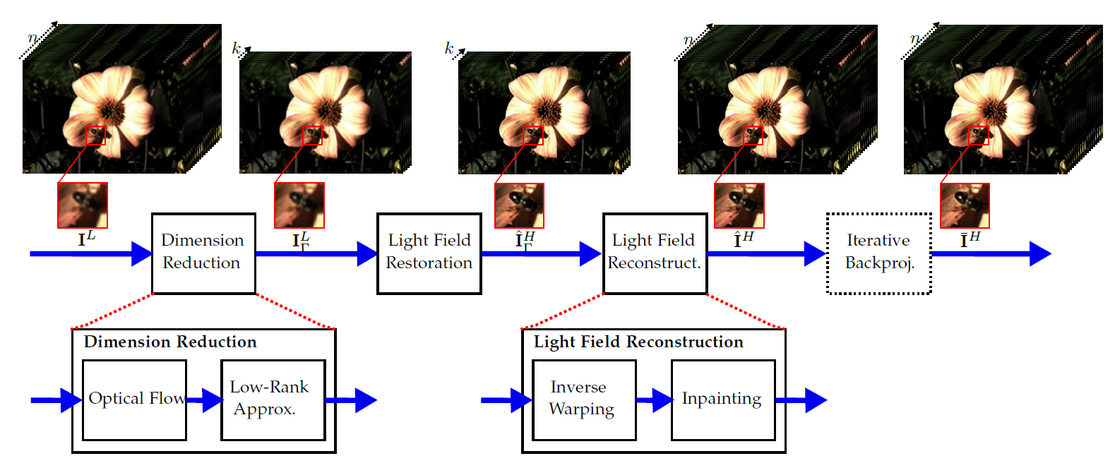
Figure 1: Block diagram of the proposed light field super-resolution method

3.1 Light Field Dimensionality Reduction

Many acquisition devices have been recently designed to capture light fields, including multi-sensor approaches [2], time-sequential capture methods [18, 19] and plenoptic cameras [1, 20]. All these different light field cameras have diverse spatial and angular specifications, which makes it very hard for a learning-based algorithm to learn a generalized model suitable to restore any kind of light field independent from the source. Moreover, a light field contains a huge amount of redundant information since it represents a different view of the same scene.

The authors in [21] hypothesized that this redundancy can be suppressed by jointly aligning the sub-aperture images in the light field and estimating a low-rank approximation (LRA) of the light field. This approach has shown very promising results in the field of light field compression. In the same spirit, the RASL algorithm [22] was used to find the homographies that globally align a batch of linearly correlated images. Both methods seek for an optimal set of homographies such that the matrix of aligned images can be decomposed in a low-rank matrix of aligned images, with the latter constraining the error matrix to be sparse. The results in Figure 2 show that while both RASL and LRA methods manage to globally align the sub-aperture images, the mean sub-aperture image is still very blurred, indicating that the light field is not suitably aligned.

The authors in [5] have used the block matching algorithm (BMA) to align patch volumes. The results in Figure 2 show that BMA manages to align better the sub-aperture images, where the average variance across the $n$ sub-aperture image is significantly reduced. This result suggests that local methods can improve the alignment of the sub-aperture images, which as we will see in the sequel, will allow us to significantly reduce the dimensionality of the light field.

No Align	RASL [22]	LRMA [21]	BMA	Horn-Scunk [23]	SIFT Flow [24]	CPM [25]	SPM-BP [26]
44.714	43.896	44.787	4.434	16.466	1.796	7.809	5.817
306.960	286.078	306.166	24.519	45.588	8.560	68.067	22.313
99.092	98.261	99.080	46.374	36.388	19.164	51.073	71.652

Figure 2: Cropped regions of the mean sub-aperture images when using different disparity compensation methods. Underneath each image we provide the average variance across the $n$ sub-aperture images which was used in [5] to characterize the performance of the alignment algorithm, where smaller values indicate better alignment.

In this paper, we formulate the light field dimensionality reduction problem as

$$\underset{\mathbf{u},\mathbf{v},\mathbf{A}}{min}{||\Gamma_{\mathbf{u},\mathbf{v}}\left(\mathbf{I}^{L}\right)-\mathbf{A}||^{2}_{2}\quad\text{ s.t. }\quad rank(\mathbf{A})=k}$$ (3)

where $\mathbf{u}\in\mathbb{R}^{m,n}$ and $\mathbf{v}\in\mathbb{R}^{m,n}$ are flow vectors that specify the displacement of each pixel needed to align each sub-aperture image with the centre view, $\mathbf{A}$ is a rank-$k$ matrix which approximates the aligned light field and $\Gamma_{\mathbf{u},\mathbf{v}}\left(\cdot\right)$ is a forward warping operator (which here performs a disparity compensation where the disparities maps $(\mathbf{u},\mathbf{v})$ are estimated with an optical flow estimator). This optimization problem is computationally intractable. Instead, we decompose this problem in two sub-problems: i) use optical flow to find the flow matrices $\mathbf{u}$ and $\mathbf{v}$ that best align each sub-aperture image with the centre view and ii) use low-rank approximation to derive the rank-$k$ matrix that minimizes the error with respect to the aligned light field.

3.1.1 Optical Flow

The problem of aligning all the sub-aperture images with the centre view can be formulated as

$$\mathbf{I}_{j}(x,y)=\mathbf{I}_{i}(x+\mathbf{u}_{i},y+\mathbf{v}_{i})\quad i\in\left[1,n\right](i\neq j)$$ (4)

where $j$ corresponds to the index of the centre view, and $\left(\mathbf{u}_{i},\mathbf{v}_{i}\right)$ are the flow vectors optimal to align the $i$-th sub-aperture image with the centre view. There are several optical flow algorithms intended to solve this problem [23, 24, 26, 25] where Figure 2 shows the performance of some of these methods. It can be seen that the mean aligned sub-aperture images computed using [23] is generally blurred while those aligned using the methods in [26, 25] generally provide ghosting artefacts at the edges. Moreover, it can be seen that SIFT Flow [24] generally provides very good alignment and manages to attain the smallest variation across the sub-aperture images. While the SIFT Flow algorithm will be used in this paper to compute the flow vectors, any other optical flow method can be used.

3.1.2 Low-Rank Approximation

Given that the flow-vectors $\left(\mathbf{u}_{i},\mathbf{v}_{i}\right)$ for the $i$-th sub-aperture image are already available, the minimization problem in Eq. (3) can now be reduced to

$$\underset{\mathbf{\mathbf{B}^{L},\mathbf{C}^{L}}}{min}{||\mathbf{I}^{L}_{\Gamma}-\mathbf{B}^{L}\mathbf{C}^{L}||^{2}_{2}}\quad\text{ s.t. }\quad rank(\mathbf{B}^{L})=k$$ (5)

where $\mathbf{I}^{L}_{\Gamma}=\Gamma_{\mathbf{u},\mathbf{v}}\left(\mathbf{I}^{L}\right)$, $\mathbf{B}^{L}\in\mathbb{R}^{m,k}$ is a rank-$k$ matrix and $\mathbf{C}^{L}\in\mathbb{R}^{k,n}$ is the combination weight matrix. These matrices can be found using singular value decomposition (SVD) $\mathbf{I}^{L}_{\Gamma}=\mathbf{U}\boldsymbol{\Sigma}\mathbf{V}^{T}$, where $\mathbf{B}^{L}$ is set as the $k$ first columns of $\mathbf{U}\boldsymbol{\Sigma}$ and $\mathbf{C}^{L}$ is set as the $k$ first rows of $\mathbf{V}^{T}$, so that $\mathbf{B}^{L}\mathbf{C}^{L}$ is the closest $k$-rank approximation of the aligned light field $\mathbf{I}^{L}_{\Gamma}$. The error matrix $\mathbf{E}^{L}$ is the error matrix which is simply computed using $\mathbf{E}^{L}=\mathbf{I}^{L}_{\Gamma}-\mathbf{B}^{L}\mathbf{C}^{L}$

Figure 3 depicts the performance of three different dimensionality reduction techniques at different ranks. To measure the dimensionality reduction ability of these methods we compute the root mean square error (RMSE) between the aligned original and the rank-$k$ representation of the aligned light field. It can be seen that the RASL algorithm has the largest distortions at almost all ranks when compared to the other two approaches. On the other hand, it can be seen that HLRA manages to significantly outperform the RASL method, which gain is attained by the improved alignment. Nevertheless, it can be clearly observed that the proposed Sift Flow + LRA method gives the best performance, especially at lower ranks, indicating that more information is captured within the low-rank matrix. To emphasize this point we show in figure 3 the principal basis of PCA, HLRA and Sift Flow + LRA. PCA is computed on the light field without disparity estimation and therefore can be considered here as a baseline to show that alignment allows us to get more information in the principal basis. Moreover, it can be seen that the principal basis derived using our Sift Flow + LRA manages to capture more texture detail in the principal basis than the other methods and confirms the benefit that local alignment has on the energy compaction ability of the proposed dimensionality reduction method.

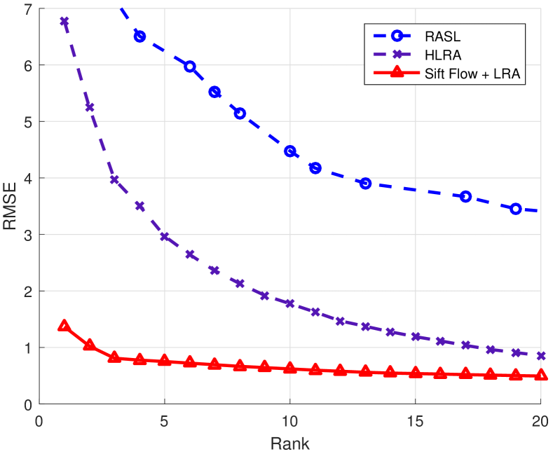
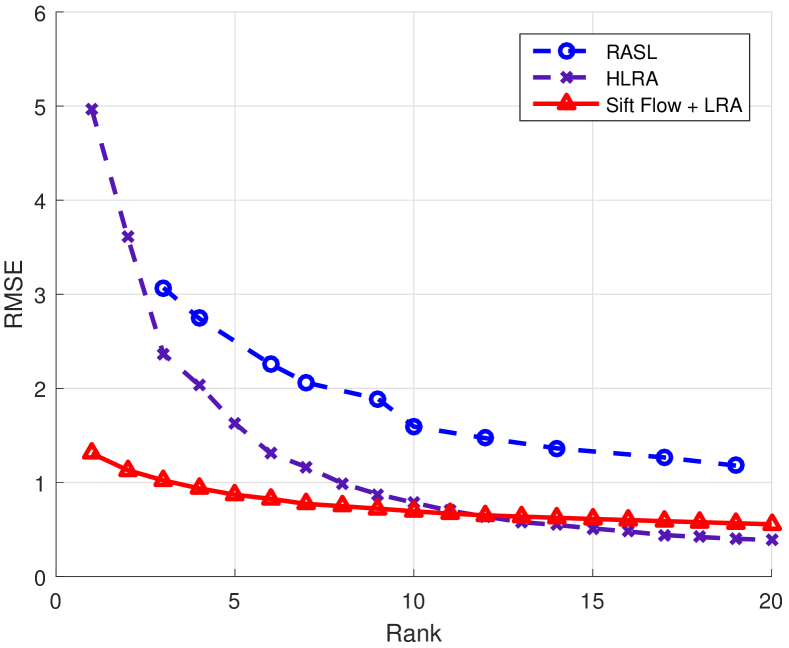
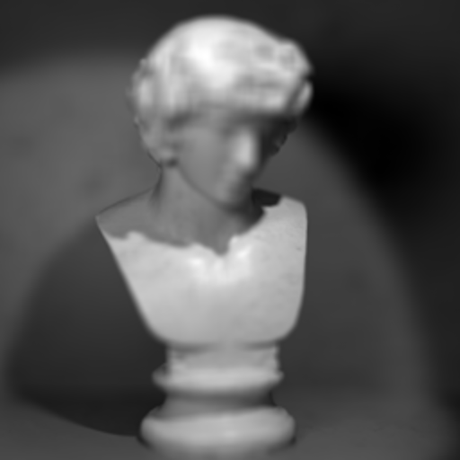
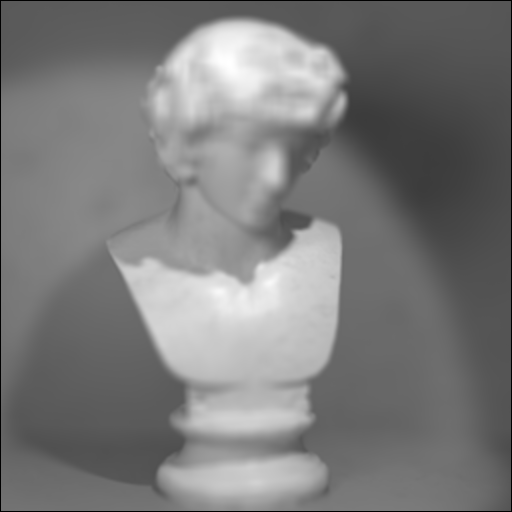
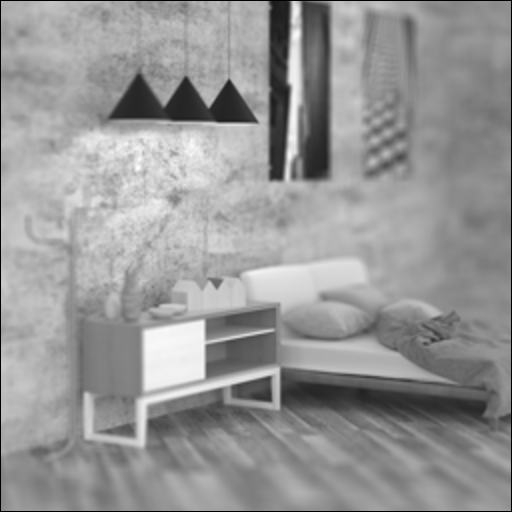
PCA	HLRA	Sift Flow + LRA	PCA	HLRA	Sift Flow + LRA

Figure 3: These figures show how the error between the low-rank and full rank representation vary at different ranks. It can be seen that using optical flow to align the light field followed by low-rank approximation attains the best performance. The images in the second row show the principal basis derived using different methods. The sharper the principal basis is the more information is being captured in the principal basis.

3.2 Light Field Restoration

We consider a low-rank representation of the aligned low-resolution light field $\mathbf{A}^{L}=\mathbf{B}^{L}\mathbf{C}^{L}$, where $\mathbf{A}^{L}\in\mathbb{R}^{m,n}$ is a rank-$k$ matrix with $k\ll n$. Similarly, $\mathbf{A}^{H}=\mathbf{B}^{H}\mathbf{C}^{H}$ is a rank-$k$ representation of the aligned high-resolution light field. The rank of a matrix is defined as the maximum number of linearly independent column vectors in the matrix. Moreover, the linearly dependent column vectors of a matrix can be reconstructed using a weighted summation of the linearly independent column vectors of the same matrix. This leads us to decompose $\mathbf{A}^{L}$ in two sub-matrices: $\breve{\mathbf{A}}^{L}\in\mathbb{R}^{m,k}$ which groups the linear independent column vectors of $\mathbf{A}^{L}$ and $\hat{\mathbf{A}}^{L}\in\mathbb{R}^{m,n-k}$ which groups the linearly dependent column vectors of $\mathbf{A}^{L}$. In practice, we decompose the rank-$k$ matrix $\mathbf{A}^{L}$ using QR decomposition (i.e. $\mathbf{A}^{L}=\mathbf{Q}\mathbf{R}$). The index of the linearly independent components of $\mathbf{A}^{L}$ then correspond to the index of the non-zero diagonal elements of the upper-triangular matrix $\mathbf{R}$. We then use the same indices to decompose $\mathbf{A}^{H}$ into sub-matrices $\breve{\mathbf{A}}^{H}$ and $\hat{\mathbf{A}}^{H}$. The matrix $\hat{\mathbf{A}}^{L}$ can be reconstructed as a linear combination of $\breve{\mathbf{A}}^{L}$, where the weight matrix $\mathbf{W}$ is computed using

$$\mathbf{W}=\left(\breve{\mathbf{A}}^{L\intercal}\breve{\mathbf{A}}^{L}\right)^{\dagger}\breve{\mathbf{A}}^{L\intercal}\hat{\mathbf{A}}^{L}$$ (6)

where $\left(\cdot\right)^{\dagger}$ stands for the pseudo inverse operator. We assume here that the weight matrix $\mathbf{W}$, which is optimal in terms of least squares to reconstruct $\hat{\mathbf{A}}^{L}$, is suitable to reconstruct $\hat{\mathbf{A}}^{H}$.

Driven by the recent success of deep learning in the field of single-image [27, 28] and light field super-resolution [10, 11], we use a DCNN to model the upscaling function that minimizes the following objective function

$$\nicefrac{{1}}{{2}}||\breve{\mathbf{A}}^{H}-f\left(\breve{\mathbf{A}}^{L}\right)||^{2}$$ (7)

where $f(\cdot)$ is a function modelled by the DCNN illustrated in Figure 4 which has ten convolutional layers. The linearly independent sub-matrix $\breve{\mathbf{A}}^{L}$ is passed through a stack of convolutional and rectified linear unit (ReLU) layers. We use a convolution stride of 1 pixel with no padding nor spatial pooling. The first convolutional layer has 64 filters of size $3\times 3\times k$ while the last layer, which is used to reconstruct the high-resolution light field, employs $k$ filter of size $3\times 3\times 64$. All the other layers use 64 filters of size $3\times 3\times 64$ which are initialized using the method in [29]. The DCNN was trained using a total of 200,000 random patch-volumes of size $64\times 64\times k$ from the 98 low- and high-resolution low-rank approximation of rank $k$ of the light fields from the EPFL, INRIA and HCI datasets. The Titan GTX1080Ti Graphical Processing Unit (GPU) was used to speed up the training process.

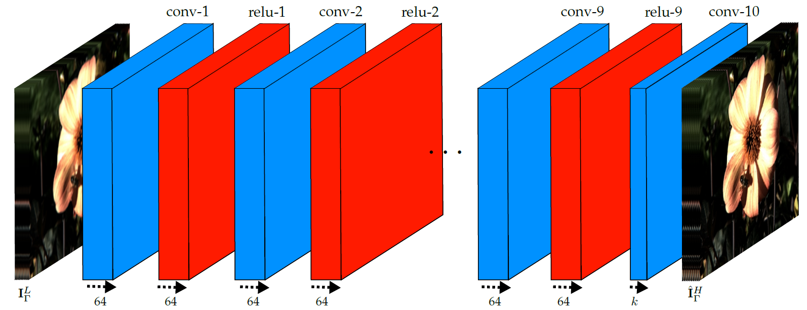
Figure 4: The proposed network structure which receives a low-resolution light field and restores it using the proposed DCNN.

During the evaluation phase, we estimate the super-resolved linearly independent representation of the light field $\breve{\mathbf{A}}^{H}=f\left(\breve{\mathbf{A}}^{L}\right)$. We then estimate the super-resolved linear dependent part of the light field using

$$\hat{\mathbf{A}}^{H}=\breve{\mathbf{A}}^{H}\mathbf{W}$$ (8)

The super-resolved low-rank representation of the aligned light field is then derived by the union of the two matrices $\hat{\mathbf{A}}^{H}$ and $\breve{\mathbf{A}}^{H}$ i.e. $\mathbf{A}^{H}=\hat{\mathbf{A}}^{H}\cup\breve{\mathbf{A}}^{H}$. The super-resolved light field is then reconstructed using

$$\hat{\mathbf{I}}^{H}_{\Gamma}=\mathbf{A}^{H}+\mathbf{E}^{L}$$ (9)

3.3 Light Field Reconstruction

The restored aligned light field $\hat{\mathbf{I}}^{H}_{\Gamma}$ has all sub-aperture images aligned with the centre view. A naïve approach to recover the original disparities of the restored sub-aperture images is to use forward warping. However, as can be seen in the first column of Figure 5(a), forward warping is not able to restore all pixels and results in a number of cracks or holes corresponding to occlusions (marked in green). One can use either bicubic interpolation or inverse warping to fill the holes. However, in case of occlusions, the neighbouring pixels may not be well correlated with the missing information, which often results in inaccurate estimations (see Figure 5(a) second column). More advanced inpainting algorithms [30, 31] can be used to restore each hole separately. However, these methods do not exploit the light field structure and therefore provide inconsistent reconstruction of the same spatial region at different angular views.

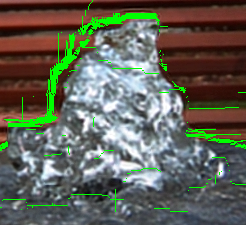
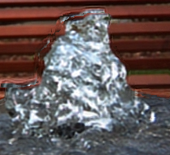
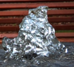
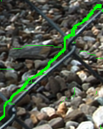
Forward Warping	Bicubic Interpolation	EPI Diffusion

(a) Inpainting the cracks marked in green

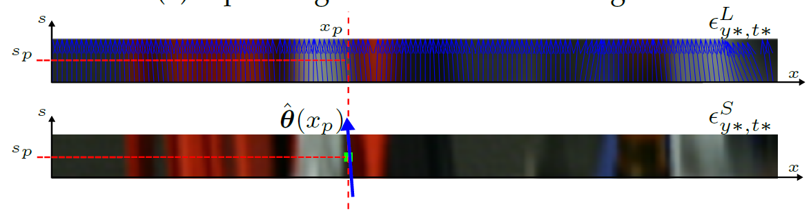
(b) Diffusion based inpainting

Figure 5: Filling the missing information caused by occlusion.

In this work, we use a diffusion based inpainting algorithm that estimates the missing pixels by diffusing information available in other views. Similar to the work in [32], we exploit the EPI structure to diffuse information along the dominant orientation of the EPI. However, instead of predicting the orientation of unknown pixels from their spatial neighborhood as done in [32], we exploit the similarity between the low- and super-resolved EPIs and use the structure tensor computed on the low-resolution EPI to guide the inpainting process in the high-resolution EPI.

Without loss of generality we consider the EPI where the dimensions $y\ast$ and $t\ast$ are fixed. The case of vertical slices is analogous. We first compute the structure tensor of the low-resolution EPI $\boldsymbol{\epsilon}^{L}_{y\ast,t\ast}$ at coordinates $(x,s)$ using

$$\mathbf{T}\left(x,s\right)=\nabla\boldsymbol{\epsilon}^{L}_{y\ast,t\ast}\left(x,s\right)\nabla\boldsymbol{\epsilon}^{L}_{y\ast,t\ast}\left(x,s\right)^{\intercal}$$ (10)

where $\nabla$ stands for the single order gradient computed using the sobel kernel. The authors in [32] compute an average weighting of the columns of $\mathbf{T}\left(x,s\right)$ to derive the dominant orientation, where the weights are given by an anisotropy measure. Nevertheless, the anisotropy may fail in regions that are smooth and therefore the weighted average may fail in these regions to estimate the dominant direction of the EPI. This problem becomes an issue when computing these orientations on low-resolution versions of the light fields. Instead, we estimate the orientation at every pixel in the EPI by computing the eigen decomposition of $\mathbf{T}\left(x,s\right)$ and choose the direction $\boldsymbol{\theta}\left(x,s\right)$ which corresponds to the eigen-vector with the smallest eigen-value. Moreover, driven by the observation that the disparities in a light field are typically small, and considering that the local slope in the EPI is proportional to the disparity, it is reasonable to assume that slopes which correspond to large disparities are less probable to occur. Therefore, to ensure that the tensor driven diffusion is performed along a single coherent direction per column of the EPI and reduce noise, the dominant orientation $\boldsymbol{\theta}\left(x\right)$ is computed using the column-wise median of $\boldsymbol{\theta}\left(x,s\right)$ whose orientation is in the range $[\frac{\pi}{2}-\alpha,\frac{\pi}{2}+\alpha]$ radians. In all our experiments we set $\alpha=$ $\pi\text{/}4\text{\,}\mathrm{rad}$. While the dominant orientation vectors are less noisy, we further reduce the noise by applying the Total Variation (TV-L1) denoising [33] on the orientation field $\boldsymbol{\theta}\left(x\right)$, which searches to optimize

$$\hat{\boldsymbol{\theta}}=arg\,min_{\hat{\boldsymbol{\theta}}}{||\nabla\hat{\boldsymbol{\theta}}||_{1}+\lambda||\hat{\boldsymbol{\theta}}-\boldsymbol{\theta}||_{2}}$$ (11)

where $\lambda$ is the total variation regularization parameter and was set to 0.5 in our experiments. Figure 5(b) (top) shows the EPI of the low-resolution light field $\boldsymbol{\epsilon}^{L}_{y\ast,t\ast}$ and the dominant orientations $\hat{\boldsymbol{\theta}}\left(x\right)$ marked by blue arrows.

The restored EPI $\boldsymbol{\epsilon}^{H}_{y\ast,t\ast}:=\hat{\mathbf{I}}^{H}(x,y\ast,s,t\ast)$ (see Figure 5(b) (bottom)) has a number of missing pixels (marked in green). Consider that the hole we want to inpaint has coordinates $\left(x_{p},s_{p}\right)$. The aim of the proposed diffusion based inpainting algorithm is to propagate known pixels in the orientation $\hat{\boldsymbol{\theta}}\left(x_{p}\right)$ to fill the missing pixels. The diffusion over the EPI $\boldsymbol{\epsilon}^{H}_{y\ast,t\ast}$ evolves as

$$\frac{\partial\boldsymbol{\epsilon}^{H}_{y\ast,t\ast}}{\partial s}=\mathrm{Tr}\hskip 1.0pt\left(\hat{\boldsymbol{\theta}}\left(x_{p}\right)\hat{\boldsymbol{\theta}}\left(x_{p}\right)^{\intercal}\mathbf{H}\left(x_{p},s_{p}\right)\right)$$ (12)

where $\mathrm{Tr}\left(\cdot\right)$ stands for the trace operator and $\mathbf{H}\left(x,s\right)$ denotes the Hessian of $\boldsymbol{\epsilon}^{H}_{y\ast,t\ast}$ at coordinates $\left(x,s\right)$. The term $\hat{\boldsymbol{\theta}}\left(x_{p}\right)\hat{\boldsymbol{\theta}}\left(x_{p}\right)^{\intercal}$ is used to enforce the diffusion to occur only in the direction of the isophote eigenvector. The missing pixels are restored iteratively by finding the solution to (12) which is closest to zero. Figure 5(a) (third column) shows the results attained using the proposed inpainting strategy.

In order to restore all the cracks in the light field we first fix $t\ast$ to that of the center view and iteratively restore all the horizontal EPIs for all $y\ast\in[1,Y]$ by solving Eq. (12). This corresponds to filling the cracks for the centre row of the matrix of sub-aperture images. We then fix $s\ast$ to that of the centre view and iteratively restore all the vertical EPIs for all $x\ast\in[1,X]$ which effectively restores all cracks for the centre column of the matrix of sub-aperture images. The remaining propagations are performed row-by-row where each time we restore all pixels within $t\ast\in[1,Q]$.

3.4 Iterative Back-Projection

One problem with the method proposed in this paper is that after we restore the aligned light field $\hat{\mathbf{I}}^{H}_{\Gamma}$ we have to compute inverse warping to restore the original disparities. However, the inverse warping is not able to recover occluded regions and some pixels are displaced by $\raise 1.18056pt\hbox{\set@color$\scriptstyle\pm$}1$-pixel due to rounding errors. While the former problem is solved using the method described in Section 3.3, the second problem was not yet addressed. Nevertheless, the results illustrated in Tables I, II and Figure 6 indicate that significant performance gains can be achieved even if we do not explicitly cater for distortions caused by rounding errors in the inverse warping process. Nevertheless, these distortions can be corrected using the classical method of iterative back projection [34], which is adopted by several single image super-resolution methods (see [35]) to ensure that the down sampled version of the super-resolved light field is consistent with the observed low-resolution light field. The IBP algorithm iteratively refines the estimated high-resolution light field $\bar{\mathbf{I}}^{H}_{\kappa}$ at iteration $\kappa$ by first back-projecting it into an estimated low-resolution light field $\bar{\mathbf{I}}^{L}_{\kappa}$ using

$$\bar{\mathbf{I}}^{L}_{\kappa}=\mathbf{\uparrow}_{\alpha}\left(\mathbf{\downarrow}_{\alpha}\mathbf{B}\bar{\mathbf{I}}^{H}_{\kappa}\right)$$ (13)

where $\mathbf{\downarrow}_{\alpha}$ is a downsampling operator, $\mathbf{\uparrow}_{\alpha}$ is the bicubic upscaling operation, $\alpha$ is the magnification factor and $\mathbf{B}$ is the blurring kernel. The deviation between the LR views found by back-projection and the original LR views is then used to further correct each HR estimated view of the light field as

$$\bar{\mathbf{I}}^{H}_{\kappa+1}=\bar{\mathbf{I}}^{H}_{\kappa}+\left(\mathbf{I}^{L}-\bar{\mathbf{I}}^{L}_{\kappa}\right)$$ (14)

The IBP algorithm is initiated by setting $\bar{\mathbf{I}}^{H}_{0}=\hat{\mathbf{I}}^{H}$ and the iterative procedure terminates when $\kappa=K$. It was observed that significant improvements were achieved in the first few iterations and we therefore set $K=10$ in our experiments. The restored light field following iterative back-projection is therefore set to $\bar{\mathbf{I}}^{H}=\bar{\mathbf{I}}^{H}_{K}$.

4 Experimental Results

The experiments conducted in this paper use both synthetic and real-world light fields from publicly available datasets. We use 98 light fields from the EPFL [36], INRIA and HCI for training. We conducted the tests using light fields from the INRIA and Stanford datasets. We use the Stanford dataset in this evaluation since it has disparities significantly larger than both INRIA and EPFL light fields, which were captured using plenoptic cameras. Moreover, unlike the HCI dataset, the Stanford light fields capture real world objects. We therefore use this dataset to assess the generalization ability of the algorithms considered in this experiment to light fields which are captured using camera sensors which differ from the ones used for training. While the sub-aperture images of the EPFL, HCI and Stanford datasets are available, the light fields in the INRIA dataset were decoded using the method in [37] as mentioned on their website. In all our experiments we consider a $9\times 9$ array of sub-aperture images. For computational purposes, the high-resolution images of the Stanford dataset were downscaled such that the lowest dimension is set to 400 pixels. The high-resolution images of the other datasets were kept unchanged, i.e. $512\times 512$ for the HCI light fields and $625\times 434$ for both EPFL and INRIA light fields. Unless otherwise specified, the low-resolution light fields were generated by blurring each high-resolution sub-aperture image with a Gaussian filter using a window size of 7 and standard deviation of 1.6, down-sampled to the desired resolution and up-scaled back to the target resolution using bi-cubic interpolation. Unless otherwise specified, the iterative back-projection refinement strategy was disabled to permit a fair comparison to the other state of the art super-resolution methods considered.

We compare the performance of our system against the best performing methods found in our recent work [5], namely the CNN based light field super-resolution algorithm (LF-SRCNN) [11] and both linear subspace projection based methods, PCA+RR and BM+PCA+RR [5]. These methods were retrained using samples from the 98 training light fields mentioned above using training procedures explained in their respective papers. Moreover, given that the very deep super-resolution (VDSR) method [28] achieved state-of-the-art performance on single image super-resolution, we apply this method to restore every sub-aperture image independently. It is important to mention here that in our previous work we found that BM+PCA+RR significantly outperforms several other light field and single-image super-resolution algorithms including [10, 8, 38, 39, 40, 41, 27]. Due to space constraints we did not provide comparisons against the latter approaches.

The results in table I and table II compare these super-resolution methods in terms of PSNR for magnification factors of $\times 2$ and $\times 3$ respectively. Moreover, the results in Figure 6 show the centre views of light fields restored using these methods when considering a magnification factor of $\times 3$. The VDSR algorithm [28] achieves on average a PSNR gain of 0.33 dB over bicubic interpolation. One major limitation of VDSR is that it does not exploit the light field structure where each sub-aperture image is being restored independently. The PCA+RR algorithm [5] manages to restore more texture detail and is particularly effective to restore light fields with small disparities, which is the case of the INRIA light fields. This can be attributed to the fact that the PCA+RR does not compensate for disparities and therefore is not able to generalize to light fields containing disparities which were not considered during training, which is the case for the Stanford light fields. In fact the Stanford light fields restored using PCA+RR contain blocking artefacts. The BM+PCA+RR method [5] extends this method by aligning the patch-volumes using block-matching. This results in a more generalized method that achieves average PSNR gains of 2.52 dB and 1.76 dB over bi-cubic on the INRIA and Stanford light fields respectively. Nevertheless, the light fields restored using this method may contain some artefacts especially near the edges.

TABLE I: PSNR using different light field super-resolution algorithms when considering a magnification factor of $\times 2$. For clarity bold blue marks the highest and bold red indicates the second highest score.

Light Field Name	Bicubic	PCA+RR [5]	BM+PCA+RR [5]	LF-SRCNN [11]	VDSR [28]	Proposed
Bee 2 (INRIA)	30.1673	34.1579	33.4655	33.8268	30.4027	33.4915
Dist. Church (INRIA)	24.3059	26.5071	26.4571	25.9930	24.5419	26.7502
Duck (INRIA)	23.5394	26.7401	26.2528	26.0713	23.8371	26.3777
Framed (INRIA)	27.5974	30.7093	30.4965	30.0697	27.8725	30.5365
Fruits (INRIA)	28.4907	31.7884	32.0002	31.6820	28.7827	32.0789
Mini (INRIA)	27.6332	30.4751	30.0867	29.8941	27.9175	30.1601
Rose (INRIA)	33.5436	37.0791	36.9566	36.8245	33.7943	36.8416
Amethyst (STANFORD)	30.5227	32.5139	32.4262	32.2953	30.8360	32.2737
Bracelet (STANFORD)	26.4662	23.8183	28.2356	28.8858	26.8523	29.4046
Chess (STANFORD)	30.2895	31.9292	32.5708	32.1922	30.6313	32.6123
Eucalyptus (STANFORD)	30.7865	32.4162	32.4900	32.1989	31.0431	32.6205
Lego Gantry (STANFORD)	27.6235	28.0729	28.7230	29.8086	27.9998	29.8112
Lego Knights (STANFORD)	27.3794	27.8457	29.4664	29.5354	27.7446	29.3177

TABLE II: PSNR using different light field super-resolution algorithms when considering a magnification factor of $\times 3$. For clarity bold blue marks the highest and bold red indicates the second highest score.

Light Field Name	Bicubic	PCA+RR [5]	BM+PCA+RR [5]	LF-SRCNN [11]	VDSR [28]	Proposed
Bee 2 (INRIA)	27.8623	31.2436	31.1886	31.3945	28.2457	31.2545
Dist. Church (INRIA)	23.3138	24.7103	24.6220	24.5874	23.7707	24.6535
Duck (INRIA)	22.0702	23.9844	23.8083	24.0623	22.5350	24.1549
Framed (INRIA)	26.1627	28.0771	28.1587	27.9157	26.8462	28.2954
Fruits (INRIA)	26.5269	29.0908	29.1969	29.2100	26.9021	29.5297
Mini (INRIA)	26.3035	28.4265	28.3212	28.1731	26.7192	28.4009
Rose (INRIA)	31.7687	34.4692	34.5754	34.3064	32.0424	34.3392
Amethyst (STANFORD)	29.0665	31.0848	31.1184	30.5971	29.5618	30.4628
Bracelet (STANFORD)	24.1221	22.2654	25.3946	26.1013	24.3484	26.2712
Chess (STANFORD)	27.3679	29.5207	29.6773	30.0278	27.6514	30.1485
Eucalyptus (STANFORD)	29.2136	31.3459	31.3547	30.9433	29.4650	31.1772
Lego Gantry (STANFORD)	24.6721	25.3941	25.6383	26.8054	24.7923	26.9466
Lego Knights (STANFORD)	24.0182	24.4944	25.5768	26.0771	24.1256	26.1358

Original	Bicubic	PCA+RR [5]	BM+PCA+RR [5]	LF-SRCNN [11]	VDSR [28]	Proposed

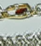
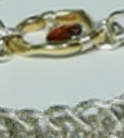
Figure 6: Restored center view using different light field super-resolution algorithms. These are best viewed in color and by zooming on the views.

The LF-SRCNN method [11], which uses deep learning to restore each sub-aperture image independently, was found to achieve a marginal gain over BM+PCA+RR (0.05 dB). While, light fields restored using LF-SRCNN generally contain less artefacts compared to BM+PCA+RR, they risk to restore light fields which are angularly incoherent. Nevertheless, our method achieves the best performance achieving an overall gain of 0.2 dB over the second-best performing algorithm LF-SRCNN. This performance gain is more evident in the subjective results illustrated in Figure 6 where the restored light fields are sharper and are visually more pleasing.

As mentioned in section 3.4, one problem with the proposed method is that the inverse warping is unable to perfectly restore the original disparities of the light field. Nevertheless, the results in tables I, II and Figure 6 clearly show that our proposed method outperforms the other schemes even without the use of the iterative back-projection refinement strategy.

In order to fairly assess the contribution of iterative back-projection, we apply it as a post process for the two best performing methods, namely LF-SRCNN and our proposed scheme LR-LFSR. Tables III and IV show the performance of the two best performing methods with and without iterative back projection as a post-processing step at magnification factors of $\times 2$ and $\times 3$ respectively. It can be immediately noticed that IBP significantly improves the quality of both methods. Nevertheless, our method which uses iterative back projection as a post-processing step achieves the best performance achieving PSNR gains of 0.41 dB and 0.31 dB at magnification factors of $\times 2$ and $\times 3$ respectively over LF-SRCNN followed by iterative back projection. It is important to notice that while the performance gain of our method over LF-SRCNN without IBP is around 0.23 dB and 0.12 dB at magnification factors of $\times 2$ and $\times 3$ respectively, this gain roughly doubles when both use IBP as a post processing step. This indicates that since LF-SRCNN processes each view independently, IBP only corrects inconsistencies between the low-resolution and restored light fields. Apart from this distortion, LR-LFSR-IBP corrects the distortions caused by the inverse warping process which provides light fields which are more visually pleasing and with smoother transitions across views. Supplementary multimedia files uploaded on ScholarOne show some sample restored light field. Supplementary material is available on the project’s website while the code of the LR-LFSR will be made available upon publication.

TABLE III: PSNR obtained with the best two methods at a magnification of $\times 2$ with and without iterative back projection as a post process.

Light Field Name	Bicubic	LF-SRCNN	LF-SRCNN-IBP	LR-LFSR	LR-LFSR-IBP
Bee 2 (INRIA)	30.1673	33.8268	34.7257	33.4915	35.0306
Dist. Church (INRIA)	24.3059	25.9930	26.7415	26.7502	27.1527
Duck (INRIA)	23.5394	26.0713	27.293	26.3777	27.6928
Framed (INRIA)	27.5974	30.0697	31.0592	30.5365	31.7185
Fruits (INRIA)	28.4907	31.6820	32.6581	32.0789	33.3370
Mini (INRIA)	27.6332	29.8941	30.5193	30.1601	30.9899
Rose (INRIA)	33.5436	36.8245	37.4991	36.8416	37.8970
Amethyst (STANFORD)	30.5227	32.2953	33.5662	32.2737	33.8686
Bracelet (STANFORD)	26.4662	28.8858	30.6367	29.4046	30.9579
Chess (STANFORD)	30.2895	32.1922	33.6715	32.6123	34.1438
Eucalyptus (STANFORD)	30.7865	32.1989	33.0700	32.6205	33.4550
Lego Gantry (STANFORD)	27.6235	29.8086	31.5071	29.8112	31.8631
Lego Knights (STANFORD)	27.3794	29.5354	31.2148	29.3177	31.3240

TABLE IV: PSNR obtained with the best two methods at a magnification of $\times 3$ with and without iterative back projection as a post process.

Light Field Name	Bicubic	LF-SRCNN	LF-SRCNN-IBP	LR-LFSR	LR-LFSR-IBP
Bee 2 (INRIA)	27.8623	31.3945	32.4662	31.2545	32.7661
Dist. Church (INRIA)	23.3138	24.5874	25.2440	24.6535	25.1669
Duck (INRIA)	22.0702	24.0623	24.7698	24.1549	25.0554
Framed (INRIA)	26.1627	27.9157	28.9111	28.2954	29.5017
Fruits (INRIA)	26.5269	29.2100	30.1651	29.5297	30.7844
Mini (INRIA)	26.3035	28.1731	28.6895	28.4009	29.1335
Rose (INRIA)	31.7687	34.3064	34.9356	34.3392	35.4656
Amethyst (STANFORD)	29.0665	30.5971	31.5991	30.4628	31.8143
Bracelet (STANFORD)	24.1221	26.1013	27.0010	26.2712	27.3423
Chess (STANFORD)	27.3679	30.0279	31.1502	30.1485	31.4388
Eucalyptus (STANFORD)	29.2136	30.9433	31.5263	31.1772	31.9161
Lego Gantry (STANFORD)	24.6721	26.8054	27.8395	26.9466	27.8852
Lego Knights (STANFORD)	24.0182	26.0771	27.6550	26.1358	27.7168

5 Conclusion

In this paper, we have proposed a novel spatial light field super-resolution algorithm able to reconstruct high quality coherent light fields. We have shown that the information in a light field can be efficiently compacted by aligning the sub-aperture images using optical flow followed by low-rank matrix approximation. The low rank approximation of the aligned light field gives an embedding in a lower dimensional space which is super-resolved using deep learning. All aligned views of the high-resolution light field can be reconstructed from the super-resolved embedding by simple linear combinations. These views are then inverse warped to restore the disparities of the original light field. Holes corresponding to dis-occlusions or cracks resulting from the inverse warping are filled in using a novel diffusion based inpainting algorithm which diffuses known pixels in the EPI along dominant orientations computed in the low-resolution EPI.

Extensive simulations show that the proposed method manages to generalize well, i.e. manages to successfully restore light fields whose disparities are considerably different from those used during training. These results also show that our proposed method is competitive and most of the time superior to existing state-of-the-art light field super-resolution algorithms, including a recent approach which adopts deep learning to restore each sub-aperture image independently. One major limitation of the proposed scheme is that the inverse warping process is not able to restore the original disparities and produces some distortion caused by rounding errors. We proposed here to use the classical iterative back-projection as a post processing step. Simulation results clearly show the benefit of using IBP as a post processing of the super-resolved light field and demonstrate that the proposed method with IBP achieves the best performance, outperforming LF-SRCNN followed by IBP by 0.4 dB.

References

- [1] R. Ng, M. Levoy, M. Brédif, G. Duval, M. Horowitz, and P. Hanrahan, “Light Field Photography with a Hand-Held Plenoptic Camera,” Tech. Rep., Apr. 2005. [Online]. Available: http://graphics.stanford.edu/papers/lfcamera/
- [2] B. Wilburn, N. Joshi, V. Vaish, E.-V. Talvala, E. Antunez, A. Barth, A. Adams, M. Horowitz, and M. Levoy, “High performance imaging using large camera arrays,” ACM Trans. Graph., vol. 24, no. 3, pp. 765–776, Jul. 2005. [Online]. Available: http://doi.acm.org/10.1145/1073204.1073259
- [3] G. Wu, B. Masia, A. Jarabo, Y. Zhang, L. Wang, Q. Dai, T. Chai, and Y. Liu, “Light field image processing: An overview,” IEEE Journal of Selected Topics in Signal Processing, vol. PP, no. 99, pp. 1–1, 2017.
- [4] C.-K. Liang and R. Ramamoorthi, “A light transport framework for lenslet light field cameras,” ACM Trans. Graph., vol. 34, no. 2, pp. 16:1–16:19, Mar. 2015. [Online]. Available: http://doi.acm.org/10.1145/2665075
- [5] R. A. Farrugia, C. Galea, and C. Guillemot, “Super resolution of light field images using linear subspace projection of patch-volumes,” IEEE Journal of Selected Topics in Signal Processing, vol. PP, no. 99, pp. 1–1, 2017.
- [6] A. Levin, W. Freeman, and F. Durand, “Understanding camera trade-offs through a bayesian analysis of light field projections,” in European Conference on Computer Vision (ECCV), Oct. 2008.
- [7] T. E. Bishop and P. Favaro, “The light field camera: Extended depth of field, aliasing, and superresolution,” IEEE Transactions on Pattern Analysis and Machine Intelligence, vol. 34, no. 5, pp. 972–986, May 2012.
- [8] K. Mitra and A. Veeraraghavan, “Light field denoising, light field superresolution and stereo camera based refocussing using a gmm light field patch prior,” in 2012 IEEE Computer Society Conference on Computer Vision and Pattern Recognition Workshops, June 2012, pp. 22–28.
- [9] S. Wanner and B. Goldluecke, “Variational light field analysis for disparity estimation and super-resolution,” IEEE Transactions on Pattern Analysis and Machine Intelligence, vol. 36, no. 3, pp. 606–619, March 2014.
- [10] Y. Yoon, H.-G. Jeon, D. Yoo, J.-Y. Lee, and I. S. Kweon, “Learning a deep convolutional network for light-field image super-resolution,” in IEEE Conference on Computer Vision and Pattern Recognition (CVPR), June 2015, pp. 57–65.
- [11] Y. Yoon, H. G. Jeon, D. Yoo, J. Y. Lee, and I. S. Kweon, “Light-field image super-resolution using convolutional neural network,” IEEE Signal Processing Letters, vol. 24, no. 6, pp. 848–852, June 2017.
- [12] N. K. Kalantari, T.-C. Wang, and R. Ramamoorthi, “Learning-based view synthesis for light field cameras,” ACM Transactions on Graphics (Proceedings of SIGGRAPH Asia 2016), vol. 35, no. 6, 2016.
- [13] G. Wu, M. Zhao, L. Wang, Q. Dai, T. Chai, and Y. Liu, “Light field reconstruction using deep convolutional network on epi,” in IEEE Computer Society Conference on Computer Vision and Pattern Recognition (CVPR), July 2017.
- [14] T.-C. Wang, J.-Y. Zhu, N. K. Kalantari, A. A. Efros, and R. Ramamoorthi, “Light field video capture using a learning-based hybrid imaging system,” ACM Transactions on Graphics (Proceedings of SIGGRAPH), vol. 36, no. 4, 2017.
- [15] Y. Wang, Y. Liu, W. Heidrich, and Q. Dai, “The light field attachment: Turning a dslr into a light field camera using a low budget camera ring,” IEEE Transactions on Visualization and Computer Graphics, vol. 23, no. 10, pp. 2357–2364, Oct 2017.
- [16] M. Levoy and P. Hanrahan, “Light field rendering,” in Proceedings of the 23rd Annual Conference on Computer Graphics and Interactive Techniques, ser. SIGGRAPH ’96. New York, NY, USA: ACM, 1996, pp. 31–42. [Online]. Available: http://doi.acm.org/10.1145/237170.237199
- [17] S. J. Gortler, R. Grzeszczuk, R. Szeliski, and M. F. Cohen, “The lumigraph,” in Proceedings of the 23rd Annual Conference on Computer Graphics and Interactive Techniques, ser. SIGGRAPH ’96. New York, NY, USA: ACM, 1996, pp. 43–54. [Online]. Available: http://doi.acm.org/10.1145/237170.237200
- [18] C. Kim, H. Zimmer, Y. Pritch, A. Sorkine-Hornung, and M. Gross, “Scene reconstruction from high spatio-angular resolution light fields,” ACM Trans. Graph., vol. 32, no. 4, pp. 73:1–73:12, Jul. 2013. [Online]. Available: http://doi.acm.org/10.1145/2461912.2461926
- [19] Y. Taguchi, A. Agrawal, S. Ramalingam, and A. Veeraraghavan, “Axial light field for curved mirrors: Reflect your perspective, widen your view,” in 2010 IEEE Computer Society Conference on Computer Vision and Pattern Recognition, June 2010, pp. 499–506.
- [20] A. Veeraraghavan, R. Raskar, A. Agrawal, A. Mohan, and J. Tumblin, “Dappled photography: Mask enhanced cameras for heterodyned light fields and coded aperture refocusing,” ACM Trans. Graph., vol. 26, no. 3, Jul. 2007. [Online]. Available: http://doi.acm.org/10.1145/1276377.1276463
- [21] X. Jiang, M. L. Pendu, R. A. Farrugia, and C. Guillemot, “Light field compression with homography-based low rank approximation,” IEEE Journal of Selected Topics in Signal Processing, vol. PP, no. 99, pp. 1–1, 2017.
- [22] Y. Peng, A. Ganesh, J. Wright, W. Xu, and Y. Ma, “Rasl: Robust alignment by sparse and low-rank decomposition for linearly correlated images,” in 2010 IEEE Computer Society Conference on Computer Vision and Pattern Recognition, June 2010, pp. 763–770.
- [23] B. K. Horn and B. G. Schunck, “Determining optical flow,” Cambridge, MA, USA, Tech. Rep., 1980.
- [24] C. Liu, J. Yuen, and A. Torralba, “Sift flow: Dense correspondence across scenes and its applications,” IEEE Transactions on Pattern Analysis and Machine Intelligence, vol. 33, no. 5, pp. 978–994, May 2011.
- [25] Y. Hu, R. Song, and Y. Li, “Efficient coarse-to-fine patch match for large displacement optical flow,” in 2016 IEEE Conference on Computer Vision and Pattern Recognition (CVPR), June 2016, pp. 5704–5712.
- [26] Y. Li, D. Min, M. S. Brown, M. N. Do, and J. Lu, “Spm-bp: Sped-up patchmatch belief propagation for continuous mrfs,” in 2015 IEEE International Conference on Computer Vision (ICCV), Dec 2015, pp. 4006–4014.
- [27] C. Dong, C. C. Loy, K. He, and X. Tang, “Image super-resolution using deep convolutional networks,” IEEE Trans. Pattern Anal. Mach. Intell., vol. 38, no. 2, pp. 295–307, Feb. 2016. [Online]. Available: http://dx.doi.org/10.1109/TPAMI.2015.2439281
- [28] J. Kim, J. K. Lee, and K. M. Lee, “Accurate image super-resolution using very deep convolutional networks,” in 2016 IEEE Conference on Computer Vision and Pattern Recognition (CVPR), June 2016, pp. 1646–1654.
- [29] X. Glorot and Y. Bengio, “Understanding the difficulty of training deep feedforward neural networks,” in Proceedings of the Thirteenth International Conference on Artificial Intelligence and Statistics (AISTATS-10), Y. W. Teh and D. M. Titterington, Eds., vol. 9, 2010, pp. 249–256. [Online]. Available: http://www.jmlr.org/proceedings/papers/v9/glorot10a/glorot10a.pdf
- [30] A. Criminisi, P. Perez, and K. Toyama, “Region filling and object removal by exemplar-based image inpainting,” Trans. Img. Proc., vol. 13, no. 9, pp. 1200–1212, Sep. 2004. [Online]. Available: http://dx.doi.org/10.1109/TIP.2004.833105
- [31] Z. Xu and J. Sun, “Image inpainting by patch propagation using patch sparsity,” IEEE Transactions on Image Processing, vol. 19, no. 5, pp. 1153–1165, May 2010.
- [32] O. Frigo and C. Guillemot, “Epipolar plane diffusion: An efficient approach for light field editing,” London, France, Sep. 2017.
- [33] L. I. Rudin, S. Osher, and E. Fatemi, “Nonlinear total variation based noise removal algorithms,” Physica D: Nonlinear Phenomena, vol. 60, no. 1, pp. 259 – 268, 1992. [Online]. Available: http://www.sciencedirect.com/science/article/pii/016727899290242F
- [34] M. Irani and S. Peleg, “Improving resolution by image registration,” CVGIP: Graphical Models and Image Processing, vol. 53, no. 3, pp. 231 – 239, 1991. [Online]. Available: http://www.sciencedirect.com/science/article/pii/104996529190045L
- [35] D. Glasner, S. Bagon, and M. Irani, “Super-resolution from a single image,” in 2009 IEEE 12th International Conference on Computer Vision, Sept 2009, pp. 349–356.
- [36] M. Rerabek and T. Ebrahimi, “New light field image dataset,” in Int. Conf. on Quality of Experience, 2016.
- [37] D. G. Dansereau, O. Pizarro, and S. B. Williams, “Decoding, calibration and rectification for lenselet-based plenoptic cameras,” in 2013 IEEE Conference on Computer Vision and Pattern Recognition, June 2013, pp. 1027–1034.
- [38] T. Peleg and M. Elad, “A statistical prediction model based on sparse representations for single image super-resolution,” IEEE Transactions on Image Processing, vol. 23, no. 6, pp. 2569–2582, June 2014.
- [39] C. Dong, C. C. Loy, K. He, and X. Tang, “Image super-resolution using deep convolutional networks,” IEEE Transactions on Pattern Analysis and Machine Intelligence, vol. 38, no. 2, pp. 295–307, Feb 2016.
- [40] K. Zhang, B. Wang, W. Zuo, H. Zhang, and L. Zhang, “Joint learning of multiple regressors for single image super-resolution,” IEEE Signal Processing Letters, vol. 23, no. 1, pp. 102–106, Jan 2016.
- [41] R. Timofte, V. De, and L. V. Gool, “Anchored neighborhood regression for fast example-based super-resolution,” in 2013 IEEE International Conference on Computer Vision, Dec 2013, pp. 1920–1927.