Energy spectrum of tearing mode turbulence in sheared background field

Abstract

The energy spectrum of tearing mode turbulence in a sheared background magnetic field is studied in this work. We consider the scenario where the nonlinear interaction of overlapping large-scale modes excites a broad spectrum of small-scale modes, generating tearing mode turbulence. The spectrum of such turbulence is of interest since it is relevant to the small-scale back-reaction on the large-scale field. The turbulence we discuss here differs from traditional MHD turbulence mainly in two aspects. One is the existence of many linearly stable small-scale modes which cause an effective damping during energy cascade. The other is the scale-independent anisotropy induced by the large-scale modes tilting the sheared background field, as opposed to the scale-dependent anisotropy frequently encountered in traditional critically balanced turbulence theories. Due to these two differences, the energy spectrum deviates from a simple power law and takes the form of a power law multiplied by an exponential falloff. Numerical simulations are carried out using visco-resistive MHD equations to verify our theoretical predictions, and reasonable agreement is found between the numerical results and our model.

I Introduction

The generation of a spectrum of small-scale tearing modes by their large-scale counterparts is a very relevant issue both in magnetically confined devices such as a reversed-field-pinch (RFP) or a tokamak as well as in space and astrophysical plasmas. For RFPs, the constant interaction of tearing modes and resistive interchange modes keeps the plasma in a perpetual turbulent state RFP . For tokamaks, the non-linear excitation and overlapping of a spectrum of tearing modes may break nested flux surfaces and lead to disruption Diamond1984 ; Strauss1986 ; Craddock1991 . In astrophysical plasmas, secondary plasmoid turbulence is found to play a crucial role during magnetic reconnection both in kinetic Daughton2011 and in resistive MHDHuang16APJ investigations.

An important aspect of these problems is the back-reaction of small-scale field fluctuations on their large-scale counterparts. A well-known example of such back-reaction is the hyper-resistivity produced in a mean-field theory, which has been a subject of intensive studies in the past decades Strauss1986 ; Craddock1991 ; Boozer1986 ; AB1986 ; Hameiri1987 . To understand this problem, however, knowledge regarding the structure of tearing turbulence spectrum is necessary Diamond1984 ; Strauss1986 ; Craddock1991 ; AB1986 ; Hameiri1987 . Hence, in this paper, we try to construct a model to describe the structure of tearing-instability-driven turbulence spectrum in a sheared strong magnetic field. While this sheared and strongly magnetized case would appear to be most relevant to laboratory plasmas and to space and astrophysical plasmas characterized by strong guide fields, our approach also provides important qualitative insight into more general problems where turbulence is instability-driven due to strong spatial inhomogeneities.

Two arguments are commonly invoked when studying the spectrum of MHD turbulence. One is the inertial range argument, which states that there exists a self-similar region in the $k$ space between the energy injection scale and dissipation scale where energy is conservatively transferred from one scale to another, resulting in a power-law energy spectrumFrischBook ; DiamondBook . The other is the scale-dependent anisotropy which indicates that the ratio between the parallel and perpendicular length scale $l_{\|}/l_{\bot}$ of turbulent eddies depends on $l_{\bot}$. For weak turbulence in a homogeneous magnetic field, three-wave interactions result in no cascade along the parallel direction Ng96ApJ ; Ng96POP ; Galtier2000 ; Lithwick2003 . Hence, $l_{\|}$ is independent of $l_{\bot}$, which yields an energy spectrum $E\left(k_{\bot},l_{\|}\right)=E_{\bot}\left(k_{\bot}\right)f\left(l_{\|}\right)\propto k_{\bot}^{-2}$, where $f\left(l_{\|}\right)$ is any initial spectrum function of $l_{\|}$ and $k_{\bot}\sim l_{\bot}^{-1}$ is the perpendicular wave number. For strong turbulence, assuming no scale-dependent alignment, the frequently invoked critical balance condition assumes that the nonlinear term and linear term are of the same order, $v_{A}/l_{\|}\sim v\left(l_{\bot}\right)/l_{\bot}$, where $v_{A}$ is the Alfvén speed of the background field and $v\left(l_{\bot}\right)$ is the velocity at a given perpendicular scale $l_{\bot}$ GS1995 ; GS1997 . Combining the critical balance assumption with the inertial range argument yields the scale-dependent anisotropy $l_{\|}\propto l_{\bot}^{2/3}$, corresponding to the energy spectrum $E\left(k_{\bot}\right)\propto k_{\bot}^{-5/3}$ DiamondBook . With scale-dependent alignment, the balance between linear and nonlinear terms becomes $v_{A}/l_{\|}\sim v^{2}\left(l_{\bot}\right)/v_{A}l_{\bot}$, leading to the anisotropy relation $l_{\|}\propto l_{\bot}^{1/2}$, and the energy spectrum $E\left(k_{\bot}\right)\propto k_{\bot}^{-3/2}$ Boldyrev2006 .

However, recent development in kinetic turbulence theory has pointed out the possibility that stable eigenmodes nonlinearly excited by unstable modes can act as an effective damping mechanism HatchPRL2011 ; HatchPOP2011 . This is equally true for tearing turbulence with which we are concerned here. Unlike the commonly discussed externally driven turbulence in a homogeneous system, instability driven turbulence usually has many stable modes along with a few unstable modes which provide the energy for the rest of the spectrum. The effective damping caused by the stable modes interrupt the transfer of energy between scales and thus alter the structure of the spectrum. It may then be expected that the resulting spectrum will deviate from the traditional power-law form $E\left(k_{\bot}\right)\propto k_{\bot}^{\beta_{0}}$ and take the form of a power law multiplied by an exponential fall $E\left(k_{\bot}\right)\propto k_{\bot}^{\beta_{1}}\exp{\left(-\delta k_{\bot}^{\beta_{2}}\right)}$ Terry2009 ; Terry2012 . Here, $\beta_{0}$, $\beta_{1}$, $\delta$ and $\beta_{2}$ are constant coefficients. Furthermore, a recent resistive MHD simulation concerning plasmoid-mediated turbulence in a sheared magnetic field has found discrepancy from the scale-dependent anisotropy picture and produced an approximately scale-independent anisotropy $l_{\|}\propto l_{\bot}$ in strong turbulence when the magnitude of the magnetic field perturbation is comparable with that of the background field Huang16APJ . These results raise doubt regarding the validity of the standard inertial range picture as well as that of scale-dependent anisotropy for tearing mode turbulence in a magnetically sheared system.

In the light of the discussion above, in this paper we revisit the problem of the spectrum of tearing mode turbulence. On one hand, the presence of large-scale perturbations in a sheared guide field is found to introduce a scale-independent anisotropy in the small-scale eddies. On the other hand, we find significant effective damping of the turbulence calculated from linear stability of high $k_{\bot}$ modes, wherein the effective damping scales as $k_{\bot}^{p}$, with $p=6/5$ and $4/3$ in the inviscid and viscous regime, respectively. This effective damping has a considerably weaker dependence on $k_{\bot}$ than that of classical dissipation, which generally scales as $k_{\bot}^{2}$. We provide an analytical model for turbulence under such scale-independent anisotropy and effective damping. Based on this model, the modified spectrum will be obtained by considering the local energy budget in $k$ space. This analytical spectrum will then be compared with resistive MHD simulation. Reasonable agreement is found between analytical predictions and numerical results.

The rest of the paper is arranged as follows. In Section II, the system of interest will be described and the basic resistive MHD equations will be introduced. In Section III, the theoretical model regarding the damped tearing turbulence and the modified turbulence spectrum will be discussed. This new spectrum will be checked with simulation results in Section IV, and spectral properties as well as structure functions of the turbulence will be discussed. The turbulence anisotropy will be studied analytically as well as numerically. Furthermore, this scale-independent anisotropy will be checked for strong turbulence cases. Discussions on the implication of this new form of spectrum to future studies and a conclusion will be presented in Section V.

II System of interest

We will consider the standard compressible MHD equations with viscosity and resistivity included, as follows:

$$\frac{\partial}{\partial t}\rho+\nabla\cdot\left(\rho{\bf v}\right)=0,$$ (1)

$$\frac{\partial}{\partial t}\left(\rho{\bf v}\right)+\rho\left({\bf v}\cdot\nabla\right){\bf v}+{\bf v}\left[\nabla\cdot\left(\rho{\bf v}\right)\right]=-\nabla\left(p+\frac{B^{2}}{2}\right)+\left({\bf B}\cdot\nabla\right){\bf B}+\nu\nabla^{2}\left(\rho{\bf v}\right),$$ (2)

$$\frac{\partial}{\partial t}p+\nabla\cdot\left(p{\bf v}\right)=-\left(\gamma_{A}-1\right)p\nabla\cdot{\bf v},$$ (3)

$$\frac{\partial}{\partial t}{\bf B}=\nabla\times\left({\bf v}\times{\bf B}-\eta{\bf J}\right).$$ (4)

Here, Eq. (1) is the continuity equation, Eq. (2) is the equation of motion, Eq. (3) represents the equation of state, and Eq. (4) is the Ohm’s law. Here $\rho$ is the plasma density, ${\bf v}$ is the velocity, ${\bf B}$ is the total magnetic field, ${\bf J}$ is the current density, and $p$ is the pressure. The vacuum permeability $\mu_{0}$ has been absorbed into $\rho$ and ${\bf J}$. Furthermore, $\gamma_{A}=5/3$ here is the adiabatic index (which should not be confused with the growth rate of the tearing modes). The constant dissipation coefficients $\nu$ and $\eta$ stand for classic viscosity and resistivity respectively.

In this study, we will consider a simple slab system with coordinates $\left(x,y,z\right)$, and the boundary conditions are assumed to be periodic at all sides. The sizes of the system in $x$, $y$, $z$ directions are $X$, $Y$ and $Z$ respectively, and the geometric center of the system is chosen to be $\left(x,y,z\right)=\left(0,0,0\right)$. The three components of the equilibrium magnetic field ${\bf B}_{0}$ are the following:

$$B_{x0}=0,\quad B_{y0}=B_{y0}\left(0\right)\cos{\left(\frac{2\pi}{X}x\right)},\quad B_{z0}=\sqrt{B_{0}^{2}-B_{y0}^{2}}.$$ (5)

Here, $B_{y0}\left(0\right)$ and $B_{0}$ are constants to be specified later. The system is initially in force-free, with the pressure assumed to be constant and set to unity. The corresponding initial current profile is

$$J_{z0}=-B_{y0}\left(0\right)\frac{2\pi}{X}\sin{\left(\frac{2\pi}{X}x\right)}.$$ (6)

An artificial constant electric field along $z$ direction is implemented to sustain the initial current profile against resistive diffusion. Although the assumed global geometry is simple, it is sufficient to capture the fundamental physical process of the dynamics of small-scale tearing fluctuations. The qualitative features of the theory are not expected to change in more realistic global geometry.

We define a “safety factor”

$$q\equiv\frac{YB_{z0}}{ZB_{y0}}$$ (7)

and the “rotational transform”

$$\mu\equiv\frac{1}{q}$$ (8)

analogous to that of a tokamak. The corresponding $q$ profile is then a function of $x$. In the region $x\in\left[-0.5,0.5\right]$, the $q$ profile is shown in Fig. 1, with $X=2$, $Y=4$, $Z=20$, $B_{0}=10$, $B_{y0}\left(0\right)=1.5$, and the corresponding minimum safety factor is given by $q\left(0\right)=1.3$. Numerical observation indicates that several large-scale modes, such as $2/1$, $3/1$ and $3/2$ modes, are unstable for this magnetic shear profile. The nonlinear growth and interaction of these modes will then generate a spectrum of small-scale modes.

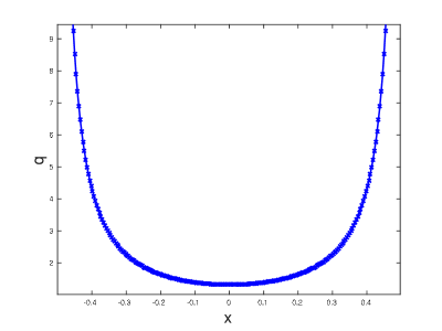
Figure 1: The analogous safety factor profile in region $x\in\left[-0.5,0.5\right]$ for initial background magnetic field, with $X=2$, $Y=4$, $Z=20$, $B_{0}=10$ and $B_{y0}\left(0\right)=1.5$. The safety factor tends to infinity near $x=\pm 0.5$ due to $B_{y0}$ being zero there.

As the turbulence grows in strength, it will have a back-reaction on the mean background field, leading to self-consistent evolution of the latter. The mean current profile will tend to relax under turbulence spreading Diamond1984 ; Strauss1986 ; Craddock1991 , and it is observed that substantial profile flattening would occur over time after the turbulence has been fully established. Ultimately, the relaxation would reach a point where there is no free energy available, and the tearing turbulence would then gradually decay away. However, it will be shown in Section IV.1 that the characteristic time scale of such decay is much longer than the slowest nonlinear turnover time of eddies, thus the turbulence can be viewed as having attained a quasi-steady-state before decay occurs.

III Analytical model for tearing turbulence

The structure of tearing turbulence spectrum will be discussed analytically in this section. Three quantities are needed in order to obtain the spectrum of tearing turbulence in a sheared guide field. The first is the effective damping rate caused by small-scale linearly stable modes, the second is the anisotropy property of the tearing turbulence, and the third is the local energy transfer in the $k$ space FrischBook ; DiamondBook . We will treat the effective damping and anisotropy property in Section III.1 and III.2 respectively, then substitute these results into the local energy transfer equation in Section III.3 to obtain the turbulence spectrum. In Section III.1, we will first justify the use of linear stability theory in considering the effective damping, then provide the $k_{\bot}$ scaling of growth rate and further obtain the effective damping rate for inviscid and viscous limit in Eq. (21)-(23). In Section III.2, we will investigate the scale-dependence of turbulence anisotropy by considering the ratio between the parallel wave number dispersion $\Delta k_{\|}\sim l_{\|}^{-1}$ as defined in Eq. (26) and the perpendicular wave number $k_{\bot}\sim l_{\bot}^{-1}$. The result is given in Eq. (34) and Eq. (40) for unperturbed and perturbed sheared guide field respectively. Finally, in Section III.3, we combine the aforementioned results with the local energy budget in Eq. (41) and the forward energy transfer rate in Eq. (44) to obtain the spectrum shape shown in Eq. (46).

III.1 Effective damping caused by linearly stable modes

We consider the effective damping under the assumption of weak nonlinearity, that is, the nonlinear interaction is assumed to be sufficiently weak that it does not change the linear outer region solution. Hence, we can still use linear theory to consider the mode structure, and the effective damping rate can be estimated from the negative linear growth rate.

The justification of using the linear growth rate to estimate effective damping may be formulated more precisely as follows. The effective island width $w$ for a given Fourier component of the magnetic perturbation ${\tilde{B}}_{k}\left(x,y,z\right)={\tilde{B}}_{k}^{(0)}\left(x\right)\exp{\left(ik_{y}y-ik_{z}z\right)}$ has the following dependence on mode numbers and the magnetic perturbation strength: WhiteRMP ; Di2015

$$w\sim\left(-\psi/\Psi_{0s}^{\prime\prime}\right)^{1/2}\sim\left(\frac{{\tilde{B}}_{x}}{B_{z0}}\frac{L_{s}}{k_{y}}\right)^{1/2},$$ (9)

where $\psi$ is the perturbed oblique flux

$$\psi\equiv{\tilde{A}}\cdot\vec{h},\quad\vec{h}\equiv\vec{e}_{z}+\left(k_{z}/k_{y}\right)\vec{e}_{y}.$$ (10)

Here, $\vec{h}$ is the oblique direction defined by given $k_{y}$ and $k_{z}$. Also, ${\tilde{B}}_{x}$ is the $x$ component of the corresponding magnetic perturbation and $\Psi_{0s}^{\prime\prime}$ is the second order derivative of background oblique flux taken at the resonant surface. Furthermore, $L_{s}\equiv Zq/s$ is the magnetic shear length and $s\equiv Yq^{\prime}/q$ is the magnetic shear. In the inviscid limit, the tearing layer width scales as Rutherford1973 ; Coppi1966 ; Glasser1975

$$x_{\eta}\sim\left(\frac{\eta}{v_{A}}\frac{L_{s}}{k_{y}}\right)^{2/5}\left(\Delta^{\prime}\right)^{1/5},$$ (11)

where $\Delta^{\prime}\equiv\psi_{s}^{\prime}/\psi_{s}\big{|}_{-}^{+}$ is the tearing stability index; the minus and plus signs here denote the left and the right side of the resonant surface. Alternatively, in the viscous regime we have Finn2005

$$x_{\eta}\sim\left(\frac{\eta}{v_{A}}\frac{L_{s}}{k_{y}}\right)^{1/3}P_{m}^{1/6},$$ (12)

where the magnetic Prandtl number $P_{m}\equiv\nu/\eta$. The following two factors justify the use of linear stability analysis. First, the perturbation amplitudes of high-$k$ modes are orders of magnitude smaller than that of low $k$ modes, thus the effective width of a high-$k$ island will also be much smaller than that of a low-$k$ island. Second, the effective island width will shrink faster than the tearing layer width for increasing $k$, as the power dependence on $k$ for the former is greater than that of the latter. Simple estimation using the turbulence spectrum obtained later in Section IV indicates that, in our case of weak turbulence, the island width will be smaller than the tearing layer width when $k_{\bot}\geq 25$. Furthermore, the contribution from hyper-resistivity is also ignored since it is proportional to the driven mode width to the fourth power, making its contribution less important for very small-scale modes. Craddock1991

We now examine the linear growth rate of the small-scale modes. The ideal linear eigen-equation for slab geometry can be written as Furth1963 ; BiskampBook ; Baalrud2012 :

$$\partial_{x}^{2}\psi=\left(k^{2}+\frac{F^{\prime\prime}}{F}\right)\psi.$$ (13)

Here, $F\equiv{\bf B}_{0}\cdot{\bf k}$, and $k$ is the wave number perpendicular to the oblique direction $\vec{h}$. It should be noted that we have $k_{\bot}\simeq k$ due to $k_{\|}\ll k_{\bot}$ as a result of the localized small-scale mode structure. For straight tearing modes with $k_{z}=0$, $F^{\prime\prime}/F$ remains finite even at the resonant surface where $F=0$. If $k_{\bot}^{2}\gg F^{\prime\prime}/F$, then the eigen-structure has the following form near resonant surface $x=x_{s}$:

$$\psi\simeq\psi_{s}\exp{\left(-k_{\bot}\left|x-x_{s}\right|\right)}.$$ (14)

Hence, for high $k$ modes which are linearly stable, we have:

$$\Delta^{\prime}\equiv\frac{\psi_{s}^{\prime}}{\psi_{s}}\Big{|}_{-}^{+}\simeq-2k_{\bot}.$$ (15)

For oblique modes, there is a logarithmic singularity in the derivative of the ideal solution since $F^{\prime\prime}/F$ is singular near the resonant surface Furth1963 ; Di2015 . However, the contribution of this logarithmic singularity to $\psi^{\prime}$ is even in parity near the resonant surface, thus does not contribute to $\Delta^{\prime}$. Hence, the $\Delta^{\prime}$ of high-$k$ oblique modes should have the same form as that of straight modes as shown in Eq. (15). Numerical solution of Eq. (13) confirms this statement Baalrud2012 .

The linear growth rate for oblique tearing modes in the inviscid limit is given by BiskampBook ; Baalrud2012

$$\gamma=\eta^{3/5}\left(\Delta^{\prime}\right)^{4/5}\left(k_{\bot}B_{ys}^{\prime}\right)^{2/5}\rho^{-1/5},$$ (16)

while in the viscous regime we have Finn2005

$$\gamma=\eta^{2/3}P_{m}^{-1/6}\Delta^{\prime}\left(k_{\bot}B_{ys}^{\prime}\right)^{1/3}\rho^{-1/6}.$$ (17)

Here, $B_{ys}^{\prime}$ is the $x$ gradient of $B_{y}$ taken at resonance $x_{s}$. The stable eigenmodes satisfying these dispersion relations are similar in mode structure and parity to the unstable modes that drive the turbulence. Equations (16) and (17) give the following $k_{\bot}$ dependence for $\gamma$:

$$\gamma\propto-\eta^{3/5}k_{\bot}^{6/5}$$ (18)

in the inviscid limit and

$$\gamma\propto-\eta^{2/3}P_{m}^{-1/6}k_{\bot}^{4/3}$$ (19)

in the viscous regime.

As has been mentioned in Section II, the background magnetic field is constantly evolving throughout the time-evolution of turbulence, hence we need to track the evolution of $B_{ys}^{\prime}$ numerically as the turbulence evolves. We define the following characteristic length scale of $B_{y}$ variation:

$$\lambda\equiv\frac{B_{y0}\left(0\right)}{B_{ys}^{\prime}.}$$ (20)

Thus, the effective damping in $k$ space can be written as:

$$\left[\partial_{t}E\left(k\right)\right]_{damping}=2\gamma E\left(k\right)=-2DS^{-p/2}\left(k_{\bot}\lambda\right)^{p}E\left(k\right),$$ (21)

with $p=6/5$ in the inviscid limit and $p=4/3$ in the viscous limit. Here, $E\left(k_{\bot}\right)=v\left(k_{\bot}\right)^{2}/k_{\bot}$ is the “energy density” in $k_{\bot}$ space. We consider a priori the equipartition of magnetic and kinetic energy for medium to high $k_{\bot}$. (We will check the validity of this assumption a posteriori). The Lundquist number $S$ is defined as $S\equiv\tau^{*}_{\eta}/\tau_{A}$, with $\tau^{*}_{\eta}\equiv\lambda^{2}/\eta$ and $\tau_{A}\equiv Z/v_{A}$, while $v_{A}$ is the Alfvén speed corresponding to the guide field. Furthermore, $D$ is the effective damping coefficient with dimension of $1/t$. Combining Eq. (16) or Eq. (17) with Eq. (21), we obtain

$$D=1.41\left(\frac{Z}{\lambda}\right)^{2/5}\left(\frac{B_{y0}}{B_{z0}}\right)^{2/5}\tau_{A}^{-1}$$ (22)

in the inviscid limit and

$$D=2\left(\frac{Z}{\lambda}\right)^{1/3}\left(\frac{B_{y0}}{B_{z0}}\right)^{1/3}\tau_{A}^{-1}P_{m}^{-1/6}$$ (23)

in the viscous regime. The damping rate given in Eq.(̇21) has a weaker dependence on $k_{\bot}$ than the classical dissipation does, making the distinction between the inertial range and the dissipation range hard to define. Thus, the present physical situation, in which damping appears to be important at all scales, does not permit a strict delineation of an inertial range in tearing turbulence.

III.2 Scale-independent anisotropy in sheared background field

The scale dependence of the ratio between the parallel and the perpendicular length scales of eddies is of great interest since it directly affects the nonlinear turnover rate and thus further influences the forward energy cascade rate of turbulence. The nonlinear turnover rate for MHD turbulence can be modeled as DiamondBook :

$$\frac{1}{\tau_{nl}}\simeq\frac{v\left(k_{\bot}\right)^{2}}{l_{\bot}^{2}}\frac{l_{\|}}{v_{A}}.$$ (24)

Here, $v\left(k_{\bot}\right)$ represents kinetic perturbation at $k_{\bot}$ scale.

For weak turbulence generated by oppositely propagating Alfvén waves with straight background field lines, the three-wave interaction preserves the $k_{\|}$ space structure of the beating waves, thus preventing any energy cascade along the direction parallel to the background magnetic field Ng96ApJ ; Ng96POP . A simple way to see this is by considering the resonant condition of wave number and frequency for three-wave interaction Shebalin1983 ; Sridhar2010 . We have:

$${\bf k}_{1}+{\bf k}_{2}={\bf k}_{3},\quad\omega^{\pm}_{1}+\omega^{\mp}_{2}=\omega^{\pm}_{3}.$$ (25)

Here, $\omega^{+}=v_{A}k_{\|}$ and $\omega^{-}=-v_{A}k_{\|}$ represent the angular frequencies of the forward and the backward propagating Alfvén waves, respectively. The oppositely propagating waves indicate that either $k_{1\|}$ or $k_{2\|}$ must be zero to satisfy both resonance conditions for the wave number and the frequency. Hence, there is no cascade of energy along $k_{\|}$ and the nonlinear turnover rate scales as $\tau_{nl}\propto v\left(k_{\bot}\right)^{2}l_{\bot}^{-2}$ as a result.

On the other hand, for a spectrum of modes in a sheared guide field, the parallel length scale $l_{\|}\simeq 1/\Delta k_{\|}$, where $\Delta k_{\|}$ is the dispersion in parallel wave number, and perpendicular length scale $l_{\bot}\simeq 1/k_{\bot}$, where $k_{\bot}$ is the perpendicular wave number. The dispersion in parallel wave number, $\Delta k_{\|}$, is defined as

$$\left(\Delta k_{\|}\right)^{2}\equiv\left<k_{\|}^{2}\right>_{k_{\bot},x}-\left<k_{\|}\right>^{2}_{k_{\bot},x}.$$ (26)

Here, $\left<f\right>_{k_{\bot},x}$ represents averaging quantity $f$ over $k_{\|}$ for a given $k_{\bot}$ and across the $\left(y,z\right)$ plane for a given $x$. Averaging over the $\left(y,z\right)$ plane is necessary because the small-scale mode structures are very localized and we are looking at the spectrum at a specific $x$. Within the framework of weak turbulence theory in a strong guide field where the average field is assumed to be unperturbed, we will find a similar independence between $l_{\|}$ and $l_{\bot}$ in the turbulence spectrum, i.e., $\Delta k_{\|}\propto k_{\bot}^{0}$, although the physical mechanism is somewhat different from that described above. However, it can be seen that the inclusion of a finite large-scale perturbation will introduce an additional relationship between $\Delta k_{\|}$ and $k_{\bot}$ in the spectrum, so long as we have ${\tilde{B}}_{L}L_{s}k_{\bot}/B_{z0}\gg 1$, where ${\tilde{B}}_{L}$ is the random large-scale perturbation, $L_{s}$ is the shear length of background guide field, and $B_{z0}$ is the guide field along the ignorable direction. It is important to note that $k_{\bot}$ in this criterion is the perpendicular wave number of the small-scale modes rather than the large-scale perturbation. Thus, the left-hand-side of the aforementioned criterion should not be confused with the Kubo number of the large-scale perturbation, defined as the ratio between the nonlinear and linear terms $\kappa\equiv\left({\tilde{B}}/B_{0}\right)/\left(l_{\|}/l_{\bot}\right)$.

We assume the perturbation has the following form: ${\tilde{B}}_{k}\left(x,y,z\right)={\tilde{B}}_{k}^{(0)}\left(x\right)\exp{\left(ik_{y}y-ik_{z}z\right)}$, where $m\equiv Yk_{y}/2\pi$ and $n\equiv Zk_{z}/2\pi$. For the unperturbed background field, we have:

$$k_{\|}=2\pi\left(\frac{B_{y0}}{B_{0}}\frac{m}{Y}-\frac{B_{z0}}{B_{0}}\frac{n}{Z}\right)=k_{y}\frac{Y}{Z}\frac{B_{z0}}{B_{0}}\left(\mu-\frac{n}{m}\right)=-\frac{k_{y}\Delta x}{L_{s}}\frac{B_{z0}}{B_{0}},\quad\mu\equiv 1/q.$$ (27)

Again, $L_{s}\equiv Zq/s$, $q\equiv YB_{z0}/ZB_{y0}$, and $s\equiv Yq^{\prime}/q$. We repeat for emphasis that $B_{y0}$ and $B_{z0}$ here do not contain the contribution of large-scale perturbation. The length $\Delta x\equiv x-x_{s}$ represents the distance to the resonant surface for a given $m/n$.

It will be shown later on in Section IV.1 that the characteristic length scale of turbulence strength envelope is much larger than $1/k_{\bot}$ in cases we are interested in, thus $\psi_{s}$ can be assumed to be independent of $\Delta x$ for a given $x$. Then Eq. (14) yields

$$\left<f\right>_{k_{\bot},x}=\left<\frac{\int_{-\infty}^{\infty}{\exp{\left(-2k_{\bot}\left|\Delta x\right|\right)}fd\Delta x}}{\int_{-\infty}^{\infty}{\exp{\left(-2k_{\bot}\left|\Delta x\right|\right)}d\Delta x}}\right>_{x}.$$ (28)

Note that here we integrate over $\Delta x$ instead of $k_{\|}$ because $dk_{\|}\propto d\Delta x$ so long as $k_{y}\propto k_{\bot}$. For the denominator, we have:

$$\int_{-\infty}^{\infty}{\exp{\left(-2k_{\bot}\left|\Delta x\right|\right)}d\Delta x}=\frac{e^{2k_{\bot}\Delta x}}{2k_{\bot}}\Big{|}_{-\infty}^{0}-\frac{e^{-2k_{\bot}\Delta x}}{2k_{\bot}}\Big{|}_{0}^{\infty}=\frac{1}{k_{\bot}}.$$ (29)

Thus we obtain:

$$\left<k_{\|}\right>_{k_{\bot}}=0,\quad\left(\Delta k_{\|}\right)^{2}=k_{\bot}\int_{-\infty}^{\infty}{\exp{\left(-2k_{\bot}\left|\Delta x\right|\right)}\left(\frac{k_{y}\Delta x}{L_{s}}\frac{B_{z0}}{B_{0}}\right)^{2}d\Delta x}.$$ (30)

Because the localized mode structure also implies that all the small-scale modes which can be “seen” from $x$ have similar $\mu$, we can approximately write:

$$k_{\bot}=\frac{B_{z0}}{B_{0}}k_{y}+\frac{B_{y0}}{B_{0}}k_{z},$$ (31)

$$\frac{Zk_{z}}{Yk_{y}}\simeq\mu\left(x\right).$$ (32)

Therefore, we obtain

$$k_{y}\simeq\frac{Z^{2}}{Z^{2}+Y^{2}\mu\left(x\right)^{2}}\frac{B_{0}}{B_{z0}}k_{\bot}.$$ (33)

Substituting the above relationship into Eq. (30), the parallel length scale $l_{\|}$ for small scale perturbations is found to be independent of $k_{\bot}$

$$l_{\|}^{-2}=\left(\Delta k_{\|}\right)^{2}\simeq\frac{Z^{2}}{Z^{2}+Y^{2}\mu\left(x\right)^{2}}\frac{1}{2L_{s}^{2}}\propto k_{\bot}^{0}.$$ (34)

This is similar to the weak turbulence limit discussed in Ref. [Ng96ApJ, ] and Ref. [Ng96POP, ], although the underlying physics is quite different.

Now, let us consider the effect of a large-scale perturbation on the small-scale anisotropy. We consider the summation of several large-scale modes as a random magnetic perturbation strong enough to twist the field “seen” by the small-scale modes. Let ${\tilde{B}}_{L}$ be the perturbation component in $\left(y,z\right)$ plane. Thus, the parallel wave number for each mode is now:

$$k_{\|}=-\frac{k_{y}\Delta x}{L_{s}}\frac{B_{z0}}{B_{0}}+\frac{{\tilde{B}}_{Ly}}{B_{0}}k_{y}-\frac{{\tilde{B}}_{Lz}}{B_{0}}k_{z}.$$ (35)

Recalling Eq. (32), for given $x$, we have:

$$k_{\|}\simeq-\frac{B_{z0}}{B_{0}}\frac{k_{y}\Delta x}{L_{s}}+\frac{{\tilde{B}}_{Ly}}{B_{0}}\left[1-\frac{Y}{Z}\mu\left(x\right)\frac{{\tilde{B}}_{Lz}}{{\tilde{B}}_{Ly}}\right]k_{y}.$$ (36)

For simplicity, we define the following parameters:

$$T\equiv\frac{B_{z0}}{B_{0}},\quad U\equiv\frac{{\tilde{B}}_{Ly}}{B_{0}}\left[1-\frac{Y}{Z}\mu\left(x\right)\frac{{\tilde{B}}_{Lz}}{{\tilde{B}}_{Ly}}\right].$$ (37)

An important feature of the latter parameter is that the contribution from the large-scale perturbation vanishes upon taking the $\left(y,z\right)$ plane average since $U$ vanishes under such spatial average, although $U^{2}$ does not.

Carrying out the same method used above, we also obtain

$$\left<k_{\|}\right>_{k_{\bot},x}=\left<U\frac{B_{0}}{B_{z0}}k_{\bot}\right>_{x}=0,$$ (38)

as well as

$$\left<k_{\|}^{2}\right>_{k_{\bot},x} \simeq \left<k_{\bot}\frac{B_{0}^{2}}{B_{z0}^{2}}\int_{-\infty}^{\infty}{e^{-2k_{\bot}\Delta x}\left[T^{2}\left(\frac{k_{\bot}}{L_{s}}\right)^{2}\Delta x^{2}-2TU\frac{k_{\bot}^{2}}{L_{s}}\Delta x+U^{2}k_{\bot}^{2}\right]d\Delta x}\right>_{x}$$ (39)

$$= \left<\frac{B_{0}^{2}}{B_{z0}^{2}}\left(\frac{T^{2}}{2L_{s}^{2}}+U^{2}k_{\bot}^{2}\right)\right>_{x}.$$

Thus, so long as $2U^{2}k_{\bot}^{2}L_{s}^{2}/T^{2}\gg 1$, we have

$$\Delta k_{\|}=\sqrt{\left<\frac{B_{0}^{2}}{B_{z0}^{2}}\left(\frac{T^{2}}{2L_{s}^{2}}+U^{2}k_{\bot}^{2}\right)\right>_{x}}\simeq\frac{B_{0}}{B_{z0}}\sqrt{\left<U^{2}\right>_{x}}k_{\bot}\propto k_{\bot},$$ (40)

resulting in a scale-independent anisotropy $l_{\|}/l_{\bot}\propto l_{\bot}^{0}$. Here, we emphasize that $U/T$ can still be small for the condition $2U^{2}k_{\bot}^{2}L_{s}^{2}/T^{2}\gg 1$ to be valid due to the largeness of $L_{s}k_{\bot}$, with $k_{\bot}$ being the wave number of small-scale modes.

III.3 Local energy budget in $k_{\bot}$ space

The impact of non-negligible dissipation on the structure of the spectrum has been studied by considering the local energy budget in the $k$ space Terry2009 ; Terry2012 . We will follow this methodology here, albeit in the context of turbulence with scale-independent anisotropy instead of turbulence that is critically balanced one, as discussed in Section III.2.

Under the local interaction assumption, the local energy budget in the $k_{\bot}$-space naturally arises from considerations of the effective damping and classical resistive diffusion, Terry2009 ; Terry2012 :

$$-2DS^{-p/2}\left(k_{\bot}\lambda\right)^{p}E\left(k_{\bot}\right)-2\tau_{\eta}^{*-1}\left(k_{\bot}\lambda\right)^{2}E\left(k_{\bot}\right)=\frac{dT\left(k_{\bot}\right)}{dk_{\bot}},$$ (41)

where $\tau_{\eta}^{*}\equiv\lambda^{2}/\eta$, $T\left(k_{\bot}\right)$ is the energy forward transfer rate at scale $k_{\bot}$, and $E\left(k_{\bot}\right)=v\left(k_{\bot}\right)^{2}/k_{\bot}$ is the energy density in the $k_{\bot}$ space. The energy budget Eq. (41) can be solved to yield the energy spectrum if $T\left(k_{\bot}\right)$ can be written as a function of $E\left(k_{\bot}\right)$. The traditional scaling for MHD turbulence without scale-dependent alignment indicates that DiamondBook

$$T\left(k_{\bot}\right)=\frac{v\left(k_{\bot}\right)^{2}}{\tau_{nl}}\simeq\frac{v\left(k_{\bot}\right)^{4}}{l_{\bot}^{2}}\frac{l_{\|}}{v_{A}}.$$ (42)

Here, $v\left(k_{\bot}\right)$ represents the kinetic perturbation at $k_{\bot}$ scale, and $v_{A}$ is the Alfvén speed measured with the guide field. Due to the equipartition of kinetic and magnetic energy, $T\left(k_{\bot}\right)$ also represents the forward cascade of magnetic energy as $v\left(k_{\bot}\right)=v_{A}\left({\tilde{B}}\left(k_{\bot}\right)/B_{0}\right)$ with ${\tilde{B}}\left(k_{\bot}\right)$ as the magnetic perturbation at $k_{\bot}$ scale.

Using the scale-independent anisotropy discussed before, the forward transfer rate is now

$$T\left(k_{\bot}\right)=\frac{v\left(k_{\bot}\right)^{4}}{l_{\bot}\alpha v_{A}},\quad\alpha\equiv\frac{l_{\bot}}{l_{\|}}.$$ (43)

Here, $\alpha$ is a constant characterizing the scale-independent anisotropy, the value of which will be extracted from numerical simulations of tearing turbulence. We follow the closure technique used in Refs. [Terry2009, ] -  [TLBook, ], and write the forward energy transfer rate

$$T\left(k_{\bot}\right)\, =\, v\left(k_{\bot}\right)^{4}k_{\bot}\left(\alpha v_{A}\right)^{-1}$$ (44)

$$= E\left(k_{\bot}\right)k_{\bot}^{2}\left(\alpha v_{A}\right)^{-1}v\left(k_{\bot}\right)^{2}$$

$$= E\left(k_{\bot}\right)\epsilon^{1/2}k_{\bot}^{3/2}\left(\alpha v_{A}\right)^{-1/2}.$$

Here, we have used the closure $v\left(k_{\bot}\right)^{2}\simeq\epsilon^{1/2}k_{\bot}^{-1/2}\left(\alpha v_{A}\right)^{1/2}$. This closure technique effectively builds the inertial power-law behavior into the energy spectrum as an asymptote in the low-damping limit. Therefore, as can be seen later in this section, the spectrum approaches a simple power law when the effective damping vanishes.

Substituting Eq. (44) into Eq. (41), we obtain a linear first order ordinary differential equation for the energy spectrum:

$$\frac{d}{dk_{\bot}}E\left(k_{\bot}\right)k_{\bot}=-\frac{3}{2}E\left(k_{\bot}\right)-\left[2DS^{-p/2}\left(k_{\bot}\lambda\right)^{p-1/2}+2\tau_{\eta}^{*-1}\left(k_{\bot}\lambda\right)^{3/2}\right]$$

$$\times E\left(k_{\bot}\right)\epsilon^{-1/2}\left(\alpha v_{A}\right)^{1/2}\lambda^{1/2}.$$ (45)

The tearing turbulence spectrum with linear stabilities act as effective damping is then:

$$E\left(k_{\bot}\right)\, \sim\, \left(\alpha v_{A}\right)^{1/2}\epsilon^{1/2}k_{\bot}^{-3/2}\exp{\left[-2DS^{-p/2}\frac{\epsilon^{-1/2}\lambda^{1/2}\left(\alpha v_{A}\right)^{1/2}}{p-\frac{1}{2}}\left(k_{\bot}\lambda\right)^{p-1/2}\right]}$$ (46)

$$\times\exp{\left[-2\tau_{\eta}^{*}\frac{\epsilon^{-1/2}\lambda^{1/2}\left(\alpha v_{A}\right)^{1/2}}{3/2}\left(k_{\bot}\lambda\right)^{3/2}\right]},$$

with $p=6/5$ and $p=4/3$ in the inviscid and viscous regime respectively, while effective damping coefficient $D$ is given by Eq. (22) and Eq. (23). From Eq. (46), it can be seen that the primary impact of effective damping is an exponential multiplier on the original power law. In the limit of small effective damping, the spectrum recovers the simple power-law behavior predicted by the assumption of an inertial range. Also, the power-law behavior in the no damping limit tends to be $k_{\bot}^{-3/2}$ due to the scale independent anisotropy $l_{\|}\propto l_{\bot}$.

IV Simulations

In this section, the analytical result from Section III will be tested against resistive MHD simulation using the same set of equations (1) - (4) described in Section II. Specifically,we are concerned with the structure of the energy spectrum $E\left(k_{\bot}\right)$ and the dependence of $k_{\bot}/k_{\|}$ on $k_{\bot}$. We will first examine the strong guide field case where $B_{y0}/B_{z0}\sim\mathcal{O}\left(10^{-1}\right)$ and ${\tilde{B}}_{L}/B_{z0}\sim\mathcal{O}\left(10^{-2}\right)$. We will then consider the case of comparable guide field where $B_{y0}/B_{z0}\sim\mathcal{O}\left(1\right)$ and the large-scale perturbed field is only one order of magnitude smaller than the guide field ${\tilde{B}}_{L}/B_{z0}\sim\mathcal{O}\left(10^{-1}\right)$. In the latter case, the Kubo number for the large-scale perturbation is $\kappa=\left({\tilde{B}}_{L}/B_{0}\right)\left(L_{\|}/L_{\bot}\right)\geq 1$, corresponding to the regime where turbulent shearing is comparable with parallel propagation. Here, the Kubo number $\kappa$ is equivalent to the $\chi$ used by Goldreich and Sridhar in Ref. [GS1997, ]. Numerical observation of the magnetic shear length indicates we have $2{\tilde{B}}_{L}^{2}L_{s}^{2}k_{\bot}^{2}/B_{z0}^{2}>\mathcal{O}\left(10^{2}\right)$ when $k_{\bot}>20$ for both of the above cases. The numerical algorithm will follow that of Ref. [Huang16APJ, ] and Ref. [Guzdar1993, ]. Five-point finite difference scheme is used to calculate derivatives, and trapezoidal leapfrog is used for time stepping scheme. The resistivity is set to be $\eta=1\times 10^{-4}$, and the magnetic Prandtl number is $P_{m}\equiv\nu/\eta=1$, and thus we are in the viscous regime discussed above. In the numerical scheme, an additional artificial fourth-order dissipation is also implemented to damp small-scale fluctuations at grid size. This should not be confused with the real hyper-dissipation self-consistently generated by the nonlinear terms Strauss1986 ; Craddock1991 .

IV.1 Strong guide field case

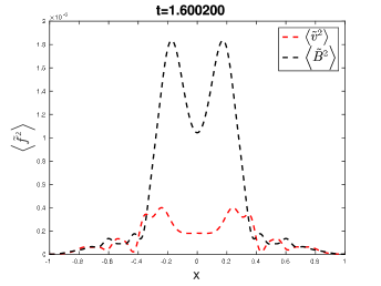
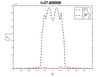
(a)	(b)
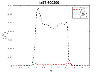
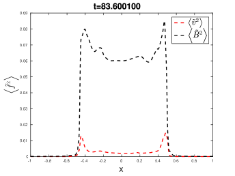
(c)	(d)

Figure 2: The perturbed energy profile for different times. Most of the perturbed energy locates within $x\in\left[-0.5,0.5\right]$. At the beginning of the simulation, only a few large-scale unstable tearing modes exist, and the envelope of their mode structures defines the perturbed energy profile. As time goes on, these large-scale modes overlap with each other and generate the tearing turbulence, flattening the perturbed energy profile.

In this subsection, we will compare the tearing turbulence in a strong guide field with our previous theoretical model. Let $X=2$. $Y=4$, $Z=20$, $B_{y0}\left(0\right)=1.5$ and $B_{0}=10$.

At the beginning of the simulation, small initial perturbations with harmonics $m/n=3/2$, $2/1$ and $3/1$ are seeded. The resonant surfaces corresponding to those modes lie in the central region of the system $x\in\left[-0.5,0.5\right]$, as can be seen from Fig. 1. This is also the region where the turbulence amplitude is strongest later in time. The quadratic form of magnetic and kinetic perturbation is averaged across the $y$-$z$ plane, providing us the sum of perturbation energy over the whole spectrum, $\left<{\tilde{v}}^{2}\right>$ and $\left<{\tilde{B}}^{2}\right>$, given by

$$\left<{\tilde{B}}^{2}\right>=\left<B^{2}\right>-\left<B\right>^{2},$$ (47)

$$\left<{\tilde{v}}^{2}\right>=\left<v^{2}\right>-\left<v\right>^{2}.$$ (48)

These perturbation energies as functions of $x$ are plotted in Fig. 2 for different times. Initially, the dynamics is dominated by a few large-scale unstable modes, and the envelope of their mode structure determines the perturbation energy profile, as can be seen from Fig. 2 (a) and Fig. 2 (b). Later, the initial islands overlap with each other and generate a large spectrum of small-scale modes, and the perturbation energy profile becomes smooth in the core region, as seen in Fig. 2 (c) and Fig. 2 (d). By the time the tearing turbulence enters quasi-steady state, both the magnetic and kinetic energy perturbations are confined within the region $x\in\left[-0.5,0.5\right]$, and their profiles are almost flattened within the central region. The kinetic perturbation seems to be much smaller than the magnetic perturbation, which would appear to raise doubt regarding our energy equipartition assumption. However, as will be seen later in Section IV.1, this is because equipartition is established not at the scale of the large-scale instabilities driving the turbulence but at the small scales. Meanwhile, the spectrum for high-$k$ modes actually agrees rather well with the equipartition assumption.

The alignment of the turbulent eddies to the local mean field is also of interest. That is, we wish to know whether or not the eddies have elongated structure along the mean field direction, as would be expected from highly magnetized MHD turbulence. Here, we look at the local property of magnetic perturbation for a given $x$ position, and perform Fourier decomposition along $y$ and $z$ direction for all components of magnetic field. We take the zeroth order harmonic as the local mean field for the given $x$ position, while all the other harmonics correspond to modes with various scales. The alignment of those modes to the direction of local mean field line can be represented by looking at ${\bf k}\cdot{\bf B}_{0}$. We once again write

$${\bf k}\cdot{\bf B}_{0}=B_{y0}k_{y}-B_{z0}k_{z}=k_{y}\frac{Y}{Z}\left(\mu-\frac{n}{m}\right)B_{z0}.$$ (49)

Such alignment of small-scale tearing modes can then be checked by looking at the distribution of the 2-D perturbed energy spectrum $\left|{\tilde{B}}_{k}\right|^{2}$ and $\left|{\tilde{v}}_{k}\right|^{2}$ in $\left(m,n\right)$ space. The result for $x=0$ is shown in Fig. 3, where the logarithm of the perturbed energy is plotted as a function of mode number $m$ and $n$. The black dashed line represents the contour of ${\bf k}\cdot{\bf B}_{0}$, with the one originating from the $\left(0,0\right)$ point corresponding to ${\bf k}\cdot{\bf B}_{0}=0$. It can be seen that the energy spectrum strongly aligns with the local mean field, indicating a strongly anisotropic structure. It is noteworthy that, for a magnetically sheared system, this localization in the $k$ space directly corresponds to the localization of mode structures near their respective resonant surfaces in configuration space. Due to this localized mode structure, the amplitude of the mode decreases rapidly as we move away from its resonant surface. Thus, only modes which are near resonance (corresponds to low $k_{\|}$) can be seen from the spectrum shown in Fig. 3, resulting in observed localization in the $k$ space. This is especially true for high-$k$ modes. The red dashed lines represent the contours of $k_{\bot}$. The strong alignment behavior of small-scale perturbation in the presence of strong guide field indicates that we have $k_{\|}\ll k_{\bot}$, and consequently $k_{y}^{2}+k_{z}^{2}=k_{\bot}^{2}+k_{\|}^{2}\simeq k_{\bot}^{2}$. This confirms our previous assumptions.

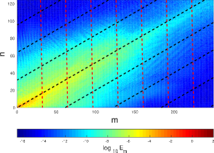
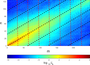
(a)	(b)

Figure 3: The alignment of turbulent eddies to local mean field line at $x=0$. The color here represents the logarithm of perturbed energy density of (a) magnetic perturbation, and (b) kinetic perturbation. The black dashed lines are the contours of ${\bf k}\cdot{\bf B}_{0}$. It can be seen that the turbulence is highly anisotropic, and tend to align with the direction of strong mean field. The red dashed lines represent the contours of $k_{\bot}$ in $\left(m,n\right)$ plane.

With the alignment of eddies known, we now look at how this highly anisotropic turbulence establishes itself. From Fig. 2 (c) and (d), it can be seen that the turbulence strength is rather flat in the central region, this implies that we can use the local spectrum for a given $x$ to represent the evolution of global tearing turbulence. Here, we choose to look at the spectrum evolution at $x=0$. The energy density in $k_{\bot}$ space $E\left(k_{\bot}\right)$ can be obtained by integrating over the red dashed lines in Fig. 3. The spectrum of $E\left(k_{\bot}\right)$ for several different times is presented in Fig. 4. The logarithm of magnetic energy perturbation is shown as a function of the logarithm of the perpendicular scale $k_{\bot}$. It can be seen that at $t=0$ there are only several large-scale unstable modes. Then the interaction of these large-scale modes gradually stir up small-scale modes. At a later time, the tearing turbulence reaches a quasi-steady state as can be seen in Fig. 4. The structure of $E\left(k_{\bot}\right)$ spectrum changes very little from $t=63.6$ to $t=109.6$ while the longest non-linear turnover time of the eddies is on the order of $\tau_{nl}\sim 1$.

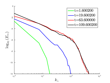
Figure 4: The time evolution of the tearing turbulence energy spectrum. At $t=0$, there are only several unstable modes. These large scale modes gradually excite a spectrum of small-scale modes by interacting with each other. At a later time, the tearing turbulence reaches a quasi-steady state.

The comparison between magnetic and kinetic energy spectrum after the turbulence reached the quasi-steady state is another important issue, as we have assumed an equipartition of energy in Section III.3. An example kinetic and magnetic spectrum for quasi-steady state tearing turbulence is shown in Fig. 5 for $t=85.6$. It can be seen that for high-$k$ modes the kinetic and magnetic energy are approximately the same, while at the largest scale there is a departure from equipartition. The departure does not significantly impact our theoretical analysis in Section III.3, since we are primarily concerned with small-scale modes which are linearly stable rather than the unstable large-scale modes. As a side note, the fact that the magnetic perturbation is one order of magnitude larger than the kinetic perturbation for largest scale modes is also consistent with the observation in Fig. 2, as the total magnetic perturbation energy is also one order of magnitude larger than the total kinetic perturbation energy.

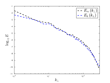
Figure 5: Comparison between kinetic and magnetic spectrum for $t=85.6$. It can be seen that the equipartition of energy is reasonably satisfied for high-$k_{\bot}$ modes, while there is some departure from equipartition for large-scale modes. The perturbed magnetic energy is approximately one order of magnitude larger than the kinetic energy for the largest mode.

The next important property we are interested in is the structure function of the turbulence, which provides us information regarding the scale dependence of its anisotropy and thus has significant impact on the energy transfer rate and consequently the turbulence spectrum. We follow the procedure detailed in Ref. [Huang16APJ, ] and Ref. [Cho2000, ], and define the following two-point structure functions:

$$F_{k}\left(l_{\|},l_{\bot}\right)\equiv\left<\left|{\bf v}\left({\bm{\zeta}}+{\bf l}\right)-{\bf v}\left({\bm{\zeta}}\right)\right|^{2}\right>,$$ (50)

$$F_{m}\left(l_{\|},l_{\bot}\right)\equiv\left<\left|{\bf B}\left({\bm{\zeta}}+{\bf l}\right)-{\bf B}\left({\bm{\zeta}}\right)\right|^{2}\right>.$$ (51)

Here, ${\bm{\zeta}}=\left(x,y,z\right)$ is the position of a random point in the configuration space, and ${\bf l}$ is a random vector. Thus, ${\bm{\zeta}}+{\bf l}$ and ${\bm{\zeta}}$ define a random pair of points in configuration space. The bracket $\left<f\right>$ here indicates an ensemble average over a large number of random pairs. Due to the strong localization of mode structure demonstrated in Fig. 3, we look at a 2D version of the structure function in our study. That is, we take the random pairs within the $y$-$z$ plane for a given $x$ instead of considering the full 3D space. The parallel and perpendicular component of ${\bf l}$ is defined by the local mean field direction, which is calculated by averaging the magnetic field at two points. We average over $10^{9}$ random pairs of points, and obtain the structure function for both kinetic and magnetic perturbation as functions of $l_{\|}$ and $l_{\bot}$. The contours of this structure function in $\left(l_{\|},l_{\bot}\right)$ then reflect the anisotropy of the eddy at different $l_{\bot}$ scales.

To extract this anisotropy information, we search for the intersection of a given contour of $F_{k}\left(l_{\|},l_{\bot}\right)$ or $F_{m}\left(l_{\|},l_{\bot}\right)$ with the $l_{\|}$ and $l_{\bot}$ axis respectively. Thus we can obtain a pair of $l_{\|}$ and $l_{\bot}$ for a given contour of $F_{k}\left(l_{\|},l_{\bot}\right)$ or $F_{m}\left(l_{\|},l_{\bot}\right)$, the ratio of which represents the anisotropy at a given scale. A scan of these $l_{\|}$ and $l_{\bot}$ pairs then shows the scale dependence of turbulence anisotropy. The anisotropy thus obtained is plotted in Fig. 6, with two scalings $k_{\|}\propto k_{\bot}$ and $k_{\|}\propto k_{\bot}^{2/3}$ plotted as black dashed lines. It can be seen that the anisotropic behavior of simulation result largely agrees with our analytical model and is mostly scale-independent. There is some discrepancy between the length scale of kinetic and magnetic perturbations, which might be the consequence of their different distribution width in $\left(k_{y},k_{z}\right)$ space as can be seen in Fig. 3. The ratio between parallel and perpendicular length scale ultimately deviates from the scale-independent scaling at the very small scale where classical dissipation kicks in. Lastly, it is observed that $l_{\|}$ is two orders of magnitude larger than $l_{\bot}$, thus we hereby take $\alpha\sim 10^{-2}$ as a reasonable estimation. This estimation also agrees with our prediction by Eq. (40) since we also have ${\tilde{B}}_{L}/B_{z0}\sim\mathcal{O}\left(10^{-2}\right)$.

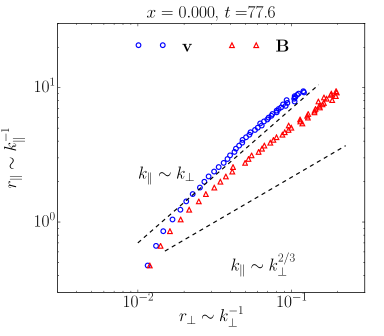
Figure 6: The anisotropy of tearing turbulence for various scale $l_{\bot}$. Both the kinetic and magnetic perturbation is shown. The scaling of both $k_{\|}\propto k_{\bot}$ and $k_{\|}\propto k_{\bot}^{2/3}$ are shown as black dashed lines. It can be seen that the turbulence anisotropy is scale independent $k_{\|}\propto k_{\bot}$ for most of the scales.

With the characteristic structure known, we can finally check our analytical model given by Eq. (46) against the simulation results. The magnetic perturbation spectrum for tearing turbulence is shown in Fig. 7 for $t=85.6$ and $x=0$. The simulation result is compared with three analytical models: our damped turbulence model as shown in Eq. (46), a simple power law $E\left(k_{\bot}\right)\propto k_{\bot}^{\beta}$ as a result of the traditional inertial range argument, and the spectrum produced by Eq. (46) if only the resistivity is included as damping. From numerical observation, we estimate the characteristic length scale to be $\lambda\simeq 10$ near the central flattened region where the resonant surfaces of the concerned modes lie. Here $\lambda$ can be larger than $X$ since it only serves as an indication of the local magnetic field gradient. The only free parameter in Eq. (46) is then the energy injection rate $\epsilon$, which will be used to fit the simulation result. On the other hand, the power index $\beta$ in the simple power law will also be used as a free parameter to fit the numerical result. The fitting exercise yields $\epsilon\simeq 1.2\times 10^{-3}$ and $\beta\simeq-2.0$, with fixed parameters $\lambda=10$ and $\alpha=0.01$. The fitted curves are shown in Fig. 7. It can be seen that our analytical model is in better agreement with the simulation result than either the simple power law or the spectrum obtained by assuming that it is determined by the effect of resistivity only. It is noteworthy that although the final decay of the turbulence spectrum is due to the influence of resistivity, the actual curve deviates from the inertial range curve due to the presence of effective damping. While this deviation might suggest that there exists an inertial range with a steeper slope represented, for instance, by the blue dashed line, this is not the case since the behavior seen is caused by slow exponential decay and cannot be represented accurately by a power law.

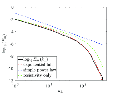
Figure 7: The spectrum of tearing turbulence for $t=85.6$ and $x=0$, compared with three analytical models. The black solid line represents the simulation result, the red dashed line is a fitting of Eq. (46) using only the energy injection rate $\epsilon$ as a free parameter, the blue dashed line corresponds to a simple power law $E_{m}\left(k_{\bot}\right)\propto k^{-2.0}$, and the green dashed line is the spectrum produced by Eq. (46) if we only consider the resistive damping. The simulation result agrees rather well with our analytical prediction.

IV.2 Weaker guide field case

The strong guide field case has been investigated in the previous subsection. Reasonable agreement has been found between the simulation result and our theoretical prediction obtained in Section III. The magnitude of the perturbation has been found to be two order of magnitude smaller than the guide field. However, we are also interested in cases where the guide field is weaker, and the large-scale Kubo number $\kappa=\left({\tilde{B}}_{L}/B_{0}\right)\left(L_{\|}/L_{\bot}\right)\simeq 1$. Again, $\kappa$ here is equivalent to the $\chi$ used in Ref. [GS1997, ]. Note that, in this case of stronger turbulence, the perturbed field is still smaller than the guide field, although the Kubo number may exceed unity due to anisotropy.

The initial magnetic fields are now $B_{y0}\left(0\right)=1.5$ and $B_{0}=2.5$. To maintain a similar initial safety factor profile with the one shown in Fig. 1, the system size is now $X=2$, $Y=4$ and $Z=4$. We are mainly concerned with the anisotropic behavior and the energy spectrum of the turbulence, and we wish to determine whether or not the distinctive features exhibited in our weak turbulence simulation persist in this stronger turbulence case.

We first examine the anisotropy. Again, we look at the contours of structure functions for both the kinetic and magnetic perturbation as described in Section IV.1, and we use the same technique detailed there to extract the turbulence anisotropy for different scales. The $x$ position is chosen at $x=0$, and time $t=59.6$, when the turbulence has already reached the quasi-steady state. The anisotropy is shown in Fig.8, with the two scalings $k_{\|}\propto k_{\bot}$ and $k_{\|}\propto k_{\bot}^{2/3}$ plotted as black dashed lines. It can be seen that this stronger turbulence case still follows the scale-independent anisotropy behavior described in Section III.2 and only deviates from it at very small scales. In fact, the scale-independent anisotropy is even better compared to that shown in Fig. 6, possibly due to a stronger large-scale perturbation.

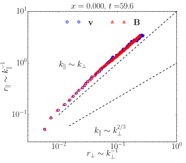
Figure 8: The scale-independent anisotropy for a weaker guide field case. Although the turbulence is now less anisotropic than in the strong guide field case, the fundamental scale-independent anisotropy remains the same comparing with what is shown in Fig. 6.

We then look at the structure of the turbulence spectrum. The magnetic perturbation spectrum for $x=0$ and $t=59.6$ is shown in Fig.9. Once again, the simulation result is compared with a simple power law $E\left(k_{\bot}\right)\propto k_{\bot}^{-2.4}$ and the spectral form predicted by our model as described by Eq. (46), with fixed parameters $\lambda=10$ and $\alpha=0.05$. The fitting result returns $\epsilon=8.5\times 10^{-4}$. Reasonable agreement is again found between the numerical result and our prediction, with a gradual departure from the original $k^{-3/2}$ scaling well before entering the resistive dissipation scale.

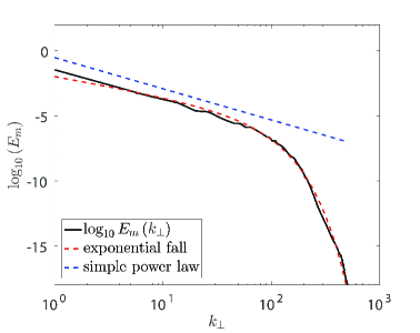
Figure 9: The spectrum of tearing turbulence for $t=59.6$ and $x=0$, compared with two analytical model. As is shown in Fig. 7, the simulation result agrees rather well with our analytical prediction, suggesting that our analytical model works well even for not-so-weak turbulence.

A noteworthy feature of this stronger turbulence case is that the Kubo numbers for the largest perturbations exceed unity. From Fig. 8, it can be seen that the scale-independent anisotropy is approximately $l_{\|}/l_{\bot}\simeq 20$. At the same time, numerical observation from Fig. 9 indicates the largest scale perturbation has ${\tilde{B}}_{L}/B_{0}\sim\mathcal{O}\left(10^{-1}\right)$. Hence, for the large-scale perturbations, we have $\kappa\simeq 2$, while for smaller scale perturbation the Kubo number steadily decreases as the perturbation strength decreases. This is different from the critical balance scenario where the Kubo number remains on the order of unity across all scales. This deviation from critical balance is very similar to that discussed by Huang et al. in Ref. [Huang16APJ, ]. Thus, we conclude that our analysis can also be applied to the case where the nonlinear mixing is stronger than the linear parallel propagation, such as those reported in plasmoid turbulence, where the critical balance condition was frequently assumed to be true.

V Discussion and conclusion

Instability driven tearing turbulence in sheared magnetic field is studied in this work. The turbulence consists of several large-scale unstable modes and a broad spectrum of small-scale linearly stable modes which are excited by their large-scale counterparts. It is found that the linearly stable modes will act as an effective damping mechanism which has a weaker dependence on $k_{\bot}$ than classical dissipation. For inviscid and viscous regimes, the dependence scales as $k_{\bot}^{6/5}$ and $k_{\bot}^{4/3}$ respectively. The weak dependence indicates that this damping mechanism will manifest itself long before turbulence eddies reach the resistive or viscous dissipation scales. Consequently, a well-defined inertial range cannot be identified, and damping must be considered at all scales. Furthermore, we argue that the tilting of sheared background field by large-scale perturbations will impose a scale-independent anisotropy for small-scale modes. This anisotropic behavior then determines the scale dependence of the forward energy cascade rate.

With the knowledge of effective damping rate and energy cascade rate at hand, the structure of this damped turbulence can be obtained by considering local energy budget in the $k_{\bot}$ space. The key idea is that the difference of energy forward transfer rate between the two ends of any interval in the $k_{\bot}$ space corresponds to the damping within that interval. The resulting spectrum features a power law multiplied by an exponential falloff, as opposed to the pure power-law spectrum obtained by using the standard inertial range argument.

The above analytical result is checked against visco-resistive MHD simulations. The turbulence is found to be highly anisotropic and tends to align with the strong local mean-field direction. The two-point structure functions are calculated to investigate anisotropic property at different scales, and a scale-independent anisotropy is found, confirming our $l_{\|}\propto l_{\bot}$ argument. Furthermore, the equipartition between kinetic and magnetic energy is found to be valid for the turbulence in question. The numerical result appears to agree well with our analytical model based on effective damping.

The behavior of a stronger turbulence, where the Kubo number exceeds unity for certain scales, is also investigated. We find that the scale-independent anisotropy and the energy spectrum continue to hold for the stronger turbulence case, indicating that our analysis remains applicable even for the scenario where the perpendicular turbulence shearing is stronger than the parallel propagation.

With this knowledge regarding spectrum structure, the next step would be considering the back-reaction of small-scale turbulence on large scales. This involves a sum of quadratic form of perturbed quantities over the whole spectrum, which requires knowledge regarding the form of spectrum given by our study here. An example is the small-scale spreading of mean field described by hyper-resistivity, as has been studied in Ref. [Strauss1986, ] and Ref. [Craddock1991, ]. Our analysis here provides a solid basis for future study along these lines. These studies are left to future work.

Acknowledgments

The authors thank P. H. Diamond, X.-G. Wang, H.-S. Xie and L. Shi for fruitful discussion. This work is partially supported by the National Natural Science Foundation of China under Grant No. 11261140326 and the China Scholarship Council. A. Bhattacharjee and Y.-M. Huang acknowledge support from NSF Grants AGS-1338944 and AGS-1460169, and DOE Grant DE-SC0016470. Simulations were performed with supercomputers at the National Energy Research Scientific Computing Center. D. Hu publishes this paper while working in ITER Organization. ITER is a Nuclear Facility INB-174. The views and opinions expressed herein do not necessarily reflect those of the ITER Organization.

References

- (1) H. A. B. Bodin, “The reversed field pinch”. Nucl. Fusion 30 1717 (1990);
- (2) P. H. Diamond, R. D. Hazeltine, Z. G. An, B. A. Carreras and H. R. Hicks, “Theory of anomalous tearing mode growth and the major tokamak disruption”. Phys. Fluids 27 1449 (1984);
- (3) H. R. Strauss, “Hyperresistivity produced by tearing mode turbulence”. Phys. Fluids 29 3668 (1986);
- (4) G. G. Craddock, “Hyperresistivity due to densely packed tearing mode turbulence”. Phys. Fluids B 3 316 (1991);
- (5) W. Daughton, V. Roytershteyn, H. Karimabadi, L. Yin, B. J. Albright, B. Bergen and K. J. Bowers, “Role of electron physics in the development of turbulent magnetic reconnection in collisionless plasmas”. Nature Physics 7 539-542 (2011);
- (6) Y.-M. Huang, A. Bhattacharjee, “Turbulent magnetohydrodynamic reconnection mediated by the plasmoid instability”. Ap. J. 818 20 (2016);
- (7) A. H. Boozer, “Ohm’s law for mean magnetic field”. J. Plasma Phys. 35 133-139 (1986);
- (8) A. Bhattacharjee, E. Hameiri, “Self-consistent dynamolike activity in turbulent plasma”. Phys. Rev. Lett. 57 206 (1986);
- (9) E. Hameiri, A. Bhattacharjee, “Turbulent magnetic diffusion and magnetic field reversal”. Phys. Fluids 30 1743 (1987);
- (10) U. Frisch, “Turbulence - The legacy of A. N. Kolmogorov”. (Cambridge University Press, Cambridge, 1995), p. 72;
- (11) P. H. Diamond, S.-I. Itoh and K. Itoh, “Physical kinetics of turbulent plasmas”. Modern Plasma Physics, Vol. 1 (Cambridge University Press, Cambridge, 2010), p. 52 & p. 350;
- (12) C. S. Ng and A. Bhattacharjee, “Interaction of shear-Alfvén wave packet: implication for weak magnetohydrodynamic turbulence in astrophysical plasmas”. Ap. J. 465 845 (1996);
- (13) C. S. Ng and A. Bhattacharjee, “Scaling of anisotropic spectra due to the weak interaction of shear-Alfvén wave packets”. Phys. Plasmas 4 605 (1996);
- (14) S. Galtier, S. V. Nazarenko, A. C. Newell and A. Pouquet, “A weak turbulence theory for incompressible magnetohydrodynamics”. J. Plasma Phys. 63 447-488 (2000);
- (15) Y. Lithwick and P. Goldreich, “Imbalanced weak magnetohydrodynamic turbulence”. Ap. J. 582 1220-1240 (2003);
- (16) P. Goldreich and S. Sridhar, “Toward a theory of interstellar turbulence. 2: Strong Alfvénic turbulence”. Ap. J. 438 763 (1995);
- (17) P. Goldreich and S. Sridhar, “Magnetohydrodynamic turbulence revisited”. Ap. J. 485 680 (1997);
- (18) S. Boldyrev, “Spectrum of magnetohyrodynamic turbulence”. Phys. Rev. Lett. 96 115002 (2006);
- (19) D. R. Hatch, P. W. Terry, F. Jenko, F. Merz and W. M. Nevins, “Saturation of gyrokinetic turbulence through damped eigenmodes”. Phys. Rev. Lett. 106 115003 (2011);
- (20) D. R. Hatch, P. W. Terry, F. Jenko, F. Merz, M. J. Pueschel, W. M. Nevins and E. Wang, “Role of subdominant stable modes in plasma microturbulence”. Phys. Plasmas 18 055706 (2011);
- (21) P. W. Terry and V. Tangri, “Magnetohydrodynamic dissipation range spectra for isotropic viscosity and resistivity”. Phys. Plasmas 16 082305 (2009);
- (22) P. W. Terry, A. F. Almagri, G. Fiksel, C. B. Forest, D. R. Hatch, F. Jenko, M. D. Nornberg, S. C. Prager, K. Rahbarnia, Y. Ren and J. S. Sarff, “Dissipation range turbulent cascade in plasmas”. Phys. Plasmas 19 055906 (2012);
- (23) H. Tennekes and J. L. Lumley, “A first course in turbulence”. (MIT press, Cambridge, 1972), p. 268;
- (24) R. B. White, “Resistive reconnection”, Rev. Mod. Phys. 58 183 (1986);
- (25) D. Hu and L. E. Zakharov, “Quasilinear perturbed equilibria of resistively unstable current carrying plasma”, J. Plasma Phys. 81 515810602 (2015);
- (26) P. H. Rutherford, “Nonlinear growth of the tearing mode”, Phys. Fluids 16 1903 (1973);
- (27) B. Coppi, J. M. Greene, J. L. Johnson, “Resistive Instabilities in a diffuse linear pinch”. Nucl. Fusion 6 101 (1966);
- (28) A. H. Glasser, J. M. Greene, J. L. Johnson, “Resistive instabilities in general toroidal plasma configuration”. Phys. Fluids 18 875 (1975);
- (29) J. M. Finn, “Hyperresistivity due to viscous tearing mode turbulence”. Phys. Plasmas 12 092313 (2005);
- (30) H. P. Furth, J. Killeen and M. N. Rosenbluth, “Finite-resistivity instability of a sheet pinch”. Phys. Fluids 6 459 (1963);
- (31) D. Biskamp, “Magnetic reconnection in plasmas”. (Cambridge University Press, Cambridge, 2000), p. 81;
- (32) S. D. Baalrud, A. Bhattacharjee and Y.-M. Huang, “Reduced magnetohydrodynamic theory of oblique plasmoid instabilities”. Phys. Plasmas 19 022101 (2012);
- (33) J. V. Shebalin, W. H. Matthaeus, and D. Montgomery, “Anisotropy in MHD turbulence due to a mean magnetic field” J. Plasma Phys. 29, 525 (1983);
- (34) S. Sridhar, “Magnetohydrodynamic turbulence in a strongly magnetized plasma”. Astron. Nachr., 331 93 (2010);
- (35) P. N. Guzdar, J. F. Drake, D. McCarthy, A. B. Hassam and C. S. Liu, “Three-dimensional fluid simulations of the nonlinear drift-resistive ballooning modes in tokamak edge plasmas”. Phys. Fluids B 5 3712 (1993);
- (36) J. Cho and E. T. Vishniac, “The anisotropy of magnetohydrodynamic Alfvén turbulence”. Ap. J. 539 273 (2000);