The bottomed strange molecules with isospin 0

Abstract

Using the local hidden gauge approach, we study the possibility of the existence of bottomed strange molecular states with isospin 0. We find three bound states with spin-parity $0^{+}$, $1^{+}$ and $2^{+}$ generated by the $\bar{K}^{*}B^{*}$ and $\omega B_{s}^{*}$ interaction, among which the state with spin 2 can be identified as $B_{s2}^{*}(5840)$. In addition, we also study the $\bar{K}^{*}B$ and $\omega B_{s}$ interaction and find a bound state which can be associated to $B_{s1}(5830)$. Besides, the $\bar{K}B^{*}$ and $\eta B_{s}^{*}$ and $\bar{K}B$ and $\eta B_{s}$ systems are studied, and two bound states are predicted. We expect that further experiments can confirm our predictions.

I Introduction

The local hidden gauge symmetry was introduced in Refs. Bando:1984ej ; Bando:1987br ; Meissner:1987ge ; Harada:2003jx which regards vector mesons as the gauge bosons and pseudoscalar mesons as the Goldstone bosons. Considering this symmetry together with the global chiral symmetry, one can construct the Lagrangian describing interactions involving vector and pseudoscalar mesons. On the other hand, the Bethe-Salpeter equation is a powerful tool to deal with nonperturbative physics restoring two body unitarity in coupled channels. The theory incorporating the above two points has been instrumental in explaining many properties of hadronic resonances. In Ref. Molina:2008jw , the $f_{0}(1370)$ and $f_{2}(1270)$ are explained as resonances generated from $\rho\rho$ interaction. Later, in Ref. Geng:2008gx the work of Molina:2008jw was extended to SU(3), and five of the generated states can be identified with the observed $f_{0}(1370)$, $f_{2}(1270)$, $f_{0}(1710)$, $f_{2}^{\prime}(1525)$, $K_{2}^{*}(1430)$. In the spin 1 sector, a resonance was also found in Ref. Geng:2008gx with mass and width around 1800 and 80 MeV, respectively. This state, $h_{1}(1800)$, is dynamically generated from the $K^{*}\bar{K}^{*}$ interaction, and it was investigated in the $J/\psi\to\eta K^{*0}\bar{K}^{*0}$ in Ref. Xie:2013ula and in the $\eta_{c}\to\phi K^{*}\bar{K}^{*}$ in Ref. Ren:2014ixa . In Ref. Molina:2009eb , the authors studied the interactions of $\rho$, $\omega$ and $D^{*}$, and three states with spin $J=0,1,2$ were predicted, among which the second and the third ones are identified with $D^{*}(2640)$ and $D^{*}_{2}(2460)$, respectively. The third state predicted, $D(2600)$, was found later by delAmoSanchez:2010vq and has been reconfirmed Aaij:2013sza ; Aaij:2016fma . This work was extended to the case of $\rho(\omega)B^{*}(B)$ interaction in Ref. Soler:2015hna , where $B_{1}(5721)$ and $B_{2}^{*}(5747)$ are explained as $\rho(\omega)B^{*}$ and $\rho B$ molecules.

First evidence for at least one of the bottomed strange states was found by the OPAL experiment Akers:1994fz . Evidence for a single state interpreted as $B_{s2}^{*}$ was seen by the Delphi Collaboration Moch:2005ha . $B_{s2}^{*}(5840)$ was observed by both CDF and D0 in the $B^{+}K^{-}$ channel Mommsen:2006ai ; Aaltonen:2007ah ; Abazov:2007af . In the CDF experiment, there is another peak in the $B^{+}K^{-}$ invariant mass spectrum corresponding to $B_{s1}(5830)$. However, $B_{s1}(5830)\to B^{+}K^{-}$ is not allowed. The interpretation is that this peak comes from the channel $B^{*+}K^{-}$ and $B^{*+}$ decays to $B^{+}\gamma$ where the photon is not detected. As a consequence, the peak is shifted by $B^{*}-B$ mass difference due to the missing momentum of the photon. Recently, LHCb first measured the mass and width of $B_{s2}^{*}(5840)$ in the $B^{*+}K^{-}$ channel. Besides, the ratio $\frac{B_{s2}^{*}(5840)\to B^{*+}K^{-}}{B_{s2}^{*}(5840)\to B^{+}K^{-}}$ was also measured and the decay of $B_{s1}(5830)\to B^{*+}K^{-}$ was observed as well Aaij:2012uva .

In this work, we extrapolate the local hidden gauge approach to the systems containing bottomed and strange quarks. The paper is organized as follows. After this introduction, in section II we will show the local hidden gauge Lagrangian, from which the potentials are obtained. And then we construct the $T$ matrix by solving the Bethe-Salpeter equation. In section III, the results are given. Finally, we make a short summary.

II Formalism

II.1 Lagrangian

In order to describe the interaction of bottomed and strange mesons, we need to use the local hidden gauge approach, under which vector mesons are treated as gauge bosons. The covariant derivative is defined as

$$D_{\mu}\xi_{L,R}=\partial_{\mu}\xi_{L,R}-iV_{\mu}\xi_{L,R},$$ (1)

and the gauge field strength as

$$V_{\mu\nu}=\partial_{\mu}V_{\nu}-\partial_{\nu}V_{\mu}-ig[V_{\mu},V_{\nu}].$$ (2)

Here, $g$ is given by $g=\frac{m_{V}}{2f_{\pi}}$ with the pion decay constant $f_{\pi}=93$ MeV, and $m_{V}$ the mass of vector mesons. $\xi_{L,R}$ is defined as

$$\xi_{L} = e^{i\sigma/f_{\sigma}}e^{-i\frac{1}{\sqrt{2}}P/f_{\pi}},$$ (3)

$$\xi_{R} = e^{i\sigma/f_{\sigma}}e^{i\frac{1}{\sqrt{2}}P/f_{\pi}}.$$ (4)

In this paper, we take the unitary gauge, i.e., $\sigma=0$. In the above equations, the matrices $V_{\mu}$ and $P$ have the following form

$$V_{\mu} = \left(\begin{array}[]{cccc}\frac{\omega}{\sqrt{2}}+\frac{\rho^{0}}{\sqrt{2}}&\rho^{+}&K^{*+}&B^{*+}\\ \rho^{-}&\frac{\omega}{\sqrt{2}}-\frac{\rho^{0}}{\sqrt{2}}&K^{*0}&B^{*0}\\ K^{*-}&\bar{K}^{*0}&\phi&B_{s}^{*0}\\ B^{*-}&\bar{B}^{*0}&\bar{B}_{s}^{*0}&\Upsilon\end{array}\right)_{\mu},$$ (9)

$$P = \left(\begin{array}[]{cccc}\frac{\eta}{\sqrt{3}}+\frac{\eta^{\prime}}{\sqrt{6}}+\frac{\pi^{0}}{\sqrt{2}}&\pi^{+}&K^{+}&B^{+}\\ \pi^{-}&\frac{\eta}{\sqrt{3}}+\frac{\eta^{\prime}}{\sqrt{6}}-\frac{\pi^{0}}{\sqrt{2}}&K^{0}&B^{0}\\ K^{-}&\bar{K}^{0}&-\frac{\eta}{\sqrt{3}}+\sqrt{\frac{2}{3}}\eta^{\prime}&B_{s}^{0}\\ B^{-}&\bar{B}^{0}&\bar{B}_{s}^{0}&\eta_{b}\end{array}\right).$$ (14)

After defining the blocks

$$\hat{\alpha}_{\perp\mu}=\frac{1}{2i}\left(D_{\mu}\xi_{R}\cdot\xi^{\dagger}_{R}-D_{\mu}\xi_{L}\cdot\xi^{\dagger}_{L}\right),$$

$$\hat{\alpha}_{\parallel\mu}=\frac{1}{2i}\left(D_{\mu}\xi_{R}\cdot\xi^{\dagger}_{R}+D_{\mu}\xi_{L}\cdot\xi^{\dagger}_{L}\right),$$ (15)

one can construct the Lagrangian Harada:2003jx

$$\mathcal{L} = \mathcal{L}_{A}+a\mathcal{L}_{V}+\mathcal{L}_{III},$$ (16)

where

$$\mathcal{L}_{A} = f_{\pi}^{2}\langle\hat{\alpha}_{\perp\mu}\hat{\alpha}_{\perp}^{\mu}\rangle,$$

$$a\mathcal{L}_{V} = f_{\sigma}^{2}\langle\hat{\alpha}_{\parallel\mu}\hat{\alpha}_{\parallel}^{\mu}\rangle,$$

$$\mathcal{L}_{III} = -\frac{1}{4}\langle V_{\mu\nu}V^{\mu\nu}\rangle,$$ (17)

with $f_{\sigma}^{2}=af_{\pi}^{2}$, and we take $a=2$ as in Ref. Harada:2003jx .

After expanding the Lagrangians in Eq. (16), we get the terms needed in our calculation, i.e., three vector vertex

$$\mathcal{L}_{VVV}=ig\langle(\partial_{\mu}V_{\nu}-\partial_{\nu}V_{\mu})V^{\mu}V^{\nu}\rangle,$$ (18)

four vector vertex

$$\mathcal{L}_{VVVV}=\frac{g^{2}}{2}\langle V_{\mu}V_{\nu}V^{\mu}V^{\nu}-V_{\nu}V_{\mu}V^{\mu}V^{\nu}\rangle,$$ (19)

four pseudoscalar vertex

$$\mathcal{L}_{PPPP}=-\frac{1}{24f_{\pi}^{2}}\langle[P,\partial_{\mu}P][P,\partial^{\mu}P]\rangle$$ (20)

and vector pseudoscalar pseudoscalar vertex

$$\mathcal{L}_{VPP}=-ig\langle V_{\mu}[P,\partial^{\mu}P]\rangle.$$ (21)

Note that there is no $VVPP$ contact term under the hidden local symmetry. Moreover, since the VVP interaction is anomalous with a comparatively small contribution, we do not take it into account. In this work, we will study the interaction between bottom and strange mesons, so we extend the SU(3) flavor symmetry to SU(4). Next we change the form of the three vector Lagrangian in Eq. (18) through some short calculations

$$\mathcal{L} = ig\langle(\partial_{\mu}V_{\nu}-\partial_{\nu}V_{\mu})V^{\mu}V^{\nu}\rangle$$ (22)

$$= ig\langle\partial_{\mu}V_{\nu}V^{\mu}V^{\nu}-\partial_{\nu}V_{\mu}V^{\mu}V^{\nu}\rangle$$

$$= ig\langle\partial_{\nu}V_{\mu}V^{\nu}V^{\mu}-\partial_{\nu}V_{\mu}V^{\mu}V^{\nu}\rangle$$

$$= ig\langle V^{\mu}\partial_{\nu}V_{\mu}V^{\nu}-\partial_{\nu}V_{\mu}V^{\mu}V^{\nu}\rangle$$

$$= ig\langle[V_{\mu},\partial_{\nu}V^{\mu}]V^{\nu}\rangle$$

$$= ig\langle V_{\mu}[V_{\nu},\partial^{\mu}V^{\nu}]\rangle,$$

from which we see that this Lagrangian has a similar form as that in Eq. (21) except for the minus sign.

As noted in Oset:2009vf , for small three momenta of the vector mesons compared to their mass, the $\epsilon^{0}$ component of the external vectors can be neglected. Then $V_{\mu}$ in the last of Eq. (22) should be $V_{i}$ (i=1, 2, 3) if it corresponds to an external vector, but then $\partial^{i}$ will give a three momentum of this vector, which one is neglecting. Hence $V_{\mu}$ cannot correspond to the external vectors and is necessarily the exchanged vector. The rest of the operator $V_{\nu}V^{\nu}$ gives rise to $\epsilon_{\mu}\epsilon^{\mu}\to-\vec{\epsilon}\cdot\vec{\epsilon}$ and the last of the Eq. (22) is equivalent to Eq. (21) including the sign.

It should be noted that the local hidden gauge approach is constructed within SU(2) or SU(3) Ecker:1989yg ; Nagahiro:2008cv . In the heavy quark sector one cannot invoke heavy mesons as Goldstone bosons. Yet, the extension to the heavy quark sector is possible because the dominant terms of the interaction correspond to the exchange of light vectors, $\rho,\omega,\phi$ and the heavy quarks of the hadrons are just spectators. In this case it is possible to make a mapping of the interaction in the heavy light hadron sector to the one in the heavy hadron sector. For practical purposes one can use the local hidden gauge Lagrangians extrapolated to SU(4) as in Eq. (9), since for the exchange of light vectors one is only making use of the relevant SU(3) subgroup. Discussion on this issue and the proof of this property can be seen in section II of Sakai:2017avl and section II and Appendix of Liang:2017ejq .

II.2 $B^{*}$ and $\bar{K}^{*}$ interaction

Figure 1: Feynman diagrams describing $\bar{K}^{*}B^{*}$ and $\omega B_{s}^{*}$ interaction.

The interaction terms of $\bar{K}^{*}B^{*}$ and $\omega B_{s}^{*}$ are depicted by the diagrams in Fig. 1, including contact terms and t-channel diagrams. Here, we neglect the bottomed-meson-exchange diagrams, which have a much smaller contribution due to the heavy mass of bottomed mesons. Besides, the amplitude of $\omega B_{s}^{*}\to\omega B_{s}^{*}$ is zero, because of the OZI (Okubo-Zweig-Iizuka) rule Okubo:1963fa ; Zweig:1964jf ; Iizuka:1966fk . Recalling the isospin doublet $(K^{*+},K^{*0})$, $(\bar{K}^{*0},-K^{*-})$, $(B^{*+},B^{*0})$, $(\bar{B}^{*0},-B^{*-})$, and the isospin triplet $(-\rho^{+},\rho^{0},\rho^{-})$, we have the flavor wave functions

$$|\bar{K}^{*}B^{*};I=0\rangle = \frac{K^{*-}B^{*+}+\bar{K}^{*0}B^{*0}}{\sqrt{2}},$$ (23)

$$|\omega B_{s}^{*};I=0\rangle = \omega B_{s}^{*}.$$ (24)

Here the channel $\phi B_{s}^{*}$ is not considered, since its threshold is much higher than the other two. With the structure of Eqs. (21) and (22), all the amplitudes have the structure of $(k_{1}+k_{3})\cdot(k_{2}+k_{4})\epsilon_{\mu 1}\epsilon^{\mu}_{3}\epsilon_{\nu 2}\epsilon^{\nu}_{4}$. After writing the amplitudes using Feynman rules, we project the polarization vector products into different spin states:

$$\mathcal{P}(0) = \frac{1}{3}\epsilon_{\mu}\epsilon^{\mu}\epsilon_{\nu}\epsilon^{\nu},$$ (25)

$$\mathcal{P}(1) = \frac{1}{2}(\epsilon_{\mu}\epsilon_{\nu}\epsilon^{\mu}\epsilon^{\nu}-\epsilon_{\mu}\epsilon_{\nu}\epsilon^{\nu}\epsilon^{\mu}),$$ (26)

$$\mathcal{P}(2) = \frac{1}{2}(\epsilon_{\mu}\epsilon_{\nu}\epsilon^{\mu}\epsilon^{\nu}+\epsilon_{\mu}\epsilon_{\nu}\epsilon^{\nu}\epsilon^{\mu})-\frac{1}{3}\epsilon_{\mu}\epsilon^{\mu}\epsilon_{\nu}\epsilon^{\nu}$$ (27)

with the order of the $\epsilon$’s as $1,2,3,4$ for the reaction $1+2\to 3+4$. Hence we get the amplitudes of different spins for $\bar{K}^{*}B^{*}\to\bar{K}^{*}B^{*}$ with $I=0$ as follows:

$$t_{cont}^{S=0} = 4g^{2},$$ (28)

$$t_{cont}^{S=1} = 6g^{2},$$ (29)

$$t_{cont}^{S=2} = -2g^{2},$$ (30)

$$t_{ex}^{S=0,1,2} = -\frac{g^{2}}{2}\left(\frac{3}{m_{\rho}^{2}}+\frac{1}{m_{\omega}^{2}}\right)(s-u),$$ (31)

for $\bar{K}^{*}B^{*}\to\omega B^{*}_{s}$

$$t_{cont}^{S=0} = -4g^{2},$$ (32)

$$t_{cont}^{S=1} = 0,$$ (33)

$$t_{cont}^{S=2} = 2g^{2},$$ (34)

$$t_{ex}^{S=0,1,2} = \frac{g^{2}}{m_{K^{*}}^{2}}(s-u).$$ (35)

In the above equations, the Mandelstam variables $s$ and $u$ are defined as

$$s = (k_{1}+k_{2})^{2},$$ (36)

$$u = (k_{1}-k_{4})^{2}.$$ (37)

II.3 $B$ and $\bar{K}^{*}$ and $B^{*}$ and $\bar{K}$ interactions

Figure 2: Feynman diagrams describing $\bar{K}^{*}B$ and $\omega B_{s}$ interaction.

Figure 3: Feynman diagrams describing $\bar{K}B^{*}$ and $\eta B_{s}^{*}$ interaction.

In Fig. 2, we show the diagrams for the $\bar{K}^{*}B$ and $\omega B_{s}$ interaction. Note that under hidden local symmetry, there is no contact term for vector pseudoscalar scattering. The amplitude of $\omega B_{s}\to\omega B_{s}$ is zero, because of the OZI rules.

For $\bar{K}^{*}B\to\bar{K}^{*}B$ in $I=0$ we need the exchange of $\rho$ and $\omega$ and we obtain

$$t_{ex}^{S=1} = -\frac{g^{2}}{2}\left(\frac{3}{m_{\rho}^{2}}+\frac{1}{m_{\omega}^{2}}\right)(s-u)$$ (38)

and for $\bar{K}^{*}B\to\omega B_{s}$

$$t_{ex}^{S=1} = \frac{g^{2}}{m_{K^{*}}^{2}}(s-u).$$ (39)

Similarly, we can also get the amplitudes for the $\bar{K}B^{*}\to\bar{K}B^{*}$ process in $I=0$ as follows

$$t_{ex}^{S=1} = -\frac{g^{2}}{2}\left(\frac{3}{m_{\rho}^{2}}+\frac{1}{m_{\omega}^{2}}\right)(s-u).$$ (40)

However, according to the diagrams shown in Fig. 3, the calculation for $\bar{K}B^{*}\to\eta B_{s}^{*}$ in $I=0$ is a little bit different. Using Feynman rule and considering the flavor wave function, we obtain

$$t_{ex}^{S=1} = -\frac{2\sqrt{6}g^{2}}{3m_{K^{*}}^{2}}(s-u).$$ (41)

II.4 $B$ and $\bar{K}$ interaction

Figure 4: Feynman diagrams describing $\bar{K}B$ and $\eta B_{s}$ interaction.

In Fig. 4, we show the diagrams depicting the interaction of pseudoscalar and pseudoscalar mesons. The amplitude of contact terms corresponding to Eq. (20) are obtained for $\bar{K}B\to\bar{K}B$ process in $I=0$ as

$$t_{cont}^{S=0} = -\frac{1}{6f^{2}}(2u-t-s),$$ (42)

for $\bar{K}B\to\eta B_{s}$ process

$$t_{cont}^{S=0} = -\frac{\sqrt{6}}{12f^{2}}(s-u)$$ (43)

and for $\eta B_{s}\to\eta B_{s}$ process

$$t_{cont}^{S=0} = -\frac{1}{36f^{2}}(-2t+u+s)$$ (44)

with $t=(k_{1}-k_{3})^{2}$. The amplitude of t-channel diagrams for $\bar{K}B\to\bar{K}B$ have the following expressions

$$t_{ex}^{S=0} = -\frac{g^{2}}{2}\left(\frac{3}{m_{\rho}^{2}}+\frac{1}{m_{\omega}^{2}}\right)(s-u),$$ (45)

and for $\bar{K}B\to\eta B_{s}$

$$t_{ex}^{S=1} = -\frac{2\sqrt{6}g^{2}}{3m_{K^{*}}^{2}}(s-u).$$ (46)

The t channel diagrams for $\eta B_{s}\to\eta B_{s}$ has 0 contribution.

II.5 T-matrix

With the preparation above, using the Bethe-Salpeter equation in its on-shell factorized form, we obtain the T-matrix

$$T=(I-VG)^{-1}V,$$ (47)

where $V$ corresponds to the transition amplitudes shown above, but projected to $s$-wave. So we neglect the product $\vec{k}_{1}\cdot\vec{k}_{3}$ in the Mandelstam variables $u$ and $t$ which corresponds to $p$-wave contribution, i.e.,

$$u \approx \frac{m_{1}^{2}+m_{2}^{2}+m_{3}^{2}+m_{4}^{2}}{2}-\frac{(m_{4}^{2}-m_{3}^{2})(m_{1}^{2}-m_{2}^{2})}{2s},$$

$$t \approx \frac{m_{1}^{2}+m_{2}^{2}+m_{3}^{2}+m_{4}^{2}}{2}+\frac{(m_{4}^{2}-m_{3}^{2})(m_{1}^{2}-m_{2}^{2})}{2s}.$$

$G$ is the two-meson loop function

$$G=i\int\frac{d^{4}q}{(2\pi)^{4}}\frac{1}{q^{2}-m_{1}^{2}+i\epsilon}\frac{1}{(P-q)^{2}-m_{2}^{2}+i\epsilon}.$$ (49)

Using a cut off of the three momentum, we have

$$G=\int_{0}^{q_{max}}\frac{q^{2}dq}{(2\pi)^{2}}\frac{\omega_{1}+\omega_{2}}{\omega_{1}\omega_{2}[(P^{0})^{2}-(\omega_{1}+\omega_{2})^{2}+i\epsilon]}.$$ (50)

This integral was already done (see Ref. Oller:1998hw ), and we show it as follows

$$G = \frac{1}{32\pi^{2}}\left[\frac{\nu}{s}\left\{\log\frac{s-\Delta+\nu\sqrt{1+\frac{m_{1}^{2}}{q_{max}^{2}}}}{-s+\Delta+\nu\sqrt{1+\frac{m_{1}^{2}}{q_{max}^{2}}}}\right.+\log\frac{s+\Delta+\nu\sqrt{1+\frac{m_{1}^{2}}{q_{max}^{2}}}}{-s-\Delta+\nu\sqrt{1+\frac{m_{1}^{2}}{q_{max}^{2}}}}\right\}-\frac{\Delta}{s}\log\frac{m_{1}^{2}}{m_{2}^{2}}$$ (51)

$$+2\frac{\Delta}{s}\log\frac{1+\sqrt{1+\frac{m_{1}^{2}}{q_{max}^{2}}}}{1+\sqrt{1+\frac{m_{2}^{2}}{q_{max}^{2}}}}+\log\frac{m_{1}^{2}m_{2}^{2}}{q_{max}^{2}}\left.-2\log\left[\left(1+\sqrt{1+\frac{m_{1}^{2}}{q_{max}^{2}}}\right)\left(1+\sqrt{1+\frac{m_{2}^{2}}{q_{max}^{2}}}\right)\right]\right].$$

In Eqs. (49), (50) and (51), $P$ is the total four-momentum of the two mesons in the loop, $m_{1}$ and $m_{2}$ are the masses, $q_{max}$ stands for the cut off, $\omega_{i}=\sqrt{\vec{q}_{i}^{2}+m_{i}^{2}}$, $P^{0}$ is nothing but the center-of-mass energy $\sqrt{s}$, $\Delta=m_{2}^{2}-m_{1}^{2}$, and $\nu=\sqrt{[s-(m_{1}+m_{2})^{2}][s-(m_{1}-m_{2})^{2}]}$.

III Results

III.1 Discussion of the couplings under SU(4) symmetry

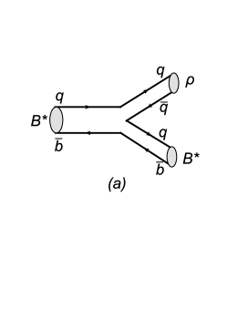
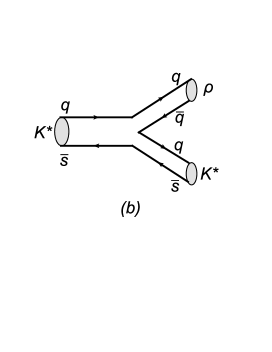
Figure 5: The vertex of $B^{*}B^{*}\rho$ and $K^{*}K^{*}\rho$ at the hadronic level.

In this subsection, we follow Refs. Liang:2014eba ; Soler:2015hna ; Sakai:2017avl and discuss the couplings in the Lagrangian. As an example, we consider the vertex of $B^{*}B^{*}\rho$. In order to estimate the corresponding coupling, we need to compare this vertex with that of $K^{*}K^{*}\rho$, since their topology is the same if the $\bar{s}$ and $\bar{b}$ quarks are seen as spectators. Fig. 5 shows the diagrams for these two vertices at the quark level, in which case the corresponding $S$ matrices should be the same, i.e.,

$$S^{mic} = 1-it\sqrt{\frac{2m_{L}}{2E_{L}}}\sqrt{\frac{2m^{\prime}_{L}}{2E^{\prime}_{L}}}\sqrt{\frac{1}{2\omega_{\rho}}}\frac{1}{\mathcal{V}^{3/2}}(2\pi)^{4}\delta(P_{in}-P_{out}).$$ (52)

On the other hand, at the hadronic level, the $S$ matrices are written as

$$S^{mac}_{B^{*}} = 1-it_{B^{*}}\frac{1}{\sqrt{2\omega_{B^{*}}}}\frac{1}{\sqrt{2\omega_{B^{*}}}}\frac{1}{\sqrt{2\omega_{\rho}}}\frac{1}{\mathcal{V}^{3/2}}(2\pi)^{4}\delta(P_{in}-P_{out}),$$ (53)

$$S^{mac}_{K^{*}} = 1-it_{K^{*}}\frac{1}{\sqrt{2\omega_{K^{*}}}}\frac{1}{\sqrt{2\omega_{K^{*}}}}\frac{1}{\sqrt{2\omega_{\rho}}}\frac{1}{\mathcal{V}^{3/2}}(2\pi)^{4}\delta(P_{in}-P_{out}).$$ (54)

As discussed above, we should have $S^{mac}_{B^{*}}=S^{mac}_{K^{*}}$ which tells us that the corresponding $T$ matrices obey the relation at the threshold as follows

$$\frac{t_{B^{*}}}{t_{K^{*}}}=\frac{m_{B^{*}}}{m_{K^{*}}}.$$ (55)

If we use the Lagrangian in Eq. (18) and calculate the $T$ matrices of the processes in Fig. 5, we find that Eq. (55) holds automatically, when the $\rho$ is the exchanged (virtual) vector meson, because the amplitude has the $\partial^{\mu}\cong\partial^{0}$ operator acting on the external vectors. The coupling of $B^{*}B^{*}\rho$ in Eq. (18) implements correctly the field correction factor of Eq. (55). Since in this case the $b$ quark acts as a spectator in the vertex, automatically this amplitude is consistent with heavy quark spin symmetry manohar . Similar discussions can be applied to the $BB\rho$ vertex with respect to $KK\rho$, and we have

$$\frac{t_{B}}{t_{K}}=\frac{m_{B}}{m_{K}},$$ (56)

but this is what we obtain from Eq. (21) using SU(4) flavor symmetry. Effectively one is using SU(3) when the heavy quark is considered as a spectator. In summary, we apply the Lagrangians of section II-A, and this takes automatically into account all the elements discussed above.

III.2 The $\bar{K}^{*}B^{*}$ system

With the potentials given in above section, we solve the Bethe-Salpeter equation considering $\bar{K}^{*}B^{*}$, $\omega B_{s}^{*}$ and $\phi B_{s}^{*}$ coupled channels. And we obtain three bound states with $J=0,1,2$, using the cutoff $q_{max}$ around $1055\sim 1085$ MeV. The obtained mass is $5847.8\sim 5831.7$ MeV for the spin 2 state which is consistent with that of $B_{s2}^{*}(5840)$. With this $q_{max}$, we predict that the bound state with $J=0$ has a mass $5908.5\sim 5894.4$ MeV, and the one with $J=1$ has a mass of $5912.1\sim 5898.2$ MeV. In Fig. 6, we plot the line shape of the mass distribution of these three states. In the PDG Patrignani:2016xqp , the mass of $B_{s1}(5830)$ with spin 1 is smaller than that of $B_{s2}^{*}(5840)$. However, the generated bound state with spin 1 has a mass about $65$ MeV larger than that of the bound state with spin 2. Henceforth, it is difficult to explain the $B_{s1}(5830)$ as the $\bar{K}^{*}B^{*}$ bound state. In the next subsection, we will come back to this problem.

The T-matrix close to a pole behaves like

$$T_{ij} \approx \frac{g_{i}g_{j}}{z-z_{R}},$$ (57)

where $i,j=\bar{K}^{*}B^{*},\omega B_{s}^{*},\phi B_{s}^{*}$, $g_{i}$ is the coupling to the channel $i$, $Re(z_{R})$ gives the mass of the bound state, $Im(z_{R})$ the half width, and $z$ is the complex value of the Mandelstam variable $s$. The coupling for a certain channel is obtained as

$$g_{i}^{2} = \lim_{z\to z_{R}}T_{ii}(z-z_{R}).$$ (58)

The sign of the coupling to the $B^{*}\bar{K}^{*}$ channel is chosen as positive, and those for the other channels are then determined by the following formula

$$\frac{g_{i}}{g_{j}} = \lim_{z\to z_{R}}\frac{T_{ii}}{T_{ij}}.$$ (59)

Table 1: The couplings for $\bar{K}^{*}B^{*}$ systems mixing with $\omega B_{s}^{*},\phi B_{s}^{*}$ channels. Here we chose the typical value of the cut off as $1070$ MeV. All the values are given in units of MeV.

channel	J=0	J=1	J=2
$\bar{K}^{*}B^{*}$	45955	45070	49633
$\omega B_{s}^{*}$	-10696	-14810	-15017
$\phi B_{s}^{*}$	18614	15702	19409

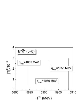
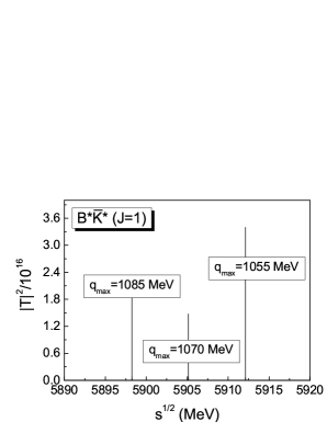
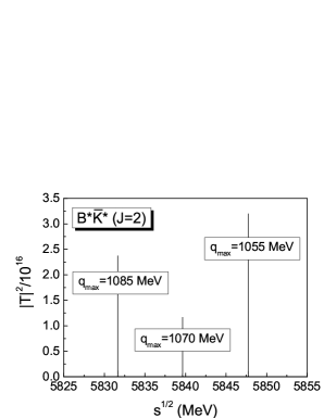
Figure 6: Squared amplitude for $\bar{K}^{*}B^{*}/\omega B_{s}^{*}/\phi B_{s}^{*}$ systems with spin 0, 1 and 2, respectively.

The value of the couplings are listed in Tab. 1, from which we can see that the $\bar{K}^{*}B^{*}$ component is dominant for all the states.

III.3 The $\bar{K}^{*}B$ system

As mentioned in the previous subsection, the $B_{s1}(5830)$ can not be explained as $\bar{K}^{*}B^{*}$ bound state with spin 1, since in PDG the mass of $B_{s1}(5830)$ is smaller than that of $B_{s2}^{*}(5840)$, which is contrary to our results. Now what we do is trying to explain the $B_{s1}(5830)$ under the $\bar{K}^{*}B/\omega B_{s}$ system.

Under hidden local symmetry there are no contact terms for $VVPP$ vertex, so that only vector exchange diagrams are involved. For the vector exchange terms, the interactions we study in this subsection have the same form as that of the $\bar{K}^{*}B/\omega B_{s}/\phi B_{s}$ interactions. So here we expect to find a bound state like in the case of the $\bar{K}^{*}B^{*}$ system. We use $q_{max}=1055\sim 1085$ MeV fixed in the case of $\bar{K}^{*}B^{*}$ bound state with spin 2. Then we obtain a pole position in the range of $5822.3\sim 5806.9$ MeV, which is consistent with the mass of $B_{s1}(5830)$ in the PDG. In Fig. 7, we plot the line shape of the $|T|^{2}$ depending on the center-of-mass energy $\sqrt{s}$. We also calculate the couplings, which have the value of $g_{\bar{K}^{*}B}=47654$, $g_{\omega B_{s}}=-13388$, $g_{\phi B_{s}}=18855$ with the cut off $q_{max}=1070$ MeV.

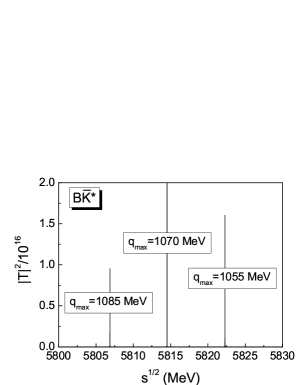
Figure 7: Squared amplitude for $\bar{K}^{*}B/\omega B_{s}/\phi B_{s}$ sector depending on the center-of-mass energy.

III.4 Other predictions

In this subsection, we will show the results corresponding to $\bar{K}B^{*}/\eta B_{s}^{*}$ and $\bar{K}B/\eta B_{s}$ interactions.

Like the case of $\bar{K}^{*}B/\omega B_{s}/\phi B_{s}$ system, there are no contact terms for $\bar{K}B^{*}/\eta B_{s}^{*}$ interaction. Only the vector meson exchange diagrams are considered. In Fig. 8, we plot the squared amplitude depending on the center-of-mass energy $\sqrt{s}$. Here, we also use the cut off $q_{max}=1055\sim 1085$ MeV as before. The pole position is located at $5671.2\sim 5663.6$ MeV. The couplings of $B^{*}\bar{K}$ and $B_{s}^{*}\eta$ are $30637$ MeV and $-13919$ MeV respectively, where we choose the cut off as 1070 MeV.

For $\bar{K}B/\eta B_{s}$ system, we predict a bound state with a mass of $5475.4\sim 5457.5$ MeV, and the couplings $g_{\bar{K}B}=53577$ MeV and $g_{\eta B_{s}}=-3689$ MeV, with a cut off $q_{max}=1070$ MeV.

In TABLE. 2, we list our results of all the systems.

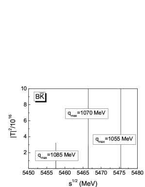
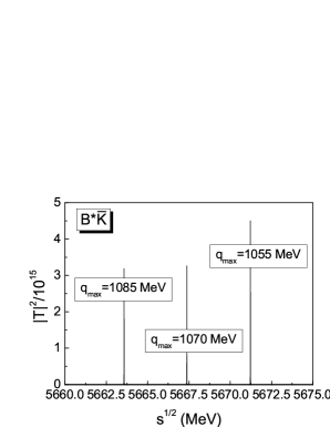
Figure 8: Squared amplitude for $\bar{K}B/\eta B_{s}$ and $\bar{K}B^{*}/\eta B_{s}^{*}$ sector.

Table 2: Summary of our results where the cut off is in the range of $1055\sim 1085$ MeV and the masses in this table is in the unit of MeV.

State mass	$I(J^{p})$	Main component	Exp.	State mass	$I(J^{p})$	Main component	Exp.
$5475.4\sim 5457.5$	$0(0^{+})$	$\bar{K}B$	-	$5908.5\sim 5894.4$	$0(0^{+})$	$\bar{K}^{*}B^{*}$	-
$5671.2\sim 5663.6$	$0(1^{+})$	$\bar{K}B^{*}$	-	$5912.1\sim 5898.2$	$0(1^{+})$	$\bar{K}^{*}B^{*}$	-
$5822.3\sim 5806.9$	$0(1^{+})$	$\bar{K}^{*}B$	$B_{s1}(5830)$	$5847.8\sim 5831.7$	$0(2^{+})$	$\bar{K}^{*}B^{*}$	$B_{s2}^{*}(5840)$

IV summary

In this work, we have studied the systems containing bottomed and strange quarks by the chiral unitary approach. Considering $\bar{K}^{*}B^{*}$ and $\omega B_{s}^{*}$ coupled channels and solving the Bethe-Salpeter equation, we find three states with masses $5908.5\sim 5894.4$ MeV, $5912.1\sim 5898.2$ MeV and $5847.8\sim 5831.7$ MeV, with the cut off $q_{max}$ chosen as $1055\sim 1085$ MeV. The state with spin 2 can be identified with $B_{s2}^{*}(5840)$. From the couplings that we obtained, we can see that the $\bar{K}^{*}B^{*}$ component is dominant. However, the $B_{s1}(5830)$ can not be explained as the state with spin 1, since its mass is smaller than that of $B_{s2}^{*}(5840)$. So we studied another system, i.e., $\bar{K}^{*}B/\omega B_{s}$ system, and we get a bound state with a mass $5822.3\sim 5806.9$ MeV which agrees with the mass of $B_{s1}(5830)$. In addition, we also studied $\bar{K}B^{*}/\eta B_{s}^{*}$ and $\bar{K}B/\eta B_{s}$ interactions, and predict two bound states with masses $5671.2\sim 5663.6$ MeV and $5475.4\sim 5457.5$ MeV, respectively. We expect further experiments to confirm our predictions.

References

- (1) M. Bando, T. Kugo, S. Uehara, K. Yamawaki and T. Yanagida, Phys. Rev. Lett. 54, 1215 (1985).
- (2) M. Bando, T. Kugo and K. Yamawaki, Phys. Rept. 164, 217 (1988).
- (3) U. G. Meissner, Phys. Rept. 161, 213 (1988).
- (4) M. Harada and K. Yamawaki, Phys. Rept. 381, 1 (2003)
- (5) R. Molina, D. Nicmorus and E. Oset, Phys. Rev. D 78, 114018 (2008)
- (6) L. S. Geng and E. Oset, Phys. Rev. D 79, 074009 (2009)
- (7) J. J. Xie, M. Albaladejo and E. Oset, Phys. Lett. B 728, 319 (2014)
- (8) X. L. Ren, L. S. Geng, E. Oset and J. Meng, Eur. Phys. J. A 50, 133 (2014)
- (9) R. Molina, H. Nagahiro, A. Hosaka and E. Oset, Phys. Rev. D 80, 014025 (2009)
- (10) P. del Amo Sanchez et al. [BaBar Collaboration], Phys. Rev. D 82, 111101 (2010)
- (11) R. Aaij et al. [LHCb Collaboration], JHEP 1309, 145 (2013)
- (12) R. Aaij et al. [LHCb Collaboration], Phys. Rev. D 94, no. 7, 072001 (2016)
- (13) P. Fernandez-Soler, Z. F. Sun, J. Nieves and E. Oset, Eur. Phys. J. C 76, no. 2, 82 (2016)
- (14) R. Akers et al. [OPAL Collaboration], Z. Phys. C 66, 19 (1995).
- (15) M. Moch [DELPHI Collaboration], PoS HEP 2005, 232 (2006).
- (16) R. K. Mommsen, Nucl. Phys. Proc. Suppl. 170, 172 (2007)
- (17) T. Aaltonen et al. [CDF Collaboration], Phys. Rev. Lett. 100, 082001 (2008)
- (18) V. M. Abazov et al. [D0 Collaboration], Phys. Rev. Lett. 100, 082002 (2008)
- (19) R. Aaij et al. [LHCb Collaboration], Phys. Rev. Lett. 110, no. 15, 151803 (2013)
- (20) W. H. Liang, C. W. Xiao and E. Oset, Phys. Rev. D 89, no. 5, 054023 (2014)
- (21) S. Sakai, L. Roca and E. Oset, Phys. Rev. D 96, no. 5, 054023 (2017)
- (22) A. V. Manohar and M. B. Wise, Camb. Monogr. Part. Phys. Nucl. Phys. Cosmol. 10, 1 (2000)
- (23) C. Patrignani et al. [Particle Data Group], Chin. Phys. C 40, no. 10, 100001 (2016). doi:10.1088/1674-1137/40/10/100001
- (24) E. Oset and A. Ramos, Eur. Phys. J. A 44, 445 (2010)
- (25) G. Ecker, J. Gasser, H. Leutwyler, A. Pich and E. de Rafael, Phys. Lett. B 223, 425 (1989).
- (26) H. Nagahiro, L. Roca, A. Hosaka and E. Oset, Phys. Rev. D 79, 014015 (2009)
- (27) W. H. Liang, J. M. Dias, V. R. Debastiani and E. Oset, arXiv:1711.10623 [hep-ph].
- (28) S. Okubo, Phys. Lett. 5, 165 (1963).
- (29) G. Zweig, Developments in the Quark Theory of Hadrons, Volume 1. Edited by D. Lichtenberg and S. Rosen. pp. 22-101
- (30) J. Iizuka, Prog. Theor. Phys. Suppl. 37, 21 (1966).
- (31) J. A. Oller, E. Oset and J. R. Pelaez, Phys. Rev. D 59, 074001 (1999) Erratum: [Phys. Rev. D 60, 099906 (1999)] Erratum: [Phys. Rev. D 75, 099903 (2007)]