Block-coordinate primal-dual method for the nonsmooth minimization over linear constraints

Abstract

We consider the problem of minimizing a convex, separable, nonsmooth function subject to linear constraints. The numerical method we propose is a block-coordinate extension of the Chambolle-Pock primal-dual algorithm. We prove convergence of the method without resorting to assumptions like smoothness or strong convexity of the objective, full-rank condition on the matrix, strong duality or even consistency of the linear system. Freedom from imposing the latter assumption permits convergence guarantees for misspecified or noisy systems.

2010 Mathematics Subject Classification: 49M29 65K10 65Y20 90C25

Keywords: Saddle-point problems, first order algorithms, primal-dual algorithms, coordinate methods, randomized methods

1 Introduction

We propose a randomized coordinate primal-dual algorithm for convex optimization problems of the form

$$\min_{x}g(x)\quad\text{s.t.}\quad x\in\operatorname{argmin}_{z}\frac{1}{2}\|Az-b\|^{2}.$$ (1)

This is a generalization of the more commonly encountered linear constrained convex optimization problem

$$\min_{x}g(x)\quad\text{s.t.}\quad Ax=b.$$ (2)

When $b$ is in the range of $A$ problem (2) and (1) have the same optimal solutions; but (1) has the advantage of having solutions even when $b$ is not in the range of $A$. Such problems will be called inconsistent in what follows. Of course, the solution set to (1) can be modeled by a problem with the format (2) via the normal equations. The main point of this note, however, is that the two models suggest very different algorithms with different behaviors, as explained in malitsky2017 and in Section 2 below.

We do not assume that $g$ is smooth, but this is not our main concern. Our main focus in this note is the efficient use of problem structure. In particular, we assume throughout that the problem can be decomposed in the following manner. For $x\in\mathbb{R}^{n}$, $A\in\mathbb{R}^{m\times n}$

$$A=[A_{1},\dots,A_{p}]\quad\mbox{ and }\quad g(x)=\sum_{i=1}^{p}g_{i}(x_{i}),$$

where $x_{i}\in\mathbb{R}^{n_{i}}$, $\sum_{i=1}^{p}n_{i}=n$, $A_{i}\in\mathbb{R}^{m\times n_{i}}$ and $g_{i}:\mathbb{R}^{n_{i}}\to(-\infty,+\infty]$ is proper, convex and lower semi-continuous (lsc). The coordinate primal-dual method we propose below allows one to achieve improved stepsize choice, tailored to the individual blocks of coordinates. To this, we add an intrinsic randomization to the algorithm which is particularly well suited for large-scale problems and distributed implementations. Another interesting property of the proposed method is that in the absence of the existence of Lagrange multipliers one can still obtain meaningful convergence results.

Randomization is currently the leading technique for handling extremely large-scale problems. Algorithms employing some sort of randomization have been around for more than 50 years, but they have only recently emerged as the preferred – indeed, sometimes the only feasible – numerical strategy for large-scale problems in machine learning and data analysis. The dominant randomization strategies can be divided roughly into two categories. To the first category belong stochastic methods, where in every iteration the full vector is updated, but only a fraction of the given data is used. The main motivation behind such methods is to generate descent directions cheaply. The prevalent methods SAGA defazio2014saga and SVR johnson2013accelerating belong to this group. Another category is coordinate-block methods. These methods update only one coordinate (or one block of coordinates) in every iteration. As with stochastic methods, the per iteration cost is very low since only a fraction of the data is used, but coordinate-block methods can also be accelerated by choosing larger step sizes. Popular methods that belong to this group are nesterov2012efficiency ; fercoq2015accelerated . A particular class of coordinate methods is alternating minimization methods, which appear to be a promising approach to solving nonconvex problems, see attouch2010proximal ; bolte2014proximal ; hesse2015proximal .

To keep the presentation simple, we eschew many possible generalizations and extensions of our proposed method. For concreteness we focus our attention on the primal-dual algorithm (PDA) of Chambolle-Pock chambolle2011first . The PDA is a well-known first-order method for solving saddle point problems with nonsmooth structure. It is based on the proximal mapping associated with a function $g$ defined by $\operatorname{prox}_{\tau g}=(\operatorname{Id}+\tau\partial g)^{-1}$ where $\partial g(\bar{x})$ is the convex subdifferential of $g$ at $\bar{x}$, defined as the set of all vectors $v$ with

$$g(x)-g(\bar{x})-\langle{v},{x-\bar{x}}\rangle\geq 0\quad\forall x.$$ (3)

The PDA applied to the Lagrangian of problem (2) generates two sequences $(x^{k}),(y^{k})$ via

$$x^{k+1} =\operatorname{prox}_{\tau g}(x^{k}-\tau A^{T}y^{k})$$ (4)

$$y^{k+1} =y^{k}+\sigma(A(2x^{k+1}-x^{k})-b).$$

Alternative approaches such as the alternating direction method of multipliers Glowinski75 are also currently popular for large-scale problems and are based on the augmented Lagrangian of (2). The advantage of PDA over ADMM, however, is that it does not require one to invert the matrix $A$, and hence can be applied to very large-scale problems. The PDA is very similar, in fact, to a special case of the proximal point algorithm he-yuan:2012 and of the so-called proximal ADMM shefi2014rate ; eckstein1994some ; banert2016fixing .

1:  Choose $x^{0}\in\mathbb{R}^{n}$, $\sigma>0$, $\tau\in\mathbb{R}^{p}_{++}$ and set $y^{0}=u^{0}=\sigma(Ax^{0}-b)$.

2:  for  $k=0,1,2,\dots$ do

3:     $x^{k+1}=x^{k}$

4:     Pick an index $i\in\{1,\dots,p\}$ uniformly at random.

5:     $x^{k+1}_{i}=\operatorname{prox}_{\frac{\tau_{i}}{p}g_{i}}(x^{k}_{i}-\frac{\tau_{i}}{p}A^{T}_{i}y^{k})$, $t_{i}=x^{k+1}_{i}-x^{k}_{i}$

6:     $y^{k+1}=y^{k}+u^{k}+\sigma(p+1)A_{i}t_{i}$

7:     $u^{k+1}=u^{k}+\sigma A_{i}t_{i}$

8:  end for

Algorithm 1 Coordinate primal-dual algorithm

The procedure we study in this note is given in Algorithm 1. The cost per iteration is very low: it requires two dot products $A_{i}t_{i}$, $A^{T}_{i}y^{k}$; and the full vector-vector operation is needed only for the dual variables $y^{k},u^{k}$ in steps $6$–$7$. The algorithm will therefore be the most efficient if $m\leq n$. If in particular all blocks are of size $1$, that is $n_{i}=1$, $n=p$ and $A_{i}$ is just the $i$-th column of the matrix $A$, then $A_{i}t_{i}$ reduces to the vector-scalar multiplication and $A_{i}^{T}y^{k}$ to the vector-vector dot product. Moreover, if the matrix $A$ is sparse and $A_{i}$ is its $i$-th column, then step $7$ requires an update of only those coordinates which are nonzero in $A_{i}$. The memory storage is also relatively small: we have to keep $x^{k}$, and two dual variables $y^{k}$, $u^{k}$. Another important feature of the proposed algorithm is that it is well suited for the distributed optimization: since there are no operations with a full primal vector, we can keep different blocks $x_{i}$ on different machines which are coupled only over dual variables.

We want to highlight that with $p=1$ the proposed algorithm indeed coincides with the primal-dual algorithm of Chambolle-Pock chambolle2011first . In fact, in this case it is not difficult to prove by induction that $u^{k}=\sigma(Ax^{k}-b)$ and hence, $y^{k+1}=y^{k}+\sigma(A(2x^{k+1}-x^{k})-b)$.

To the best of our knowledge the first randomized extension of Chambolle-Pock algorithm can be found in zhang2015stochastic . This method was proposed for solving the empirical risk minimization problem and is very popular for such kinds of problems. However, it converges under quite restrictive assumptions that never hold for problem (2), see more details in Section 2. Another interesting coordinate extension of the primal-dual algorithm is studied in fercoq2015coordinate . This does not require any special assumptions like smoothness or strong convexity, but, unfortunately, it requires an increase in the dimensionality of the problem, which for our targeted problems is counterproductive.

Recently there have also appeared coordinate methods for abstract fixed point algorithms combettes2015stochastic ; iutzeler2013asynchronous . Although they provide a useful and general way for developing coordinate algorithms, they do not allow the use of larger stepsizes — one of the major advantages of coordinate methods.

There are also some randomized methods for a particular choice of $g$ in (2). For $g\equiv 0$ paper strohmer2009randomized proposes a stochastic version of the Kaczmarz method, see also leventhal2010randomized and a nice review wright2015coordinate . When $g$ is the elastic net regularization (sum of $l_{1}$ and squared $l_{2}$ norms), papers lorenz2014linearized ; schopfer2016linear provide a stochastic sparse Kaczmarz method. Those methods belong to the first category of randomized methods by our classification, i.e., in every iteration they require an update of the whole vector.

In malitsky2017 the connection between the primal-dual algorithm (4) and the Tseng proximal gradient method tseng08 was shown. On the other hand, paper fercoq2015accelerated provides a coordinate extension of the latter method for a composite minimization problem. Based on these two results we propose a coordinate primal-dual method which is an extension of the original PDA. The key feature of Algorithm 1 is that it requires neither strong duality nor the consistency of the system $Ax=b$ to achieve good numerical performance with convergence guarantees. This allows us, for instance, to recover the signals from noisy measurements without any knowledge about the noise or without the need to tune some external parameters as one must for lasso or basis denoising problems chen2001atomic ; candes2006stable .

In the next section we provide possible applications and connections to other approaches in the literature. Section 3 is dedicated to the convergence analysis of our method. We also give an alternative form of the method and briefly discuss possible generalizations of the method. Finally, Section 4 details several numerical examples.

2 Applications

We briefly mention a few of the more prominent applications for Algorithm 1. We begin with the simplest of these.

Linear programming. The linear programming problem

$$\min_{x}\,\langle c,~{}x\rangle\quad\text{s.t. }\,Ax=b,\quad x\geq 0$$ (5)

is a special case of (2) with $g(x)=\langle c,~{}x\rangle+\delta_{x\geq 0}(x)$. In this case $g$ is fully separable. As a practical example, one can consider the optimal transport problem (see for instance santambrogio2015optimal ).

Composite minimization. The composite minimization problem

$$\min_{v}f(Kv)+r(v),$$ (6)

where both $f,r$ are convex functions, $v\in\mathbb{R}^{q}$, and $K\in\mathbb{R}^{m\times q}$ is a linear operator. For simplicity assume that both $f$ and $r$ are nonsmooth but allow for easy evaluation of the associated proximal mappings. In this case the PDA in chambolle2011first is a widely used method to solve such problems. It is applied to (6) written in the primal-dual form

$$\min_{v}\max_{w}r(v)+\langle Kv,w\rangle-f^{*}(w).$$ (7)

Alternatively, one can recast (6) in the form (2). To see this, let $x=(v,w)$, $g(x)=r(v)+f(w)$, and $Ax=Kv-w$. Then (6) is equivalent to

$$\min_{x}g(x)\quad\text{s.t.}\quad Ax=0.$$ (8)

Such reformulation is typical for the augmented Lagrangian method or ADMM boyd2011distributed . However, this is not very common to do for the primal-dual method, since problem (7) is already simpler than (8). Although the number of matrix-vector operations for both applications of the PDA remains the same, in (8) we have a larger problem: $x\in\mathbb{R}^{m+q}$, and the multiplier $y\in\mathbb{R}^{m}$ instead of $v\in\mathbb{R}^{q}$, $w\in\mathbb{R}^{m}$. However, the advantage for formulation (8) over (7) is that the updates of the most expensive variable $x=(v,w)$ can be done in parallel, in contrast to the sequential update of $v$ and $w$ when we apply PDA to (7).

Still, the main objection to (8) is that PDA treats the matrix $A$ as a black box – it does not exploit its structure. In particular, we have $\lambda(A)=\lambda(K)+1$ which globally defines the stepsizes. But in our case $A=[\begin{array}[]{c|c}K&-I\end{array}]$, whose structure is very tempting to use: for the block $w$ in $x=(v,w)$ we would like to apply larger steps that come from $\lambda(I)=1\leq\lambda(K)$ (the last inequality is typical). Fortunately, the proposed algorithm does exactly this: for each block the steps are defined only by the respective block of $A$. This is very similar in spirit to the proximal heterogeneous implicit-explicit method studied in hesse2015proximal . Notice that the paper pock2011diagonal provides only the possibility to use different weights for different blocks but it does not allow one to enlarge stepsizes. In  malitsky2016first a linesearch strategy is introduced that in fact allows one to use larger steps, but still this enlargement is based on the inequalities for the whole matrix $A$ and the vector $x$. Fercoq and Bianchi fercoq2015coordinate propose an extension (coordinate) of the primal-dual method that takes into account the structure of the linear operator, but this modification requires to increase the dimension of the problem.

Algorithm 1 can be applied without any smoothing of the nonsmooth functions $f$ and $r$. This is different from the approach of zhang2015stochastic ; palaniappan2016stochastic , where the convergence is only shown when the fidelity term $f$ is smooth and the regularizer $r$ is strongly convex.

Distributed optimization. The aim of distributed optimization over a network is to minimize a global objective using only local computation and communication. Problems in contemporary statistics and machine learning might be so large that even storing the input data is impossible in one machine. For applications and more in-depth overview we refer the reader to boyd2011distributed ; duchi2012dual ; Bertsekas:1989 ; nedic2010constrained and the references therein.

By construction, Algorithm 1 is distributed and hence ideally suited for these types of problems. Indeed, we can assign to the $i$-th node of our network the block of variables $x^{i}$ and the respective block matrix $A_{i}$. The dual variables $y$ and $u$ reside on the central processor. In each iteration of the algorithm implemented with this architecture only one random node is activated, requiring communication of the current dual vector $y^{k}$ from the central processor in order to compute the update to the block $x_{i}$. The node then returns $A_{i}t_{i}$ to the central processor.

The model problem (2) is also particularly well-suited for a distributed optimization. Suppose we want to minimize a convex function $f\colon\mathbb{R}^{m}\to(-\infty,+\infty]$. A common approach is to assign for each node a copy of $x$ and solve a constrained problem (the product space formulation):

$$\min_{x_{1},\dots,x_{p}}f(x_{1})+\dots+f(x_{p})\quad\text{s.t.}\quad x_{1}=\dots=x_{p}.$$ (9)

In fact, instead of $x_{1}=\dots=x_{p}$ we can introduce a more general but equivalent constraint $Ax=0$, where $x=(x_{1},\dots,x_{p})$ and the matrix $A$ describes the given network. By this, we arrive at the following problem

$$\min_{x}g(x)\quad\text{s.t.}\quad Ax=0,$$ (10)

where $g(x)=f(x_{1})+\dots+f(x_{p})$ is a separable convex function. Solving such problems in a stochastically, where in every iteration only one or few nodes are activated, has attracted a lot of attention recently, see latafat2017new ; fercoq2015coordinate ; bianchi2014stochastic .

Inverse problems. Linear systems remain a central occupation of inverse problems. The interesting problems are ill-posed and the observed data $A$, $b$ is noisy, requiring an appropriate regularization. A standard way is to consider either

$$\min_{x}g(x)+\frac{\delta}{2}\|Ax-b\|^{2}\qquad\text{or}\qquad\min_{x}g(x)\quad\text{s.t.}\quad\|Ax-b\|\leq\delta,$$ (11)

where $g$ is the regularizer which describes our a priori knowledge about a solution and $\delta>0$ is some parameter. The issue of how to choose this parameter is a major concern of numerical inverse problems. For the right hand-side problem this is easier to do: usually $\delta$ corresponds to the noise level of the given problem, but the optimization problem itself is harder than the left one due to the nonlinear constraints. Nevertheless, it can be still efficiently solved via PDA. Let $y=Ax-b$ and $h$ be the indicator function of the closed ball $B(0,\delta)$. Then the above problem can be expressed as

$$\min_{x,y}g(x)+h(y)\quad\text{s.t.}\quad Ax-y=b,$$ (12)

which is a particular case of (2). Again the coordinate primal-dual method, in contrast to the original PDA, has the advantage of exploiting the structure of the matrix $[\begin{array}[]{c|c}A&-I\end{array}]$ which allows one to use larger steps for faster convergence of the method.

There is another approach which we want to discuss. In many applications we do not need to solve a regularized problem exactly, the so-called early stopping may even help to obtain a better solution. Theoretically, one can consider another regularized problem: $\min_{x}g(x)$ such that $Ax=b$. Since during iteration we can easily control the feasibility gap $\|Ax^{k}-b\|$, we do not need to converge to a feasible solution $x^{*}$, where $Ax^{*}=b$, but stop somewhere earlier. The only issue with such approach is that the system $Ax=b$ might be inconsistent (and due to the noise this is often the case). Hence to be precise, we have to solve the following problem

$$\min_{x}g(x)\quad\text{s.t.}\quad x\in\operatorname{argmin}_{z}\bigl{\{}f(z):=\frac{1}{2}\|Az-b\|^{2}\bigr{\}}.$$ (13)

Obviously, the above constraint is equivalent to the $A^{T}Ax=A^{T}b$. Fortunately, we are able to show that our proposed method (without any modification) in fact solves (13), so it does not need to work with $A^{T}A$ that standard analysis of PDA requires. Notice that $A^{T}A$ is likely to be less sparse and more ill-conditioned than $A$.

3 Analysis

We first introduce some notation. For any vector $\omega=(\omega_{1},\dots,\omega_{p})\in\mathbb{R}^{p}_{++}$ we define the weighted norm by $\|x\|_{\omega}^{2}:=\sum\omega_{i}\|x_{i}\|^{2}$ and the weighted proximal operator $\operatorname{prox}_{g}^{\omega}$ by

$$\operatorname{prox}_{g}^{\omega}:=(\operatorname{Id}+\operatorname{Diag}(\omega^{-1})\circ\partial g)^{-1}=(\operatorname{Diag}(\omega)+\partial g)^{-1}\circ\operatorname{Diag}(\omega).$$

The weighted proximal operator has the following characteristic property (prox-inequality):

$$\bar{x}=\operatorname{prox}_{g}^{\omega}z\quad\Leftrightarrow\quad\langle\operatorname{Diag}(\omega)(\bar{x}-z),~{}x-\bar{x}\rangle\geq g(\bar{x})-g(x)\quad\forall x\in\mathbb{R}^{n}.$$ (14)

From this point onwards we will fix

$$f(x):=\frac{1}{2}\|Ax-b\|^{2}.$$ (15)

Then $\nabla f(x)=A^{T}(Ax-b)$ and its partial derivative corresponding to $i$-th block is $\nabla_{i}f(x)=A_{i}^{T}(Ax-b)$. Let $\lambda=(\lambda_{1},\dots,\lambda_{p})$, where $\lambda_{i}$ is the largest eigenvalue of $A_{i}^{T}A_{i}$, that is $\lambda_{i}=\lambda_{\max}(A_{i}^{T}A_{i})$. Then the Lipschitz constant of the $i$-th partial gradient is $\|A_{i}\|^{2}=\lambda_{i}$. By $U_{i}\colon\mathbb{R}^{n}\to\mathbb{R}^{n}$ we denote the projection operator: $U_{i}x=(0,\dots,x_{i},\dots,0)$. Since $f$ is quadratic, it follows that for any $x,y\in\mathbb{R}^{n}$

$$f(y)-f(x)-\langle\nabla f(x),y-x\rangle=\frac{1}{2}\|A(x-y)\|^{2}.$$ (16)

We also have that for any $x,t\in\mathbb{R}^{n}$

$$f(x+U_{i}t)=f(x)+\langle\nabla f(x),~{}U_{i}t\rangle+\frac{1}{2}\|A_{i}t_{i}\|^{2}\leq f(x)+\langle\nabla f(x),~{}U_{i}t\rangle+\frac{\lambda_{i}}{2}\|t_{i}\|^{2}.$$ (17)

Now since $i$ is a uniformly distributed random number over $\{1,2,\dots,p\}$, from the above it follows

$$\mathbb{E}[f(x+U_{i}t)]\leq f(x)+\frac{1}{p}\langle\nabla f(x),~{}t\rangle+\frac{1}{2p}\|t\|^{2}_{\lambda}.$$ (18)

For our analysis it is more convenient to work with Algorithm 2 given below. It is equivalent to Algorithm 1 when the random variable $i$ for the blocks are the same, though this might be not obvious at first glance. We give a short proof of this fact. Notice also that Algorithm 2 is entirely primal. The formulation of Algorithm 2 with $p=1$ (not random!) is related to the Tseng proximal gradient method malitsky2017 ; tseng08 and to its stochastic extension, the APPROX method fercoq2015accelerated . The proposed method requires stepsizes: $\sigma>0$ and $\tau\in\mathbb{R}^{p}_{++}$. The necessary condition for convergence of Algorithms 1 and 2 is, as we will see, $\tau_{i}\sigma\|A_{i}\|^{2}<1$. We have strict inequality for the same reason that one needs $\tau\sigma\|A\|^{2}<1$ in the original PDA.

1:  Choose $x^{0}\in\mathbb{R}^{n}$, $\sigma>0$, $\tau\in\mathbb{R}^{p}_{++}$ and set $s^{0}=x^{0}$, $\theta_{0}=1$.

2:  for  $k=0,1,2,\dots$ do

3:     $z^{k}=\theta_{k}x^{k}+(1-\theta_{k})s^{k}$

4:     $x^{k+1}=x^{k}$, $s^{k+1}=z^{k}$

5:     Pick an index $i\in\{1,\dots,p\}$ uniformly at random.

6:     $x^{k+1}_{i}=\operatorname{prox}_{\frac{\tau_{i}}{p}g_{i}}(x^{k}_{i}-\frac{\tau_{i}\sigma}{p\theta_{k}}\nabla_{i}f(z^{k}))$

7:     $s^{k+1}_{i}=z^{k}_{i}+{p}{\theta_{k}}(x^{k+1}_{i}-x^{k}_{i})$

8:     $\theta_{k+1}=\frac{1}{k+2}$

9:  end for

Algorithm 2 Coordinate primal-dual algorithm (equivalent form)

Let $f_{*}=\min f$ and $S$ be the solution set of (1). Observe that if the linear system $Ax=b$ is consistent, then $f_{*}=0$ and $\operatorname{argmin}f=\{x\colon Ax=b\}$. Otherwise, $f_{*}>0$ and $\operatorname{argmin}f=\{x\colon A^{T}Ax=A^{T}b\}$. We will often use an important simple identity:

$$f(x)-f(\bar{x})=\frac{1}{2}\|A(x-\bar{x})\|^{2}\qquad(\forall x\in\mathbb{R}^{n})(\forall\bar{x}\in S).$$ (19)

Proposition 1

If the index $i$ selected at iteration $k$ in step $4$ of Algorithm 1 is identical to the index $i$ selected at iteration $k$ in step $5$ of Algorithm 2, then both algorithms with the same starting point $x^{0}$ generate the same sequence $(x^{k})$.

Proof

We show that from Algorithm 2 one can recover all iterates of Algorithm 1 by setting $y^{k}=\frac{\sigma}{\theta_{k}}(Az^{k}-b)$, $u^{k}=\sigma(Ax^{k}-b)$. Then the proposition follows, since with $\nabla_{i}f(x)=A_{i}^{T}(Ax-b)$ we have

$$x^{k+1}_{i}=\operatorname{prox}_{\frac{\tau_{i}}{p}g_{i}}(x^{k}_{i}-\frac{\tau_{i}\sigma}{p\theta_{k}}A^{T}_{i}(Az^{k}-b))=\operatorname{prox}_{\frac{\tau_{i}}{p}g_{i}}(x^{k}_{i}-\frac{\tau_{i}}{p}A^{T}_{i}y^{k}).$$

Evidently, for $k=0$, one has $y^{0}=\sigma(Az^{0}-b)=\sigma(Ax^{0}-b)=u^{0}$. Assume it holds for some $k\geq 0$. By step 3 in Algorithm 2, we have

$$Az^{k+1}=\theta_{k+1}Ax^{k+1}+(1-\theta_{k+1})As^{k+1}=\theta_{k+1}(Ax^{k}+A_{i}t_{i})+(1-\theta_{k+1})(Az^{k}+p\theta_{k}A_{i}t_{i}),$$

where we have used that $Ax^{k+1}=Ax^{k}+A_{i}t_{i}$. Hence,

$$\frac{\sigma}{\theta_{k+1}}(Az^{k+1}-b)=\sigma(Ax^{k}-b)+\frac{\sigma}{\theta_{k}}(Az^{k}-b)+\sigma(p+1)A_{i}t_{i}=u^{k}+y^{k}+\sigma(p+1)A_{i}t_{i},$$

thus $y^{k+1}=\frac{\sigma}{\theta_{k+1}}(Az^{k+1}-b)$. Finally, $\sigma(Ax^{k+1}-b)=u^{k}+\sigma A_{i}t_{i}=u^{k+1}$. ∎

We are now ready to state our main result. Since the iterates given by Algorithm 2 are random variables, our convergence result is of a probabilistic nature. Notice also that equalities and inequalities involving random variables should be always understood to hold almost surely, even if the latter is not explicitly stated.

Theorem 3.1

Let $(x^{k}),(s^{k})$ be given by Algorithm 2, $\tau_{i}\sigma\|A_{i}\|^{2}<1$ for all $i=1,\dots,p$, and $S$ be the solution set of (1). Then

1. If there exists a Lagrange multiplier for problem (1), then $(x^{k})$ and $(s^{k})$ converge a.s. to a solution of (1) and $f(x^{k})-f_{*}=o(1/k)$, $f(s^{k})-f_{*}=O(1/k^{2})$ a.s. for the feasibility residual (15).

2. If $S$ is a bounded set and $g$ is bounded from below, then almost surely all limit points of $(s^{k})$ belong to $S$ and $f(s^{k})-f_{*}=o(1/k)$.

The proof of Theorem 3.1 is based on several simple lemmas which we establish first. The next lemma uses the following notation for the full update, $\hat{x}^{k+1}$, of $x^{k}$ in the $k$-th iteration of Algorithm 2, namely

$$\hat{x}^{k+1}=\operatorname{prox}^{\tau^{-1}}_{g/p}\left(x^{k}-\frac{k+1}{p}\sigma\operatorname{Diag}(\tau)\nabla f(z^{k})\right).$$ (20)

Lemma 1

For any fixed $x\in\mathbb{R}^{n}$ and any $k\in\mathbb{N}$ the following inequality holds:

$$\frac{p}{2}\|\hat{x}^{k+1}-x^{k}\|^{2}_{\tau^{-1}}+\frac{\sigma}{\theta_{k}}\langle\nabla f(z^{k}),~{}\hat{x}^{k+1}-x\rangle+g(\hat{x}^{k+1})-g(x)\\ \leq\frac{p}{2}\|x^{k}-x\|^{2}_{\tau^{-1}}-\frac{p}{2}\|\hat{x}^{k+1}-x\|^{2}_{\tau^{-1}}.$$ (21)

Proof

By the prox-inequality (14) with $\hat{x}^{k+1}$ given by (20) we have

$$\langle\operatorname{Diag}(\tau^{-1})(\hat{x}^{k+1}-x^{k}),~{}x-\hat{x}^{k+1}\rangle+\frac{\sigma}{p\theta_{k}}\langle\nabla f(z^{k}),~{}x-\hat{x}^{k+1}\rangle\geq\frac{1}{p}(g(\hat{x}^{k+1})-g(x)).$$ (22)

The statement then follows from the identity

$$\langle\operatorname{Diag}(\tau^{-1})(\hat{x}^{k+1}-x^{k}),~{}x-\hat{x}^{k+1}\rangle=\frac{1}{2}\|x^{k}-x\|^{2}_{\tau^{-1}}-\frac{1}{2}\|\hat{x}^{k+1}-x\|^{2}_{\tau^{-1}}-\frac{1}{2}\|\hat{x}^{k+1}-x^{k}\|^{2}_{\tau^{-1}}.$$

∎

The next result provides a bound on the expectation of the residual at the $(k+1)$th iterate, conditioned on the $k$th iterate, which we denote by $\mathbb{E}_{k}$.

Lemma 2

For any $x^{*}\in S$

$$\frac{1}{\theta_{k}^{2}}\mathbb{E}_{k}[f(s^{k+1})-f_{*}]\leq\frac{1}{\theta_{k-1}^{2}}(f(s^{k})-f_{*})-(f(x^{k})-f_{*})+\frac{1}{\theta_{k}}\langle\nabla f(z^{k}),~{}\hat{x}^{k+1}-x^{*}\rangle\\ +\frac{p}{2}\|\hat{x}^{k+1}-x^{k}\|^{2}_{\lambda}.$$ (23)

Proof

First, by (18)

$$\mathbb{E}_{k}[f(s^{k+1})]\leq f(z^{k})+\theta_{k}\langle\nabla f(z^{k}),~{}\hat{x}^{k+1}-x^{k}\rangle+\theta_{k}^{2}\frac{p}{2}\|\hat{x}^{k+1}-x^{k}\|^{2}_{\lambda}.$$ (24)

Since $f$ is quadratic (15), by (16) we have

$$f(s^{k})-f(z^{k})=\langle\nabla f(z^{k}),s^{k}-z^{k}\rangle+\frac{1}{2}\|A(s^{k}-z^{k})\|^{2}\\ =\frac{\theta_{k}}{1-\theta_{k}}\langle\nabla f(z^{k}),z^{k}-x^{k}\rangle+\frac{1}{2}\|A(s^{k}-z^{k})\|^{2}.$$ (25)

By (16) and $\|\alpha a+(1-\alpha)b\|^{2}=\alpha\|a\|^{2}+(1-\alpha)\|b\|^{2}-\alpha(1-\alpha)\|a-b\|^{2}$, we have

$$f_{*}-f(z^{k})=f(x^{*})-f(z^{k})=\langle\nabla f(z^{k}),x^{*}-z^{k}\rangle+\frac{1}{2}\|A(z^{k}-x^{*})\|^{2}\\ =\langle\nabla f(z^{k}),x^{*}-z^{k}\rangle+\theta_{k}(f(x^{k})-f_{*})+(1-\theta_{k})(f(s^{k})-f_{*})-\frac{1}{2}\theta_{k}(1-\theta_{k})\|A(x^{k}-s^{k})\|^{2}.$$ (26)

Notice that $x^{k}-s^{k}=\frac{1}{\theta_{k}}(s^{k}-z^{k})$. Hence, summation of $\frac{1-\theta_{k}}{\theta_{k}}\eqref{bi2:3}$ and (26) yields

$$\frac{1-\theta_{k}}{\theta_{k}}f(s^{k})-\frac{1}{\theta_{k}}f(z^{k})+f_{*}=\langle\nabla f(z^{k}),x^{*}-x^{k}\rangle+\theta_{k}(f(x^{k})-f_{*})+(1-\theta_{k})(f(s^{k})-f_{*}),$$ (27)

from which we conclude

$$\frac{1}{\theta_{k}^{2}}f(z^{k})+\frac{1}{\theta}_{k}\langle\nabla f(z^{k}),x^{*}-x^{k}\rangle=\frac{(1-\theta_{k})^{2}}{\theta_{k}^{2}}f(s^{k})+\frac{2-\theta_{k}}{\theta_{k}}f_{*}-(f(x^{k})-f_{*}).$$ (28)

Now summing up (24) multiplied by $\frac{1}{\theta_{k}^{2}}$ and (28), and using the identity $\frac{1-\theta_{k}}{\theta_{k}}=\frac{1}{\theta_{k-1}}$, we obtain

$$\frac{1}{\theta_{k}^{2}}\mathbb{E}_{k}[f(s^{k+1})-f_{*}]\leq\frac{1}{\theta_{k-1}^{2}}(f(s^{k})-f_{*})-(f(x^{k})-f_{*})+\frac{1}{\theta_{k}}\langle\nabla f(z^{k}),\hat{x}^{k+1}-x^{*}\rangle\\ +\frac{p}{2}\|\hat{x}^{k+1}-x^{k}\|^{2}_{\lambda}.$$ (29)

∎

The conditional expectations have the following useful representations. Expanding the expectation

$$\mathbb{E}_{k}[\|x^{k+1}-x\|^{2}_{\tau^{-1}}]=\sum_{i=1}^{p}\tau_{i}^{-1}\mathbb{E}_{k}[\|x^{k+1}_{i}-x_{i}\|^{2}]\\ =\sum_{i=1}^{p}\tau_{i}^{-1}\bigl{(}\frac{1}{p}\|\hat{x}^{k+1}_{i}-x\|^{2}+\frac{p-1}{p}\|\hat{x}^{k}_{i}-x\|^{2}\bigr{)}=\frac{1}{p}\|\hat{x}^{k+1}-x\|^{2}_{\tau^{-1}}+\frac{p-1}{p}\|x^{k}-x\|^{2}_{\tau^{-1}}.$$

This yields

$$\mathbb{E}_{k}\Bigl{[}\frac{p^{2}}{2}\|x^{k+1}-x\|^{2}_{\tau^{-1}}\Bigr{]}=\frac{p}{2}\|\hat{x}^{k+1}-x\|^{2}_{\tau^{-1}}+\frac{p^{2}-p}{2}\|x^{k}-x\|^{2}_{\tau^{-1}}.$$ (30)

Another characterization we use follows similarly, namely

$$\mathbb{E}_{k}[g(x^{k+1})]=\sum_{i=1}^{p}\bigl{(}\frac{1}{p}g_{i}(\hat{x}_{i}^{k+1})+\frac{p-1}{p}g_{i}(x^{k}_{i})\bigr{)}=\frac{1}{p}g(\hat{x}^{k+1})+\frac{p-1}{p}g(x^{k})$$

which gives

$$\mathbb{E}_{k}[g(x^{k+1})]=\frac{1}{p}g(\hat{x}^{k+1})+\left(1-\frac{1}{p}\right)g(x^{k}).$$ (31)

The next technical lemma is the last of the necessary preparations before proceding to the proof of the main theorem.

Lemma 3

The identity $s^{k+1}=\sum_{j=0}^{k+1}\beta^{j}_{k+1}x^{j}$ holds where the coefficients $(\beta_{k+1}^{j})_{j=0}^{k+1}$ are nonnegative and sum to $1$. In particular,

$$\beta_{k+1}^{j}=\begin{cases}(1-\theta_{k})\beta^{j}_{k},&j=0,\dots,k-1,\\ p\theta_{k-1}(1-\theta_{k})-(p-1)\theta_{k},&j=k,\\ p\theta_{k},&j=k+1.\end{cases}$$ (32)

and $\beta_{k+1}^{k}+(p-1)\theta_{k}=(1-\theta_{k})\beta_{k}^{k}$.

Proof

It is easy to prove by induction. For the reference see Lemma 2 in fercoq2015accelerated . ∎

The proof of Theorem 3.1 consists of three parts. The first contains an important estimation, derived from previous lemmas. In the second and third parts we respectively and independently prove (i) and (ii). The condition in (ii) is not restrictive and often can be checked in advance without any effort. In contrast, verifying strong duality (existence of Lagrange multipliers) is usually very difficult.

Proof (Theorem 3.1)

Since $\tau_{i}\sigma\|A_{i}\|^{2}<1$ for all $i=1,\dots,p$, there exists $\varepsilon>0$ such that $\tau_{i}^{-1}-\sigma\|A_{i}\|^{2}\geq\varepsilon$. This yields for all $x\in\mathbb{R}^{n}$, $\|x\|_{\tau^{-1}}^{2}-\sigma\|x\|_{\lambda}^{2}\geq\|x\|_{\varepsilon}^{2}$.

By convexity of $g$,

$$g(s^{k})=g(\sum_{j=0}^{k}\beta_{k}^{j}x^{j})\leq\sum_{j=0}^{k}\beta_{k}^{j}g(x^{j})=:\hat{g}_{k}.$$

Let $\hat{F}_{k}:=\hat{g}_{k}+\sigma k(f(s^{k})-f_{*})\geq\hat{g}_{k}+\sigma k(f(s^{k})-f_{*})$.

By Lemma 3 and (31), it follows

$$\mathbb{E}_{k}[\hat{g}_{k+1}] =\mathbb{E}_{k}[\beta_{k+1}^{k+1}g(\hat{x}^{k+1})]+\sum_{j=0}^{k}\beta_{k+1}^{j}g(x^{j})$$ (33)

$$=\theta_{k}g(\hat{x}^{k+1})+((p-1)\theta_{k}+\beta_{k+1}^{k})g(x^{k})+\sum_{j=0}^{k-1}\beta_{k+1}^{j}g(x^{j})$$ (34)

$$=\theta_{k}g(\hat{x}^{k+1})+(1-\theta_{k})\beta_{k}^{k}g(x^{k})+(1-\theta_{k})\sum_{j=0}^{k-1}\beta_{k}^{j}g(x^{j})$$ (35)

$$=\theta_{k}g(\hat{x}^{k+1})+(1-\theta_{k})\sum_{j=0}^{k}\beta_{k}^{j}g(x^{j})=\theta_{k}g(\hat{x}^{k+1})+(1-\theta_{k})\hat{g}_{k}.$$ (36)

Let $x^{*}\in S$. Setting $x=x^{*}$ in (21) and adding to $\sigma$ times (23) yields

$$\frac{\sigma}{\theta_{k}^{2}}\mathbb{E}_{k}[f(s^{k+1})-f_{*}]\leq \frac{\sigma}{\theta_{k-1}^{2}}(f(s^{k})-f_{*})-\sigma(f(x^{k})-f_{*})+\frac{p}{2}\|x^{k}-x^{*}\|^{2}_{\tau^{-1}}$$ (37)

$$\!\!\!\!\!\!\!\!\!\!-\frac{p}{2}\|\hat{x}^{k+1}-x^{*}\|^{2}_{\tau^{-1}}-\frac{p}{2}\|\hat{x}^{k+1}-x^{k}\|^{2}_{\varepsilon}-(g(\hat{x}^{k+1})-g_{*}).$$ (38)

Summing up (30) with $x=x^{*}$, (36) multiplied by $1/\theta_{k}=(k+1)$, and (38), we obtain

$$\mathbb{E}_{k}\Bigl{[}\frac{p^{2}}{2}\|x^{k+1}-x^{*}\|^{2}_{\tau^{-1}}+(k+1)(\hat{F}_{k+1}-g_{*})\Bigr{]}\leq\frac{p^{2}}{2}\|x^{k}-x^{*}\|^{2}_{\tau^{-1}}+k(\hat{F}_{k}-g_{*})\\ -\sigma(f(x^{k})-f_{*})-\frac{p}{2}\|\hat{x}^{k+1}-x^{k}\|^{2}_{\varepsilon}.$$ (39)

If the term inside the expectation in (39), $V_{k}(x^{*}):=\frac{p^{2}}{2}\|x^{k}-x^{*}\|^{2}_{\tau^{-1}}+k(\hat{F}_{k}-g_{*})$, were nonnegative, then one could apply the supermartingale theorem Bertsekas:1989 to obtain almost sure convergence directly. In our case this term need not be nonnegative, however it suffices to have $V_{k}(x^{*})$ bounded from below. With the assumption that there exists a Lagrange multiplier $u^{*}$, we shall show this.

(i) Let $u^{*}$ be a Lagrange multiplier for a solution $x^{*}$ to problem (1). Then by definition of the saddle point we have

$$g(s^{k})-g_{*}=g(s^{k})-g(x^{*}) \geq \langle A^{T}Au^{*},s^{k}-x^{*}\rangle$$ (40)

$$\geq -\|Au^{*}\|\cdot\|A(s^{k}-x^{*})\|=-\delta\sqrt{f(s^{k})-f_{*}},$$

where we have used (19) and denoted $\delta:=\sqrt{2}\|Au^{*}\|$. Our goal is to show that $k(\hat{F}_{k}-g_{*})$ is bounded from below. Indeed

$$k(\hat{F}_{k}-g_{*}) \geq k(g(s^{k})-g_{*})+\sigma k^{2}(f(s^{k})-f_{*})$$ (41)

$$\geq \frac{\sigma k^{2}}{2}(f(s^{k})-f_{*})+\left(\frac{\sigma k^{2}}{2}(f(s^{k})-f_{*})-\delta k\sqrt{f(s^{k})-f_{*}}\right).$$

The real-valued function $t\mapsto\frac{\sigma k^{2}}{2}t^{2}-\delta kt$ attains its smallest value $-\frac{\delta^{2}}{2\sigma}$ at $t=\frac{\delta}{\sigma k}$. Hence, we can deduce in (41) that

$$k(\hat{F}_{k}-g_{*})\geq\frac{\sigma k^{2}}{2}(f(s^{k})-f_{*})-\frac{\delta^{2}}{2\sigma}\geq-\frac{\delta^{2}}{2\sigma}.$$ (42)

We can then apply the supermartingale theorem to the shifted random variable $V_{k}(x^{*})+\delta^{2}/(2\sigma)$ to conclude that

$$\sum_{k=0}^{\infty}\sigma(f(x^{k})-f_{*})+\frac{p}{2}\|\hat{x}^{k+1}-x^{k}\|^{2}_{\varepsilon}<\infty\quad a.s.$$

and the sequence $V_{k}(x^{*})$ converges almost surely to a random variable with distribution bounded below by $-\frac{\delta^{2}}{2\sigma}$. Thus $(f(x^{k})-f_{*})=o(1/k)$, $\lim_{k\to\infty}\|\hat{x}^{k+1}-x^{k}\|_{\varepsilon}^{2}=0$ and, by the definition of $V_{k}(x^{*})$, the sequence $(x^{k})$ is pointwise a.s. bounded thus $k(\hat{F}_{k}-g_{*})$ is bounded above and hence, by (42), $f(s^{k})-f_{*}=O(1/k^{2})$ a.s.

By the definition of $z^{k}$ in step 3 of Algorithm 2 with $\theta_{k}=\frac{1}{k+1}$, we conclude that $f(z^{k})-f_{*}=O(1/k^{2})$ a.s. This yields a useful estimate:

$$\langle\nabla f(z^{k}),\hat{x}^{k+1}-x^{*}\rangle=\langle A^{T}(Az^{k}-b),\hat{x}^{k+1}-x^{*}\rangle=\langle A^{T}A(z^{k}-x^{*}),\hat{x}^{k+1}-x^{*}\rangle\\ \leq\|A(z^{k}-x^{*})\|\|A(\hat{x}^{k+1}-x^{*})\|=\sqrt{(f(z^{k})-f_{*})(f(\hat{x}^{k+1})-f_{*})}.$$ (43)

Since $f(\hat{x}^{k+1})-f_{*}\to 0$ a.s., we have $\frac{\sigma}{\theta_{k}}\langle\nabla f(z^{k}),\hat{x}^{k+1}-x^{*}\rangle\to 0$.

Now consider the pointwise sequence of realizations of the random variables $x^{k}$ over $\omega\in\Omega$ for which the sequence is bounded. Since these realizations of sequences are bounded, they possess cluster points. Let $x^{\prime}$ be one such cluster point. This point is feasible since in the limit $f(x^{\prime})-f_{*}=0$. Writing down inequality (22) for the convergent subsequence with $x=x^{*}$ and taking the limit we obtain $g(x^{\prime})\leq g(x^{*})$. Thus the pointwise cluster points $x^{\prime}\in S$ a.s.

We show next that the cluster points are unique. Again, for the same pointwise realization over $\omega\in\Omega$ as above, suppose there is another cluster point $x^{\prime\prime}$. By the argument above, $x^{\prime\prime}\in S$. The point $x^{*}\in S$ was arbitrary and so we can replace this by $x^{\prime}$. To reduce clutter, denote $\alpha_{k}=k(\hat{F}_{k}-g_{*})$ and denote the subsequence of $(x^{k})$ converging to $x^{\prime}$ by $\left(x^{k_{i}}\right)$ for $i\in\mathbb{N}$ and the subsequence converging to $x^{\prime\prime}$ by $\left(x^{k_{j}}\right)$ for $j\in\mathbb{N}$. We thus have

$$\lim_{k\to\infty}V_{k}(x^{\prime}) =\lim_{i\to\infty}V_{k_{i}}(x^{\prime})=\lim_{i\to\infty}(\frac{p^{2}}{2}\|x^{k_{i}}-x^{\prime}\|^{2}_{\tau^{-1}}+\alpha_{k_{i}})=\lim_{i\to\infty}\alpha_{k_{i}}$$ (44)

$$=\lim_{j\to\infty}V_{k_{j}}(x^{\prime})=\lim_{j\to\infty}(\frac{p^{2}}{2}\|x^{k_{j}}-x^{\prime}\|^{2}_{\tau^{-1}}+\alpha_{k_{j}})=\|x^{\prime\prime}-\tilde{x}_{1}\|^{2}_{\tau^{-1}}+\lim_{j\to\infty}\alpha_{k_{j}},$$ (45)

from which $\lim_{i\to\infty}\alpha_{k_{i}}=\frac{p^{2}}{2}\|x^{\prime\prime}-x^{\prime}\|^{2}_{\tau^{-1}}+\lim_{j\to\infty}a_{k_{j}}$ follows. Similarly, replacing $\tilde{x}$ with $x^{\prime\prime}$, we derive $\lim_{j\to\infty}\alpha_{k_{j}}=\frac{p^{2}}{2}\|\tilde{x}_{1}-x^{\prime\prime}\|^{2}_{\tau^{-1}}+\lim_{i\to\infty}\alpha_{k_{i}},$ from which we conclude that $x^{\prime}=x^{\prime\prime}$. Therefore, the whole sequence $(x^{k})$ converges pointwise almost surely to a solution.

Convergence of $(s^{k})$. First, recall from Lemma 3 that $s^{k}$ is a convex combination of $x^{j}$ for $j=0,\dots,k$. Second, notice that for all $j$, $\beta_{k+1}^{j}\to 0$ as $k\to\infty$. Hence, by the Toeplitz theorem (Exercise 66 in polya ) we conclude that $(s^{k})$ converges pointwise almost surely to the same solution as $(x^{k})$. By this, (i) is proved.

(ii) Taking the total expectation $\mathbb{E}$ of both sides of (39), we obtain

$$\mathbb{E}\bigl{[}V_{k+1}(x^{*})+\frac{p}{2}\|\hat{x}^{k+1}-x^{k}\|^{2}_{\varepsilon}\bigr{]}\leq\mathbb{E}[V_{k}(x^{*})].$$

Iterating the above,

$$\mathbb{E}\Bigl{[}\frac{p^{2}}{2}\|x^{k}-x^{*}\|^{2}_{\tau^{-1}}+k(\hat{F}_{k}-g_{*})+\sum_{i=1}^{k}\frac{p}{2}\|\hat{x}^{i}-x^{i-1}\|^{2}_{\varepsilon}\Bigr{]}\leq\frac{p^{2}}{2}\|x^{0}-x^{*}\|^{2}_{\tau^{-1}}=:C.$$ (46)

Since $g(s^{k})\leq\hat{g}_{k}$, one has

$$\mathbb{E}\Bigl{[}\frac{p^{2}}{2}\|x^{k}-x^{*}\|^{2}_{\tau^{-1}}+\sigma k^{2}(f(s^{k})-f_{*})+\sum_{i=1}^{k}\frac{p}{2}\|\hat{x}^{i}-x^{i-1}\|^{2}_{\varepsilon}\Bigr{]}\leq C+\mathbb{E}[k(g_{*}-g(s^{k}))].$$ (47)

From the above equation it follows that

$$\mathbb{E}\Bigl{[}\frac{p^{2}}{2k}\|x^{k}-x^{*}\|^{2}_{\tau^{-1}}+\sigma k(f(s^{k})-f_{*})\Bigr{]}\leq\frac{C}{k}+\mathbb{E}[g_{*}-g(s^{k})].$$ (48)

Recall that by our assumption, $g$ is bounded from below: let $g(x)\geq-l$ for some $l>0$. Thus, from (48) one can conclude that

$$\mathbb{E}[f(s^{k})-f_{*}]\leq\frac{C}{\sigma k^{2}}+\frac{g_{*}+l}{\sigma k}.$$

This means that almost surely $f(s^{k})-f_{*}=O(1/k)$. Later we will improve this estimation. Let $\Omega_{1}$ be an event of probability one such that for every $\omega\in\Omega_{1}$, $f(s^{k}(\omega))-f_{*}=O(1/k)$.

Boundedness of $(s^{k})$. First, we show that $(s^{i}(\omega))_{i\in\mathcal{I}}$ with $\mathcal{I}=\{i\colon g(s^{i})<g_{*}\}$ is a bounded sequence for every $\omega\in\Omega_{1}$. For this we revisit the arguments from solodov2007explicit ; malitsky2017 . By assumption the set $S=\{x\colon g(x)\leq g_{*},f(x)\leq f_{*}\}$ is nonempty and bounded. Consider the convex function $\varphi(x)=\max\{g(x)-g_{*},f(x)-f_{*}\}$. Notice that $S$ coincides with the level set $\mathcal{L}(0)$ of $\varphi$:

$$S=\mathcal{L}(0)=\{x\colon\varphi(x)\leq 0\}.$$

Since $\mathcal{L}(0)$ is bounded, the set $\mathcal{L}(c)=\{x\colon\varphi(x)\leq c\}$ is also bounded for any $c\in\mathbb{R}$. Fix any $c\geq 0$ such that $f(s^{k}(\omega))\leq c$ for all $k$ and $\omega\in\Omega_{1}$. Since $g(s^{i})-g_{*}<0\leq c$ for $i\in\mathcal{I}$, we have that for every $\omega\in\Omega_{1}$, $s^{i}(\omega)\in\mathcal{L}(c)$, which is a bounded set. Hence, $(s^{i}(\omega))_{i\in\mathcal{I}}$ is bounded for every $\omega\in\Omega_{1}$.

Note that from (47) we have a useful consequence: both sequences $(x^{j})$, $(\hat{x}^{j}-x^{j-1})$ with $j\notin\mathcal{I}$ are pointwise a.s. bounded. From this it follows immediately that for $j\notin\mathcal{I}$, $(x^{j}-x^{j-1})$ is pointwise a.s. bounded as well. Hence, there exists an event $\Omega_{2}$ of probability one such that $x^{j}(\omega)$, $(x^{j}-x^{j-1})(\omega)$ are bounded for each $\omega\in\Omega_{2}$. We now restrict ourselves to points $\omega\in\Omega_{1}\cap\Omega_{2}$. Clearly, the latter set has a probability one. Let $M_{\omega}$ be such a constant that, for $\omega\in\Omega_{1}\cap\Omega_{2}$

$$\|s^{i}(\omega)\|\leq M_{\omega}\quad \forall i\in\mathcal{I}$$ (49)

$$\|(x^{j}+(n-1)(x^{j}-x^{j-1}))(\omega)\|\leq M_{\omega}\quad \forall j\notin\mathcal{I}.$$

We prove by induction that the sequence $(s^{k}(\omega))$ is bounded, hence $(s^{k})$ is pointwise a.s.  bounded. Suppose that for index $k$, $\|s^{k}(\omega)\|\leq M_{\omega}$. If for index $k+1$, $g(s^{k+1}(\omega))<g_{*}$ then we are done: $k+1\in\mathcal{I}$ and hence, $\|s^{k+1}(\omega)\|\leq M_{\omega}$. If $g(s^{k+1}(\omega))\geq g_{*}$, then $(k+1)\notin\mathcal{I}$. By the definition of $s^{k}$ in Algorithm 2, $s^{k+1}=\theta_{k}(nx^{k+1}-(n-1)x^{k})+(1-\theta_{k})s^{k}$, and hence

$$\|s^{k+1}\|\leq\theta_{k}\|x^{k+1}+(n-1)(x^{k+1}-x^{k})\|+(1-\theta_{k})\|s^{k}\|,$$

which shows that $\|s^{k+1}(\omega)\|\leq M_{\omega}$. This completes the proof that $s^{k}(\omega)$ is bounded and hence $(s^{k})$ is pointwise a.s. bounded.

Convergence of $(s^{k})$. Recall that a.s. $f(s^{k})-f_{*}=O(1/k)$. Hence, all limit points of $s^{k}(\omega)$ are feasible for any $\omega\in\Omega_{1}\cap\Omega_{2}$. This means that for every $\omega\in\Omega_{1}\cap\Omega_{2}$, $\liminf_{k\to\infty}g(s^{k}(\omega))\geq g_{*}$. If one assumes that there exist an event $\Omega_{3}$ of non-zero probability such that for every $\omega\in\bigcap_{i=1}^{3}\Omega_{i}$, $\limsup_{k\to\infty}g(s^{k}(\omega))>g_{*}$, then taking the limit superior in (48), one obtains a contradiction. This yields that almost surely $\lim_{k\to\infty}g(s^{k})=g_{*}$ and hence, almost surely all limit points of $(s^{k})$ belong to $S$. Using the obtained result, we can improve the estimation for $f(s^{k})-f_{*}$. Now from (48) it follows that almost surely $f(s^{k})-f_{*}=o(1/k)$. ∎

3.1 Possible generalizations

Strong convexity. When $g$ is strongly convex in (2), the estimates in Theorem 3.1 can be improved and in case (ii) the convergence of $(s^{k})$ to the solution of (2) can be proved. For this one needs to combine the proposed analysis and the analysis from malitsky2017 .

Adding the smooth term and ESO. Instead, of solving (2), one can impose more structure for this problem:

$$\min_{x}g(x)+h(x)\quad\text{s.t.}\quad Ax=b,$$ (50)

where in addition to the assumptions in Section 1, we assume that $h\colon\mathbb{R}^{N}\to\mathbb{R}$ is a smooth convex function with a Lipschitz-continuous gradient $\nabla h$. In this case the new coordinate algorithm can be obtained by combining analysis from fercoq2015accelerated and malitsky2017 . The expected separable overapproximation (ESO), proposed in fercoq2015accelerated , can help here much more, due to the new additional term $h$.

Parallelization. For simplicity, our analysis has focused only on the update of one block in every iteration. Alternatively, one could choose a random subset of blocks and update all of them more or less by the same logic as in Algorithm 1. This is one of the most important aspects of the algorithm that provides for fast implementations. The analysis of such extension will involve only a bit more tedious expressions with expectation, for more details we refer again to fercoq2015accelerated , where this was done for the unconstrained case: $\min_{x}g(x)+h(x)$. More challenging is to develop an asynchronous parallel extension of the proposed method in the spirit of peng2016arock , but with the possibility of taking larger steps.

4 Numerical experiments

This section collects several numerical tests to illustrate the performance of the proposed methods. Computations were performed using Python 3.5 on a standard laptop running 64-bit Debian GNU/Linux.

4.1 Basis pursuit

For a given matrix $A\in\mathbb{R}^{m\times n}$ and observation vector $b\in\mathbb{R}^{m}$, we want to find a sparse vector $x^{\dagger}\in\mathbb{R}^{n}$ such that $Ax^{\dagger}=b$. In standard circumstances we have $m\ll n$, so the linear system is underdetermined. Basis pursuit, proposed by Chen and Donoho chen:basis_pursuit ; chen2001atomic , involves solving

$$\min_{x}\|x\|_{1}\quad\text{s.t.}\quad Ax=b.$$ (51)

In many cases it can be shown (see candes2008introduction and references therein) that basis pursuit is able to recover the true signal $x^{\dagger}$ even when $m\ll n$.

A simple observation says that problem (51) fits well in our framework. For given $m,n$ we generate the matrix $A\in\mathbb{R}^{m\times n}$ in two ways:

• Experiment 1: $A$ is a random Gaussian matrix, i.e. every entry of $A$ drawn from the normal distribution $\mathcal{N}(0,1)$. A sparse vector $x^{\dagger}\in\mathbb{R}^{n}$ is constructed by choosing at random $5\%$ of its entries independently and uniformly from $(-10,10)$.

• Experiment 2: $A=R\Phi$, where $\Phi\in\mathbb{R}^{n\times n}$ is the discrete cosine transform and $R\in\mathbb{R}^{m\times n}$ is the random projection matrix: $Rx$ randomly extracts $m$ coordinates from the given $x$. A sparse vector $x^{\dagger}\in\mathbb{R}^{n}$ is constructed by choosing at random $50$ of its entries among the first $100$ coordinates independently from the normal distribution $\mathcal{N}(0,1)$. The remaining entries of $x^{\dagger}$ are set to $0$.

For both experiments we generate $b=Ax^{\dagger}$. The starting point for all algorithms is $x^{0}=0$. For all methods we use the same stopping criteria:

$$\|Ax^{k}-b\|_{\infty}\leq 10^{-6}\quad\text{and}\quad\operatorname{dist}(-A^{T}y^{k},\partial_{\|\cdot\|_{1}}(x^{k}))_{\infty}\leq 10^{-6}.$$

For given $A$ and $b$ we compare the performance of PDA and the proposed methods: Block-PDA with $n_{\text{block}}=n/w$ blocks of the width $w$ each and Coo-PDA with every single coordinate as a block. In the first and the second experiments the width of blocks for the Block-PDA is $w=50$.

The numerical behavior of all three methods depends strongly on the choice of the stepsizes. It is easy to artificially handicap PDA in comparisons with almost any algorithm: just take very bad steps for PDA. To be fair, for every test problem we present the best results of PDA among all with steps $\sigma=\dfrac{1}{2^{j}\|A\|}$, $\tau=\dfrac{2^{j}}{\|A\|}$, for $j=-15,-14,\dots,15$. Instead, for the proposed methods we always take the same step $\sigma=\dfrac{1}{2^{j}n_{\text{block}}}$, where we set $j=11$ for the first experiment and $j=8$ for the second one.

Table 1: Comparison of PDA, Block-PDA and Coo-PDA for problem (51). Experiment 1

Algorithm		$m=1000$, $n=4000$			$m=2000$, $n=8000$			$m=4000$, $n=16000$
		epoch	CPU		epoch	CPU		epoch	CPU
PDA		777	24		815	89		829	333
Block-PDA		108	4		103	12		107	51
Coo-PDA		79	2		73	7		94	34

Tables 1 and 2 collect information of how many epochs and how much CPU time (in seconds) is needed for each method and every test problem to reach the $10^{-6}$ accuracy. The term “epoch” means one iteration of the PDA or $n_{\text{block}}$ iterations of the coordinate PDA. By this, after $k$ epochs the $i$-th coordinate of $x$ will be updated on average the same number of times for the PDA and our proposed method. The CPU time might be not a good indicator, since it depends on the platform and the implementation. However, the number of epochs gives an exact number of arithmetic operations. This is a fair benchmark characteristic.

Concerning the stepsizes, we reiterate that the PDA was always taken with the best steps for every particular problem: for the first experiment (when $A$ is Gaussian), the parameter $j$ was usually among $4,5,6,7$. For the second experiment, the best values of $j$ were among $0,\dots,6$.

Table 2: Comparison of PDA, Block-PDA and Coo-PDA for problem (51). Experiment 2

Algorithm		$m=1000$, $n=4000$			$m=2000$, $n=8000$			$m=4000$, $n=16000$
		epoch	CPU		epoch	CPU		epoch	CPU
PDA		303	9		284	29		286	122
Block-PDA		41	2		40	5		36	18
Coo-PDA		27	1		23	3		24	10

4.2 Basis pursuit with noise

In many cases, a more realistic scenario is when our measurements are noisy. Now we wish to recover a sparse vector $x^{\dagger}\in\mathbb{R}^{n}$ such that $Ax^{\dagger}+\varepsilon=b$, where $\varepsilon\in\mathbb{R}^{m}$ is the unknown noise. Two standard approaches chen2001atomic ; candes2006stable involve solving either the lasso problem or basis pursuit denoising:

$$\min_{x}\|x\|_{1}+\frac{\delta}{2}\|Ax-b\|^{2}\qquad\text{or}\qquad\min_{x}\|x\|_{1}\quad\text{s.t.}\quad\|Ax-b\|\leq\delta.$$ (52)

In order to recover $x^{\dagger}$, both problems require a delicate tuning of the parameter $\delta$. For this one usually requires some a priori knowledge about the noise.

Even with noise, we still apply our method to the plain basis pursuit problem

$$\min_{x}\|x\|_{1}\quad\text{s.t.}\quad Ax=b.$$ (53)

We know that the proposed method converges even when the linear system is inconsistent (and this is the case when $A$ is rank-deficient). First, we may hope that the actual solution $x^{*}$ of (53) to which the method converges is not far from the true $x^{\dagger}$. In fact, if the system $Ax=b$ is consistent, we have $\|A(x^{*}-x^{\dagger})\|=\varepsilon$. Similarly, if that system is inconsistent, by (19) we have $f(x^{\dagger})-f(x^{*})=\frac{1}{2}\|A(x^{\dagger}-x^{*})\|^{2}$. And hence, again we obtain $\|A(x^{\dagger}-x^{*})\|^{2}\leq 2f(x^{\dagger})=\varepsilon^{2}$. Second, it might happen that the trajectory of $(x^{k})$ at some point is even closer to $x^{\dagger}$; in this case the early stopping can help to recover $x^{\dagger}$. In fact, as our simulations show, the convergence of the coordinate PDA to the actual solution $x^{*}$ is very slow, though, it is unusually fast in the beginning.

For given $m=1000,n=4000$ we generate two scenarios:

• $A\in\mathbb{R}^{m\times n}$ is a random Gaussian matrix.

• $A=A_{L}A_{R}$, where $A_{L}\in\mathbb{R}^{m\times m/2}$ and $A_{R}\in\mathbb{R}^{m/2\times n}$ are two random Gaussian matrices.

The latter condition guarantees that the rank of $A$ is at most $m/2$. Hence, with a high probability the system $Ax=b$ will be inconsistent due to the noise.

We generate a sparse vector $x^{\dagger}\in\mathbb{R}^{n}$ choosing at random $50$ of its elements independently and uniformly from $(-10,10)$. Then we define $b\in\mathbb{R}^{m}$ in two ways: either $b=Ax^{\dagger}+\varepsilon$, where $\varepsilon\in\mathbb{R}^{m}$ is a random Gaussian vector or $b$ is obtained by rounding off every coordinate of $Ax^{\dagger}$ to the nearest integer.

For simplicity we run only the block PDA with blocks of width $50$, thus we have $n_{\text{block}}=n/50$. The parameter $\sigma$ is chosen as $\sigma=\frac{1}{2^{25}n_{\text{block}}}$. After every $k$-th epoch we compute the signal error $\frac{\|x^{k}-x^{\dagger}\|}{\|x^{\dagger}\|}$ and the feasibility gap $\|A^{T}(Ax^{k}-b)\|$. The results are presented in Fig. 1, 2.

As one can see from the plots, the convergence of $(x^{k})$ to the best approximation of $x^{\dagger}$ takes place just after few epochs (less than 100). This convergence is very fast for both the signal error and the feasibility gap. After that, both lines switch to the slow regime: the signal error slightly increases and stabilizes after that; the feasibility gap decreases relatively slowly. Although in practice we do not know $x^{\dagger}$, we still can use early stopping, since both lines change their behavior approximately at the same time and it is easy to control the feasibility gap.

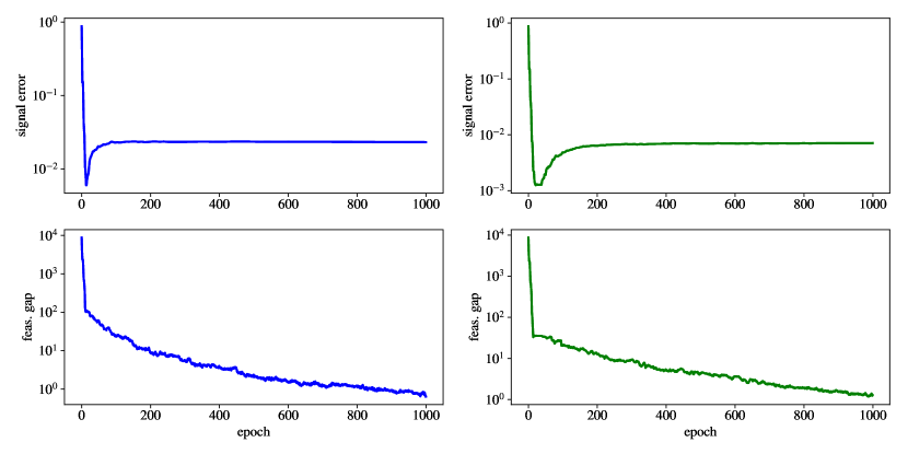
Figure 1: Convergence of block-PDA for noisy basis pursuit. $A$ is a random Gaussian matrix. Left (blue): problem with $b=Ax^{\dagger}+\varepsilon$, where $\varepsilon$ is a random Gaussian vector. Right (green): problem with $b$ obtained by rounding off $Ax^{\dagger}$ to the nearest integer. Top: signal error. Bottom: feasibility gap.

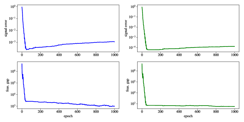
Figure 2: Convergence of block-PDA for noisy basis pursuit. $A$ is a low-rank matrix $A=A_{L}A_{R}$. Left (blue): problem with $b=Ax^{\dagger}+\varepsilon$, where $\varepsilon$ is a random Gaussian vector. Right (green): problem with $b$ obtained by rounding off $Ax^{\dagger}$ to the nearest integer. Top: signal error. Bottom: feasibility gap.

Finally, we would like to illustrate the proposed approach on a realistic non-sparse signal. We set $m=1000,n=4000$ and generate a random signal $w\in\mathbb{R}^{n}$ that has a sparse representation in the dictionary of the discrete cosine transform, that is $w=\Phi x^{\dagger}$ with the matrix $\Phi\in\mathbb{R}^{n\times n}$ is the discrete cosine transform and $x^{\dagger}\in\mathbb{R}^{n}$ is the sparse vector with only $50$ non-zero coordinates drawn from $\mathcal{N}(0,1)$. The measurements are modeled by a random Gaussian matrix $M\in\mathbb{R}^{m\times n}$. The observed data is corrupted by noise: $b=Mw+\varepsilon$, where $\varepsilon\in\mathbb{R}^{m}$ is a random vector, whose entries are drawn from $\mathcal{N}(0,10)$.

Obviously, we can rewrite the above equation as $b=Ax+\varepsilon$, where $A=M\Phi\in\mathbb{R}^{m\times n}$. We apply the proposed block-coordinate primal-dual method to the problem

$$\min_{x}\|x\|_{1}\quad\text{s.t.}\quad Ax=b$$ (54)

with $\sigma=\frac{1}{2^{22}n_{\text{block}}}$ and the width $50$ of each block. The behavior of the iterates $x^{k}$ is depicted in Figure 3. Figure 4 shows the true signal $w$ and the reconstructed signal $\hat{w}=\Phi x^{30}$ after $30$ epochs of the method. The signal error in this case is $\frac{\|\hat{w}-w\|}{\|w\|}=0.0036$. Interestingly, after $1000$ epochs we obtain the reconstructed signal $\hat{w}^{1000}$ for which the error is also quite reasonable: $\frac{\|\hat{w}^{1000}-w\|}{\|w\|}=0.016$.

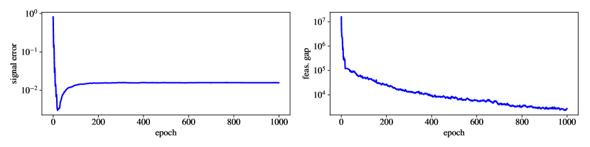
Figure 3: Convergence of block-PDA for noisy basis pursuit with a non-sparse signal. $A=M\Phi$. Left: signal error. Right: feasibility gap.

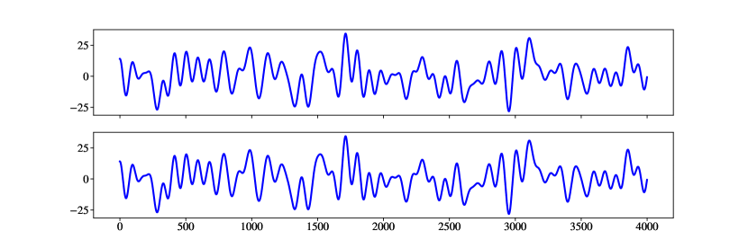
Figure 4: Top: original signal $w$. Bottom: reconstructed signal $\hat{w}$ after $30$ epochs. The signal error is $0.0036$.

Notice that we have reconstructed the signal without any knowledge about the noise. The only parameter which requires some tuning from our side was the stepsize $\sigma$. However, the method is not very sensitive to the choice of $\sigma$. In fact, we were able to reconstruct the signal at least for any $\sigma=\frac{1}{2^{j}n_{\text{block}}}$ for $j$ from the range $15,\dots,30$. Only the number of iterations of the method and the obtained accuracy changed, though still it was always enough for a good reconstruction.

4.3 Robust principal component analysis

Given the observed data matrix $M\in\mathbb{R}^{n_{1}\times n_{2}}$, robust principal component analysis aims to find a low rank matrix $L$ and a sparse matrix $S$ such that $M=L+S$. Problems which involve so many unknowns and the “low-rank” component should be difficult (in fact it is NP-hard), however, they can be successfully handled via robust principal component analysis, modeled by the following convex optimization problem

$$\min_{L,S}\|L\|_{*}+\lambda\|S\|_{1}\quad\text{s.t.}\quad L+S=M.$$ (55)

Here $\|L\|_{*}=\sum_{i}\sigma_{i}(L)$ is the nuclear norm of $L$, $\|S\|_{1}=\sum_{i,j}|S_{ij}|$, and $\lambda>0$. In candes2011robust ; wright2009robust it was shown that under some mild assumptions problem (55) indeed recovers the true matrices $L$ and $S$. The RPCA has many applications, see candes2011robust and the references therein.

Problem (55) is well-suited for both ADMM yuan2009sparse ; lin2010augmented and PDA. In fact, since the linear operator $A$ that defines the linear constraint has a simple structure $A=[\begin{array}[]{c|c}I&I\end{array}]$, those two methods almost coincide. Obviously, the bottleneck for both methods is computing the prox-operator with respect to the variable $L$, which involves computing a singular value decomposition (SVD). As (55) is a particular case of (2) with two blocks, one can apply the proposed coordinate PDA. In this case, in every iteration one should update either the $L$ block or the $S$ block. Hence, on average $k$ iterations of the method require only $k/2$ SVD. Keeping this in mind, we can hope for a faster convergence of our method compared to the original PDA.

For the experiment we use the settings from wright2009robust . For given $n_{1},n_{2}$ and rank $r$ we set $L^{\dagger}=Q_{1}Q_{2}$ with $Q_{1}\in\mathbb{R}^{n_{1}\times r}$ and $Q_{2}\in\mathbb{R}^{r\times n_{2}}$, whose elements are i.i.d. $\mathcal{N}(0,1)$ random variables. Then we generate $S^{\dagger}\in\mathbb{R}^{n_{1}\times n_{2}}$ as a sparse matrix whose $5\%$ non-zero elements are chosen uniformly at random from the range $[-500,500]$. We set $M=L^{\dagger}+S^{\dagger}$ and $\lambda=\frac{1}{\sqrt{n_{1}}}$.

The KKT optimality conditions for (55) yield

$$Y\in\partial(\lambda\|S\|_{1}),\qquad Y\in\partial(\|L\|_{*}),\qquad S+L-M=0,$$

which implies that $(L,S)$ is optimal whenever

$$\partial(\lambda\|S\|_{1})\cap\partial(\|L\|_{*})\neq\varnothing\quad\text{and}\quad S+L-M=0.$$

Since we do not want to compute $\partial(\|L\|_{*})$ and $\partial(\|S\|_{1})$, we just measure the distance between their two subgradients which we can compute from the iterates.

Given the current iterates $(L^{k},S^{k},Y^{k})$ for the PDA, we know that $\frac{1}{\tau}(L^{k-1}-L^{k})-Y^{k-1}\in\partial(\|L^{k}\|_{*})$ and $\frac{1}{\tau}(S^{k-1}-S^{k})-Y^{k-1}\in\partial(\|S^{k}\|_{1})$. Hence, we can terminate algorithm whenever

$$\frac{\|L^{k-1}-L^{k}+S^{k}-S^{k-1}\|}{\tau\|M\|}\leq\varepsilon\quad\text{and}\quad\frac{\|S^{k}+L^{k}-M\|_{\infty}}{\|M\|}\leq\varepsilon$$

where $\varepsilon>0$ is the desired accuracy. A similar criteria was used for the Coo-PDA termination.

We run several instances of PDA with stepsize $\tau=\frac{2^{j}}{L}$, $\sigma=\frac{1}{2^{j}L}$ for $j=-6,-5,\dots,12$, where $L=\sqrt{2}$ is the norm of the operator $A=[\begin{array}[]{c|c}I&I\end{array}]$. Similarly, we run several instances of Coo-PDA with $\tau=(1,1)$ and $\sigma=\frac{1}{2^{j}}$ for the same range of indices $j$. We show only the performance of the best instances for both methods, and it was always the case that $j\in\{6,7,8\}$. The accuracy $\varepsilon$ was set to $10^{-6}$. We also compare PDA-r and Coo-PDA-r, where instead of an exact SVD a fast randomized SVD solver was used. We chose the one from the scikit-learn library scikit-learn .

In Table 3 we show the benchmark for PDA and Coo-PDA with an exact evaluation of SVD and for PDA-r and Coo-PDA-r with randomized SVD. For different input data, the table collects the total number of iterations and the CPU time in seconds for all methods. Notice that for the Coo-PDA the number of evaluation of SVD is approximately half of the iterations, this is why it terminates faster.

We want to highlight that in all experiments the unknown matrix $L^{\dagger}$ was indeed recovered. And, as one can see from the Table 3, in all experiments the coordinate primal-dual algorithms performed better than the standard ones.

Table 3: Comparison of PDA and Coo-PDA for problem (55) with exact and approximate evaluation of SVD

$n_{1}$	$n_{2}$	$r$		PDA			Coo-PDA			PDA-r			Coo-PDA-r
				iter	CPU		iter	CPU		iter	CPU		iter	CPU
1000	500	20		161	173		219	121		104	39		159	29
1500	500	20		150	211		200	142		139	71		182	47
2000	500	50		154	279		205	185		130	87		180	61
1000	1000	50		188	1004		251	678		124	111		174	76
2000	1000	50		160	1355		200	879		91	146		120	95

- (1) H. Attouch, J. Bolte, P. Redont, and A. Soubeyran. Proximal alternating minimization and projection methods for nonconvex problems: An approach based on the Kurdyka-łojasiewicz inequality. Mathematics of Operations Research, 35(2):438–457, 2010.
- (2) S. Banert, R. I. Bot, and E. R. Csetnek. Fixing and extending some recent results on the admm algorithm. arXiv preprint arXiv:1612.05057, 2016.
- (3) D. P. Bertsekas and J. N. Tsitsiklis. Parallel and Distributed Computation: Numerical Methods. Prentice-Hall, Inc., Upper Saddle River, NJ, USA, 1989.
- (4) P. Bianchi, W. Hachem, and I. Franck. A stochastic coordinate descent primal-dual algorithm and applications. In Machine Learning for Signal Processing (MLSP), 2014 IEEE International Workshop on, pages 1–6. IEEE, 2014.
- (5) J. Bolte, S. Sabach, and M. Teboulle. Proximal alternating linearized minimization for nonconvex and nonsmooth problems. Mathematical Programming, 146(1-2):459–494, 2014.
- (6) S. Boyd, N. Parikh, E. Chu, B. Peleato, and J. Eckstein. Distributed optimization and statistical learning via the alternating direction method of multipliers. Foundations and Trends® in Machine Learning, 3(1):1–122, 2011.
- (7) E. J. Candès, X. Li, Y. Ma, and J. Wright. Robust principal component analysis? Journal of the ACM (JACM), 58(3):11, 2011.
- (8) E. J. Candès, J. K. Romberg, and T. Tao. Stable signal recovery from incomplete and inaccurate measurements. Communications on pure and applied mathematics, 59(8):1207–1223, 2006.
- (9) E. J. Candès and M. B. Wakin. An introduction to compressive sampling. IEEE signal processing magazine, 25(2):21–30, 2008.
- (10) A. Chambolle and T. Pock. A first-order primal-dual algorithm for convex problems with applications to imaging. Journal of Mathematical Imaging and Vision, 40(1):120–145, 2011.
- (11) S. S. Chen. Basis pursuit. PhD thesis, Department of Statistics, Stanford University, Stan- ford, CA, 1995.
- (12) S. S. Chen, D. L. Donoho, and M. A. Saunders. Atomic decomposition by basis pursuit. SIAM review, 43(1):129–159, 2001.
- (13) P. L. Combettes and J.-C. Pesquet. Stochastic quasi-Fejér block-coordinate fixed point iterations with random sweeping. SIAM Journal on Optimization, 25(2):1221–1248, 2015.
- (14) A. Defazio, F. Bach, and S. Lacoste-Julien. SAGA: A fast incremental gradient method with support for non-strongly convex composite objectives. In Advances in Neural Information Processing Systems, pages 1646–1654, 2014.
- (15) J. C. Duchi, A. Agarwal, and M. J. Wainwright. Dual averaging for distributed optimization: Convergence analysis and network scaling. IEEE Transactions on Automatic control, 57(3):592–606, 2012.
- (16) J. Eckstein. Some saddle-function splitting methods for convex programming. Optimization Methods and Software, 4(1):75–83, 1994.
- (17) O. Fercoq and P. Bianchi. A coordinate descent primal-dual algorithm with large step size and possibly non separable functions. arXiv preprint arXiv:1508.04625, 2015.
- (18) O. Fercoq and P. Richtárik. Accelerated, parallel, and proximal coordinate descent. SIAM Journal on Optimization, 25(4):1997–2023, 2015.
- (19) R. Glowinski and A. Marroco. Sur l’approximation, par elements finis d’ordre un, et las resolution, par penalisation-dualitè, d’une classe de problemes de dirichlet non lineares. Revue Francais d’Automatique, Informatique et Recherche Opérationelle, 9(R-2):41–76, 1975.
- (20) B. He and X. Yuan. Convergence analysis of primal-dual algorithms for a saddle-point problem: From contraction perspective. SIAM Journal on Imaging Sciences, 5(1):119–149, 2012.
- (21) R. Hesse, D. R. Luke, S. Sabach, and M. K. Tam. Proximal heterogeneous block implicit-explicit method and application to blind ptychographic diffraction imaging. SIAM Journal on Imaging Sciences, 8(1):426–457, 2015.
- (22) F. Iutzeler, P. Bianchi, P. Ciblat, and W. Hachem. Asynchronous distributed optimization using a randomized alternating direction method of multipliers. In Decision and Control (CDC), 2013 IEEE 52nd Annual Conference on, pages 3671–3676. IEEE, 2013.
- (23) R. Johnson and T. Zhang. Accelerating stochastic gradient descent using predictive variance reduction. In Advances in neural information processing systems, pages 315–323, 2013.
- (24) P. Latafat, N. M. Freris, and P. Patrinos. A new randomized block-coordinate primal-dual proximal algorithm for distributed optimization. arXiv preprint arXiv:1706.02882, 2017.
- (25) D. Leventhal and A. S. Lewis. Randomized methods for linear constraints: convergence rates and conditioning. Mathematics of Operations Research, 35(3):641–654, 2010.
- (26) Z. Lin, M. Chen, and Y. Ma. The augmented Lagrange multiplier method for exact recovery of corrupted low-rank matrices. arXiv preprint arXiv:1009.5055, 2010.
- (27) D. A. Lorenz, F. Schöpfer, and S. Wenger. The linearized Bregman method via split feasibility problems: Analysis and generalizations. SIAM Journal on Imaging Sciences, 7(2):1237–1262, 2014.
- (28) Y. Malitsky. Chambolle-Pock and Tseng’s methods: relationship and extension to the bilevel optimization. arXiv preprint arXiv:1706.02602, 2017.
- (29) Y. Malitsky and T. Pock. A first-order primal-dual algorithm with linesearch. arXiv preprint arXiv:1608.08883, 2016.
- (30) A. Nedic, A. Ozdaglar, and P. A. Parrilo. Constrained consensus and optimization in multi-agent networks. IEEE Transactions on Automatic Control, 55(4):922–938, 2010.
- (31) Y. Nesterov. Efficiency of coordinate descent methods on huge-scale optimization problems. SIAM Journal on Optimization, 22(2):341–362, 2012.
- (32) B. Palaniappan and F. Bach. Stochastic variance reduction methods for saddle-point problems. In Advances in Neural Information Processing Systems, pages 1416–1424, 2016.
- (33) F. Pedregosa, G. Varoquaux, A. Gramfort, V. Michel, B. Thirion, O. Grisel, M. Blondel, P. Prettenhofer, R. Weiss, V. Dubourg, J. Vanderplas, A. Passos, D. Cournapeau, M. Brucher, M. Perrot, and E. Duchesnay. Scikit-learn: Machine learning in Python. Journal of Machine Learning Research, 12:2825–2830, 2011.
- (34) Z. Peng, Y. Xu, M. Yan, and W. Yin. Arock: an algorithmic framework for asynchronous parallel coordinate updates. SIAM Journal on Scientific Computing, 38(5):A2851–A2879, 2016.
- (35) T. Pock and A. Chambolle. Diagonal preconditioning for first order primal-dual algorithms in convex optimization. In Computer Vision (ICCV), 2011 IEEE International Conference on, pages 1762–1769. IEEE, 2011.
- (36) G. Pólya and G. Szegö. Problems and Theorems in Analysis I: Series. Integral Calculus. Theory of Functions. Springer Science & Business Media, 1978.
- (37) F. Santambrogio. Optimal transport for applied mathematicians. Birkäuser, NY, 2015.
- (38) F. Schöpfer and D. A. Lorenz. Linear convergence of the randomized sparse Kaczmarz method. arXiv preprint arXiv:1610.02889, 2016.
- (39) R. Shefi and M. Teboulle. Rate of convergence analysis of decomposition methods based on the proximal method of multipliers for convex minimization. SIAM Journal on Optimization, 24(1):269–297, 2014.
- (40) M. Solodov. An explicit descent method for bilevel convex optimization. Journal of Convex Analysis, 14(2):227, 2007.
- (41) T. Strohmer and R. Vershynin. A randomized kaczmarz algorithm with exponential convergence. Journal of Fourier Analysis and Applications, 15(2):262–278, 2009.
- (42) P. Tseng. On accelerated proximal gradient methods for convex-concave optimization, 2008.
- (43) J. Wright, A. Ganesh, S. Rao, Y. Peng, and Y. Ma. Robust principal component analysis: Exact recovery of corrupted low-rank matrices via convex optimization. In Advances in neural information processing systems, pages 2080–2088, 2009.
- (44) S. J. Wright. Coordinate descent algorithms. Mathematical Programming, 151(1):3–34, 2015.
- (45) X. Yuan and J. Yang. Sparse and low-rank matrix decomposition via alternating direction methods. preprint, 12, 2009.
- (46) Y. Zhang and X. Lin. Stochastic primal-dual coordinate method for regularized empirical risk minimization. In Proceedings of the 32nd International Conference on Machine Learning (ICML-15), pages 353–361, 2015.