Coupling of Finite-Element and Plane Waves Discontinuous Galerkin methods for time-harmonic problems

Abstract

A coupling approach is presented to combine a wave-based method to the standard finite element method. This coupling methodology is presented here for the Helmholtz equation but it can be applied to a wide range of wave propagation problems. While wave-based methods can significantly reduce the computational cost, especially at high frequencies, their efficiency is hindered by the need to use small elements to resolve complex geometric features. This can be alleviated by using a standard Finite-Element Model close to the surfaces to model geometric details and create large, simply-shaped areas to model with a wave-based method. This strategy is formulated and validated in this paper for the wave-based discontinuous Galerkin method together with the standard finite element method. The coupling is formulated without using Lagrange multipliers and results demonstrate that the coupling is optimal in that the convergence rates of the individual methods are maintained.

Keywords: hybrid method; finite-element method; discontinuous Galerkin method; plane waves

1 Introduction

During the last decades simulations have become central in engineering and product design. Driven by an increasing focus on reduced cost and shortened development time, a growing number of industries rely on digital prototyping to guide their conceptual design process. Initially used for research and earliest stages of concept definition, numerical models and simulations gradually made their way towards the final stages of design and validation. These trends result in an increasing need for fast, reliable and accurate simulation techniques, with sufficient versatility to be used throughout the whole development process. The availability of large-scale computing resources (cloud-based HPC, virtual clusters, etc… ) alleviated the problem for a while but as the models to be simulated grow in size and detail, the need for computationally efficient methods remains a priority.

These aspects are particularly relevant for wave propagation problems such as acoustic models when using the Finite-Element Method (FEM). This tool, commonly acknowledged for its robustness and adaptability, is suited for a wide range of problems as the use of unstructured meshes allows handling complex geometrical details. On the other hand, this method performs better in the low- and mid-frequency ranges but, in practice, is often used for analysis at higher frequencies. However, it is well established that as the frequency increases, the requirements in terms of elements per wavelength [1] induce a rapid increase of the size of the matrices involved. In addition, large gradients in the solution as well as geometrical details often lead to a need for gradual mesh refinement in parts of the model.

It is beyond the scope of the present paper to review the research related to improve the efficacy of dynamic FEM, but a few examples that are related to the present work are e.g. FE augmented with waves basis [2], local heuristics [3], high-order approximations in the shape functions [4, 5], etc. In parallel, extensive research has been conducted where alternative choices for interpolation and approximation have been investigated, e.g. the Variational Theory of Complex Rays [6, 7] or waves such as the Wave Based Method [8, 9] which result in a reduced size of the final linear system. The present work, focused on the Discontinuous Galerkin Method using Plane Waves (PWDGM or DGM, [10, 11]), is part of this last category. This method uses a meshed domain and interpolates the fields in each element using a basis of plane waves. Previous works demonstrated its ability to compute solutions accurately over large, coarsely meshed domains with simple shapes. To avoid numerical ill-conditioning due to linear dependence in the basis, the elements should not become too small. Thus, the main drawback is related to complex geometries where the mesh has to be refined to resolve geometrical details. In this case, as the elements become smaller, the efficacy of the wave-based approach is lost. In order to alleviate these limitations while still benefiting from the small-sized linear system, there is a growing interest in developing hybrid schemes where these advanced methods can be coupled with standard FEM. Such attempts have been published for the WBM [12, 13] and the VTCR [14], both for a coupling with standard FEM.

In the present paper, an original coupling technique for PWDGM and FEM is proposed. The objective is to use both methods in an efficient way, i.e. using FEM to model geometrical details and create large, simply-shaped areas to be accounted for using PWDGM. The key towards efficacy in such a coupling technique is the way the coupling conditions between the two domains are formulated. As an example, the authors have investigated an approach based on the use of the derivatives of the FE shape functions to match DGM approach, inducing the loss of one order of magnitude on the convergence rate [15]. The approach proposed in this paper avoids the use of Lagrange multipliers and the associated increase in the number of equations as well as the derivation of shape function. It is instead focused on mimicking the classical approaches traditionally used within each of the method to handle boundary conditions. A prominent feature of the proposed coupling strategy is that it handles incompatible meshes without any noticeable loss of numerical precision. Thus, no particular care has to be exercised to ensure the nodes of the two meshes match at the interface. Finally, the results show that this coupling strategy does not induce additional numerical error. On the contrary, the results suggest that the maximum error level is controlled by the highest error of the two coupled methods.

The paper begins with an overview of both methods given in section 2, followed by a theoretical description of the proposed coupling procedure in section 3. While the proposed approach is general and may be applied to couple different physical media on both sides of the interface, in this paper the procedure is demonstrated on a simple fluid-fluid case and applied to academic examples as well as a more complex and challenging test case.

Throughout the paper a harmonic time dependence is assumed with an implicit convention $e^{j\omega t}$. The fields are represented by their respective complex amplitude.

2 Basics

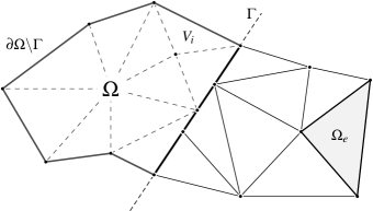
Figure 1: The two domains 1 and 2 are modelled with different methods, coupled through the interface $\Gamma$. The meshes from both sides are not necessarily consistent.

The system considered (see figure 1) is composed of two media (denoted 1 and 2) sharing an interface $\Gamma$. For every point along $\Gamma$, relations between the physical fields in the surrounding media may be established. As some of the fields may vanish at the interface, as with essential boundary conditions, the term interface relations will be preferred over continuity conditions. These relations may be expressed as a matrix equation in the following general form:

$$\begin{bmatrix}\mathbf{C}_{1}(x)\end{bmatrix}\mathbf{X}_{1}(x)=\begin{bmatrix}\mathbf{C}_{2}(x)\end{bmatrix}\mathbf{X}_{2}(x),\quad\forall\,x\in\Gamma$$ (1)

where the vectors $\mathbf{X}_{i}(x)$ represent the complex amplitudes of the physical fields involved in the interface relation for each medium $i$ and in each point $x$ of $\Gamma$. The proposed coupling approach handles both different physical models and numerical schemes, hence $\mathbf{X}_{1}(x)$ and $\mathbf{X}_{2}(x)$ used to represent the media’s dynamic state may be different. The problem is well-posed if the interface relations are known and sufficient to uniquely determine the solution. From now on, the spatial dependence $x$ in the relation (1) will be omitted for conciseness.

In order to facilitate the discussion, the weak forms for FEM and DGM are presented. As the DGM is more recent, it will be presented in greater detail. Since the proposed coupling procedure is independent of the chosen discretization and interpolation schemes, these are not discussed here. The objective of this section is to introduce the boundary terms and composition of the $\mathbf{X}_{i}(x)$ vector involved for each scheme.

2.1 Finite Element Method

In this section, the FE formulation for a second order partial differential equation is presented. The problem is set on a domain $\Omega$ whose boundary $\partial\Omega$ is assumed to be sufficiently regular. The associated weak form reads:

$$\int\displaylimits_{\Omega}a(\mathbf{f},\delta\mathbf{f})~{}\mathrm{d}\Omega+\int\displaylimits_{\Omega}L(\delta\mathbf{f})~{}\mathrm{d}\Omega+\int\displaylimits_{\partial\Omega}\mathbf{b}(\partial_{x}\mathbf{f},\partial_{y}\mathbf{f})\delta\mathbf{f}~{}\mathrm{d}\Gamma=0~{},\quad\forall\delta\mathbf{f}\in\mathcal{V}$$ (2)

where $\mathbf{f}$ denotes the vector of primary variables of the weak form and $\delta\mathbf{f}$ the associated test fields. The $\mathbf{f}$ vector belongs to a Hilbert space $\mathcal{V}$ and $\delta\mathbf{f}$ to its dual. The variables in $\mathbf{f}$ are discretized over the mesh. The bilinear function $a$ models the reaction of the media in the volume and depends on the fields and their spatial derivatives. When the weak form is discretized and written as a linear system, $a$ provides the system matrix. The inner volume forces acting on the medium are given by $L$.

The interface relations are introduced through the function $\mathbf{b}$, representing the interface relations through combinations of the so-called secondary variables. Together with the primary variables $\mathbf{b}$ forms the $\mathbf{X}$ vector used in (1).

As an example, a common choice for a fluid medium uses the scalar acoustic pressure $p$ as primary variable and the normal velocity as secondary. Hence:

$$\mathbf{X}_{1}=\begin{Bmatrix}\mathbf{b}\left(\partial_{x}\mathbf{f},\partial_{y}\mathbf{f}\right)\\ \mathbf{f}\end{Bmatrix}=\begin{Bmatrix}\left(\dfrac{\nabla p\cdot\mathbf{n}}{j\rho\omega}\right)\\ p\end{Bmatrix}$$ (3)

with $\rho$ denoting the medium’s density and $\nabla\bullet\cdot\mathbf{n}$ the normal derivative.

2.2 Discontinuous Galerkin Method

To formulate the DGM a common first step is to express the dynamic behaviour as a system of first order differential equations and then proceed towards a spatially discretized weak form [10]. The problem is then modelled by:

$$j\omega\mathbf{S}+[\mathbf{A}]\partial_{x}\mathbf{S}+[\mathbf{B}]\partial_{y}\mathbf{S}=\mathbf{0}$$ (4)

where $\mathbf{S}$, usually called state vector, is a vector whose components are combinations of the physical fields from $\mathbf{f}$ and their space derivatives. Different expressions for $\mathbf{S}$, $[\mathbf{A}]$ and $[\mathbf{B}]$ can be used [10, 16]. As an example, for a fluid medium, the following state vector will be used:

$$\mathbf{S}=\Big{\{}v_{x},~{}v_{y},~{}p\Big{\}}^{T}$$ (5)

A key aspect of the DGM is that fields are approximated as continuous-per-element and only the flux continuity is enforced across the elements. To use this approach, the domain has to be meshed and the weak form to be decomposed over it. A set of elementary sub-domains $\Omega_{e}$ (with $e=1,\ldots,N$) is then introduced and the weak form distributed over the union of all $\Omega_{e}$.

$$\sum_{e=1}^{N}\int\displaylimits_{\Omega_{e}}\mathbf{T}_{e}^{T}\Big{(}j\omega+[\mathbf{A}_{e}]\partial_{x}+[\mathbf{B}_{e}]\partial_{y}\Big{)}\mathbf{S}_{e}~{}~{}\mathrm{d}\Omega=0,\quad\forall\mathbf{T}_{e}\in\mathcal{S}_{e}$$ (6)

where $\mathbf{S}_{e}$ and $\mathbf{T}_{e}$ correspond respectively to the state variables and test functions over the element $\Omega_{e}$. The vector of unknowns, $\mathbf{S}_{e}$, is identical to the state vector previously introduced. The vector of test functions, on the other hand, belong to an Hilbert space $\mathcal{S}_{e}$, constructed as the product of Sobolev spaces in which lie the different physical fields descriptors.

In order to separate out boundary and interior terms, the following identity may be used:

$$\int\displaylimits_{\Omega_{e}}\nabla\cdot\begin{Bmatrix}\mathbf{T}_{e}^{T}[\mathbf{A}_{e}]\mathbf{S}_{e}\vspace{5pt}\\ \mathbf{T}_{e}^{T}[\mathbf{B}_{e}]\mathbf{S}_{e}\end{Bmatrix}~{}\mathrm{d}\Omega=\int\displaylimits_{\partial\Omega_{e}}\begin{Bmatrix}\mathbf{T}_{e}^{T}[\mathbf{A}_{e}]\mathbf{S}_{e}\vspace{5pt}\\ \mathbf{T}_{e}^{T}[\mathbf{B}_{e}]\mathbf{S}_{e}\end{Bmatrix}\cdot\mathbf{n}~{}\mathrm{d}\Gamma$$ (7)

with the vector $\mathbf{n}$ is the normal to $\partial\Omega_{e}$ pointing outwards $\Omega_{e}$. When evaluating (7), the derivatives related to $\mathbf{S}_{e}$ may be eliminated using (6), leading to:

$$\sum_{e=1}^{N}\int\displaylimits_{\Omega_{e}}\Big{(}j\omega\mathbf{T}_{e}-[\mathbf{A}_{e}]^{T}\partial_{x}\mathbf{T}_{e}-[\mathbf{B}_{e}]^{T}\partial_{y}\mathbf{T}_{e}\Big{)}^{T}\mathbf{S}_{e}~{}\mathrm{d}\Omega+\sum_{e=1}^{N}\int\displaylimits_{\partial\Omega_{e}}\mathbf{T}_{e}^{T}[\mathbf{F}_{e}]\mathbf{S}_{e}~{}\mathrm{d}\Gamma=0,\quad\forall\mathbf{T}_{e}\in\mathcal{S}_{e}$$ (8)

with $[\mathbf{F}_{e}]=[\mathbf{A}_{e}]n_{x}+[\mathbf{B}_{e}]n_{y}$, being the flux matrix associated with direction $\mathbf{n}=\{n_{x},~{}n_{y}\}^{T}$.

The final step towards the derivation of the DGM equation is to eliminate the volume integral in (8). This is achieved by choosing the test functions among the solutions to the adjoint of (4). Thus, taking $\mathbf{T}_{e}$ in a subspace $\mathcal{T}_{e}\subset\mathcal{S}_{e}$ such as:

$$\mathcal{T}_{e}=\Big{\{}\mathbf{T}_{e}\in\mathcal{S}_{e}\,\Big{|}\,j\omega\mathbf{T}_{e}-[\mathbf{A}_{e}]^{T}\partial_{x}\mathbf{T}_{e}-[\mathbf{B}_{e}]^{T}\partial_{y}\mathbf{T}_{e}=\mathbf{0}\Big{\}}$$ (9)

allows for the volume integrals of (8) to be cancelled, leaving only a sum of integrals over the element boundaries:

$$\sum_{e=1}^{N}\int\displaylimits_{\partial\Omega_{e}}\mathbf{T}_{e}^{T}[\mathbf{F}_{e}]\mathbf{S}_{e}~{}\mathrm{d}\Gamma=0~{},\qquad\forall\mathbf{T}_{e}\in\mathcal{T}_{e}$$ (10)

Equation (10) addresses both internal interfaces of the DGM domain and its external boundaries. The part of this equation treating with internal interfaces might be rewritten as a sum on those by introducing $\Gamma_{ee^{\prime}}$, interface between the element $e$ and $e^{\prime}$:

$$\sum_{e,e^{\prime}<e}\int_{\Gamma_{ee^{\prime}}}\mathbf{T}_{e}^{T}[\mathbf{F}_{e}]\mathbf{S}_{e}+\mathbf{T}_{e^{\prime}}^{T}[\mathbf{F}_{e^{\prime}}]\mathbf{S}_{e^{\prime}}~{}\mathrm{d}\Gamma$$ (11)

A basic requirement for the present formulation to be conservative is that the normal fluxes from both sides of $\Gamma_{ee^{\prime}}$ equal at the interface:

$$[\mathbf{F}_{e}]\mathbf{S}_{e}+[\mathbf{F}_{e^{\prime}}]\mathbf{S}_{e^{\prime}}=0$$ (12)

No condition on the $\mathbf{S}_{e}$ and $\mathbf{S}_{e^{\prime}}$ vectors has been set to enforce this condition. To this end, a numerical flux $\mathbf{f}_{ee^{\prime}}(\mathbf{S}_{e},\mathbf{S}_{e^{\prime}})$ might be constructed as proposed in the literature, e.g. [10, 16]. This flux is then split into incoming and outgoing parts and the former is used to express the latter.

On the other hand, a set of external boundaries comes to complete the formulation and reads:

$$\sum_{e}\int_{\partial\Omega_{e}\cap\partial\Omega}\mathbf{T}_{e}^{T}[\mathbf{F}_{e}]\mathbf{S}_{e}~{}\mathrm{d}\Gamma$$ (13)

The coupling procedure aims at proposing a new form for the flux $[\mathbf{F}_{e}]\mathbf{S}_{e}$ between the DGM and the FEM domains to substitute in the relevant terms of the summation (13).

3 Coupling

To establish the coupling between the weak forms, the sum of the weak forms  (2) and  (10) leads to:

$$\int\displaylimits_{\Omega}a(\mathbf{f},\mathbf{\delta f})~{}\mathrm{d}\Omega+\int\displaylimits_{\Omega}L(\mathbf{\delta f})~{}\mathrm{d}\Omega+\sum_{e=1}^{N}\int\displaylimits_{\partial\Omega_{e}\backslash\Gamma}\mathbf{T}_{e}^{T}[\mathbf{F}_{e}]\mathbf{S}_{e}~{}\mathrm{d}\Gamma+\int\displaylimits_{\partial\Omega\backslash\Gamma}\mathbf{b}\left(\partial_{x}\mathbf{f},\partial_{y}\mathbf{f}\right)\mathbf{\delta f}~{}\mathrm{d}\Gamma$$

$$+\int\displaylimits_{\Gamma}\mathbf{b}\left(\partial_{x}\mathbf{f},\partial_{y}\mathbf{f}\right)\mathbf{\delta f}~{}\mathrm{d}\Gamma+\sum_{e=1}^{N^{\prime}}\int\displaylimits_{\Gamma}\mathbf{T}_{e}^{T}[\mathbf{F}_{e}]\mathbf{S}_{e}~{}\mathrm{d}\Gamma=0~{},\quad\forall\mathbf{\delta f}\in\mathcal{V},\mathbf{T}_{e}\in\mathcal{T}_{e}$$ (14)

where the integrals corresponding to the interface between the two sub-domains are evaluated along $\Gamma$ and the rest of the section is focused on these terms.

Figure 2: Renumbering the different segments of the interface $\Gamma$ with $\Gamma_{k}$ and $k$ from $1$ to $N_{k}$. This new scheme verifies $\bigcup_{k_{=}1}^{N_{k}}\Gamma_{k}=\Gamma$.

Both domains require some form of meshing to be applied and the interface will thus be represented twice, however these meshes need not to be compatible. The union of these two discretizations splits $\Gamma$ into several segments. To express the coupling terms, an efficient way of addressing each segment of $\Gamma$ is needed. As shown in figure 2, each of the $N_{k}$ segments of $\Gamma$ connecting two consecutive nodes is denoted $\Gamma_{k}$ with $1\leq k\leq N_{k}$. This set is built in such a way that it covers the whole $\Gamma$ interface:

$$\Gamma=\bigcup_{k=1}^{N_{k}}~{}\Gamma_{k}$$

All segments have their normal oriented outwards from the DG domain. For each them, it is straightforward to identify the surrounding FEM and DGM elements, hence the element indices are omitted in the following for improved readability. The second line of (14) can then be rewritten as:

$$I_{C}=\sum_{k=1}^{N_{k}}\bigg{(}\int\displaylimits_{\Gamma_{k}}\mathbf{b}\left(\partial_{x}\mathbf{f},\partial_{y}\mathbf{f}\right)\mathbf{\delta f}~{}\mathrm{d}\Gamma+\int\displaylimits_{\Gamma_{k}}\mathbf{T}^{T}[\mathbf{F}]\mathbf{S}~{}\mathrm{d}\Gamma\bigg{)}$$ (15)

The key idea behind the proposed method is to derive explicit, local expressions for $\mathbf{b}$ and the flux $[\mathbf{F}]\mathbf{S}$ as functions of the primary variables and the state vector $\mathbf{S}$. The starting point to derive such relations is obtained from a substitution of (3) into (1) thus expressing physical continuity conditions between the DGM state vector and the FEM variables ($\mathbf{f}$ and $\mathbf{b}$):

$$[\mathbf{C}_{1}]\begin{Bmatrix}\mathbf{b}\left(\partial_{x}\mathbf{f},\partial_{y}\mathbf{f}\right)\\ \mathbf{f}\end{Bmatrix}=[\mathbf{C}_{2}]\mathbf{S}$$ (16)

where $[\mathbf{C}_{1}]$ and $[\mathbf{C}_{2}]$ are matrices combining the different quantities to represents valid interface relations.

The flux entering the DGM sub-domain is separated from the one leaving it by introducing the characteristics of the differential operator.

Given that the eigenspace of $[\mathbf{F}]$ is identical to the space of characteristics, the decomposition into outgoing and incoming flux may be obtained by diagonalizing the flux matrix: $[\mathbf{F}]=[\mathbf{P}][\mathbf{\Lambda}][\mathbf{Q}]$. In this relation $[\mathbf{P}]$ represents the matrix of eigenvectors and $[\mathbf{Q}]$ its inverse. The eigenvalues (on the diagonal of $[\mathbf{\Lambda}]$) can then be separated in two sets. The positive (resp. strictly negative) ones, associated with characteristics going out of the element (resp. entering in to) are denoted with a $+$ (resp. $-$). It is important to stress that the zero-valued characteristics are non propagative and that they will have no role in rewriting the interface relations. Despite this, for consistency, they are kept and grouped together with the positive ones. This leads to the following partitioning of the matrices $[\mathbf{P}]$ and $[\mathbf{Q}]$:

$$[\mathbf{P}]=\left[\,[\mathbf{P}^{-}]\,|\,[\mathbf{P}^{+}]\,\right],\qquad[\mathbf{Q}]=\begin{bmatrix}[\mathbf{Q}^{-}]\\ [\mathbf{Q}^{+}]\end{bmatrix},$$ (17)

with the following decomposition for the State vector $\mathbf{S}_{e}:$

$$\mathbf{S}=[\mathbf{P}^{-}]\mathbf{S}^{-}+[\mathbf{P}^{+}]\mathbf{S}^{+},\qquad\mathbf{S}^{-}=[\mathbf{Q}^{-}]\mathbf{S},\qquad\mathbf{S}^{+}=[\mathbf{Q}^{+}]\mathbf{S}$$ (18)

where $\mathbf{S}^{-}$ and $\mathbf{S}^{+}$ are the generalized coordinates of $\mathbf{S}$ in the space of characteristics, forming an intermediate step towards determining flux compliant with the boundary conditions. Introducing $\mathbf{S}^{-}$ and $\mathbf{S}^{+}$ into (16), and partitioning $[\mathbf{C}_{1}]$ into sub-matrices related to primary or secondary variables:

$$\Big{[}~{}[\mathbf{C}^{\mathbf{b}}_{1}]~{}\Big{|}~{}[\mathbf{C}^{f}_{1}]~{}\Big{]}\begin{Bmatrix}\mathbf{b}\left(\partial_{x}\mathbf{f},\partial_{y}\mathbf{f}\right)\\ \mathbf{f}\end{Bmatrix}=\Big{[}~{}[\mathbf{C}_{2}][\mathbf{P}^{-}]~{}\Big{|}~{}[\mathbf{C}_{2}][\mathbf{P}^{+}]~{}\Big{]}\begin{Bmatrix}\mathbf{S}^{-}\\ \mathbf{S}^{+}\end{Bmatrix}$$ (19)

Re-arranging this equation in order to gather terms related to $\mathbf{b}$ and $\mathbf{S}^{-}$ on one side and $\mathbf{f}$ and $\mathbf{S}^{+}$ on the other side:

$$\Big{[}~{}[\mathbf{C}^{\mathbf{b}}_{1}]~{}\Big{|}~{}-[\mathbf{C}_{2}][\mathbf{P}^{-}]~{}\Big{]}\begin{Bmatrix}\mathbf{b}\left(\partial_{x}\mathbf{f},\partial_{y}\mathbf{f}\right)\\ \mathbf{S}^{-}\end{Bmatrix}=\Big{[}~{}-[\mathbf{C}^{f}_{1}]~{}\Big{|}~{}[\mathbf{C}_{2}][\mathbf{P}^{+}]~{}\Big{]}\begin{Bmatrix}\mathbf{f}\\ \mathbf{S}^{+}\end{Bmatrix}$$ (20)

Finally, after inverting the matrix at the left hand side:

$$\begin{Bmatrix}\mathbf{b}\left(\partial_{x}\mathbf{f},\partial_{y}\mathbf{f}\right)\\ \mathbf{S}^{-}\end{Bmatrix}=\Big{[}~{}[\mathbf{C}^{\mathbf{b}}_{1}]~{}\Big{|}~{}-[\mathbf{C}_{2}][\mathbf{P}^{-}]~{}\Big{]}^{-1}\Big{[}~{}-[\mathbf{C}^{f}_{1}]~{}\Big{|}~{}[\mathbf{C}_{2}][\mathbf{P}^{+}]~{}\Big{]}\begin{Bmatrix}\mathbf{f}\\ \mathbf{S}^{+}\end{Bmatrix}$$ (21)

For convenience, the matrix linking the vectors of variables is called reflection matrix and denoted $[\mathbf{R}]$. It is partitioned into four blocks numbered $[\mathbf{R}_{ij}]$ which all link two components of the left and right hand vectors of (21):

$$[\mathbf{R}]=\Big{[}~{}[\mathbf{C}^{\mathbf{b}}_{1}]~{}\Big{|}~{}-[\mathbf{C}_{2}][\mathbf{P}^{-}]~{}\Big{]}^{-1}\Big{[}~{}-[\mathbf{C}^{f}_{1}]~{}\Big{|}~{}[\mathbf{C}_{2}][\mathbf{P}^{+}]~{}\Big{]}=\Bigg{[}\begin{matrix}[\mathbf{R}_{11}]&[\mathbf{R}_{12}]\\ [\mathbf{R}_{21}]&[\mathbf{R}_{22}]\end{matrix}\Bigg{]}$$ (22)

To assess the existence of $[\mathbf{R}]$, one can check that the dimensions of $[\mathbf{P}^{-}]$, $[\mathbf{C}_{2}]$ and $[\mathbf{C}^{b}_{1}]$ make the second matrix of (22) square. As the well-posedness is well-posed this matrix has to be full rank, thus invertible.

Using (18), a new expression for $\mathbf{b}\left(\partial_{x}\mathbf{f},\partial_{y}\mathbf{f}\right)$ taking into account the interface conditions is formed. This expression shows explicit dependence on $\mathbf{f}$ and $\mathbf{S}$, and thus are the objectives set forth in this paper accomplished.

$$\mathbf{b}\left(\partial_{x}\mathbf{f},\partial_{y}\mathbf{f}\right)=[\mathbf{R}_{11}]\mathbf{f}+[\mathbf{R}_{12}][\mathbf{Q}^{+}]\mathbf{S}$$ (23)

Based on the results obtained above, it is possible to modify the DGM flux $[\mathbf{F}]\mathbf{S}$ following the same decomposition approach. Introducing  (18) to separate incoming and outgoing characteristics, as well as  (21) and (22):

$$[\mathbf{F}]\mathbf{S}= [\mathbf{F}]\Big{(}[\mathbf{P}^{-}]\mathbf{S}^{-}+[\mathbf{P}^{+}]\mathbf{S}^{+}\Big{)}$$

$$[\mathbf{F}][\mathbf{P}^{-}][\mathbf{R}_{21}]\mathbf{f}+[\mathbf{F}]\Big{(}[\mathbf{P}^{-}][\mathbf{R}_{22}]+[\mathbf{P}^{+}]\Big{)}[\mathbf{Q}^{+}]\mathbf{S}$$ (24)

Finally, combining (23) and (24) for all the segments $\Gamma_{k}$ a new form for the coupling operator across $\Gamma$ emerges:

$$I_{C}=\sum_{k=1}^{N_{k}} \Bigg{(}\int\displaylimits_{\Gamma_{k}}\mathbf{\delta f}[\mathbf{R}_{11}]\mathbf{f}~{}\mathrm{d}\Gamma+\int\displaylimits_{\Gamma_{k}}\mathbf{\delta f}[\mathbf{R}_{12}][\mathbf{Q}^{+}]\mathbf{S}~{}\mathrm{d}\Gamma$$

$$+\int\displaylimits_{\Gamma_{k}}\mathbf{T}^{T}[\mathbf{F}][\mathbf{P}^{-}][\mathbf{R}_{21}]\mathbf{f}~{}\mathrm{d}\Gamma+\int\displaylimits_{\Gamma_{k}}\mathbf{T}^{T}[\mathbf{F}]\Big{(}[\mathbf{P}^{-}][\mathbf{R}_{22}]+[\mathbf{P}^{+}]\Big{)}[\mathbf{Q}^{+}]\mathbf{S}~{}\mathrm{d}\Gamma\Bigg{)}$$ (25)

This new operator accounts for the interface conditions (16) using only variables already present in the weak forms, enforcing the transmission of quantities across $\Gamma$ without introducing additional variables such as e.g. Lagrange multipliers. The coupling of the sub-domains is mainly provided through the second and third terms of (25) with boundary reactions in the form of the first and fourth terms.

3.1 Application to a fluid-fluid case

In order to give a better understanding of the method, this section focuses on an analytical acoustic example. The reflection matrix is deduced for fluid media and the method’s consistency is demonstrated on a simple example.

The example involve two fluid media whose physical properties are $(\rho_{i},c_{i}),~{}i\in\{1,2\}$ with $\rho_{i}$ the density of medium $i$ and $c_{i}$ its associated sound speed. The characteristic impedance for the medium $i$ is expressed as $Z_{i}=\rho_{i}c_{i}$.

The first domain (subscripted $1$) is modelled by FEM, therefore the field of representation used is the pressure $p$ and the boundary operator is described using the normal velocity as proposed in equation (3):

$$\mathbf{b}(\partial_{x}p_{1},\partial_{y}p_{1})=-\frac{\nabla p_{1}\cdot\mathbf{n}}{j\omega\rho_{1}}=\mathbf{v_{1}}\cdot\mathbf{n}$$ (26)

In the other fluid medium (subscripted $2$), DGM is used and the state vector chosen is: $\mathbf{S}_{2}=\{v_{x2},~{}v_{y2},~{}p_{2}\}^{T}$. One can then deduce the two matrices $[\mathbf{A}_{2}]$, $[\mathbf{B}_{2}]$ representing the conservation equations:

$$[\mathbf{A}_{2}]=\begin{bmatrix}0&0&\nicefrac{{1}}{{\rho_{2}}}\\ 0&0&0\\ \rho_{2}c_{2}^{2}&0&0\end{bmatrix}~{},\qquad[\mathbf{B}_{2}]=\begin{bmatrix}0&0&0\\ 0&0&\nicefrac{{1}}{{\rho_{2}}}\\ 0&\rho_{2}c_{2}^{2}&0\end{bmatrix}$$ (27)

In order to evaluate the reflection matrix $[\mathbf{R}]$, one needs to decompose the state vector in terms of characteristics. The flux matrix $[\mathbf{F}_{2}]=[\mathbf{A}_{2}]n_{x}+[\mathbf{B}_{2}]n_{y}$ is then computed and diagonalized to extract the characteristics. The two eigenvectors $[\mathbf{P}_{2}^{-}]$ and $[\mathbf{P}_{2}^{+}]$ associated with the phase speeds $c_{2}$ and $-c_{2}$ are then retrieved:

$$[\mathbf{P}_{2}^{-}]=\begin{Bmatrix}-n_{x}\\ -n_{y}\\ Z_{2}\end{Bmatrix}~{},\,[\mathbf{P}_{2}^{+}]=\begin{bmatrix}{n_{x}}&{-n_{y}}\\ {n_{y}}&{n_{x}}\\ {Z_{2}}&{0}\end{bmatrix}~{},$$

$$[\mathbf{Q}_{2}^{-}]=\begin{bmatrix}-\dfrac{n_{x}}{2}&-\dfrac{n_{y}}{2}&\dfrac{1}{2Z_{2}}\end{bmatrix},\,[\mathbf{Q}_{2}^{+}]=\begin{bmatrix}\dfrac{n_{x}}{2}&\dfrac{n_{y}}{2}&\dfrac{1}{2Z_{2}}\\ {-n_{y}}&n_{x}&0\end{bmatrix}$$ (28)

The reflection matrix consists mainly in a particular rewriting of continuity conditions. For a fluid/fluid interface, interface relations enforce continuity of pressure and normal veclocity which leads to the following form of (16):

$$\begin{Bmatrix}\mathbf{b}(\partial_{x}p_{1},\partial_{y}p_{1})\\ p_{1}\end{Bmatrix}=\begin{bmatrix}n_{x}&n_{y}&0\\ 0&0&1\end{bmatrix}\begin{Bmatrix}v_{x2}\\ v_{y2}\\ p_{2}\end{Bmatrix}$$ (29)

As proposed in the current work, $\mathbf{S}_{2}$ is replaced by its representation in the space of characteristics see  (18). Reordering the terms leads to:

$$\begin{bmatrix}1&1\\ 0&-Z_{2}\end{bmatrix}\begin{Bmatrix}\mathbf{b}(\partial_{x}p_{1},\partial_{y}p_{1})\\ \mathbf{S}_{2}^{-}\end{Bmatrix}=\begin{bmatrix}0&1&0\\ -1&Z_{2}&0\end{bmatrix}\begin{Bmatrix}p_{1}\\ \mathbf{S}_{2}^{+}\end{Bmatrix}$$ (30)

Solving for $\mathbf{b}$ and $\mathbf{S}_{2}$, the explicit fluid-fluid reflection matrix is obtained as:

$$[\mathbf{R}]=\begin{bmatrix}-1/Z_{2}&2&0\\ 1/Z_{2}&-1&0\end{bmatrix}$$ (31)

In this matrix, the last null column corresponds to the null-valued characteristics which are, by definition, non-propagative and are not transmitted through the coupling interface. The coefficients of $[\mathbf{R}]$ are generally difficult to analyze (since they couple two very different approaches). The consistency of the form derived may be checked through the diagonal terms. For a fluid-fluid coupling, the first diagonal term corresponds to the ratio of acoustic velocity and pressure and fits with the definition of acoustic impedance: $Z=p/v$. Finally, the second diagonal term makes sense in the DGM framework since it forces the incoming and outgoing characteristics to propagate in opposite directions.

3.2 Remarks on discretization and choice of shape functions

Equation (9) sets a requirement on the set of trial functions without actually proposing an expression for them. In the present work, following  [10], the test functions are chosen to be in the form of plane waves. Thus, they are composed as a superposition of $N_{w}$ plane waves whose directions are distributed in the unit disc . Using this interpolation, the $\mathbf{S}$ vector on each element is expanded as:

$$\mathbf{S}=\sum_{n=1}^{N_{w}}a_{n}\mathbf{U}_{n}e^{-j\mathbf{k}_{n}\cdot(\mathbf{r}-\mathbf{r}_{c})}$$ (32)

with $\mathbf{r}_{c}$ mapping to the center of the element and $\mathbf{k}_{n}$ and are the wave numbers of the different plane waves. The $\mathbf{U}_{n}$ vector acts in a fashion similar to that of polarization vectors, relating the propagating term to certain quantities of the state vector. Finally, the set of the different $a_{n}$ for all the elements are the amplitude factors and components of the solution vector. Using such an interpolation strategy for the state vector, the method is called DGM with plane waves (PWDGM). A more in-depth explanation is given in reference [10].

Figure 3: Example of recontruction basis for PWDGM with $N_{w}=8$. The tilt of the basis with respect to the $x$ axis is controled by $\delta\theta$

As a finite number $N_{w}$ of plane waves is distributed on the unit disc, as shown in figure 3, one can easily understand it induces privileged directions. Each time the solution’s direction of propagation coincides with one of the waves of the basis, one expects the error to drop. The reconstruction of waves whose directions are situated between two waves of the basis is challenging. A way to ensure a good approximation for all directions is to use a $N_{w}$ sufficiently large, reducing the distance between two waves and introducing more directions where error drops (privileged). A second possibility is to tilt the wave basis using $\delta\theta$ and align one of the wave with the solution’s direction of propagation. This can be done independently from the other elements’ basis but finding a good algorithm to predict the best tilt is not a trivial task. Another way to address this precision loss is to use more elements, disposed so to avoid patterns in the mesh and take advantage of the inter-element compensation [16]. The main limit to this approach then comes from the lower bound in element size: as the solution is reconstructed by superposing plane waves, they must be given enough space between their origin (center of element) and the boundaries to combine.

On the other hand, the usual way to interpolate fields in the scope of FEM makes use of polynomials. The edges of the mesh are augmented of $p+1$ nodes (including both ends) used for a $p$-order approximation. Different basis have been proposed over the years. For the examples that follow, quadratic Lagrange polynomials were used.

In the light of the previous considerations, it is clear that all the integral terms from (25) require numerical integration of polynomials and/or exponentials. When the integrals only involve exponentials or polynomials, as for the first and last terms, one can use a fully analytical integration. Even if possibly cumbersome to write, the numerical evaluation of the integral will then be as precise as the machine itself and computationally efficient.

Nevertheless, when considering integrals involving products of polynomials and exponentials (as do the second and third terms of (25)), the integration scheme’s performance is critical. Proposing an efficient numerical integration of products of polynomials and exponentials is not trivial. Complex exponentials and polynomials tends to oscillate at different scales, rendering difficult the choice of a integration technique. Finally the large number of integration points required to get a proper value tends to slow down the resolution: indeed, the integration is triggered twice per coupling segment. Some improvements in the medium-high frequency range may be accessible through a change of integration technique or pre-computing.

4 Application and results

To validate the proposed coupling approach as well as to demonstrate its performance, some test cases are presented in this section. The first two provide insights into the convergence and dispersion properties and an existing analytical solution is used as a reference. The quality of the results is evaluated through $\mathcal{L}_{2}$ relative error:

$$\epsilon=\bigg{(}\frac{\int_{\Omega}\left|p-p_{ref}\right|^{2}~{}\mathrm{d}\Omega}{\int_{\Omega}\left|p_{ref}\right|^{2}~{}\mathrm{d}\Omega}\bigg{)}^{1/2}$$ (33)

where $p$ corresponds to the predicted pressure and $p_{ref}$ to the analytical reference. The third example deals with a more complex geometry and aims at demonstrating the hybrid method with incompatible meshes, acute corners, rounded shape and a relatively large domain. In all simulations air medium at 20°C is used with the following properties:

$$\rho=1.213~{}\mathrm{kg}\cdot\mathrm{m}^{-1},\qquad c=341.973~{}\mathrm{m}\cdot\mathrm{s}^{-1}$$ (34)

In the examples, $\delta\theta$ is always null except otherwise stated.

4.1 Dispersion analysis

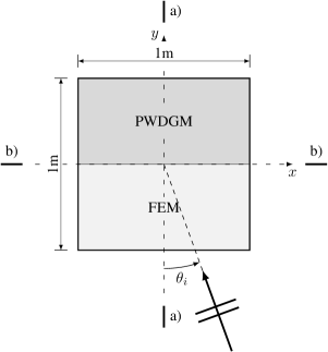
Figure 4: The domain used for the dispersion analysis, a $1$m square with the plane wave field imposed on all sides at an angle $\theta_{i}$. Positions a) and b) are of special interest.

For the dispersion analysis a square domain with 1 m side length is used, see figure 4. The purpose is to demonstrate the numerical behaviour of the proposed coupling approach. The excitation is in the form of a plane wave imposed on the boundary of the square, the wave front propagating at an angle $\theta_{i}$ from the lower $y$ axis.

In figure 4, two different angles of particular interest are identified as a) and b). The former corresponds to a wave entering through the boundary of one of the sub-domains only, implying that the error builds up sequentially in one sub-domain first and then the other. For directions marked b) the incident field is parallel to the coupling boundary and there is no flux across the interface for the reference solution.

A pure PWDGM solution is also computed with the purpose of providing a numerical result which is independent of the proposed coupling approach. This solution is computed for the same mesh and approximation order as used in the PWDGM part of the coupled model.

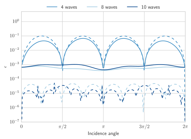
Figure 5: Evolution of the relative error with respect to the incidence angle of a plane wave over a 1m square domain. Half the domain is modelled with DGM and the rest with FEM. Triangular elements are used on both sides, dashed lines are for the pure DGM reference and $f=1000$ Hz. (Color online)

From a theoretical point of view, the FEM part of the solution is not sensitive to the angle of incidence and the error as a function of $\theta_{i}$ should be constant. In practice, the mesh may have an influence, introducing privileged directions where the error may build up but this is generally negligible. The solution obtained using only PWDGM for the square problem exhibits $N_{w}$ arches over the $[0,~{}2\pi]$ range of incidence angle. This solution is referred to as the pure PWDGM reference in figure 5. The observed arches are well known in the literature, and stem from the privileged directions induced by the waves used in the base (see section 3.2 and figure 3). However, as the number of waves is increased the error related to these is reduced, see figure 5.

In figure 5, the results for the coupled FEM-DGM solution at $f=1000$ Hz are shown. With 4 waves per element, the archs discussed above appear in the solution, but are not observed for the higher number of waves, $N_{w}=8$ and $N_{w}=10$. The error seems to be controlled by the FEM solution, as the overall accuracy for this coupled solution is about two orders of magnitude worse than the pure PWDGM solution. Furthermore, the error levels for $N_{w}=8$ and $N_{w}=10$ and above are close to each other, indicating that the FEM is limiting the accuracy in this case and this observation is confirmed by a direction-independent error around $10^{-3}$.

To investigate this further the error generated in the FEM and PWDGM domains separately is shown in figure 6 for $Nw\in\{4,10\}$.

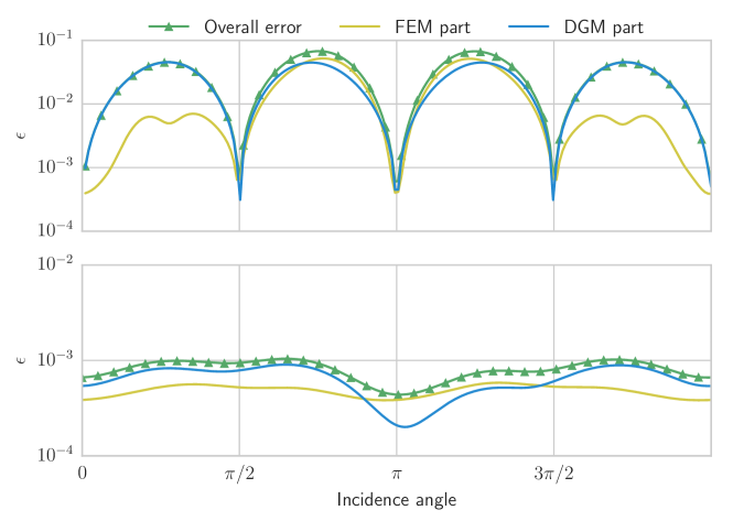
Figure 6: Contribution of the two different schemes to the global error with respect to the incidence angles for $f=1000$ Hz and $N_{w}=4$ (top) or $N_{w}=10$ (bottom). (Color Online)

For $N_{w}=4$, the PWDGM-related error is dominating over the whole range. Between $\theta_{i}=\pi/2$ rad and $\theta_{i}=3\pi/2$ rad, where the error is generated first in the PWDGM domain before being transmitted to the FEM and both methods then exhibit the same error profile. When comparing with the error in the FEM domain for the other half of the range (wave coming from the FEM side), one can see that the PWDGM archs are actually preponderant in shaping the error profile. For this first case, the hybrid method has an error level similar to that of the pure PWDGM reference.

For $N_{w}=10$, while figure 5 shows that PWDGM is not limiting the accuracy, the different contributions at the bottom of figure 6, suggests that both methods contribute more or less with equal shares in the error generation.

This apparent contradiction is related to the large difference of precision between a 10 wave PWDGM and FEM for the coupled system. As figure 5 suggests that the PWDGM should be accurate enough and the error thus has its origin in the FEM part with its lower resolution in the model used. The error is dominated by phase error building in the FEM which in the coupling to the PWDGM pollutes the PWDGM solution for these particular directions of incidence.

4.2 Kundt’s tube

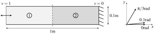
Figure 7: A simple 1$\times$0.1m Kundt tube used as a benchmark. The two labeled regions are modelled with FEM or PWDGM. On the right, the first wave of the basis used for figures 8 to 10.

In this second example, the proposed coupling method is used to predict the pressure field in a rigid, rectangular cavity excited by a unit velocity at one end, see figure 7. This cavity has dimensions 1 m$\times$0.1 m and is divided into two sub-domains with a interface at the middle of the tube. The purpose is to assess the DGM sensitivity to the wave base, here through varying the tilt angle of the base as shown in figures 3 and 7.

To assess the hybrid model’s convergence rate, a baseline case with the whole domain modelled with FEM is used. This is shown as the black dashed line in figure  8. In the numerical tests performed with the hybrid model one of the sub-domains is modelled by FEM and the other by PWDGM. Initial checks with excitation applied at both ends did not reveal any noticeable difference, thus only results for an excitation applied on the FEM side are included here.

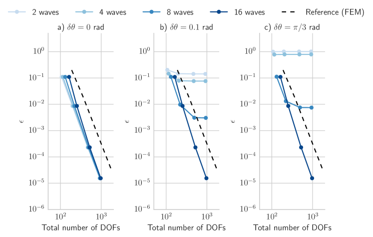
Figure 8: Evolution of the relative $\mathcal{L}_{2}$ error with respect to the the size of the linear system for $f=1000$ Hz. The dashed line is a reference for which the all domain was modelled using FEM ; other lines are for different $N_{w}$. (Color online)

This two first tests aim at testing the two classical refinement approaches for FEM and PWDGM on the hybrid model. The first of the tests uses a classical FEM strategy by gradually refining the FE side mesh without modifying the PWDGM parameters. The analysis conducted for different numbers of waves $N_{w}$ in the reconstruction basis and different tilt angles $\delta\theta$. The refinement of the FE sub-domain is the same as the on used to compute the baseline (dashed black line) shown in figure 8. Each of the three graphs is computed for a noticeable tilt $\delta\theta$ of the wave basis. Indeed, for a long, merely 1D, acoustic cavity, keeping one wave aligned with the main axis of the cavity seems beneficial. In order to understand this behaviour, the properties of the interpolation strategy for the PWDGM as explained in section 3.2 are useful. For example, figure 8a is obtained for a highly favourable PWDGM configuration. Since an even number of waves $N_{w}$ is considered, $N_{w}/2$ pairs corresponding to the two propagation directions of the solution (forward & backward) are present and one of them aligned with the solution direction. This allows to decrease considerably the reconstruction error in the PWDGM domain, down to machine precision. In this case, no error should be generated by the PWDGM and only the FEM sub-domain and coupling have an impact. In figure 8.a), the convergence rate of the hybrid method for all numbers of waves in the basis is comparable to that of the pure FE baseline (black dashed line). This first result indicates that the coupling itself is not negatively contributing to the error.

For the two last parts of figure 8, a saturation of the error rate can be observed, even on figure 8b where the tilt angle is small. This behaviour complies with the PWDGM effect previously discusssed. When the FE part of the hybrid scheme reaches at a sufficently high refinement factor, the PWDGM error can become the highest and the overall error doesn’t drop any further when adding elements in the FEM domain. The main difference between graphs 8b and 8c is to be seen for $N_{w}\in\{2,4\}$ compared to $N_{w}=8$. Indeed for small a number of waves tilting the basis has a dramatic impact (resulting in 100% error rate) whereas the other waves compensate the precision loss when there are sufficiently many in the base ($N_{w}=8$ here).

Finally, the error for $N_{w}=16$ stays the same for all tilt angles $\delta\theta$. An explanation for it is to be found in the relative error levels for the FEM and PWDGM domains. Adding waves to the basis tends to reduce the maximum error in PWDGM  [10, 16] and, once a given $N_{w}$ is reached, the PWDGM error does not exceed the FEM error anymore. For $N_{w}=16$, the PWDGM error is systematically lower than the FEM error which then dominates regardless of the orientation of the solution with the PWDGM reconstruction basis. As the FEM solution is not sensitive to the tilt of the wave basis, the convergence curve is not impacted either and the hybrid scheme converges at the same rate as the FEM for all $\delta\theta$.

Keeping the number of waves $N_{w}$ constant and varying the FE mesh, and vice versa, the influence of the tilt angle $\delta\theta$ on the error in the hybrid solution may be studied. For a fixed FE mesh, and varying of the number of waves in the base, the results shown in figure 9 where $\delta\theta$ varies between $0$ and $\pi$, are obtained. The tilt angles used in the previous results, $\delta\theta=0.1$ rad and $\delta\theta=\pi/3$ rad, are marked in the figure. Results for different $N_{w}$ are presented in figure 9 with 2 superimposed black dashed lines for $\delta\theta=0.1$ rad and $\delta\theta=\pi/3$ rad. The results from the hybrid method (solid lines) are compared with their pure PWDGM counterparts (dashed lines with matching color). The results confirm the previous observations in the current paper and are consistent with previously published research,  [16]. The PWDGM error is at its lowest whenever a wave of the basis is aligned with the solution. This is observed for both the pure PWDGM baseline references and the coupled solutions. For the latter though, the peak error is lower as a consequence of the error build-up mechanisms in a PWDGM domain.

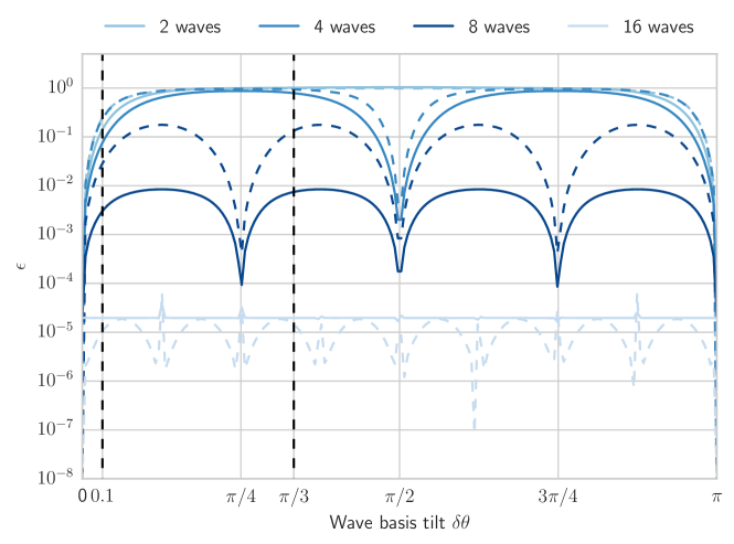
Figure 9: Evolution of the relative error with respect to the tilt angle $\delta\theta$ for different numbers of waves and a given refinement of the FE mesh at $f=1000$ Hz. Dashed lines are the corresponding full DGM reference. The two vertical dashed lines mark the two angles used on figure 8. (Color online)

For a fixed number of waves $N_{w}$, the influence of the mesh refinement is shown in figure 10. Three different refinements of the FE mesh (baseline and 10 or 15% increase in number of degrees of freedom) are shown as function of $\delta\theta$. This graph shows that replacing half of the domain by a FE model allowed to reduce the maximum error. On the other end, it also suggests than if the added FEM is not precise enough, it tends to prevent the error drops introduced by PWDGM.

Figure 10: Evolution of the relative error with respect to the tilt angle $\delta\theta$ for a given number of waves but different refinements of the FE mesh (the lighter the more refined). The graph was generated at $f=1000$ Hz and the black line is a pure DGM reference. (Color online)

To add some background to this phenomenon, one could go back to the PWDGM solution as such. The PWDGM establishes a flux through the boundaries of the elements and the associated errors are related to the quality of the reconstruction of the flux at these boundaries. If half the domain is replaced by another (potentially more precise) method, then part of the DG error cannot build up and the global error ends up capped to a lower rate. For $N_{w}=8$ in figure 9, the effect is particularly prominent, a full PWDGM solution gives a $10^{-1}$ peak error but coupling to FE allows to drop down by one order of magnitude.

4.3 Open resonant cavity with tight corner

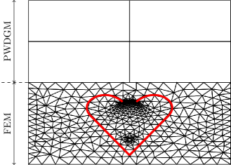
Figure 11: Example of mixed mesh with an incompatible coupling interface.

To demonstrate the applicability of the proposed coupling approach, a hybrid solution of a slightly more complex geometrical arrangement is used. A 1 meter-square cavity is filled with air and an open resonant rigid body is placed inside. The lower part, containing the resonator, is modelled using FEM in order to accurately account for all the geometrical details. As an example, the sharp angle at the lowest part of the rigid body makes the field inside hard to resolve using plane waves. In addition, the top part is modelled using 4 PWDGM elements, see figure 11, with a base of 32 plane waves per element.

Two different cases are tested. First, a point source is placed at the bottom of the resonator and excites the volume through a unit velocity at $f=52$ Hz. The resulting pressure field for this case is shown in figure 12(a). The second test case uses an unit velocity excitation from the top of the cavity, at $f=260$ Hz. The pressure map for the second example is shown in figure 12(b). In both figures, the dashed red line marks the interface $\Gamma$ between the two sub-domains, each modelled using the two different discretization methods, coupled using the approach discussed in the present paper. For both studied case, the naive replacement of half the FEM domain by a PWDGM one led to a 15% decrease of the number of degrees of freedom in the final linear system.

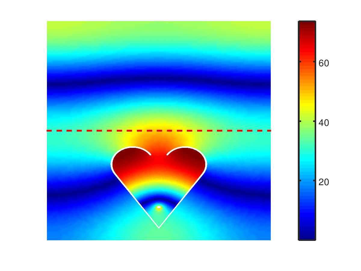
(a) Excitation by a point source placed
near the bottom corner of the resonator with $f=52$ Hz.

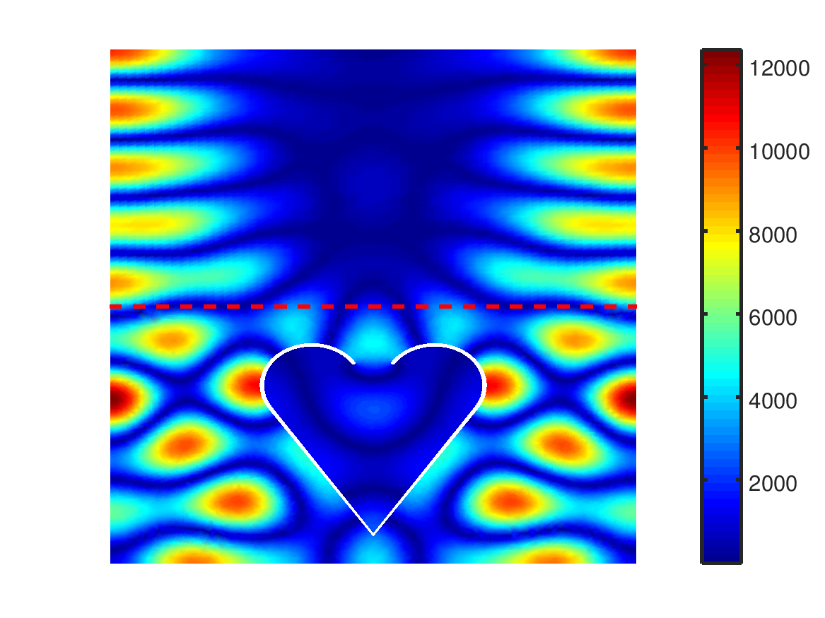
(b) Excitation by a unit velocity from the top,
rigid boundary with $f=260$ Hz.

Figure 12: Simulation of the pressure field for two different excitations. Compared to the one presented as an example in figure 11, only the FEM domain’s refinement is increased. The dashed line symbolizes the coupling interface.

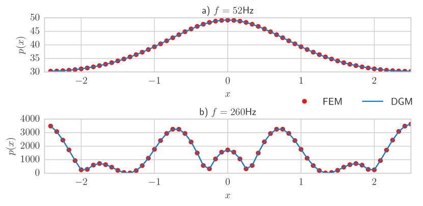
Figure 13: Pressure profiles along the interface between the method as seen by the FE and PWDG schemes. (Color online)

As may be seen from figure 12(b), the pressure solutions is visually continuous with no artefacts generated close to the coupling interface. Thus, the pressure field, generated in the FE domain seems correctly transmitted to the PWDGM domain and the cavity modes seem to be reconstructed correctly in both sub-domains despite the coarse PWDGM mesh. As part of the investigations made, a converged pure FEM resolution produced the same results. Interestingly, for the higher frequency excitation, the coarse DGM mesh captures the lobes well.

In order to demonstrate that the continuity between the pressure at the interface between the sub-domains is fulfilled, the pressure along $\Gamma$ as computed by each of the two methods is shown in figure 13. For the first case, one clearly sees that the central lobe, due the resonator’s radiation, is approximated the same way from both sides. For the second one, the same pressure profile is computed even if many modes are spread across the boundary. These results confirm the validity of the proposed coupling approach.

5 Conclusion

This work proposes an effective coupling strategy for the Finite-Element Method and the Discontinuous Galerkin with Plane Waves. The resulting hybrid scheme is based on a reflection matrix that maps FEM’s physical field and DGM’s characteristics seamlessly. This procedure presents several advantages, the first of which being to enforce a discrepancy-free coupling. The coupling then relies on continuity conditions between state vectors that are straightforward to write for most pairs of media. The litterature on FEM adaptations of physical models is abundant (even for complex media as in [17]) and extensions the PWDGM approach has been proposed [16] recently.

After presenting the coupling and an analytical derivation for a simple case, numerical examples were provided. First an set of academic examples were used to support the claim of a incidence angle-independant coupling, methods specificities conservation and simulation ability. Both methods limits were explored in the scope of the coupled approach in these first examples and it was made clear how this approach could be used optimally in a third one.

The last use case showed how FEM could be used to protect resonant features or geometrical details and embed them in a larger PWDGM domain. The good adaptativity of the first method was combined to the large-scale modelling properties of the second to reduce model complexity without precision loss.

References

- [1] Marburg S. Six boundary elements per wavelength: Is that enough? Journal of Computational Acoustics 2002; 10(01):25–51.
- [2] Babuška I, Melenk J. The Partition of Unity Method. International Journal for Numerical Methods in Engineering Feb 1997; 40(4):727–758.
- [3] Babuška I, Banerjee U, Osborn JE. Generalized finite element methods — main ideas, results and perspective. International Journal of Computational Methods 2004; 1(01):67–103.
- [4] Bériot H, Gabard G, Perrey-Debain E. Analysis of high-order finite elements for convected wave propagation. International journal for numerical methods in engineering 2013; 96(11):665–688.
- [5] Bériot H, Prinn A, Gabard G. Efficient implementation of high-order finite elements for Helmholtz problems. International Journal for Numerical Methods in Engineering Apr 2016; 106(3):213–240, doi:10.1002/nme.5172.
- [6] Ladevèze P. A new computational approach for structure vibrations in the meidum frequency range. Comptes Rendus de l’Académie des Sciences 1996; 322:849–856.
- [7] Riou H, Ladevèze P, Kovalevsky L. The Variational Theory of Complex Rays: An answer to the resolution of mid-frequency 3D engineering problems. Journal of Sound and Vibration Apr 2013; 332(8):1947–1960, doi:10.1016/j.jsv.2012.05.037.
- [8] Desmet W. A wave based prediction technique for coupled vibro-acoustic analysis. Phd, Katholieke Universteit Leuven, Leuven, Belgium Dec 1998.
- [9] Deckers E, Atak O, Coox L, D’Amico R, Devriendt H, Jonckheere S, Koo K, Pluymers B, Vandepitte D, Desmet W. The wave based method: An overview of 15 years of research. Wave Motion 2014; 51(4):550–565.
- [10] Gabard G. Discontinuous Galerkin methods with plane waves for time-harmonic problems. Journal of Computational Physics Aug 2007; 225(2):1961–1984, doi:10.1016/j.jcp.2007.02.030.
- [11] Gabard G, Gamallo P, Huttunen T. A comparison of wave-based discontinuous Galerkin, ultra-weak and least-square methods for wave problems. International Journal for Numerical Methods in Engineering Jan 2011; 85(3):380–402, doi:10.1002/nme.2979.
- [12] van Hal B, Vanmaele C, Desmet W, Silar P, H-H P. Hybrid finite element — wave based method for steady-state acoustic analysis. Proceedings of ISMA2004, Leuven, Belgium, 2004; 1629–1642.
- [13] Lee JS, Deckers E, Jonckheere S, Desmet W, Kim YY. A direct hybrid finite element–wave based modelling technique for efficient analysis of poroelastic materials in steady-state acoustic problems. Computer Methods in Applied Mechanics and Engineering Jun 2016; 304:55–80, doi:10.1016/j.cma.2016.02.006.
- [14] Ladevèze P, Riou H. On Trefftz and weak Trefftz discontinuous Galerkin approaches for medium-frequency acoustics. Computer Methods in Applied Mechanics and Engineering Aug 2014; 278:729–743, doi:10.1016/j.cma.2014.05.024.
- [15] Dazel O, Gaborit M, Gabard G. Couplage entre la MEF et la DGM avec ondes planes pour l’acoustique. S04 Nouveaux Résultats et Modèles En Interaction Fluide-Structure, AFM, Association Française de Mécanique: Lyon, France, 2015.
- [16] Gabard G, Dazel O. A discontinuous Galerkin method with plane waves for sound absorbing materials. International Journal for Numerical Methods in Engineering 2015; .
- [17] Atalla N, Hamdi MA, Panneton R. Enhanced weak integral formulation for the mixed (u,p) poroelastic equations. The Journal of the Acoustical Society of America 2001; 109(6):3065, doi:10.1121/1.1365423.