Kinetic Energy and Angular Momentum of Free Particles in the Gyratonic pp-Waves Space-times

Gyratonic pp-waves are exact solutions of Einstein’s equations that represent non-linear gravitational waves endowed with angular momentum. We consider gyratonic pp-waves that travel in the $z$ direction and whose time dependence on the variable $u={1\over\sqrt{2}}(z-t)$ is given by gaussians, so that the waves represent short bursts of gravitational radiation propagating in the $z$ direction. We evaluate numerically the geodesics and velocities of free particles in the space-time of these waves, and find that after the passage of the waves both the kinetic energy and the angular momentum per unit mass of the particles are changed. Therefore there is a transfer of energy and angular momentum between the gravitational field and the free particles, so that the final values of the energy and angular momentum of the free particles may be smaller or larger in magnitude than the initial values.

PACS numbers: 04.20.-q, 04.20.Cv, 04.30.-w

(1) wadih@unb.br, jwmaluf@gmail.com

(2) rocha@fis.unb.br

(3) sc.ulhoa@gmail.com

(4) fernandolessa45@gmail.com

1 Introduction

The field equations of the theory of general relativity admit a class of exact solutions that represent non-linear plane gravitational waves. These solutions are known as the Kundt family of space-times [1], and were thoroughly studied by Ehlers and Kundt [2, 3]. They may describe short bursts of gravitational radiation. The idea is that far from the source we may approximate a realistic gravitational wave by an exact plane wave. Some of these non-linear plane waves are vacuum solutions of Einstein’s equations, and are idealized manifestations of the gravitational field, in similarity to the source-free wave solutions of Maxwell’s equations, which are excellent descriptions of realistic monochromatic plane electromagnetic waves. Ehlers and Kundt [2, 3] asserted that the vacuum pp-waves (parallelly propagated plane-fronted waves) are geodesicaly complete (see Ref. [4]), and also showed that one may add the amplitudes of two pp-waves running in the same direction, in which case the principle of linear superposition holds (section 2-5.3 of Ref. [2]). They argue that this fact indicates a striking analogy with Maxwell’s theory.

Penrose [5] also investigated these waves, and concluded that “it is fair to assume that they (the non-linear gravitational waves) are no less physical (as idealizations) than their flat space couterparts”, although he also concluded that is not possible to imbed these waves globally in any hyperbolic pseudo-Euclidean space. The difficulty, according to Penrose, is that the total (gravitational) energy of such plane waves is infinite. However, the same feature takes place for idealized waves in flat space. It must be noted that the pp-waves do not imply or lead to the violation of any physical principle or physical property. They are ordinary manifestations of the theory.

Gyratonic pp-waves represent the exterior gravitational field of a spinning source that propagates at the speed of light. The exterior space-time of a localized spinning source, that moves at the speed of light, was first studied by Bonnor [6], later by Griffiths [7], and rediscovered by Frolov and collaborators [8, 9, 10, 11], who attempted to relate this space-time with the model of spinning particles, the “gyratons”. The gyratonic pp-waves were recently investigated by Podolský, Steinbauer and Švarc [12]. These authors studied several properties of the non-linear waves, such as the impulsive limit, the geodesic motion, and also emphasized the role of the off-diagonal components in the line element, that is described in terms of Brinkmann coordinates [13]. The gyratonic pp-waves are non-linear gravitational waves endowed with angular momentum.

In this article we evaluate the geodesics and velocities of free particles in the space-time of gyratonic pp-waves, by means of a numerical analysis, and show that there is not only a transfer of energy between the free particles and the gravitational wave [14], but also a transfer of angular momentum. Both transfers of energy and angular momentum between the particles and the field take place locally, i.e. in the regions where the particles are located. This is an argument in favour of the localization of gravitational energy. It does not seem reasonable to consider that a local variation of energy of a free particle is related to the instantaneous variation of the total gravitational energy, evaluated at spacelike (or null) infinity, for instance. We note that Ehlers and Kundt already investigated the action of a pp-wave on free particles initially at rest, and concluded that after the passage of the wave, the particles acquire velocities, both transverse and longitudinal to the wave (see section 2-5.8 of [2]). We show in this article, as in Ref. [14], that the final energy of the particles may be smaller than the initial energy.

In section 2 we describe the gyratonic pp-waves, according to the presentation of Ref. [12]. The graphic results are presented in section 3, and the final comments in section 4.

2 Gyratonic pp-waves

The study of the gyratonic pp-waves emerged from the investigation by Bonnor [6] and by Griffiths [7] of the interior and exterior fields of a spinning “null fluid”, which is a configuration that travels at the speed of light. A review of this issue is given in section 18.5 of Ref. [15]. In the following we will adopt the presentation of Ref. [12]. We will consider a wave that travels along the $z$ direction. The gyratonic source $(\varrho,j_{i})$ is localized along the axis $x=y=0$, or in the immediate neighbourhood around this axis. The energy-momentum of the source is prescribed by the radiation density $T_{uu}=\varrho$, and by the terms $T_{ui}=j_{i}$ that represent the spinning character of the source. The line element is given in terms of Brinkmann coordinates [13], with an off-diagonal term. It is given by [12]

$$ds^{2}=d\rho^{2}+\rho^{2}d\phi^{2}+2\,dudv-2J\,dud\phi+H\,du^{2}\,.$$ (1)

The integration of the field equations in the vacuum region, outside the matter source, imply that the functions $H=H(u,\rho,\phi)$ and $J=J(u,\rho,\phi)$ are periodic in $\phi$. The general form of these functions is [12]

$$J=\omega(u)\rho^{2}+\chi(u,\phi)\,,$$ (2)

$$H=\omega^{2}(u)\rho^{2}+2\omega(u)\chi(u,\phi)+H_{0}(u,\rho,\phi)\,,$$ (3)

where $\omega(u)$ and $\chi(u,\phi)$ are arbitrary functions of $u$ and $(u,\phi)$, respectively. If $\chi$ is taken to be independent of the angular coordinate $\phi$, i.e., if $\chi=\chi(u)$, then the function $H_{0}$ must only satisfy the equation

$$\nabla^{2}H_{0}=\biggl{(}{{\partial^{2}}\over{\partial x^{2}}}+{{\partial^{2}}\over{\partial y^{2}}}\biggr{)}H_{0}=0\,.$$ (4)

We will adopt this simplification in the considerations below.

In flat space-time, the variables $u$ and $v$ are related to the ordinary time variable $t$ and to the usual cylindrical coordinate $z$ according to

$$u={1\over{\sqrt{2}}}(z-t)\,,$$ (5)

$$v={1\over{\sqrt{2}}}(z+t)\,.$$ (6)

We use the relations above to carry out a coordinate transformation of the metric tensor, from the $(u,\rho,\phi,v)$ coordinates to $(u,\rho,\phi,z)$ coordinates, so that the line element is rewritten as

$$ds^{2}=(H-2)du^{2}+d\rho^{2}+\rho^{2}d\phi^{2}+2\sqrt{2}\,dudz-2J\,dud\phi\,.$$ (7)

The flat space-time is obtained if we make $H=J=0$. From the metric tensor above we obtain, by means of the standard procedure, the Lagrangian for a free particle of mass $m$ that travels along geodesics labelled by an affine parameter $\lambda$. The Lagrangian is given by

$$L=\frac{m}{2}\left[(H-2)\dot{u}^{2}+\dot{\rho}^{2}+\rho^{2}\dot{\phi}^{2}+\sqrt{8}\,\dot{u}\dot{z}-2J\,\dot{u}\dot{\phi}\right]\,,$$ (8)

where the dot represents variation with respect to $\lambda$.

By solving the equations of motion we find, in similarity to the analysis of Ref. [14], that ${d\,}^{2}u/d\lambda^{2}=0$. As a consequence we may set $\dot{u}=1$, and thus we take the coordinate $u$ as the affine parameter along the geodesic. In this way, the set of geodesic equations read

$$\ddot{\rho}+\partial_{\rho}J\dot{\phi}-\rho\dot{\phi}^{2}-\frac{1}{2}\partial_{\rho}H = 0\,,$$ (9)

$$\ddot{\phi}+\frac{2}{\rho}\dot{\rho}\dot{\phi}-\frac{\partial_{\rho}J}{\rho^{2}}\dot{\rho}-{1\over{2\rho^{2}}}\biggr{[}2\partial_{u}J+\partial_{\phi}H\biggl{]} = 0\,,$$ (10)

$$\ddot{z}+{1\over{\sqrt{2}\rho^{2}}}\biggr{[}\rho^{2}\partial_{\rho}H-J\partial_{\rho}J\biggl{]}\dot{\rho}-\frac{\partial_{\phi}J}{\sqrt{2}}\dot{\phi}^{2}+\frac{\partial_{\phi}H}{\sqrt{2}}\dot{\phi}$$

$$+{1\over{\sqrt{2}\rho}}\biggl{[}{2J-\rho\partial_{\rho}J}\biggr{]}\dot{\rho}\dot{\phi}+{1\over{\sqrt{8}\rho^{2}}}\biggl{[}{\rho^{2}\partial_{u}H-J(\partial_{\phi}H+2\partial_{u}J)}\biggr{]} = 0\,.$$ (11)

These equations are equivalent to the geodesic equations given by Eq. (75) of Ref. [12], presented in the $(\rho,\phi,v)$ coordinates.

The function $\omega(u)$ is related to a rigid rotation of the space-time, and can be removed by a gauge transformation [12]. Without loss of generality, we can make $\omega=0$. Therefore, the remaining arbitrary functions are

$$J=\chi(u)\,,$$ (12)

$$H=H_{0}(u,\rho,\phi)\,.$$ (13)

The $u$-dependence of these two functions will be given by gaussians, that represent short bursts of gravitational waves. We already discussed in Ref. [14] that in order to obtain qualitative features of the geodesic equations, it makes no difference whether we use gaussians or derivatives of gaussians. We note that in the analysis of the gravitational memory effect carried out in Ref. [16], use is made of the first, second and third derivatives of gaussians. The advantage of using the second derivative is that it dispenses a multiplicative dimensional constant in the metric tensor components [14]. By requiring $J=0$, we obtain the pp-wave considered in Refs. [14, 16].

As for the $(x,y)$ or $(\rho,\phi)$ (where $x=\rho\cos\phi$ and $y=\rho\sin\phi$) dependence of the function $H_{0}$, that must satisfy Eq. (4), we will establish two possibilities. The first one is the $\times$ polarization. It reads

$$H_{0}=\frac{1}{2}(xy)\frac{d\,^{2}}{du^{2}}(e^{-u^{2}/\sigma^{2}})\,,$$ (14)

and the function $\chi(u)$ is chosen to be

$$\chi={1\over{10}}e^{-u^{2}/\sigma^{2}}\,.$$ (15)

which also represents a burst. In the expressions above, $\sigma$ is a constant with dimension of length. The multiplicative factor $1/10$ is introduced only for graphical reasons (for adjusting the figures). For our purposes, it makes no qualitative difference whether we use the $\times$ polarization, or the $+$ polarization given by $x^{2}-y^{2}$, instead of $xy$.

The second choice of $H_{0}$ is

$$H_{0}=\frac{1}{4}[\log(\rho/\rho_{0})]\frac{d\,^{2}}{du^{2}}(e^{-u^{2}/\sigma^{2}})\,,$$ (16)

and the $\chi$ function is given by

$$\chi={1\over{10}}e^{-(0.1\,u^{2}/\sigma^{2})}\,.$$ (17)

In Eqs. (16) and (17), not only $\sigma$, but also $\rho_{0}$ is a constant with dimension of length in natural units. For simplicity, both constants will be taken to be $\sigma=\rho_{0}=1$. Except for the second derivative of the gaussian, the function in Eq. (16) corresponds to the Aichelburg-Sexl type monopole [17].

3 The geodesic of free particles

In this section we present the graphical results obtained by solving the geodesic equations (9), (10) and (11) numerically, by means of the program MATHEMATICA. We also plot the Kinetic energy per unit mass $K$ of the free particles before and after the passage of the wave (in which case the space-time is flat), as a function of the variable $u$. In view of Eq. (5), $K$ is obtained from the equation

$$4K=\dot{\rho}^{2}+\rho^{2}\dot{\phi}^{2}+\dot{z}^{2}\,,$$ (18)

where the dot represents variation with respect to $u$ (we would have $2K$ on the left hand side, if the variation were with respect to $t$).

3.1 $H_{0}$ given by equation (14)

For the initial conditions given by

$$\rho_{0}=0.3,\ \ \ \phi_{0}=0,\ \ \ z_{0}=0,\ \ \ \dot{\rho_{0}}=0,\ \ \ \dot{\phi_{0}}=0,\ \ \ \dot{z_{0}}=0.2\,,$$ (19)

for $u=0$, we obtain the geodesic behaviour displayed in Figures [1] and [2], where both coordinates (Figure [2]) and velocities (Figure [2]) are given as functions of $u$.

Figure 1: Coordinates when $H_{0}$ is given by (14) and for the initial conditions (19).

Figure 2: Velocities when $H_{0}$ is given by (14) and for the initial conditions (19).

The trajectory of the free particle in the $x-y$ plane is plotted in Figure [3]. The initial state of the particle is in the upper part of the Figure. The particle acquires angular momentum during the passage of the gravitational wave, and then resumes the inertial movement along a straight line in the lower part of the Figure. It is clear that there is a transfer of angular momentum between the wave and the free particle. An analogous behaviour has been studied also in Ref. [16], but in the context of a pp-wave with $J=0$, with the polarization $x^{2}-y^{2}$.

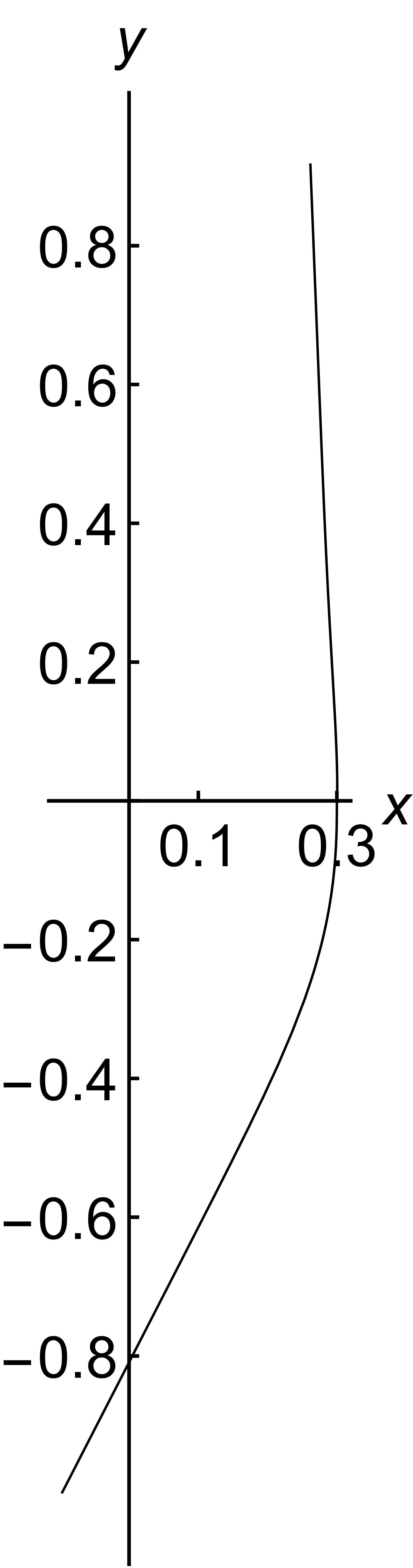
Figure 3: Trajectory in the $x-y$ plane when $H_{0}$ is given by (14) and for the initial conditions (19).

We also choose an alternative set of initial conditions,

$$\rho_{0}=0.3,\ \ \ \phi_{0}=\frac{\pi}{3},\ \ \ z_{0}=0,\ \ \ \dot{\rho_{0}}=0,\ \ \ \dot{\phi_{0}}=0,\ \ \ \dot{z_{0}}=0.2\,,$$ (20)

also for $u=0$, where the only difference with respect to initial conditions (19) is the value of the initial angle $\phi_{0}$. The reason for choosing this alternative set is to show that the behaviour of the Kinetic energy per unit mass of the free particle is highly sensitive to the initial conditions. Figure [5] displays the behaviour of the Kinetic energy by choosing the polarization given by Eq. (14), with the initial conditions (19). In Figure [5] we see the behaviour of the Kinetic energy of the particle, after the passage of the wave, when the initial conditions are given by Eq. (20).

Figure 4: Kinetic energy when $H_{0}$ is given by (14) and initial conditions (19).

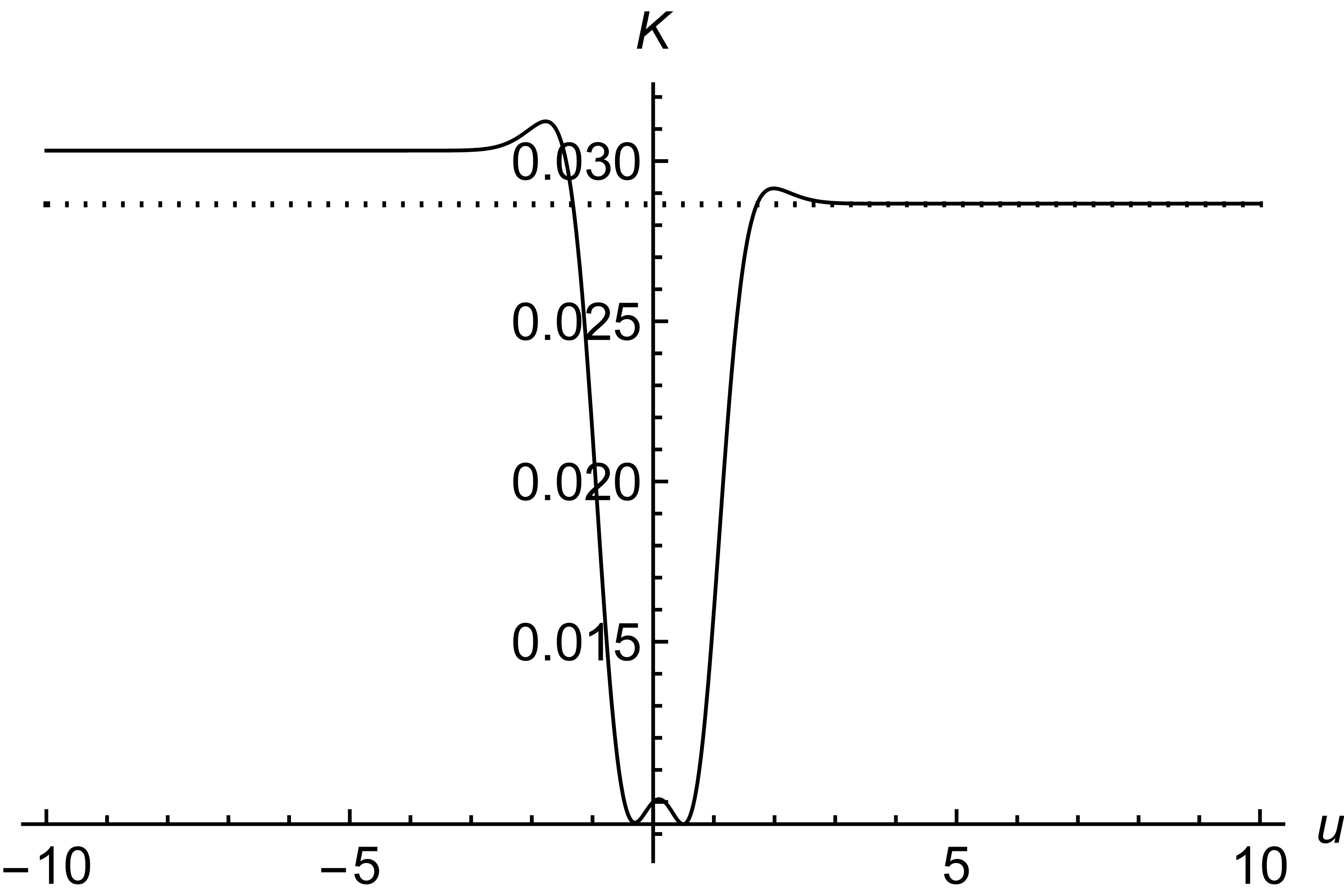
Figure 5: Kinetic energy when $H_{0}$ is given by (14) and initial conditions (20).

In view of Eq. (5), a positive variation of $u$ corresponds to a negative variation of the time coordinate $t$. Therefore, if $u$ grows from left to right in all Figures, the time coordinate $t$ grows from right to left. Thus, we see that in Figure [5] the final Kinetic energy is smaller than the initial energy, whereas in Figure [5] the final Kinetic energy is larger than the initial energy. This is exactly the behaviour discussed in Ref. [14]. The passage of a gravitational wave may either increase or decrease the energy of a free particle, and therefore there is a local transfer of energy between the particle and the wave.

In order to explore a little further the variation of the Kinetic energy, before and after the passage of the wave (but without the purpose of exhausting the investigation), we define the quantity

$$\Delta K={{K_{f}-K_{i}}\over{K_{f}+K_{i}}}\,,$$ (21)

where $K_{f}$ is the final Kinetic energy evaluated at $u=-5$, and $K_{i}$ is the initial Kinetic energy evaluated at $u=5$ ($\Delta t>0$, since $\Delta u<0$). Thus, the particle acquires or looses energy according to $\Delta K>0$ or $\Delta K<0$, respectively. Note that the gravitational wave considered here is not axially symmetric. Choosing the initial conditions (always for $u=0$),

$$\rho_{0}=0.1,\ \ \ z_{0}=0,\ \ \ \dot{\rho_{0}}=0,\ \ \ \dot{\phi_{0}}=0,\ \ \ \dot{z_{0}}=0,$$ (22)

we obtain the behaviour displayed by Figure [6], where $\Delta K$ varies with respect to $\phi_{0}$. It is possible to show that by increasing or decreasing the value of $\dot{\rho_{0}}$ around $\dot{\rho_{0}}=0$, the curve moves as a whole up or down in the Figure, respectively.

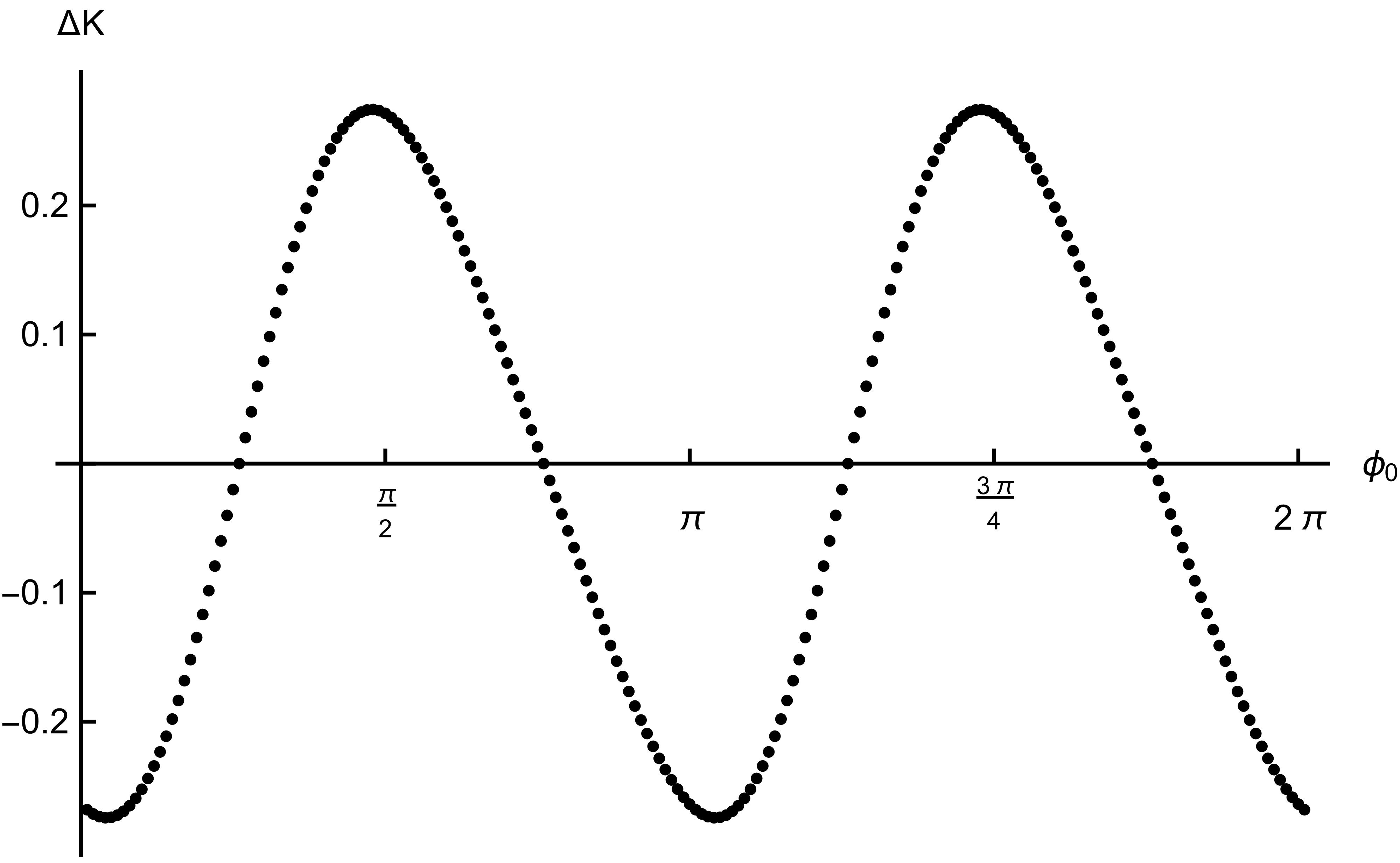
Figure 6: Variation of the Kinetic energy with respect to $\phi_{0}$, in the initial conditions $(\ref{22})$.

3.2 $H_{0}$ given by equation (16)

Let us now consider the second choice for the function $H_{0}$, given by Eq. (16), together with $\chi(u)$ given by (17). In this case, the wave is axially symmetric. The initial conditions are chosen to be

$$\rho_{0}=0.6,\ \ \ \phi_{0}=0,\ \ \ z_{0}=0,\ \ \ \dot{\rho_{0}}=0,\ \ \ \dot{\phi_{0}}=0,\ \ \ \dot{z_{0}}=0.2\,.$$ (23)

The geodesic behaviour and the velocities of a free particle under the action of the gravitational wave, for the initial conditions above, are displayed in Figures [8] and [8].

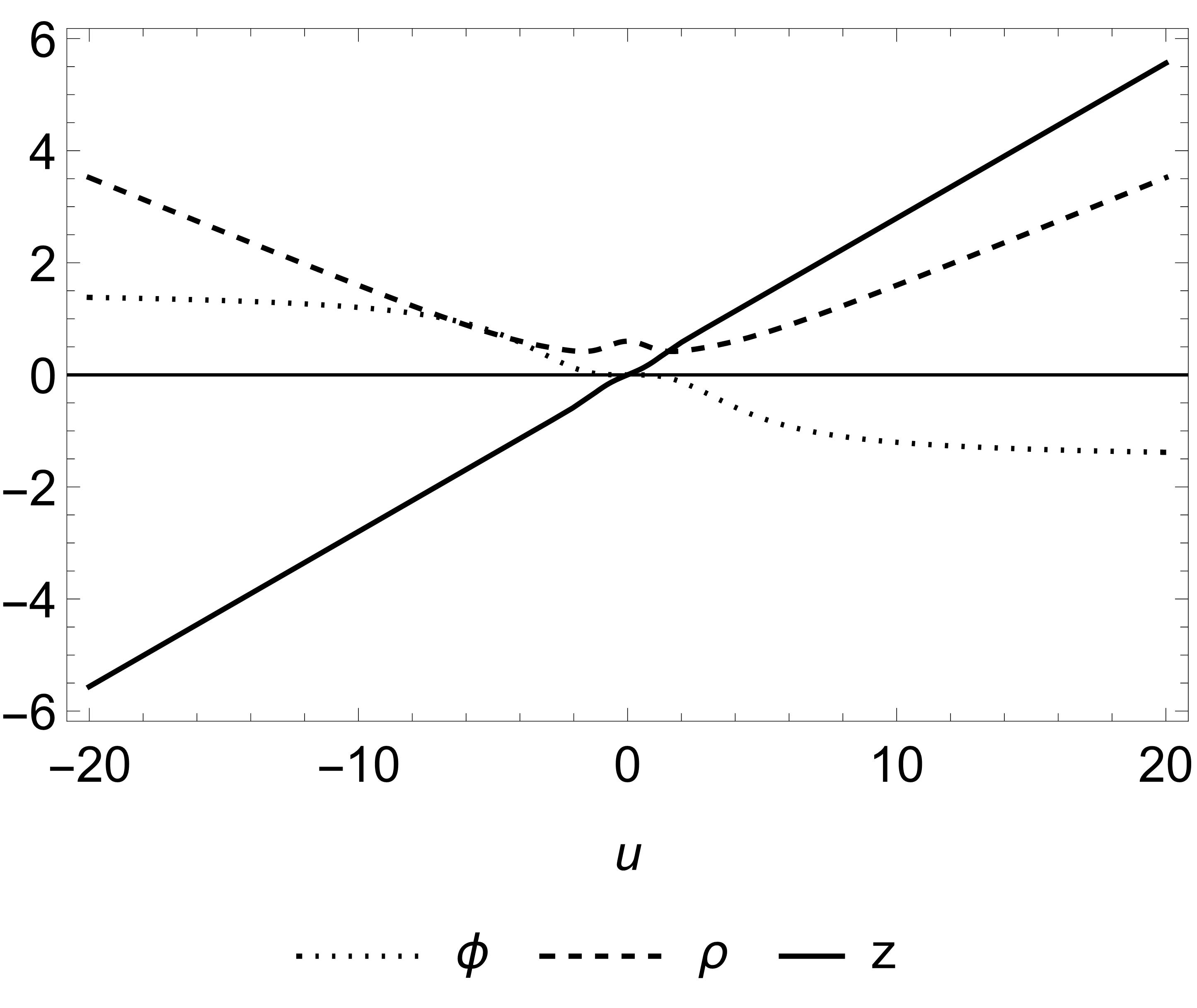
Figure 7: Coordinates when $H_{0}$ is given by (16) and for the initial conditions (23).

Figure 8: Velocities when $H_{0}$ is given by (16) and for the initial conditions (23).

The trajectory of a free particle in the $x-y$ plane is plotted in Figure [9]. Similarly to the situation displayed in Figure [3], the particle acquires angular momentum during the passage of the gravitational wave, and then resumes the inertial movement along a straight line. Both the initial and final trajectories of the particle are linear. These trajectories are in the upper and lower part of the Figure, respectively, and are almost vertical trajectories. In these regions, the particle is free and away of the gravitational field of the wave.

Figure 9: Trajectory in the $x-y$ plane when $H_{0}$ is given by (16) and for the initial conditions (23).

In the context of this gravitational wave, there also occurs a transfer of energy between the wave and the free particle. We observe here that one relevant feature is the sign of $\dot{\rho_{0}}$. Let us establish the initial conditions

$$\rho_{0}=0.6,\ \ \ \phi_{0}=0,\ \ \ z_{0}=0,\ \ \ \dot{\rho_{0}}=\pm 0.2,\ \ \ \dot{\phi_{0}}=0,\ \ \ \dot{z_{0}}=0\ .$$ (24)

For the initial conditions given above, the Kinetic energy of the particle increases or decreases after the passage of the wave, according to the sign of $\dot{\rho_{0}}$, as shown in Figures [11] and [11].

Figure 10: Increasing of the Kinetic energy for the initial conditions (24), and for positive sign of $\dot{\rho_{0}}$.

Figure 11: Decreasing of the Kinetic energy for the initial conditions (24), and for negative sign of $\dot{\rho_{0}}$.

We recall that the dot represents variation with respect to $u$. Therefore, if $\dot{\rho_{0}}>0$, the particle is initially approaching the gyratonic source. Likewise, if $\dot{\rho_{0}}<0$, the particle is initially getting away from the source. As Figures [11] ($\dot{\rho_{0}}>0$) and [11] ($\dot{\rho_{0}}<0$) indicate, the particle gain or loose energy as it approaches or gets away from the source located around the axis $z=0$.

Still in the context of $H_{0}$ given (16), we display in Figures [13] and [13] the angular momentum per unit mass of the particle with respect to $u$. The definitions in polar coordinates are

$$M_{x} = \sin{\phi}\left(\rho\dot{z}-z\dot{\rho}\right)-\rho z\dot{\phi}\cos{\phi}\,,$$

$$M_{y} = \cos{\phi}\left(z\dot{\rho}-\rho\dot{z}\right)-\rho z\dot{\phi}\sin{\phi}\,,$$

$$M_{z} = \rho^{2}\dot{\phi}\,.$$ (25)

Figure [13] is constructed taking into account initial conditions (23), whereas in Figure [13] we consider the initial conditions (24), with $\dot{\rho_{0}}>0$. The two Figures clearly show the variation of the angular momentum of the free particle caused by the gravitational wave. The quantity $M^{2}=M_{x}^{2}+M_{y}^{2}+M_{z}^{2}$ is conserved in the context of Figure [13], but not in the context of Figure [13]. This feature confirms that there is a transfer of angular momentum between the particle and the wave.

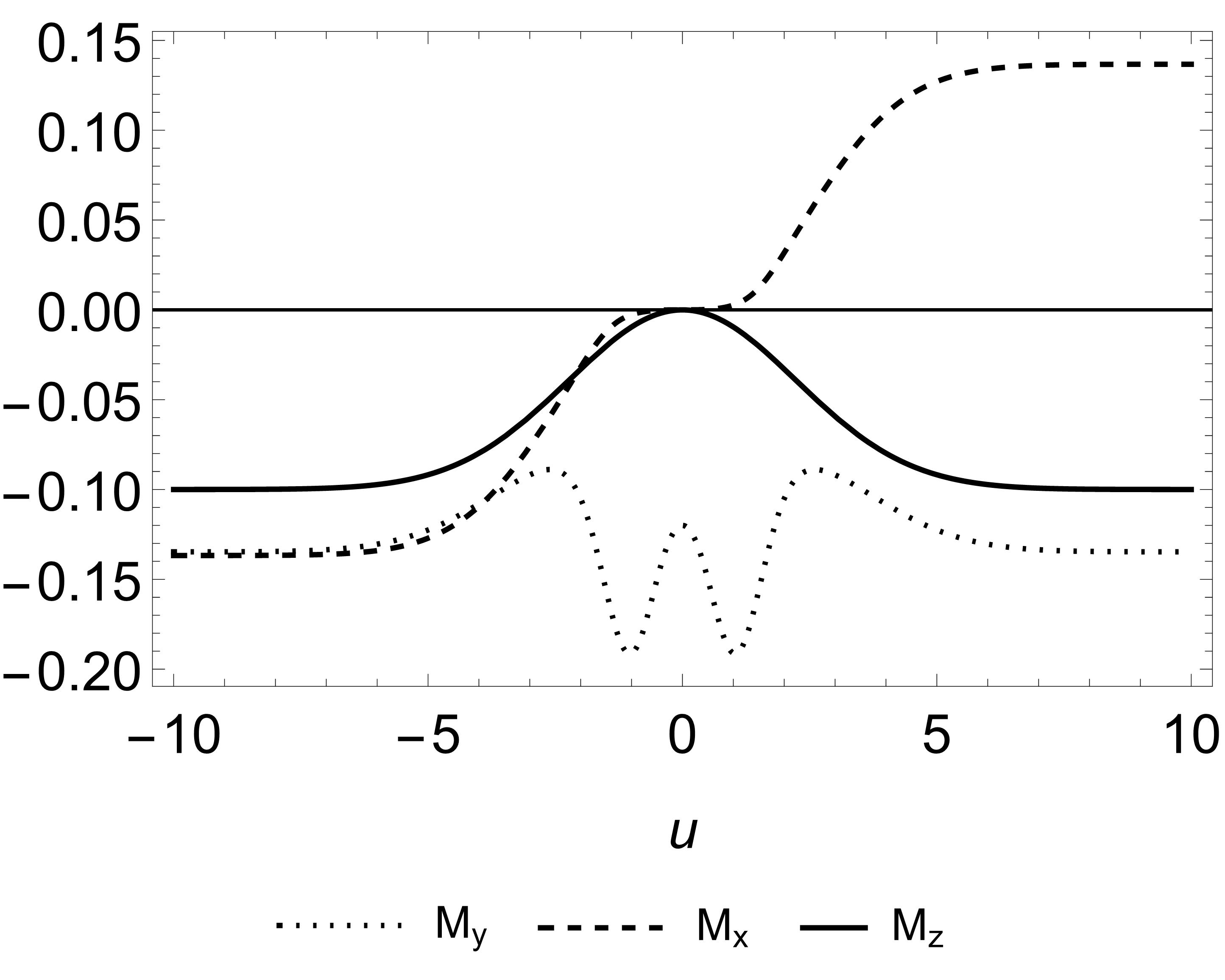
Figure 12: Angular momentum of the particle for the initial conditions (23).

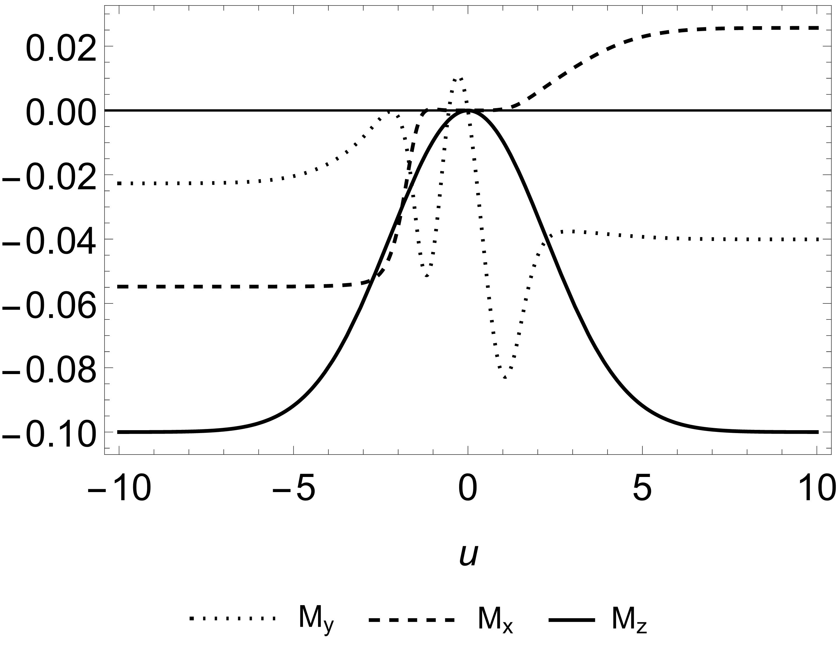
Figure 13: Angular momentum of the particle for the initial conditions (24), and $\dot{\rho_{0}}>0$.

4 Final Comments

The non-linear pp-waves, as investigated in Refs. [2, 3], are simple, elegant and natural vacuum solutions of Einstein’s equations. Although they have been studied for a quite long time, it is reasonable to say that the full physical consequences of the non-linear waves have not been investigated so far. These waves share similarities with plane monochromatic electromagnetic waves, that are source-free solutions of Maxwell’s equations, and that yield an excellent description of electromagnetic radiation. Ehlers and Kundt showed that the principle of linear superposition holds to a certain extent for pp-waves, since one may add the amplitudes of two pp-waves that travel in the same direction (Ref. [2], section 2-5.3). This fact supports the analogy between pp-waves and electromagnetic waves. Gyratonic pp-waves, on the other hand, are generated by a source that travels at the speed of light. Physically, these waves might be a realistic manifestation of the field equations. There is no physical principle or physical property that is violated by the existence of these waves. Therefore, they are legitimate manifestations of the theory of general relativity.

We have shown in this article that the Kinetic energy and the angular momentum per unit mass (also the linear momentum, but it has not been explicitly addressed here) of a free particle vary during the passage of a wave. In particular, the final Kinetic energy of a free particle might be smaller than the initial Kinetic energy. It seems clear that there is a local transfer of energy-momentum and angular momentum between the particle and the gravitational field of a wave. As a consequence, the wave may gain or loose energy as it travels in space. Ehlers and Kundt (Ref. [2], section 2-5.8) investigated the action of a pp-wave in the form of a pulse on a cloud of dust particles at rest, and concluded that the particles acquire velocities after the pulse has swept the particles. They argue that this fact suggests convincingly that a cloud or particles is able to extract energy from a gravitational wave, as supported by Bondi [18]. However, this argument applies when the free particles are initially at rest. We have seen in this article that if the free particles are not initially at rest, then the cloud of particles may transfer (positive) energy to the gravitational wave.

One interesting extension of the present analysis is the consideration of impulsive gravitational waves, as carried out, for instance, in Refs. [19, 20, 21]. The profile of an impulsive wave is obtained from a single gaussian function, which can be normalised to 1 according to the expression,

$${1\over{\sigma\sqrt{2\pi}}}\int_{-\infty}^{+\infty}du\;e^{-{(u^{2}/2\sigma^{2}})}=1\;,$$

and taking the limit $\sigma\rightarrow 0$. This limit cannot be taken in the present analysis, because we cannot introduce a dimensional amplitude in Eqs. (14, 16) (the second derivative of the gaussian is already of dimension (length)^-2), and also because the second derivative of the gaussian cannot be normalised (the integral from $-\infty$ to $+\infty$ of the latter vanishes). The analysis of the action of impulsive gravitational waves on free particles will be carried out elsewhere, and compared to the results of Refs. [19, 20, 21].

The feature discussed in the present article does not take place in the context of linearised gravitational waves, in which case the wave is supposed to be unaffected by the medium, although it becomes linearised somehow. Moreover, a gravitational wave, linearised or not, imparts a memory effect to the detector, which must involve a transfer of energy-momentum and/or angular momentum to the detector. This issue, specifically in the context of linearised gravitational waves, must be investigated and satisfactorily explained on theoretical grounds.

References

- [1] D. Kramer, H. Stephani, M. A. H. MacCallum and H. Herlt, “Exact Solutions of the Einstein’s Field Equations”, Cambridge University Press, Cambridge, (1980).
- [2] J. Ehlers and W. Kundt, “Exact Solutions of the Gravitational Field Equations”, in “Gravitation: an Introduction to Current Research”, edited by L. Witten (Wiley, New York, 1962).
- [3] P. Jordan, J. Ehlers and W. Kundt, “Republication of: Exact solutions of the field equations of the general theory of relativity”, Gen. Relativ. Grav. 41, 2191-2280 (2009).
- [4] J. L. Flores and M. Sánchez, “Ehlers-Kundt Conjecture about Gravitational Waves and Dynamical Systems”, arXiv:1706.03855
- [5] R. Penrose, “A Remarkable Property of Plane Waves in General Relativity”, Rev. Mod. Phys. 37, 215 (1965).
- [6] W. B. Bonnor, “Charge moving with the speed of light in Einstein-Maxwell theory”, Int. J. Theor. Phys. 3, 257 (1970).
- [7] J. B. Griffiths, “Some phsyical properties of neutrino-gravitational fields”, Int. J. Theor. Phys. 5, 141 (1972).
- [8] V. P. Frolov and D. V. Fursaev, “Gravitational field of a spinning radiation beam pulse in higher dimensions”, Phys. Rev. D 71, 104034 (2005).
- [9] V. P. Frolov, W. Israel and A. Zelnikov, “Gravitational field of relativistic gyratons”, Phys. Rev. D 72, 084031 (2005).
- [10] V. P. Frolov and A. Zelnikov, “Relativistic gyratons in asymptotically AdS spacetime”, Phys. Rev. D 72, 104005 (2005).
- [11] V. P. Frolov and A. Zelnikov, “Gravitational field of charged gyratons”, Class. Quantum Grav. 23, 2119 (2006).
- [12] J. Podolský, R. Steinbauer and R. Švarc, “Gyratonic pp-waves and their impulsive limit”, Phys. Rev. D. 90, 044050, (2014).
- [13] H. W. Brinkmann, “On Riemann spaces conformal to Euclidean spaces”, Proc. Natl. Acad. Sci. U.S. 9, 1 (1923); Math. Ann. 94, 119 (1925).
- [14] J. W. Maluf, J. F. da Rocha-Neto, S. C. Ulhoa and F. L. Carneiro, “Plane Gravitational Waves, the Kinetic Energy of Free Particles and the Memory Effect”, arXiv:1707.06874
- [15] J. B. Griffiths and J. Podolsky, “Exact Space-Times in Einstein’s General Relativity” (Cambridge University Press, Cambridge, 2009).
- [16] P.-M. Zhang, C. Duval, G. W. Gibbons and P. A. Hovarthy, “Soft gravitons and the memory effect for plane gravitational waves”, Phys. Rev. D 96, 064013 (2017).
- [17] P. C. Aichelburg and R. U. Sexl, “On the gravitational field of a massless particle”, Gen. Relativ. Gravit. 2, 303 (1971).
- [18] H. Bondi, “Plane gravitational waves in general relativity”, Nature, 179, 1072 (1957).
- [19] J. Podolsky, R. Svarc, R. Steinbauer and C. Sämann, “Penrose junction conditions extended: Impulsive waves with gyratons”, Phys. Rev. D 96 064043 (2017).
- [20] C. Sämann, R. Steinbauer and R. Svarc, “Completeness of general pp-waves spacetimes and their impulsive limit”, Class. Quantum Grav. 33, 215006 (2016).
- [21] J. Podolsky and K. Vesely, “New examples of sandwich gravitational waves and their impulsive limit”, Czech. J. Phys. 48, 871 (1998).