Dynamic compensation and homeostasis:
a feedback control perspective

Abstract

“Dynamic compensation” is a robustness property where a perturbed biological circuit maintains a suitable output [Karin O., Swisa A., Glaser B., Dor Y., Alon U. (2016). Mol. Syst. Biol., 12: 886]. In spite of several attempts, no fully convincing analysis seems now to be on hand. This communication suggests an explanation via “model-free control” and the corresponding “intelligent” controllers [Fliess M., Join C. (2013). Int. J. Contr., 86, 2228-2252], which are already successfully applied in many concrete situations. As a byproduct this setting provides also a slightly different presentation of homeostasis, or “exact adaptation,” where the working conditions are assumed to be “mild.” Several convincing, but academic, computer simulations are provided and discussed.

1 Introduction

In systems biology, i.e., an approach of growing importance to theoretical biology (see, e.g., Alon [2006], Klipp et al. [2016], Kremling [2012]), basic control notions, like feedback loops, are becoming more and more popular (see, e.g., Åström et al. [2008], Cowan et al. [2014], Cosentino et al. [2011], Del Vecchio et al. [2015]). This communication intends to show that a peculiar feedback loop permits to clarify the concept of dynamic compensation (DC) of biological circuits, which was recently introduced by Karin et al. [2016]. DC is a robustness property. It implies, roughly speaking, that biological systems are able of maintaining a suitable output despite environmental fluctuations. As noticed by Karin et al. [2016] such a property arises naturally in physiological systems. The DC of blood glucose, for instance, with respect to variation in insulin sensitivity and insulin secretion is obtained by controlling the functional mass of pancreatic beta cells.

The already existing and more restricted homeostasis, or exact adaptation, deals only with constant reference trajectories, i.e., setpoints. It is achievable via an integral feedback (see, e.g., Alon et al. [1999], Briat et al. [2016], Miao et al. [2011], Stelling et al. [2004], Yi et al. [2000])

Remark 1.1

PIDs (see, e.g., Åström et al. [2008], O’Dwyer [2009]) read:

$$u=K_{P}e+K_{I}\int e+K_{D}\dot{e}$$ (1)

where

• $u$, $y$, $y^{\star}$ are respectively the control and output variables, and the reference trajectory.

• $e=y-y^{\star}$ is the tracking error,

• $K_{P},K_{I},K_{D}\in\mathbb{R}$ are the tuning gains.

To the best of our knowledge, they are, strangely enough, more or less missing in the literature on theoretical biology, although they lead to the most widely used control strategies in industry.

From $K_{P}=K_{D}=0$ in Equation (1), the following integral feedback is deduced:

$$u=K_{I}\int e$$ (2)

Compare Equation (2) with the references above on homeostasis, and Somvanshi et al. [2015]. See Abouaïssa et al. [2017b], and the references therein, for an application to ramp metering on freeways in order to avoid traffic congestion.

Conditions for DC have already been investigated by several authors: Karin et al. [2017a, b], Sontag [2017], Villaverde et al. [2017]. Parameter identification, which plays a key rôle in most of those studies, leads, according to the own words of Karin et al. [2017b], to some kind of “discrepancy,” which is perhaps not yet fully cleared up. We suggest therefore another roadmap, i.e., intelligent feedback controllers as defined by Fliess et al. [2013]. Many concrete applications have already been developed all over the world. Some have been patented. The bibliography contains for obvious reasons only recent works in biotechnology: Bara et al. [2016], Join et al. [2017a], Lafont et al. [2015], MohammadRidha et al. [2018], Tebbani et al. [2016].

An unexpected byproduct is derived from Remark 1.1 and the comparison in Abouaïssa et al. [2017b] between Equation (2) and our intelligent proportional controller (Fliess et al. [2013]). Exact adaptation means now a “satisfactory” behavior thanks to the feedback loop defined by Equation (2) when the working conditions are “mild.” The result by Karin et al. [2016] via a mechanism for DC based on known hormonal circuit reactions, which states that exact adaptation does not guarantee dynamical compensation, remains therefore valid in this new context.

This exploratory research report is organized as follows. Intelligent controllers are summarized in Section 2, where the connection between classic PIs and intelligent proportional controllers is also presented. Section 3, which is hevily influenced by Abouaïssa et al. [2017b], defines dynamic compensation and exact adaptation. Section 4 displays various convincing, but academic, computer experiments. Some concluding remarks may be found in Section 5.

2 Model-free control and intelligent controllers

See Fliess et al. [2013] for full details.

2.1 Generalities

2.1.1 The ultra-local model

The poorly known global description of the plant, which is assumed for simplicity’s sake to be SISO (single-input single output), is replaced by the ultra-local model:

$$\boxed{y^{(\nu)}=F+\alpha u}$$ (3)

where:

• the control and output variables are respectively $u$ and $y$;

• the derivation order $\nu$ is often equal to $1$, sometimes to $2$; in practice $\nu\geq 3$ has never been encountered;

• the constant $\alpha\in\mathbb{R}$ is chosen by the practitioner such that $\alpha u$ and $y^{(\nu)}$ are of the same magnitude; therefore $\alpha$ does not need to be precisely estimated.

The following comments might be useful:

• Equation (3) is only valid during a short time lapse and must be continuously updated;

• $F$ is estimated via the knowledge of the control and output variables $u$ and $y$;

• $F$ subsumes not only the system structure, which most of the time will be nonlinear, but also any external disturbance.

2.1.2 Intelligent controllers

Set $\nu=2$. Close the loop with the following intelligent proportional-integral-derivative controller, or iPID,

$$u=-\frac{F-\dot{y}^{\ast}+K_{P}e+K_{I}\int e+K_{D}\dot{e}}{\alpha}$$ (4)

where:

• $e=y-y^{\star}$ is the tracking error,

• $K_{P},K_{I},K_{D}\in\mathbb{R}$ are the tuning gains.

When $K_{I}=0$, we obtain the intelligent proportional-derivative controller, or iPD,

$$u=-\frac{F-\dot{y}^{\ast}+K_{P}e+K_{D}\dot{e}}{\alpha}$$ (5)

When $\nu=1$ and $K_{I}=K_{D}=0$, we obtain the intelligent proportional controller, or iP, which is the most important one,

$$\boxed{u=-\frac{F-\dot{y}^{\ast}+K_{P}e}{\alpha}}$$ (6)

Combining Equations (3) and (6) yields:

$$\dot{e}+K_{P}e=0$$ (7)

where $F$ does not appear anymore. The tuning of $K_{P}$ is therefore straightforward.

Remark 2.1

See Join et al. [2017b] for a comment on those various controllers.

2.1.3 Estimation of $F$

Assume that $F$ in Equation (3) is “well” approximated by a piecewise constant function $F_{\text{est}}$. The estimation techniques below are borrowed from Fliess et al. [2003, 2008] and Sira-Ramírez et al. [2014]. Let us summarize two types of computations:

1. Rewrite Equation (3) in the operational domain (see, e.g., Erdélyi [1962]):

   $$sY=\frac{\Phi}{s}+\alpha U+y(0)$$

   where $\Phi$ is a constant. We get rid of the initial condition $y(0)$ by multiplying both sides on the left by $\frac{d}{ds}$:

   $$Y+s\frac{dY}{ds}=-\frac{\Phi}{s^{2}}+\alpha\frac{dU}{ds}$$

   Noise attenuation is achieved by multiplying both sides on the left by $s^{-2}$, since integration with respect to time is a lowpass filter. It yields in the time domain the realtime estimate, thanks to the equivalence between $\frac{d}{ds}$ and the multiplication by $-t$,

   $${F_{\text{est}}(t)=-\frac{6}{\tau^{3}}\int_{t-\tau}^{t}\left[(\tau-2\sigma)y(\sigma)+\alpha\sigma(\tau-\sigma)u(\sigma)\right]d\sigma}$$ (8)

   where $\tau>0$ might be quite small. This integral may of course be replaced in practice by a classic digital filter.

2. Close the loop with the iP (6). It yields:

   $$F_{\text{est}}(t)=\frac{1}{\tau}\left[\int_{t-\tau}^{t}\left(\dot{y}^{\star}-\alpha u-K_{P}e\right)d\sigma\right]$$

Remark 2.2

From a hardware standpoint, a real-time implementation of our intelligent controllers is also cheap and easy (Join et al. [2013]).

2.2 PI and iP

Consider the classic continuous-time PI controller

$$u(t)=k_{p}e(t)+k_{i}\int e(\tau)d\tau$$ (9)

A crude sampling of the integral $\int e(\tau)d\tau$ through a Riemann sum ${\cal{I}}(t)$ leads to

$$\int e(\tau)d\tau\simeq{\cal{I}}(t)={\cal{I}}(t-h)+he(t)$$

where $h$ is the sampling interval. The corresponding discrete form of Equation (9) reads:

$$u(t)=k_{p}e(t)+k_{i}{\cal{I}}(t)=k_{p}e(t)+k_{i}{\cal{I}}(t-h)+k_{i}he(t)$$

Combining the above equation with

$$u(t-h)=k_{p}e(t-h)+k_{i}{\cal{I}}(t-h)$$

yields

$$u(t)=u(t-h)+k_{p}\left(e(t)-e(t-h)\right)+k_{i}he(t)$$ (10)

Remark 2.3

A trivial sampling of the “velocity form” of Equation (9)

$$\dot{u}(t)=k_{p}\dot{e}(t)+k_{i}e(t)$$ (11)

yields

$$\dfrac{u(t)-u(t-h)}{h}=k_{p}\left(\dfrac{e(t)-e(t-h)}{h}\right)+k_{i}e(t)$$

which is equivalent to Equation (10).

Replace in Equation (6) $F$ by ${\dot{y}}(t)-\alpha u(t-h)$ and therefore by

$$\frac{y(t)-y(t-h)}{h}-\alpha u(t-h)$$

It yields

$$u(t)=u(t-h)-\frac{e(t)-e(t-h)}{h\alpha}-\dfrac{K_{P}}{\alpha}\,e(t)$$ (12)

FACT.- Equations (10) and (12) become identical if we set

$$k_{p} =-\dfrac{1}{\alpha h},\quad k_{i}=-\dfrac{K_{P}}{\alpha h}$$ (13)

Remark 2.4

This path breaking result was first stated by d’Andréa-Novel et al. [2010]:

• It is straightforward to extend it to the same type of equivalence between PIDs and iPDs.

• It explains apparently for the first time the ubiquity of PIs and PIDs in the industrial world.

3 Exact adaptation and dynamic compensation

Equation (11) shows that integral and proportional-integral controllers are close when

1. $\dot{e}$ remains small,

2. the reference trajectory $y^{\ast}$ starts at the initial condition $y(0)$ or, at least, at a point in a neighborhood,

3. the measurement noise corruption is low.

The following conditions might be helpful:

• the reference trajectory $y^{\ast}$ is “slowly” varying, and starts at the initial condition $y(0)$ or, at least, at a point in its neighborhood,

• the disturbances and the corrupting noises are rather mild.

Then the performances of the integral controller should be decent: this is exact adaptation, or homeostasis. When the above conditions are not satisfied, dynamic compensation means that one at least of the feedback loops in Section 2.1 is negative, i.e., fluctuations around the reference trajectory due to perturbations and input changes are attenuated.

4 Two computer experiments

The two academic examples below provide easily implementable numerical examples. They are characterized by the following features:

• $K_{I}=0.5$ (resp. $K_{I}=1$) for the integral feedback in the linear (resp. nonlinear) case.

• $\alpha=K_{P}=1$ for the the iP (6) in both cases.

• The sampling period is $10$ms.

• In order to be more realistic, the output is corrupted additively by a zero-mean white Gaussian noise of standard deviation $0.01$.

4.1 Linear case

Consider the input-output system defined by the transfer function

$$\frac{2(s+1)}{s^{2}+s+1}$$

Several reference trajectories are examined:

1. Setpoint and $50$% efficiency loss of the actuator: see Figures 1 see 2.

2. Slow connection between two setpoints: see Figures 3 and 4.

3. Fast connection: see Figures 5 and 6.

4. Complex reference trajectory: see Figures 7 and 8.

In the first scenario, the control efficiency loss is attenuated much faster by the iP than by the integral feedback. The behaviors of the integral feedback and the iP with respect to a slow connection are both good and cannot be really distinguished. The situation change drastically with a fast connection and a complex reference trajectory: the iP becomes vastly superior to the integral feedback. Exact adaptation works well only in the second scenario, whereas dynamic compensation yields always excellent results.

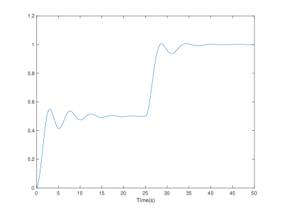
(a) Control

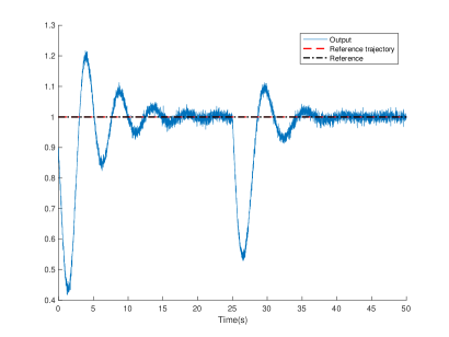
(b) Output

Figure 1: Integral feedback, constant reference trajectory, control efficiency loss

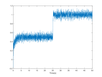
(a) Control

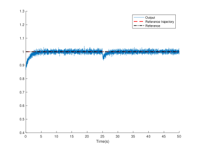
(b) Output

Figure 2: iP, constant reference trajectory, control efficiency loss

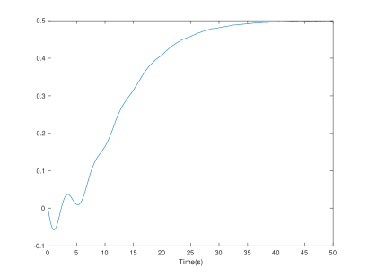
(a) Control

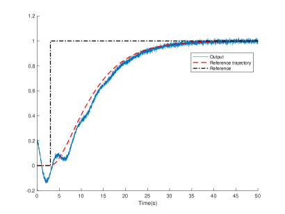
(b) Output

Figure 3: Integral feedback, slow connection

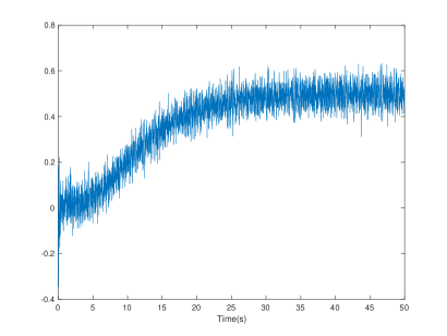
(a) Control

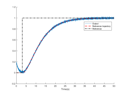
(b) Output

Figure 4: iP, slow connection

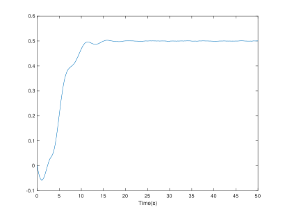
(a) Control

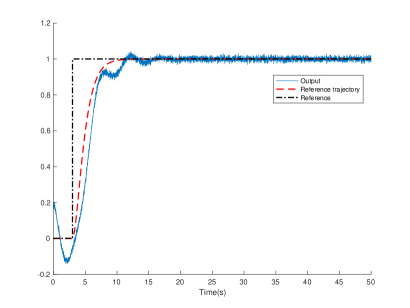
(b) Output

Figure 5: Integral feedback, fast connection

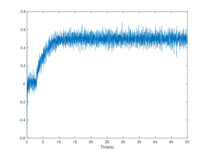
(a) Control

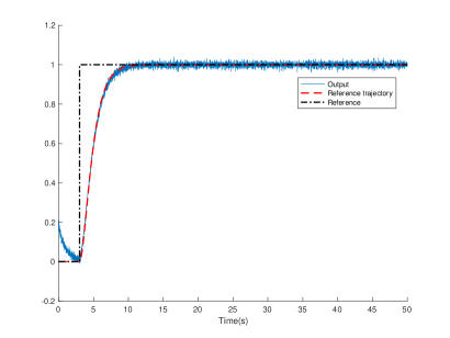
(b) Output

Figure 6: iP, fast connection

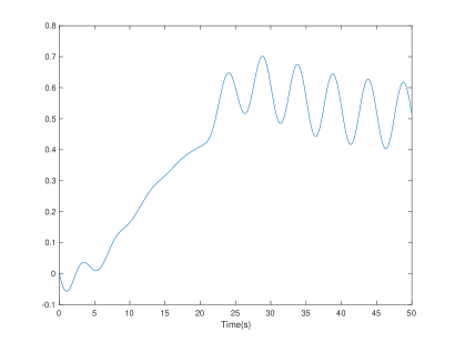
(a) Control

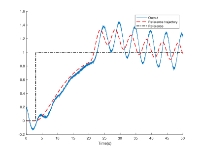
(b) Output

Figure 7: Integral connection, complex reference trajectory

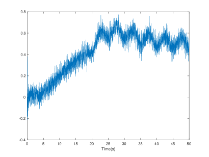
(a) Control

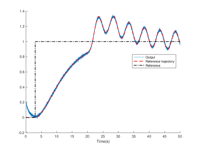
(b) Output

Figure 8: iP, complex reference trajectory

4.2 Nonlinear case

Consider

$$\dot{y}+y=u^{3}+P_{\text{pert}}$$

where $P_{\text{pert}}$ is a perturbation. Introduce three scenarios:

• Setpoint without any perturbation, i.e., $P_{\text{pert}}=0$: see Figures 9 and 10.

• Setpoint with a sine wave perturbation which starts at $t=25$s, i.e., $P_{\text{pert}}(t)=0.2\sin(\frac{2\pi}{5}(t-25))$ if $t\geq 25$s, and $P_{\text{pert}}(t)=0$ if $t\leq 25$s: see Figures 11 and 12.

• Non-constant reference trajectory without any perturbation, i.e., $P_{\text{pert}}=0$: see Figures 13 and 14.

A clear-cut superiority of the iP with respect to the integral feedback is indisputable. The behavior of dynamic compensation (resp. exact adaptation) is always (resp. never) satisfactory.

Remark 4.1

Do not believe that integral feedbacks are never adequate if nonlinearities occur. See

• an example related to ramp metering in Abouaïssa et al. [2017b],

• theoretical investigations in Sontag [2010].

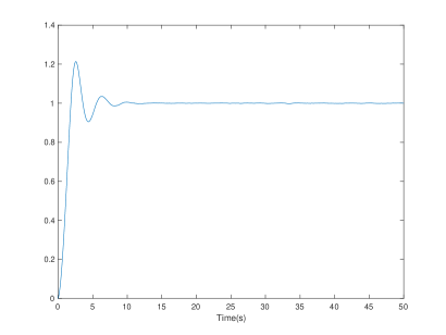
(a) Control

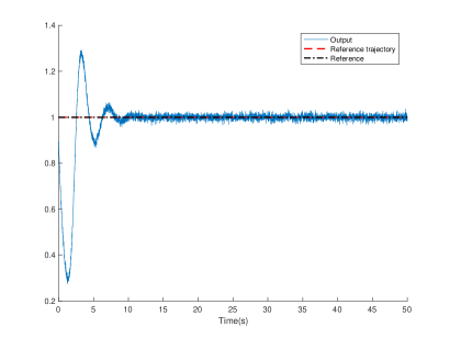
(b) Output

Figure 9: Integral feedback, constant reference trajectory, without any perturbation

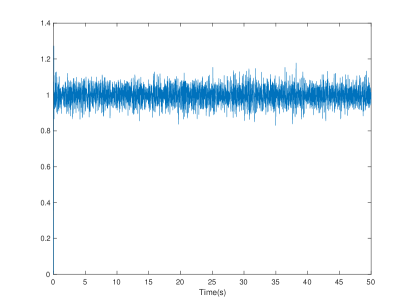
(a) Control

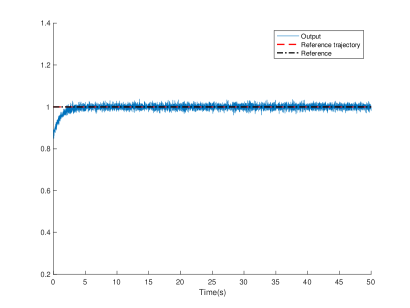
(b) Output

Figure 10: iP, constant reference trajectory, without any perturbation

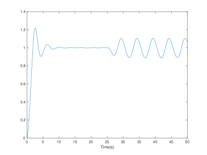
(a) Control

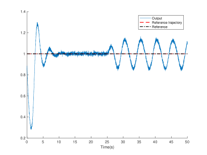
(b) Output

Figure 11: Integral feedback, constant reference trajectory, with perturbation

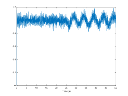
(a) Control

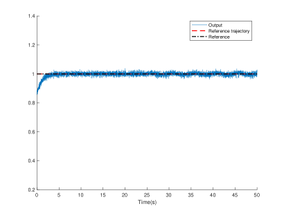
(b) Output

Figure 12: iP, constant reference trajectory, with perturbation

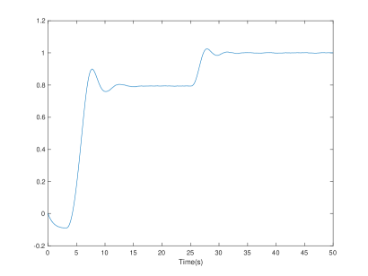
(a) Control

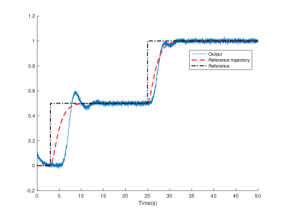
(b) Output

Figure 13: Integral feedback, non-constant reference trajectory, without any perturbation

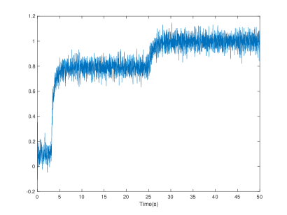
(a) Control

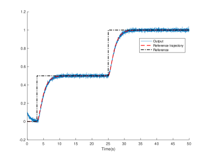
(b) Output

Figure 14: iP, non-constant reference trajectory, without any perturbation

5 Conclusion

In order to be fully convincing, this preliminary annoucement on homeostasis extensions needs of course to exhibit true biological examples. In our context noise corruption is also a hot topic (see, e.g., Briat et al. [2016], Sun et al. [2010]). The estimation and identification techniques sketched in Section 2.1 might lead to a better understanding (see also Fliess [2006, 2008]).

References

- Abouaïssa et al. [2017a] Abouaïssa H., Alhaj Hasan O., Join C., Fliess M., Defer D. (2017a). Energy saving for building heating via a simple and efficient model-free control design: First steps with computer simulations. 21st Int. Conf. Syst. Theor. Contr. Comput., Sinaia. https://hal.archives-ouvertes.fr/hal-01568899/en/
- Abouaïssa et al. [2017b] Abouaïssa H., Fliess M., Join C. (2017b). On ramp metering: Towards a better understanding of ALINEA via model-free control. Int. J. Contr., 90, 1018-1026.
- Alon [2006] Alon U. (2006). An Introduction to Systems Biology: Design Principles of Biological Circuits. Chapman and Hall.
- Alon et al. [1999] Alon U., Surette M.G., Barkai N., Leibler S. (1999). Robustness in bacterial chemotaxis. Nature, 397, 168-171.
-
d’Andréa-Novel et al. [2010]
d’Andréa-Novel B., Fliess M., Join C., Mounier H., Steux B. (2010). A mathematical explanation via “intelligent” PID controllers of the strange ubiquity of PIDs.
18th Medit. Conf. Contr. Automat., Marrakech.
https://hal.archives-ouvertes.fr/inria-00480293/en/ - Åström et al. [2008] Åström K.J., Murray R.M. (2008). Feedback Systems: An Introduction for Scientists and Engineers. Princeton University Press.
- Bara et al. [2016] Bara O., Fliess M., Join C., Day J., Djouadi S.M. (2016). Model-free immune therapy: A control approach to acute inflammation. Europ. Contr. Conf., Aalborg. https://hal.archives-ouvertes.fr/hal-01341060/en/
- Bourbaki [1976] Bourbaki N. (1976). Fonctions d’une variable réelle. Hermann. English translation (2004): Functions of a Real Variable. Springer.
- Briat et al. [2016] Briat C., Gupta A., Khammash M. (2016). Antithetic integral feedback ensures robust perfect adaptation in noisy biomolecular networks. Cell Syst., 2, 15-26.
- Cowan et al. [2014] Cowan N.J., Ankarali M.M., Dyhr J.P., Madhav M.S., Roth E., Sefati S., Sponberg S., Stamper S.A., Fortune E.S., Daniel T.L. (2014). Feedback control as a framework for understanding tradeoffs in biology. Integr. Compar. Biol., 54, 223-237.
- Cosentino et al. [2011] Cosentino C., Bates D. (2011). An Introduction to Feedback Control in Systems Biology. CRC Press.
- Del Vecchio et al. [2016] Del Vecchio D., Dy A.J., Qian Y. (2016). Control theory meets synthetic biology. J. Roy. Soc. Interface, 13: 20160380. http://dx.doi.org/10.1098/rsif.1916.0380
- Del Vecchio et al. [2015] Del Vecchio D., Murray R.M. (2015). Biomolecular Feedback Systems. Princeton University Press.
- Erdélyi [1962] Erdélyi A. (1962). Operational Calculus and Generalized Functions. Holt Rinehart Winston.
- Fliess [2006] Fliess M. (2006). Analyse non standard du bruit. C. R. Math., 342, 797-802.
-
Fliess [2008]
Fliess M. (2008). Critique du rapport signal à bruit en communications numériques. Revue Afric. Recher. Informat. Math. Appli., 9, 419-429.
https://hal.archives-ouvertes.fr/inria-00311719/en/ - Fliess et al. [2013] Fliess M., Join C. (2013). Model-free control. Int. J. Contr., 86, 2228-2252.
- Fliess et al. [2003] Fliess M., Sira-Ramírez H. (2003). An algebraic framework for linear identification. ESAIM Contr. Optimiz. Calc. Variat., 9, 151-168.
- Fliess et al. [2008] Fliess M., Sira-Ramírez H. (2008). Closed-loop parametric identification for continuous-time linear systems via new algebraic techniques. H. Garnier & L. Wang (Eds): Identification of Continuous-time Models from Sampled Data, Springer, pp. 362-391.
- Join et al. [2017a] Join C., Bernier J., Mottelet S., Fliess M., Rechdaoui-Guérin S., Azimi S., Rocher V. (2017a). A simple and efficient feedback control strategy for wastewater denitrification. 20th World Congr. Int. Feder. Automat. Contr., Toulouse. https://hal.archives-ouvertes.fr/hal-01488199/en/
-
Join et al. [2013]
Join C., Chaxel F., Fliess M. (2013). “Intelligent” controllers on cheap and small programmable devices. 2nd Int. Conf. Contr. Fault-Tolerant Syst., Nice.
https://hal.archives-ouvertes.fr/hal-00845795/en/ -
Join et al. [2017b]
Join C., Delaleau E., Fliess M., Moog C.H. (2017b). Un résultat intrigant en commande sans modèle. ISTE OpenScience Automat., 1, 9 p.
https://hal.archives-ouvertes.fr/hal-01628322/en/ - Karin et al. [2017a] Karin O., Alon U. (2017a). Biphasic response as a mechanism against mutant takeover in tissue homeostasis circuits. Molec. Syst. Biol., 13, 933.
- Karin et al. [2017b] Karin O., Alon U., Sontag E. (2017b). A note on dynamical compensation and its relation to parameter identifiability. bioRxiv doi: https://doi.org/10.1101/123489
- Karin et al. [2016] Karin O., Swisa A., Glaser B., Dor Y., Alon U. (2016). Dynamical compensation in physiological circuits. Mol. Syst. Biol., 12: 886. DOI 10.15252/msb.19167216
- Klipp et al. [2016] Klipp E., Liebermeister W., Wierling C., Kowald A. (2016). Systems Biology (nd ed.). Wiley-VCH.
- Kremling [2012] Kremling A. (2012). Kompendium Systembiologie – Mathematische Modellierung und Modellanalyse. Vieweg + Teubner. English translation (2014): Systems Biology. CRC Press.
- Küpfmüller et al. [2017] Küpfmüller K., Mathis W., Reibiger, W. (2017). Theoretische Elektrotechnik – Eine Einführung (20. Auflage).777The first edition was published in 1932. Karl Küpfmüller was its sole author. He died in 1977. Springer.
- Lafont et al. [2015] Lafont F., Balmat J.-F., Pessel N., Fliess M. (2015). A model-free control strategy for an experimental greenhouse with an application to fault accommodation. Comput. Electron. Agricult., 110, 139–149.
- Menhour et al. [2017] Menhour L., d’Andréa-Novel B., Fliess M., Gruyer D., Mounier H (2017). An efficient model-free setting for longitudinal and lateral vehicle control. Validation through the interconnected pro-SiVIC/RTMaps prototyping platform. IEEE Trans. Intel. Transport. Syst., 2017. DOI: 10.1109/TITS.1917.2699283
- Miao et al. [2011] Miao H., Xia X., Perelson A.S., Wu H. (2011). On identifiability of nonlinear ODE models and applications in viral dynamics. SIAM Rev., 53, 3-39.
- MohammadRidha et al. [2018] MohammadRidha T., Aït-Ahmed M., Chailloux L., Krempf M., Guilhem I., Poirier J.-Y., Moog C.H. (2018). Model free iPID control for glycemia regulation of type-1 diabetes. IEEE Trans. Biomed. Engin., 65, 199-206.
- O’Dwyer [2009] O’Dwyer A. (2009). Handbook of PI and PID Controller Tuning Rules (3rd ed.). Imperial College Press.
- Sira-Ramírez et al. [2014] Sira-Ramírez H., García-Rodríguez C., Cortès-Romero J., Luviano-Juárez A. (2013). Algebraic Identification and Estimation Methods in Feedback Control Systems. Wiley.
- Somvanshi et al. [2015] Somvanshi P.R., Patel A.K, Bhartiya S., Venkatesh K.V. (2015). Implementation of integral feedback control in biological systems. Wiley Interdisc. Rev.: Syst. Biol. Med., 7, 301-316.
- Sontag [2010] Sontag E.D. (2010). Remarks on feedforward circuits, adaptation, and pulse memory. IET Syst. Biol., 4, 39-51.
- Sontag [2017] Sontag E.D. (2017). Dynamic compensation, parameter identifiability, and equivariances. PLoS Comput. Biol., 13: e1005447. doi: 10.1371/journal.pcbi.1005447
- Sun et al. [2010] Sun L., Becskei A. (2010). The cost of feedback control. Nature, 467, 163-164.
- Stelling et al. [2004] Stelling J., Sauer U., Szallasi Z., Doyle F.J., Doyle J. (2004). Robustness of cellular functions. Cell, 118, 675-685.
- Tebbani et al. [2016] Tebbani S., Titica M., Join C., Fliess M., Dumur D. (2016). Model-based versus model-free control designs for improving microalgae growth in a closed photobioreactor: Some preliminary comparisons. 24th Medit. Conf. Contr. Automat., Athens. https://hal.archives-ouvertes.fr/hal-01312251/en/
-
Villaverde et al. [2017]
Villaverde A.F., Banga J.R. (2017). Dynamical compensation and structural identifiability of biological models: Analysis, implications, and reconciliation. PLoS Comput. Biol., 13, e1005878.
https//doi.org/10.1371/journal.pcbi.1005878 - Yi et al. [2000] Yi T.-M., Huang Y., Simon M.I., Doyle J. (2000). Robust perfect adaptation in bacterial chemotaxis through integral feedback control. Proc. Nat. Acad. Sci., 97, 4649-4653.
- Zeron [2008] Zeron E.S. (2008). Positive and negative feedback in engineering and biology. Math. Model. Nat. Phenom., 3, 67-84.