Physics with Reactor Neutrinos

Abstract

Neutrinos produced by nuclear reactors have played a major role in advancing our knowledge of the properties of neutrinos. The first direct detection of the neutrino, confirming its existence, was performed using reactor neutrinos. More recent experiments utilizing reactor neutrinos have also found clear evidence for neutrino oscillation, providing unique input for the determination of neutrino mass and mixing. Ongoing and future reactor neutrino experiments will explore other important issues, including the neutrino mass hierarchy and the search for sterile neutrinos and other new physics beyond the standard model. In this article, we review the recent progress in physics using reactor neutrinos and the opportunities they offer for future discoveries.

Keywords: reactor neutrinos, neutrino oscillation, lepton flavor, neutrino mixing angles, neutrino masses

1 Introduction

Neutrinos are among the most fascinating and enigmatic particles in nature. The standard model in particle physics includes neutrinos as one of the fundamental point-like building blocks. Processes involving the production and interaction of neutrinos provided crucial inputs for formulating the electroweak theory, unifying the electromagnetic and weak interactions. Neutrinos also play a prominent role in cosmology. The abundant neutrinos produced soon after the big bang offer the potential to view the Universe at an epoch much earlier than that accessible from the cosmic microwave background. The direct detection of these ‘relic’ neutrinos from the big bang remains a major experimental challenge. For a long time, these neutrinos were also considered a prime candidate for dark matter. While this is no longer viable given the current upper limit on the neutrino mass, neutrinos nevertheless constitute a non-negligible fraction of the invisible mass in the Universe.

Neutrinos also play an important role in astrophysics. Detection of neutrinos emitted in a supernova explosion reveals not only the mechanisms of supernova evolution but also the properties and interactions of neutrinos in a super dense environment. Extensive efforts are also dedicated to the search for ultra-high-energy extra-galactic neutrinos. The charge-neutral neutrinos can potentially be traced back to locate the sources of ultra-high-energy cosmic rays.

Neutrino beams from accelerators have also been employed to probe the quark structures of nucleons and nuclei via deep inelastic scattering (DIS). Experiments using neutrino beams, together with those with charged lepton beams, have provided crucial tests to validate QCD as the theory for strong interactions.

Observations of neutrino mixings and the existence of three non-degenerate neutrino mass eigenstates have provided the only unambiguous evidence so far for physics beyond the standard model. The origin of such tiny neutrino mass remains a mystery and could reveal new mechanisms other than the Higgs mechanism for mass generation. Neutrinos may also be a portal for approaching the dark sector. Mixing between the standard model neutrinos with ‘sterile’ neutrinos in the dark sector could lead to observable effects.

The purpose of this article is to review recent progress in neutrino physics obtained from experiments performed near nuclear reactors. As a prolific and steady source of electron antineutrinos, nuclear reactors have been a crucial tool for understanding some fundamental properties of neutrinos. In fact, the first detection of neutrinos was from a reactor neutrino experiment . To illustrate the important roles of reactors for neutrino physics, we first briefly review the history of the discovery of neutrino.

In his famous letter to “radioactive ladies and gentlemen”, Pauli postulated [1] in 1930 the existence of a new charge-neutral weakly interacting particle emitted undetected in nuclear beta decay. This spin-1/2 particle would not only resolve the outstanding puzzle of energy non-conservation, but also explain the apparent violation of angular momentum conservation in nuclear beta decay. Soon after Pauli’s neutrino postulate, Fermi formulated [2, 3] in 1933 his celebrated theory of nuclear beta decay, taking into account Pauli’s neutrino, and successfully explained the experimental data. While Fermi’s theory provided convincing evidence for the existence of the neutrino, a direct detection of the neutrino had to wait for many years. The prospect for directly detecting the neutrino was considered by Bethe and Peierls [4], who suggested the so-called ‘inverse beta decay’ (IBD), $\bar{\nu}_{e}+p\to e^{+}+n$, as a possible reaction to detect the neutrino. However, they estimated a tiny IBD cross section ($\sim$10^-42 cm²), prompting them to conclude that “…there is no practically possible way of observing the neutrino.” Responding to this conclusion, Pauli commented that “I have done something very bad by proposing a particle that cannot be detected; it is something no theorist should ever do [5].”

The advent of nuclear reactors as a steady and intense source of electron antineutrinos ($\bar{\nu}_{e}$) and the development of large volume liquid scintillator detectors opened the door for Fred Reines and Clyde Cowan to perform the pioneering experiments at the Hanford [6] and Savanah River [7, 8] nuclear reactors to detect neutrinos directly via the IBD reaction suggested by Bethe and Peierls. A crucial feature of the IBD reaction is the time correlation between the prompt signal from the ionization and annihilation of $e^{+}$ and the delayed signal from the $\gamma$ rays produced in the neutron capture. This distinctive pattern in time correlation allows a powerful rejection of many experimental backgrounds [9].

Upon the definitive observation of neutrinos via the IBD reaction, Reines and Cowan sent a telegram on June 14, 1956, to Pauli informing him that “..we have definitely detected neutrinos from fission fragments by observing inverse beta decay”. Pauli replied that “Everything comes to him who knows how to wait” [5]. Indeed, it took 26 years for Pauli’s neutrino to be detected experimentally. It would take another 30 years before Reines received the Nobel Prize for his pioneering experiment.

In addition to discovering the neutrino via the IBD reaction, Reines, Cowan, and collaborators also reported several pioneering measurements using their large liquid scintillator detectors. They performed the first search for the neutrino magnetic moment via $\nu-e$ elastic scattering, setting an upper limit at $\sim$10^-7 Bohr magnetons initially [10], which was later improved to $\sim$10^-9 Bohr magnetons using a larger detector [11]. A search for proton stability was also carried out, resulting in a lifetime of free protons (bound nucleons) greater than $10^{21}$ ($10^{22}$) yr. By inserting a sample of Nd₂O₃ enriched in ¹⁵⁰Nd inside the liquid scintillator, they searched for neutrinoless double beta decay from ¹⁵⁰Nd and set a lower limit on the half-life at $2.2\times 10^{18}$ yr [12]. It is truly remarkable that searches for the neutrino magnetic moment, proton decay, and neutrinoless double beta decay are still among the most important topics being actively pursued, using techniques similar to those developed by Reines and Cowan. The favored reaction to detect reactor electron antineutrinos to date remains IBD, and large liquid scintillators are currently utilized or being constructed for a variety of fundamental experiments.

As recognized by Pauli when he first put forward his neutrino hypothesis, the neutrino must have a tiny mass, comparable or lighter than that of the electron [1]. Later, Fermi’s theory for beta decay was found to be in excellent agreement with experimental data when a massless neutrino was assumed. Indeed, Fermi was in favor of a massless neutrino as a simple and elegant scenario, putting the neutrino in the same class of particles as the photon and the graviton [13]. A finite neutrino mass could be revealed from a precise measurement of the endpoint energy of nuclear beta decay, notably tritium beta decay. While the precision of tritium beta decay experiments continued to improve, yet no definitive evidence for a finite neutrino mass was found [14]. As one of the most abundant particles in the Universe, the exact value of the neutrino mass has implications not only on particle physics, but also on cosmology and astrophysics. The quest for determining the neutrino mass remains an active and exciting endeavor today.

Inspired by the mixing phenomenon observed in the neutral kaon system, Pontecorvo suggested the possibility of neutrino-antineutrino mixing and oscillation [15, 16]. After the muon neutrino was discovered, this idea was extended to the possible mixing and oscillation between neutrinos of different flavors (i.e., mixing between the electron neutrino and muon neutrino) [17, 18, 19]. Neutrino oscillation is a quantum mechanical phenomenon when neutrinos are produced in a state that is a superposition of eigenstates of different mass. As such, this oscillation is possible only when at least one neutrino mass eigenstate possesses a non-zero mass. The pattern of the oscillation, if found, will directly reveal the amount of mixing (in terms of mixing angle), as well as mass-squared difference (i.e., $\Delta m^{2}_{21}\equiv m_{2}^{2}-m_{1}^{2}$). Thus, neutrino oscillation provided an exciting new venue to search for a tiny neutrino mass, beyond the reach of any foreseeable nuclear beta decay experiments.

Searches for the phenomenon of neutrino oscillation were pursued in earnest using a variety of man-made and natural sources of neutrinos. In the early 1980s, two reactor neutrino experiments reported possible evidence for neutrino oscillation. The experiment performed by Reines and collaborators [20] at the Savannah River reactor found an intriguing difference between the detected number of electron antineutrinos and the sum of electron and other types of antineutrinos using a deuteron (heavy water) target. The distinctions among different types of neutrino flavors were made possible through the observation of neutral-current as well as charged-current disintegration of the deuteron, a method adopted later by the SNO solar neutrino experiment. The larger number of neutrinos observed for the neutral-current events than that for the charged-current ones suggested that some electron neutrinos had oscillated into other types of neutrinos as they traveled from the reactor to the detector.

The other tantalizing evidence [21] for neutrino oscillation was obtained by detecting IBD events at two distances, 13.6 and 18.3 meters, from the core of the Bugey reactor in France. From a comparison of detected IBD events at the two distances, for which the uncertainties of the flux and energy spectrum of the neutrino source largely canceled, a smaller than expected number of detected IBD events at the larger distance was interpreted as evidence for oscillation.

Although later reactor experiments [22, 23, 24, 25] performed in the 1980s and 1990s did not confirm the earlier results on neutrino oscillation, interest continued to grow in finding neutrino oscillation with larger and better detectors using intense reactor neutrino sources. The first observation of reactor neutrino oscillation was reported in 2002 by the KamLAND experiment [26]. Amusingly, while earlier experiments were located at relatively short distances from the reactors in order to have reasonable event rates, KamLAND was situated at an average distance of $\sim$180 km from the neutrino sources. At such a large distance, corresponding to a long oscillation period, the relevant neutrino mass scale is tiny, of the order of $\Delta m^{2}\sim$10^-4 eV². This long distance allows one to probe the large mixing angle (LMA) solution, one of the few possible explanations to the solar neutrino problem (see Sec. 3.2 for more details). The KamLAND result, together with the analysis [27] of experiments reporting the observation of solar neutrino oscillation, allowed an accurate determination of the mixing angle ($\theta_{12}$) governing these oscillations. The KamLAND result remains the best measurement of $\Delta m^{2}_{21}$.

Starting from the late 1980s, evidence for neutrino oscillation was reported by the large underground detectors including Kamiokande [28, 29] and Super-Kamiokande [30], which detected energetic electron and muon neutrinos ($\sim$GeV) originating from the decay of mesons produced in the interaction of cosmic rays in Earth’s atmosphere. These results suggested the possibility of observing oscillation for reactor neutrinos at a distance of $\sim$1 km. Two reactor neutrino experiments, CHOOZ [31, 32] and Palo Verde [33], were constructed specifically to look for such oscillations. However, no evidence for oscillation was found within the sensitivities of both experiments. The CHOOZ experiment set an upper limit at 0.12 (90% C.L.) for $\sin^{2}2\theta_{13}$ [32]. Together with other oscillation experiments, in particular Super-Kamiokande, these results indicated a very small value, possibly zero, for the mixing angle $\theta_{13}$, which dictates the amplitude of the reactor neutrino oscillation at this distance scale.

As one of the fundamental parameters describing the properties of neutrinos, $\theta_{13}$ is also highly relevant for the phenomenon of CP-violation in the neutrino sector. The importance of the as yet unknown mixing angle $\theta_{13}$ led to a worldwide effort to measure it in high-precision experiments. Around 2006, three reactor neutrino experiments, Daya Bay, Double Chooz, and RENO, were proposed to probe $\theta_{13}$. All three experiments have already collected unprecedentedly large numbers of neutrino events. Evidence for non-zero values of $\theta_{13}$, deduced from the observation of neutrino oscillation at a 1$\sim$2 kilometer distance, has emerged from all three experiments [34, 35, 36]. Despite being the smallest among the three neutrino mixing angles in the standard three-neutrino paradigm, $\theta_{13}$ is nevertheless the most precisely determined to date.

Discovery of a non-zero $\theta_{13}$ mixing angle is an important milestone in neutrino physics. The precise measurement of $\theta_{13}$ not only provides a crucial input for model-building in neutrino physics, but also inspires new reactor neutrino experiments to explore other important issues in neutrino physics, such as determining the neutrino mass hierarchy [37] and searching for sterile neutrinos [38]. It is remarkable that all ongoing and planned reactor neutrino experiments adopt essentially the same techniques pioneered by Reines and Cowan and their coworkers over 60 years ago.

The focus of this review is on the three ongoing reactor neutrino experiments, Daya Bay, Double Chooz, and RENO. These experiments share many common features, and we will in some cases discuss one of these experiments as a specific example. Previous review articles on reactor neutrino physics are also available [39, 40, 41, 42]. The organization of this review article is as follows. Section 2 describes the salient characteristics of the antineutrinos produced in nuclear reactors as well as the experimental techniques for detecting them. The subject of reactor neutrino oscillation is discussed in Sec. 3. The discussion regarding the reactor antineutrino anomaly and the search for a light sterile neutrino is presented in Sec. 4. Some additional physics topics accessible in reactor neutrino experiments are described in Sec. 5, followed by conclusions in Sec. 6.

2 Production and Detection of Reactor Neutrinos

To date, five main natural and man-made neutrino sources have played crucial roles in advancing our knowledge of neutrino properties. They are: i) reactor electron antineutrinos ($\bar{\nu}_{e}$) produced through fission processes; ii) accelerator neutrinos ($\nu_{\mu}$, $\nu_{e}$, $\bar{\nu}_{\mu}$, and $\bar{\nu}_{e}$) resulting from decays of mesons created by proton beams bombarding a production target; iii) solar neutrinos ($\nu_{e}$) generated via fusion processes in the sun; iv) supernova neutrinos (all flavors) produced during supernova explosions; and v) atmospheric neutrinos ($\nu_{\mu}$, $\nu_{e}$, $\bar{\nu}_{\mu}$, and $\bar{\nu}_{e}$) created through decays of mesons produced by the interaction of high-energy cosmic rays with Earth’s atmosphere. Beside these, geoneutrinos produced from radionuclide inside the Earth and extra-galactic ultra-high energy neutrinos have also been detected.

Compared to atmospheric and accelerator neutrinos, reactor neutrinos have the advantage of being a source of pure flavor ($\bar{\nu}_{e}$ with energy up to $\sim$10 MeV). In addition, the primary reactor neutrino detection channel, IBD, is well understood theoretically and allows an accurate measurement of the neutrino energy, unlike high-energy neutrino–nucleus interactions. Compared to rates for solar and supernova neutrinos, the event detection rate of reactor neutrinos can be much larger, as detectors can be placed at distances close to the source. In this Section, we review the production and detection of reactor neutrinos.

2.1 Production of Reactor Neutrinos

Energy is generated in a reactor core through neutron-induced nuclear fission. This process is maintained by neutrons emitted in fission. For example, the average number of emitted neutrons is about 2.44 per ²³⁵U fission [44], among which, on average, only one neutron will induce a new fission reaction for a controlled reactor operation.

While the fission of ²³⁵U is the dominating process in a research reactor using highly enriched uranium (HEU) fuel ($>$20$\%$ ²³⁵U concentration), more fissile isotopes are involved in a commercial power reactor using low enriched uranium (LEU) fuel (3–5% ²³⁵U concentration). Inside the core of a commercial power reactor, a portion of the neutrons are captured by ²³⁸U because of its much higher concentration, producing new fissile isotopes: ²³⁹Pu and ²⁴¹Pu. Fissions of ²³⁵U, ²³⁹Pu, and ²⁴¹Pu are induced by thermal neutrons ($\sim$0.025-eV kinetic energy). In contrast, fission of ²³⁸U can be induced only by fast neutrons ($\sim$1-MeV kinetic energy). The average number of emitted neutrons are 2.88 [44], 2.95 [44], and 2.82 [45] per ²³⁹Pu, ²⁴¹Pu, and ²³⁸U fission, respectively.

The reactor neutrinos are mainly produced through the beta-decays of the neutron-rich fission daughters of these four isotopes, in which a bound neutron is converted into a proton while producing an electron and an electron antineutrino. Besides the fission processes, another important source of $\bar{\nu}_{e}$ originates from neutron capture on ²³⁸U: ²³⁸U$(n,\gamma)^{239}$U. The beta decay of ²³⁹U (Q-value of 1.26 MeV and half-life of 23.5 mins) and the subsequent beta decay of ²³⁹Np (Q-value of 0.72 MeV and half-life of 2.3 days) produce a sizable amount of $\bar{\nu}_{e}$ at low energies. An average of $\sim$6 $\bar{\nu}_{e}$ were produced per fission, leading to $\sim$2$\times 10^{20}$ $\bar{\nu}_{e}$ emitted every second isotropically for each GW of thermal power.

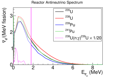
Figure 1: The $\bar{\nu}_{e}$ energy spectra for ²³⁵U, ²³⁸U, ²³⁹Pu, and ²⁴¹Pu fissions. Above the inverse beta decay (IBD) threshold (marked by the vertical line), spectra from Ref. [46, 47] are shown. Below the IBD threshold, spectra are plotted based on Table II of Ref. [48]. Fine structures at the end points of various decay branches cannot be seen, given the coarse binning. In addition, we show the antineutrino spectrum produced by neutron capture on ²³⁸U (taken from Ref. [49]), which is normalized properly relative to the ²³⁸U fission and scaled down by a factor of 20 for the display.

The expected $\bar{\nu}_{e}$ energy spectra are shown in Fig. 1. The magnitude of $\bar{\nu}_{e}$ spectra for ²³⁸U (²⁴¹Pu) are larger than that of ²³⁵U (²³⁹Pu), because more neutron-rich fissile isotopes lead to more beta-unstable neutron-rich fission daughters. In addition, the $\bar{\nu}_{e}$ energy spectrum is considerably harder for the fast-neutron-induced ²³⁸U fission chain than the other three thermal-neutron induced fission chains.

For commercial power reactors burning LEU, typical average values of fission fractions during operation are around 58%, 29%, 8%, and 5% for ²³⁵U, ²³⁹Pu, ²³⁸U, and ²⁴¹Pu, respectively. Roughly 30% of the antineutrinos (two out of the average six antineutrinos produced per fission) have energies above 1.8 MeV, which is the energy threshold of the IBD process. In particular, the low-energy $\bar{\nu}_{e}$ produced by neutron capture on ²³⁸U is irrelevant for detection through IBD. In the following, we describe two principal approaches for calculating the antineutrino flux and energy spectrum. More details can be found in a recent review [50].

In the first approach, the flux and spectrum can be predicted by the cumulative fission yields $Y_{n}(t)$ at time $t$ for fission product of nucleus $n$ having a mass number $A$ and an atomic number $Z$, branching ratios $b_{n,i}$ of $\beta$-decay branch $i$ with endpoints $E_{0}^{n,i}$, and the energy spectrum of each of $\beta$ decays $P(E_{\bar{\nu}},E_{0}^{n,i})$:

$$\frac{dN}{dE_{\bar{\nu}}}=\sum_{n}Y_{n}(t)\cdot\left(\sum_{i}b_{n,i}\cdot P(E_{\bar{\nu}},E_{0}^{n,i})\right).$$ (1)

This method was recently used in Ref. [47] and included about 10k beta decay branches, following the early work in Refs. [51, 52, 53, 54, 55]. Despite being straightforward, several challenges in this method lead to large uncertainties in predicting the flux and spectrum. First, the fission yields, $\beta$-decay branching ratios, and the endpoint energies are sometimes not well known, especially for short-lived fragments having large beta-decay Q values. Second, the precise calculation of the individual spectrum shape $P(E_{\bar{\nu}},E_{0}^{n,i})$ requires a good model of the Coulomb distortions (including radiative corrections, the nuclear finite-size effects, and weak magnetism) in the case of an allowed decay type having zero orbital angular momentum transfer. Finally, many of the decay channels are of the forbidden types having non-zero orbital angular momentum transfer. For example, about 25% of decays are the first forbidden type involving parity change, in which the individual spectrum shape $P(E_{\bar{\nu}},E_{0}^{n,i})$ is poorly known. Generally, a 10–20% relative uncertainty on the antineutrino spectra is obtained using this method.

Another method uses experimentally measured electron spectra associated with the fission of the four isotopes to deduce the antineutrino spectra. The electron energy spectra for the thermal neutron fission of ²³⁵U, ²³⁹Pu, and ²⁴¹Pu have been measured at Institut Laue–Langevin (ILL) [56, 57, 58]. The electron spectrum associated with the fast neutron fission of ²³⁸U has been measured in Münich [59]. Since the electron and the $\bar{\nu}_{e}$ share the total energy of each $\beta$-decay branch, ignoring the negligible nuclear recoil energy, the $\bar{\nu}_{e}$ spectrum can be deduced from the measured electron spectrum.

The procedure involved fitting the electron spectrum to a set of $\sim$30 virtual branches having equally spaced endpoint energies, assuming all decays are of the allowed type. For each virtual branch, the charge of parent nucleus $Z$ is taken from a fit to the average $Z$ of real branches as a function of the endpoint energy. The conversion to the $\bar{\nu}_{e}$ spectrum is then performed in each of these virtual branches using their fitted branching ratios. This conversion method was used in Refs. [47, 56, 57, 58, 60].

In addition to the experimental uncertainties associated with the electron spectrum, corrections to the individual $\beta$-decay branch resulting from radiative correction, weak magnetism, and finite nuclear size also introduce uncertainties. With these contributions, the model uncertainty in the flux is estimated to be $\sim$2% [46, 47]. However, the uncertainties resulting from spectrum shape and magnitude of the numerous first forbidden $\beta$ decays can be substantial [61]. When the first forbidden decays are included, the estimated uncertainty increases to $\sim$5% [61]. Besides these model uncertainties, the total experimental uncertainty of the $\bar{\nu}_{e}$ spectrum further includes the contribution from the thermal power of the reactor, its time-dependent fuel composition (i.e., fission fractions), and fission energies associated with ²³⁵U, ²³⁸U, ²³⁹Pu, and ²⁴¹Pu.

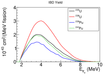
Figure 2: Inverse beta decay yields from the convolution of the IBD cross section and the antineutrino spectra for ²³⁵U, ²³⁸U, ²³⁹Pu, and ²⁴¹Pu.

2.2 Detection of Reactor Neutrinos

Table 1: Summary of various $\bar{\nu}_{e}$ detection methods. CC (NC) stands for the charged-current (neutral-current) interaction. The cross section is integrated over the entire reactor neutrino energy spectrum. $N$ stands for the number of neutrons in the target nucleus. For these estimations, fission fractions are assumed to be 58%, 29%, 8%, and 5% for ²³⁵U, ²³⁹Pu, ²³⁸U, and ²⁴¹Pu, respectively.

Channel	Interaction	Cross Section	Threshold
	Type	($10^{-44}$ cm2/fission)	(MeV)
$\bar{\nu}_{e}+p\rightarrow e^{+}+n$	CC	$\sim$63	1.8
$\bar{\nu}_{e}+d\rightarrow n+n+e^{+}$	CC	$\sim$1.1	4.0
$\bar{\nu}_{e}+d\rightarrow n+p+\bar{\nu}_{e}$	NC	$\sim$3.1	2.2
$\bar{\nu}_{e}+e^{-}\rightarrow\bar{\nu}_{e}+e^{-}$	CC/NC	$\sim$0.4	0
$\bar{\nu}_{e}+A\rightarrow\bar{\nu}_{e}+A$	NC	$\sim$9.2$\times N^{2}$	0

In addition to the aforementioned IBD process, several methods can potentially be used to detect reactor neutrinos. The first method is the charged-current (CC) ($\bar{\nu}_{e}+d\rightarrow n+n+e^{+}$) and neutral-current (NC) deuteron break-up ($\bar{\nu}_{e}+d\rightarrow n+p+\bar{\nu}_{e}$) using heavy water as a target. These processes were used to compare the NC and CC cross sections [20, 62]. Similar processes involving $\nu_{e}$ were also used in the SNO experiment in detecting the flavor transformation of solar neutrinos [63].

The second method is the antineutrino-electron elastic scattering, $\bar{\nu}_{e}+e^{-}\rightarrow\bar{\nu}_{e}+e^{-}$, which combines the amplitudes of the charged-current (exchange of $W$ boson) and the neutral-current (exchange of $Z$ boson). The signature of this process would be a single electron in the final state. This process has been used to measure the weak mixing angle $\theta_{W}$ and to constrain anomalous neutrino electromagnetic properties [49, 64, 65, 66, 67]. Neutrino-electron scattering is also one of the primary approaches to detect solar neutrinos [63, 68, 69].

The third method is the coherent antineutrino-nucleus interaction, in which the signature is a tiny energy deposition by the recoil nuclei. Although coherent elastic neutrino-nucleus scattering was observed recently for the first time [70] using neutrinos produced in the decay of stopped pions, the observation for this process for less-energetic reactor neutrinos has not been achieved. Table 1 summarizes some essential information for these detection channels.

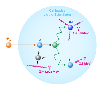
Figure 3: Principle of the IBD detection in a Gd-loaded liquid scintillator. The electron antineutrino interacts with a free proton. The ionization and annihilation of the final-state positron form the prompt signal. The capture of the recoil neutron on Gd (or H) gives the delayed signal.

Table 2: Various nuclei used in experiments to capture recoil neutrons from the IBD reaction. The detection channels and their cross sections [45] for thermal neutron capture are listed. ¹⁵⁷Gd has the highest thermal-neutron capture cross section of any stable nuclide.

Target nucleus	process	cross section (barn)
		for thermal neutron
H	$n+p\rightarrow d+\gamma~{}(2.2~{}{\rm MeV})$	$\sim$0.33
3He	$n+^{3}$He$\rightarrow p+^{3}$H$+0.764~{}{\rm MeV}$	$\sim$5300
6Li	$n+^{6}$Li$\rightarrow\alpha+^{3}$H$+4.6~{}{\rm MeV}$	$\sim$950
10B	$n+^{10}$B$\rightarrow\alpha+^{7}$Li$+6.2~{}{\rm MeV}$	$\sim$3,860
108Cd	$n+^{108}$Cd$\rightarrow^{109m}$Cd$\rightarrow^{109}$Cd$+\gamma~{}(0.059~{}{\rm MeV})$	$\sim$1000
Gd	$n+^{155}$Gd$\rightarrow^{156}$Gd$+\gamma s~{}(8.5~{}{\rm MeV})$	$\sim$61,000
	$n+^{157}$Gd$\rightarrow^{158}$Gd$+\gamma s~{}(7.9~{}{\rm MeV})$	$\sim$256,000

So far, the primary method to detect the reactor $\bar{\nu}_{e}$ is the IBD reaction: $\bar{\nu}_{e}+p\rightarrow e^{+}+n$. The energy threshold of this process is about 1.8 MeV, and the cross section is accurately known [71, 72]. At the zeroth order in 1/$M$, with $M$ being the nucleon mass, the cross section can be written as:

$$\sigma^{(0)}=\frac{G_{F}^{2}\cos^{2}\theta_{C}}{\pi}\left(1+\Delta^{R}_{inner}\right)\cdot\left(f^{2}+3g^{2}\right)\cdot E_{e}^{(0)}\cdot p_{e}^{(0)},$$ (2)

with $G_{F}$ being the Fermi coupling constant and $\theta_{C}$ being the Cabibbo angle. The vector and axial vector coupling constants are $f=1$ and $g=1.27$, respectively. $\Delta^{R}_{inner}$ represents the energy independent inner radiative corrections. $E_{e}$ and $p_{e}$ are the energy and momentum of the final-state positron having $E^{(0)}=E_{\nu}-(M_{n}-M_{p})$ after ignoring the recoil neutron kinetic energy. The IBD cross section can be linked to the neutron lifetime $\tau_{n}=880.2\pm 1.0$ s [14] as:

$$\sigma^{(0)} = \frac{2\pi^{2}/m_{e}^{2}}{f^{R}\tau_{n}}E^{(0)}_{e}\times p^{(0)}_{e}$$ (3)

$$\approx 9.52\times\left(\frac{E^{(0)}_{e}\cdot p^{(0)}_{e}}{{\rm MeV}^{2}}\right)\times 10^{-44}{\rm cm}^{2},$$

with $m_{e}$ being the mass of the electron and $f^{R}=1.7152$, representing the neutron decay phase space factor that includes the Coulomb, weak magnetism, recoil, and outer radiative corrections. The above formula represents the zeroth order in 1/$M$, and we should note that the corrections of the first order in $1/M$ are still important at reactor energies.

The various forms of extension to all orders in $1/M$, as well as the convenient numerical form of radiative corrections of order $\alpha/\pi$ can be found in Refs. [71, 72]. Figure 2 shows the IBD yield obtained from the convolution of the IBD cross section and the antineutrino energy spectra. While peak positions for the thermal neutron fission (²³⁵U, ²³⁹Pu, and ²⁴¹Pu) occur at an energy around 3.5 MeV, the peak position for fast-neutron fission (²³⁸U) is at a slightly higher energy, around 4 MeV. The IBD yield is also larger for the latter.

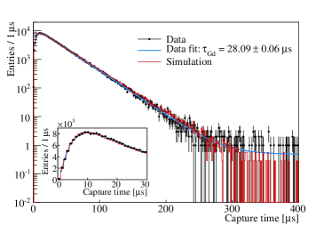
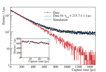
Figure 4: The time difference between prompt and delayed signals for a neutron captured on Gd (A) and hydrogen (B), taken from Ref. [73]. The data histograms contain backgrounds leading to non-exponential distributions visible at large capture times.

As shown in Fig. 3, an IBD event is indicated by a pair of coincident signals consisting of i) a prompt signal induced by positron ionization and annihilation inside the detector; and ii) a delayed signal produced by the neutron captured on a proton or a nucleus (such as Gd). Because of time correlation, IBD can be clearly distinguished from radioactive backgrounds, which usually contain no delayed signal.

The energy of the prompt signal is related to the neutrino energy via $E_{\bar{\nu}}\approx E_{prompt}+0.78~{}{\rm MeV}+T_{n}$, with $T_{n}$ being the kinetic energy of the recoil neutron. Since $T_{n}$, of the order of tens of keV, is much smaller than that of $\bar{\nu}_{e}$, the neutrino energy can be accurately determined by the prompt energy, which is a very attractive feature for measuring neutrino oscillation.

Table 2 summarizes various nuclei used in past experiments to capture recoil neutrons from the IBD reaction. For example, for a neutron captured on a proton, the delayed signal comes from a single 2.2-MeV $\gamma$ ray. In comparison, for a neutron captured on Gd, the delayed signal consists of a few $\gamma$ rays having the total energy of $\sim$8 MeV. For a pure liquid scintillator, the average time between the prompt and delayed signals is $\sim$210 $\mu$s. This is reduced to $\sim$30 $\mu$s for a 0.1% Gd-doped liquid scintillator because of the additional contribution of neutron capture on Gd, which has a much higher cross section than that of hydrogen. The slow rise in the initial nGd capture rate, shown in the inset of Fig. 4A, reflects the time it takes to thermalize neutrons from the IBD reaction. The nGd capture cross section is much larger for thermal neutrons than higher-energy neutrons. In contrast, the nH capture probability is essentially independent of neutron’s kinetic energy. Hence, no such initial slow rise in the nH capture rate is observed (inset of Fig. 4B).

Besides the advantages of good background rejection and excellent reconstruction of the neutrino energy, the IBD process allows organic (liquid) scintillators and water to be used as detector media. These materials can be easily prepared in large volumes at low cost, which is ideal for experiments studying neutrino properties. In addition, these features also allow IBD to be used for non-intrusive surveillance of nuclear reactors by providing an independent and accurate measurement of reactor power away from the reactor core. In addition, a precision measurement of the rate and energy spectrum may provide a measurement of isotopic composition in the reactor core, providing a safeguard application (i.e., to detect diversion of civilian nuclear reactors into weapon’s programs). For more details, see Refs. [74, 75, 76, 77], among others.

2.3 Detector Technology in Reactor Neutrino Experiments

In this section, we briefly review the detector technology used in reactor neutrino experiments. A recent review containing additional information can be found in Ref. [78].

The scintillator technology is widely used in reactor neutrino experiments. Given its advantage in mass production, uniformity, doping capability, and relatively low cost, liquid scintillator (LS) is often selected as the medium for large-scale reactor neutrino experiments. For example, the Daya Bay, Double Chooz, and RENO experiments all utilized Gd-doped LS as the medium to detect IBD events. As discussed earlier, the coincidence between the prompt signal and the $\sim$8 MeV nGd-capture delayed signal provides a powerful means for identifying IBD events and rejecting accidental backgrounds. Another example is the ⁶Li-doped LS, used in very-short-baseline experiments, such as Bugey-3 and PROSPECT experiments. The alpha and triton produced in the n⁶Li capture (see Table 2) generate relatively slow scintillation light, allowing an effective reduction of the fast signals from $\gamma$-ray backgrounds via pulse-shape discrimination (PSD).

In addition to the time correlation, the spatial correlation between the prompt and delayed signals for IBD events can also be utilized for accidental background rejection. A good spational resolution can be obtained using a segmented detector configuration. The capability to reject background with finely segmented detector is particularly important for detectors without much overburden (e.g. Palo Verde) and/or situated close to the reactor core (e.g. very-short-baseline experiments described in Sec. 4.2). As a result of the inactive materials separating the segments, its energy resolution is typically worse than that of a homogeneous detector with a similar scintillation light yield and photo-cathode coverage.

Spherical, cylindrical, and rectangular shape are typical choices of detector geometry. The spherical geometry has the largest volume-to-surface ratio. Since the light detectors are typically placed on the inner surface, this choice is the most cost-effective for large detectors (such as KamLAND and JUNO). Having the maximal symmetry, the spherical geometry also has the advantage in energy reconstruction.

Compared to a spherical-geometry detector, a cylindrical-geometry detector is much easier to construct. This is particularly important for the recent $\theta_{13}$ reactor experiments: Daya Bay, Double Chooz, and RENO, which utilized multiple functional-identical detectors at the same and/or different sites to limit the detector-related systematics. Besides the choice of the cylindrical geometry, the recent reactor $\theta_{13}$ experiments also adopt a 3-zone detector design with the inner, middle, and outer layers being Gd-loaded LS, pure LS, and mineral oil, respectively. The inner Gd-loaded LS region is the main target region, where IBD events with neutron captured on Gd are identified. The middle LS region is commonly referred to as the gamma catcher, which measures $\gamma$ rays escaping from the target region. The choice of two layers instead of one significantly reduced the uncertainty on the fiducial volume. The outer region serves as a buffer to suppress radioactive backgrounds from PMTs and the stainless-steel container. In comparison, the KamLAND detector contains two layers: the target LS region and the mineral oil layer. The rectangular detector shape is a typical choice for segmented detectors in very-short-baseline reactor experiments.

While the overburden is crucial for reducing cosmogenic backgrounds, additional passive and active shields are needed to further suppress radioactive backgrounds from environment. For example, the KamLAND, Daya Bay, RENO detectors are installed inside water pools, which also function as active Cerenkov detectors. The shieldings for very-short-baseline reactor experiments are typically more complicated in order to significantly reduce the surface neutron flux from cosmic rays and reactors. For example, PROSPECT experiment installed multiple layers of shielding including water, polyethylene, borated-polyethylene, and lead.

Despite being the best known neutrino source with the longest history, there is still much to learn about the production and detection of reactor neutrinos, which can be crucial for future experiments. In Sec. 4, we will discuss measurements of the reactor neutrino flux and discrepancies with theoretical predictions, and how recent and future measurements of the reactor neutrino energy spectrum and the time evolution of the neutrino flux can shed light on these discrepancies. In Sec. 5, we will describe how additional reactor neutrino detection methods beyond IBD can enable searches for new physics beyond the standard model.

3 Neutrino Oscillation Using Nuclear Reactors

We discuss in this section the recent progress of reactor experiments in advancing our knowledge of neutrino oscillation. Following an overview of the theoretical framework for neutrino oscillation, a highlight of the KamLAND experiment, which was the first experiment to observe reactor neutrino oscillation, is presented. The recent global effort to search for a non-zero neutrino mixing angle $\theta_{13}$, carried out by three large reactor neutrino experiments, is then described in some detail. We conclude this section with a discussion of the prospects for future reactor experiments to explore other aspects of neutrino oscillation.

3.1 Theoretical Framework for Neutrino Oscillations

Neutrino oscillation is a quantum mechanical phenomenon analogous to $K^{\circ}-\bar{K}^{\circ}$ oscillation in the hadron sector. This phenomenon is only possible when neutrino masses are non-degenerate and when the flavor and mass eigenstates are not identical, leading to the flavor-mixing for each neutrino mass eigenstate. A recent review on the neutrino oscillation can be found in Ref. [79].

The standard model of particle physics posits three active neutrino flavors, $\nu_{e},~{}\nu_{\mu},~{}\nu_{\tau}$ that participate in the weak interaction. These active neutrinos are all left-handed in chirality and nearly all negative in helicity [80], where their spin direction is antiparallel to their momentum direction . The number of (light) active neutrinos, determined from the measurement of the invisible width of the Z-boson at LEP to be $N_{\nu}^{LEP}=2.984\pm 0.008$ [81], is consistent with recent measurement of the effective number of (nearly) massless neutrino flavors $N_{\nu}^{CMB}=3.13\pm 0.31$ [82] from the power spectrum of the cosmic microwave background (CMB). For a long time, the masses of neutrinos were believed to be zero, as no right-handed neutrino has ever been detected in experiments. However, in the past two decades, results from several neutrino experiments can be described as neutrino oscillation involving non-zero neutrino mass and mixing among the three neutrino flavors. The neutrino mixing is analogous to the quark mixing via the Cabibbo–Kobayashi–Maskawa (CKM) matrix [83, 84].

Although a definitive description of massive neutrinos beyond the standard model has not yet been elucidated, the existing data firmly establishes that the three neutrino flavors are superpositions of at least three light-mass states $\nu_{1}$, $\nu_{2}$, $\nu_{3}$ having different masses, $m_{1},~{}m_{2},~{}m_{3}$:

$$\left(\begin{array}[]{c}\nu_{e}\\ \nu_{\mu}\\ \nu_{\tau}\end{array}\right)=\left(\begin{array}[]{ccc}U_{e1}&U_{e2}&U_{e3}\\ U_{\mu 1}&U_{\mu 2}&U_{\mu 3}\\ U_{\tau 1}&U_{\tau 2}&U_{\tau 3}\end{array}\right)\cdot\left(\begin{array}[]{c}\nu_{1}\\ \nu_{2}\\ \nu_{3}\end{array}\right).$$ (4)

The unitary $3\times 3$ mixing matrix, $U$, called the Pontecorvo–Maki–Nakagawa–Sakata (PMNS) matrix [15, 17, 18], is parameterized by three Euler angles, $\theta_{12}$, $\theta_{13}$, and $\theta_{23}$, plus one or three phases (depending on whether neutrinos are Dirac or Majorana types), potentially leading to CP violation. The mixing matrix $U$ is conventionally expressed as the following product of matrices:

$$~{}U = R_{23}(c_{23},s_{23},0)\cdot R_{13}(c_{13},s_{13},\delta_{CP})\cdot R_{12}(c_{12},s_{12},0)$$ (5)

$$\cdot R_{M}$$

with $R_{ij}$ being $3\times 3$ rotation matrices, e.g.,

$$R_{13}=\left(\begin{array}[]{ccc}c_{13}&0&s_{13}\cdot e^{-i\delta_{CP}}\\ 0&1&0\\ -s_{13}\cdot e^{i\delta_{CP}}&0&c_{13}\end{array}\right),$$

and $R_{M}$ being a diagonal matrix:

$$R_{M}=\left(\begin{array}[]{ccc}e^{i\alpha}&0&0\\ 0&e^{i\beta}&0\\ 0&0&1\end{array}\right).$$

Here $c_{ij}=\cos\theta_{ij}$, $s_{ij}=\sin\theta_{ij}$. The Dirac phase is $\delta_{CP}$. Majorana phases are denoted by $\alpha$ and $\beta$. Therefore, a total of seven or nine additional parameters are required in the minimally extended standard model to accommodate massive Dirac or Majorana neutrinos, respectively.

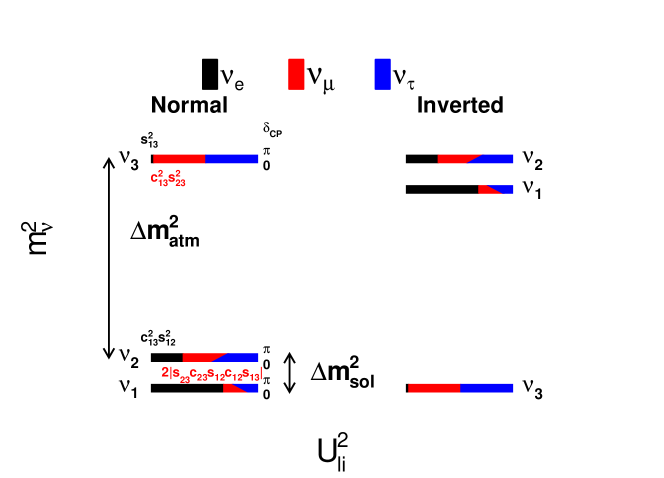
Figure 5: Patterns of neutrino mass and mixing for the normal (left) and inverted (right) hierarchy following Ref. [85]. The best-fit values of neutrino mixing parameters in Ref. [86] are used, which results in slightly different decompositions of the mass eigenstates in terms of flavor eigenstates depending on the mass hierarchy. $\Delta m^{2}_{sol}=\Delta m^{2}_{21}$ and $\Delta m^{2}_{atm}=|\Delta m^{2}_{32}|\approx|\Delta m^{2}_{31}|$. The $l$ flavor component in the $i$th mass eigenstate is expressed as $|U^{2}_{li}|$. The magnitude in front of $\cos\delta_{CP}$ is $2|s_{23}c_{23}s_{12}c_{12}s_{13}|$.

Table 3: Neutrino oscillation parameters taken from Ref. [86]. For the atmospheric mass-squared difference ($|\Delta m^{2}_{31}|\approx|\Delta m^{2}_{32}|$), the best fit results for both the normal (NH) and the inverted mass hierarchy (IH) are shown. These values are used in all the following plots, except where noted.

parameter	best fit value $\pm~{}1\sigma$	3$\sigma$ range
$\sin^{2}\theta_{12}$	$0.306^{+0.012}_{-0.012}$	(0.271, 0.345)
$\theta_{12}$ (degrees)	$33.56^{+0.77}_{-0.75}$	(31.38, 35.99)
$\Delta m^{2}_{21}$ $\times 10^{-5}$ eV2	$7.50^{+0.19}_{-0.17}$	(7.03, 8.09)
(NH) $\sin^{2}\theta_{23}$	$0.441^{+0.027}_{-0.021}$	(0.385, 0.635)
(NH) $\theta_{23}$ (degrees)	$41.6^{+1.5}_{-1.2}$	(38.4, 52.8)
(IH) $\sin^{2}\theta_{23}$	$0.587^{+0.020}_{-0.024}$	(0.393, 0.640)
(IH) $\theta_{23}$ (degrees)	$50.0^{+1.1}_{-1.4}$	(38.8, 53.1)
(NH) $\sin^{2}\theta_{13}$	$0.02166^{+0.00075}_{-0.00075}$	(0.01934, 0.02392)
(NH) $\theta_{13}$ (degrees)	$8.46^{+0.15}_{-0.15}$	(7.99, 8.90)
(IH) $\sin^{2}\theta_{13}$	$0.02179^{+0.00076}_{-0.00076}$	(0.01953, 0.02408)
(IH) $\theta_{13}$ (degrees)	$8.49^{+0.15}_{-0.15}$	(8.03, 8.93)
(NH) $\delta_{CP}$ (degrees)	$261^{+51}_{-59}$	(0, 360)
(IH) $\delta_{CP}$ (degrees)	$277^{+40}_{-46}$	(145, 391)
(NH) $\Delta m^{2}_{31}$ $\times 10^{-3}$ eV2	$+2.524^{+0.039}_{-0.040}$	(+2.407, +2.643)
(IH) $\Delta m^{2}_{32}$ $\times 10^{-3}$ eV2	$-2.514^{+0.038}_{-0.041}$	(-2.635, -2.399)

The phenomenon of neutrino flavor oscillation arises because neutrinos are produced and detected in their flavor eigenstates but propagate as a mixture of mass eigenstates. For example, in vacuum, the neutrino mass eigenstates having energy $E$ would propagate as:

$$\frac{d}{dL}\left(\begin{array}[]{c}\nu_{1}(L)\\ \nu_{2}(L)\\ \nu_{3}(L)\end{array}\right)=-i\cdot V\cdot\left(\begin{array}[]{c}\nu_{1}(L)\\ \nu_{2}(L)\\ \nu_{3}(L)\end{array}\right)$$ (12)

$$=-i\left(\begin{array}[]{ccc}\frac{m_{1}^{2}}{2E}&0&0\\ 0&\frac{m_{2}^{2}}{2E}&0\\ 0&0&\frac{m_{3}^{2}}{2E}\end{array}\right)\cdot\left(\begin{array}[]{c}\nu_{1}(L)\\ \nu_{2}(L)\\ \nu_{3}(L)\end{array}\right),$$ (19)

after traveling a distance $L$. The above equation leads to the solution $\nu_{i}(L)=e^{-i\frac{m_{i}^{2}}{2E}\cdot L}\nu_{i}(0)$. Therefore, for a neutrino produced with flavor $l$, the probability of its transformation to flavor $l^{\prime}$ is expressed as:

$$P_{ll^{\prime}}\equiv P(\nu_{l}\rightarrow\nu_{l^{\prime}})=|<\nu_{l^{\prime}}(L)|\nu_{l}(0)>|^{2}$$

$$=\left|\sum_{j}U_{lj}U^{*}_{l^{\prime}j}e^{-i(V_{jj})L}\right|^{2}\hfill$$

$$=\sum_{j}|U_{lj}U^{*}_{l^{\prime}j}|^{2}+\sum_{j}\sum_{k\neq j}U_{lj}U^{*}_{l^{\prime}j}U^{*}_{lk}U_{l^{\prime}k}e^{i\frac{\Delta m^{2}_{jk}L}{2E}},$$ (20)

with $\Delta m^{2}_{jk}=m^{2}_{j}-m^{2}_{k}$. From Eq. (3.1), it is obvious that the two Majorana phases are not involved in neutrino flavor oscillation. In other words, these Majorana phases cannot be determined from neutrino flavor oscillation.

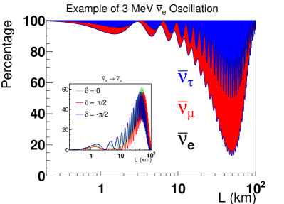
Figure 6: Example of a 3-MeV reactor electron antineutrino oscillation in the three-neutrino framework. The current best estimate of neutrino mixing parameters (tabulated in Table 3) is used. The red and blue bands refer to the oscillation into $\bar{\nu}_{\mu}$ and $\bar{\nu}_{\tau}$ respectively, and the black curve is the $\bar{\nu}_{e}$ disappearance probability in percentages. The inner panel replots the $\bar{\nu}_{\mu}$ appearance probability in percentages, which is in principle sensitive to the unknown CP phase $\delta_{CP}$. However, the energy of the reactor neutrino is less than the $\bar{\nu}_{\mu}$ charged-current interaction threshold. The corresponding CPT-invariant process $\nu_{\mu}\rightarrow\nu_{e}$ is the primary method to measure $\delta_{CP}$ using accelerator neutrinos.

When neutrinos propagate in matter, Eq. (3.1) must be modified because of the additional contribution originating from the interaction between neutrinos and matter constituents. This phenomenon is commonly referred to as the Mikheyev–Smirnov–Wolfenstein (MSW) [87, 88, 89] or matter effect. The modification in oscillation probabilities is a result of the additional contribution of charged-current interaction (W-boson exchange) between electrons in matter with electron neutrinos (antineutrinos). For neutrinos of other flavors (muon and tau), interaction with electron can only proceed via neutral current (Z-boson exchange).

Taking into account the matter effect, we have

$$\frac{d}{dL}\left(\begin{array}[]{c}\nu_{e}(L)\\ \nu_{\mu}(L)\\ \nu_{\tau}(L)\end{array}\right)=-i\left(\begin{array}[]{ccc}V_{C}&0&0\\ 0&0&0\\ 0&0&0\end{array}\right)\cdot\left(\begin{array}[]{c}\nu_{e}(L)\\ \nu_{\mu}(L)\\ \nu_{\tau}(L)\end{array}\right),$$ (21)

where $V_{C}=\sqrt{2}G_{F}N_{e}$ with $G_{F}$ being the Fermi constant and $N_{e}$ being the electron density in matter. The sign of $V_{C}$ is reversed for electron antineutrinos. The propagation matrix $V$ in Eq. (12) is modified as

$$V^{\prime} = \left(\begin{array}[]{ccc}\frac{m_{1}^{2}}{2E}&0&0\\ 0&\frac{m_{2}^{2}}{2E}&0\\ 0&0&\frac{m_{3}^{2}}{2E}\end{array}\right)+U^{*}\cdot\left(\begin{array}[]{ccc}V_{C}&0&0\\ 0&0&0\\ 0&0&0\end{array}\right)\cdot U$$ (28)

$$= U^{*}_{new}\cdot D\cdot U_{new},$$ (29)

where $U$ is the PMNS matrix.

The new matrix $V^{\prime}$ can be expressed as a product of a unitarity matrix $U_{new}$, a diagonal matrix $D$, and $U_{new}^{*}$. The new energy eigenstates of neutrinos are thus $\nu^{\prime}_{j}=\sum_{i}U_{new}^{ij}\cdot\nu_{i}$, and the new mixing matrix connecting the flavor eigenstates and the energy eigenstates becomes $U^{\prime}=U\cdot U^{*}_{new}$. The oscillation probability in Eq. (3.1) can be obtained by substituting the mixing matrix $U$ by $U^{\prime}$ and the mass eigenstates $\nu_{i}$ by the energy eigenstates $\nu^{\prime}_{i}$. For reactor neutrino experiments, this effect is generally small because of low neutrino energies and short baselines. For example, the changes in disappearance probabilities are below 0.006% and 7% for the Daya Bay ($\sim$1.7 km baseline) and KamLAND ($\sim$180 km baseline) experiments, respectively, when the matter effect is taken into account.

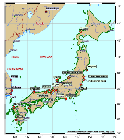
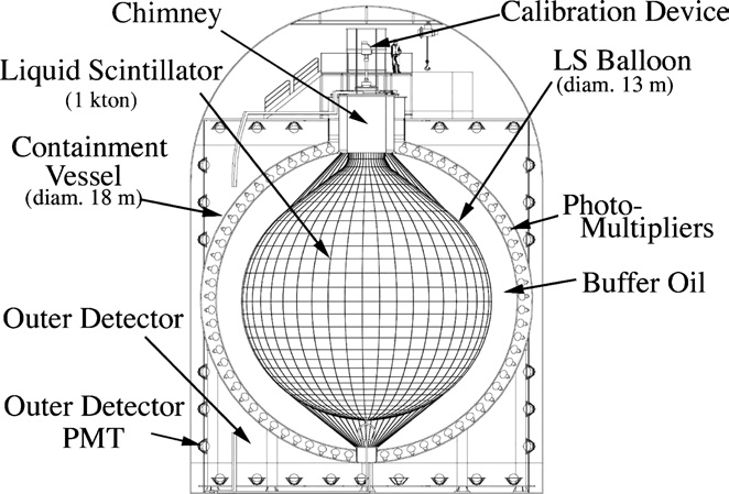
Figure 7: A) The locations of nuclear power plants in Japan, Korea, and Far East Russia from International Nuclear Safety Center at Argonne National Laboratory (http://www.insc.anl.gov/). The KamLAND detector is located at (36.42^∘ N, 137.31^∘ E) in the middle of Japan. B) The structure of the KamLAND detector taken from Ref. [26].

The best values for the parameters obtained from a global fit [86] to neutrino oscillation data after the Neutrino 2016 conference [90] are summarized in Table 3. A comparable result has also been obtained in Ref. [91]. Incremental updates on neutrino oscillation parameters have been presented in the Neutrino 2018 conference [92]. The patterns of neutrino mass and mixing are shown in Fig. 5. Regarding the parameters that can be accessed through neutrino oscillation, two crucial pieces, i) the neutrino mass hierarchy (or the ordering of neutrino masses), which is the sign of $\Delta m^{2}_{32}=m^{2}_{3}-m^{2}_{2}$; and ii) the magnitude of the Dirac charge and parity (CP) phase $\delta_{CP}$, are still missing. Figure 6 shows an example of a 3-MeV reactor electron antineutrino oscillation in the standard three-neutrino framework:

with $\Delta_{ij}\equiv\frac{\Delta m^{2}_{ij}L}{4E}$ and $\delta_{le}=-arg\left(U^{*}_{l3}U_{e3}U_{l2}U^{*}_{e2}\right)$ for lepton flavor $l$. The fast and slow oscillation corresponds to $|\Delta m^{2}_{32}|\approx|\Delta m^{2}_{31}|$ and $\Delta m^{2}_{21}$ mass squared difference, respectively.

3.2 Observation of Neutrino Oscillations in the Solar Sector

The first hint of solar neutrino flavor transformation was Ray Davis’s measurement of the solar $\nu_{e}$ flux using 610 tons of liquid C₂Cl₄, through the reaction $\nu_{e}+^{37}$Cl$\rightarrow e^{-}+^{37}$Ar [93]. Compared with the prediction from the standard solar model (SSM) [94, 95], the measured $\nu_{e}$ flux was only about one-third as large [96, 97]. This result was subsequently confirmed by SAGE [98, 99] and GALLEX [100, 101] using the reaction $\nu_{e}+^{71}$Ga$\rightarrow e^{-}+^{71}$Ge and by Kamiokande [102, 103] and Super-K [104, 105] experiments using $\nu+e^{-}\rightarrow\nu+e^{-}$ elastic scattering. This large discrepancy between measurements and predictions from the SSM was commonly referred to as the ‘solar neutrino puzzle’. While many considered this discrepancy as evidence for the inadequacy of SSM, others suggested neutrino oscillation as the cause.

To solve the ‘solar neutrino puzzle’, the Sudbury Neutrino Observatory (SNO) experiment was performed to measure the total flux of all neutrino flavors from the Sun using three processes: i) the neutrino flux of all flavors from the neutral current (NC) reaction on deuterium from heavy water $\nu_{e,\mu,\tau}+d\rightarrow\nu+p+n$; ii) the $\nu_{e}$ flux through the charged current (CC) reaction $\nu_{e}+d\rightarrow e^{-}+p+p$; and iii) a combination of $\nu_{e}$ and $\nu_{\mu,\tau}$ flux through the elastic scattering (ES) on electrons $\nu+e\rightarrow\nu+e$. The measured flux of all neutrino flavors from the NC channel was entirely consistent with the prediction of SSM [106], while the measured $\nu_{e}$ flux from the CC channel clearly showed a deficit. This result was consistent with neutrino mixing and flavor transformation modified by the matter effect in the Sun.

The solar neutrino data allowed several solutions in the parameter space of the neutrino mixing angle $\theta_{12}$ and the mass squared difference $\Delta m^{2}_{21}$. This ambiguity was the result of several factors, including the relatively large uncertainty of the solar $\nu_{e}$ flux predicted by SSM, the matter effect inside the Sun, and the long distance neutrinos travel to terrestrial detectors. To resolve this ambiguity, a reactor neutrino experiment, the Kamioka Liquid-scintillator ANtineutrino Detector (KamLAND) [26], was constructed in Japan to search with high precision for the $\sim$MeV reactor $\bar{\nu}_{e}$ oscillation at $\sim$200 km. Assuming CPT invariance, KamLAND directly explored the so-called ‘large mixing angle’ (LMA) parameter region suggested by solar neutrino experiments.

As shown in Fig. 7A, the KamLAND experiment was located at the site of the former Kamiokande experiment [103] under the summit of Mt. Ikenoyama in the Japanese Alps. A 2700-m water equivalent (m.w.e.) vertical overburden was used to suppress backgrounds associated with cosmic muons. The experimental site was surrounded by 55 Japanese nuclear reactor cores. Reactor operation information, including thermal power and fuel burn-up, was provided by all Japanese nuclear power plants, allowing KamLAND to calculate the expected instantaneous neutrino flux. The contribution to the total $\bar{\nu}_{e}$ flux from Japanese research reactors and all reactors outside of Japan was about 4.5% [107]. In particular, the contribution from reactors in Korea was estimated at 3.2$\pm$0.3% and from other countries at 1.0$\pm$0.5%. The flux-weighted average $\bar{\nu}_{e}$ baseline was about 180 km, which was well suited to explore the LMA solution.

The schematic layout of the KamLAND detector is shown in Fig. 7B. One kiloton of highly purified LS, 80% dodecane + 20% pseudocumene, was enclosed in a 13-m diameter balloon. The balloon was restrained by ropes inside a mineral-oil buffer that was housed in a 18-m diameter stainless steel (SS) sphere. An array of 554 20-inch and 1325 17-inch PMTs was mounted to detect light produced by the IBD interaction. The SS vessel was then placed inside a purified water pool, which also functioned as an active muon-veto Cerenkov detector. The detector response was calibrated by deployments of various radioactive sources. Resolutions of 12 cm/$\sqrt{E~{}({\rm MeV})}$, 6.5%/$\sqrt{E~{}({\rm MeV})}$, and 1.4% were achieved for the position, energy, and the absolute energy scale uncertainty, respectively.

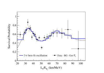
Figure 8: Survival probability of $\bar{\nu}_{e}$ events as a function of $L/E$ in the KamLAND detector [108]. The matter effect is included in the calculation of the survival probability. The dip position of the oscillation ($\sim$50 km/MeV) is consistent with the second oscillation node for $\Delta m^{2}_{21}$. The size of the depletion is a measure of $\sin^{2}2\theta_{12}$.

Given the long baselines between the detector and the reactors, KamLAND expected to observe about one reactor IBD event every day. The IBD events were selected by requiring less than 1 ms time difference and 2-meter distance between the prompt and delayed signals. The latter is a 2.2-MeV $\gamma$ ray from neutron capture on hydrogen (see Table 2). To reduce the accidental coincidence backgrounds from external radioactivities, the IBD selection was restricted to the innermost 6-m radius LS region. With the additional information of the event energy, position, and time, the accidental background was suppressed to $\sim$5% of the IBD signal. The dominant background ($\sim$10%) was from the $\alpha+^{13}$C$\rightarrow n+^{16}$O reaction ($\alpha-n$ background). The incident $\alpha$ is from the decay of ²¹⁰Po, a decay product of ²²²Rn with a half-life of 3.8 days. A decay product of uranium, ²²²Rn is commonly found in air and many materials as a trace element. The prompt signal came from either a neutron scattering off a proton or ¹⁶O de-excitation, and the delayed neutron capture signal mimicked a $\bar{\nu}_{e}$ IBD event. Additional backgrounds included i) the geoneutrinos produced in the decay chains of ²³²Th and ²³⁸U inside the earth, which is an active research area by itself [109, 110]; ii) cosmogenic ⁹Li or ⁸He through $\beta$ decay accompanied by a neutron emission; iii) fast neutrons produced from muons interacting with the nearby rocks; and iv) atmospheric neutrinos.

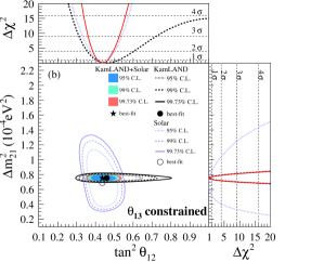
Figure 9: Allowed regions projected in the (tan${}^{2}\theta_{12}$, $\Delta m^{2}_{21}$) plane, for solar and KamLAND data from a three-flavor oscillation analysis [108]. The shaded regions are from a combined analysis of the solar and KamLAND data. The side panels show the $\Delta\chi^{2}$-profiles projected onto the tan${}^{2}\theta_{12}$ and $\Delta m^{2}_{21}$ axes. For this result, the value of $\theta_{13}$ is constrained by the results from reactor experiments with $\sim$km baselines.

The KamLAND experiment [26, 107, 111] clearly observed the oscillation of reactor neutrinos and unambiguously established LMA as the solution of the solar neutrino puzzle. The latest KamLAND result [108] is shown in Fig. 8 as a function of $L/E_{\nu}$, where an oscillatory pattern covering three oscillation extrema is clearly observed. Figure 9 shows $\Delta m^{2}_{21}$ vs. $\tan^{2}\theta_{12}$ from KamLAND and solar neutrino experiments.

While the solar neutrino experiments are more sensitive to the mixing angle $\theta_{12}$, KamLAND measures the mass-squared difference $\Delta m^{2}_{21}$ more accurately through fitting the spectral distortions. The observation of consistent mixing parameters with two distinct neutrino sources (solar vs. reactor neutrinos) and two different physics mechanisms (flavor transformation with the matter effect vs. flavor oscillation in vacuum) provides compelling evidence for non-zero neutrino mass and mixing.

Besides contributing to the measurement of neutrino mass and mixing parameters in the solar sector, the KamLAND data also gave an early hint of a non-zero $\theta_{13}$ [112]. With $\theta_{13}=0$, the data from KamLAND [111] favors a larger value of $\theta_{12}$ as compared to that from the SNO solar neutrino data [113]. This small difference in $\theta_{12}$ can be reduced for a non-zero value of $\theta_{13}$ ($\theta_{13}>0$ at $\sim$1.2$\sigma$ level) [112]. In the next section, we review the discovery of a non-zero $\theta_{13}$.

3.3 Discovery of a Non-zero $\theta_{13}$

Table 4: Key parameters of five past and present reactor $\theta_{13}$ experiments, including the reactor thermal power (in giga-watts), distance to reactors, target mass and material of the detectors, and overburden of the underground site (in meter-water-equivalent). PC, PXE, and LAB stands for Pseudocumene, Phenylxylylethane, and Linear Alkybenzene for liquid scintillator (LS) materials, respectively.

Experiment	Power	Baseline	Target Material	Mass	Overburden
	(GWth)	(m)	Gd-doped LS	(tons)	(m.w.e.)
CHOOZ	8.5	1050	paraffin-based	5	300
Palo Verde	11.6	750-890	(segmented) PC-based	12	32
Double Chooz	8.5	400	PXE-based	8	120
		1050		8	300
RENO	16.8	290	LAB	16	120
		1380		16	450
Daya Bay	17.4	360	LAB	$2\times 20$	250
		500		$2\times 20$	265
		1580		$4\times 20$	860

3.3.1 History of Searching for a Non-zero $\theta_{13}$

As introduced in Sec. 3.1, three mixing angles, one phase, and two independent mass-squared differences govern the phenomenon of neutrino flavor oscillation. KamLAND and solar neutrino experiments determined $\theta_{12}\approx$ 33^∘ and $\Delta m^{2}_{21}\approx$ 7.5$\times 10^{-5}~{}{\rm eV}^{2}$. Meanwhile, the results $\theta_{23}\approx 45^{\circ}$ and $|\Delta m^{2}_{32}|\approx$ 2.3$\times 10^{-3}~{}{\rm eV}^{2}$ came from atmospheric neutrino experiments such as Super-K [30] and long-baseline disappearance experiments, including K2K [114], MINOS [114], T2K [115], and NO$\nu$A [116]. In particular, the zenith-angle dependent deficit of the upward-going atmospheric muon neutrinos reported by the Super-K experiment [30] in 1998 was the first compelling evidence of neutrino flavor oscillation. Given that both the $\theta_{23}$ and $\theta_{12}$ angles are large, it is natural to expect that the third mixing angle $\theta_{13}$ is also sizable.

There are at least two ways to access $\theta_{13}$. The first is to use reactor neutrino disappearance $P\left(\bar{\nu}_{e}\rightarrow\bar{\nu}_{e}\right)$ (see Eq. LABEL:eq:3f_osc). For a detector located at a distance $L$ near the first maximum of $\sin^{2}\Delta_{31}$, the amplitude of the oscillation gives $\sin^{2}2\theta_{13}$. The second method is to use accelerator muon neutrinos to search for electron neutrino appearance $P\left(\nu_{\mu}\rightarrow\nu_{e}\right)\equiv P\left(\bar{\nu}_{e}\rightarrow\bar{\nu}_{\mu}\right)$ (see Eq. LABEL:eq:3f_osc). In this case, the amplitude of the oscillation depends not only on $\theta_{13}$, but also on several parameters, including $\theta_{23}$, the unknown CP phase $\delta_{CP}$, and neutrino mass hierarchy (through the matter effect in Earth). While the second method can access several important neutrino parameters, the first method provides a direct and unambiguous measurement of $\theta_{13}$.

Historically, the CHOOZ [31, 32] and Palo Verde [33] experiments made the first attempts to determine the value of $\theta_{13}$ in the late 1990s to early 2000s. Both experiments utilized reactor neutrinos to search for oscillation of $\bar{\nu}_{e}$ at baselines of $\sim$1 km using a single-detector configuration. The CHOOZ experiment was located at the CHOOZ power plant in the Ardennes region of France. The CHOOZ detector mass was about 5 tons, and the distance to reactor cores was about 1050 m. The data-taking started in April 1997 and ended in July 1998.

The Palo Verde experiment was located at the Palo Verde Nuclear Generating Station in the Arizona desert of the United States. The Palo Verde detector mass was about 12 tons, and the distances to three reactor cores were 750 m, 890 m, and 890 m. The data-taking started in October 1998 and ended in July 2000. No oscillation were observed in either experiment, and a better upper limit of sin${}^{2}2\theta_{13}<0.12$ was set at 90% confidence level (C.L.) by CHOOZ.

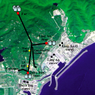
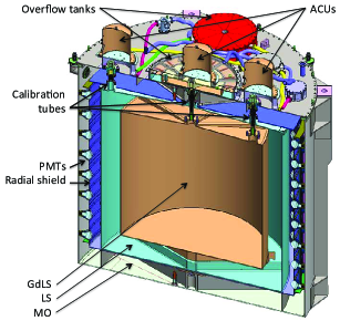
Figure 10: A) The layout and the map of the Daya Bay experiment and the hosting Daya Bay plant campus. B) The structure of the Daya Bay antineutrino detector (AD), taken from Ref. [40]. The Daya Bay ADs were equipped with three automated calibration units (ACUs), two for the Gd-LS volume and one for the LS volume.

Given the measured values of $\theta_{12}$ and $\theta_{23}$ and the null $\theta_{13}$ results from CHOOZ and Palo Verde, several phenomenological models of neutrino mixing patterns, such as bimaximal and tribimaximal mixing [117, 118], became popular. In these models, the neutrino mass matrix in the flavor basis,

$$M_{\nu}=U\cdot M_{\nu}^{diag}\cdot U^{{\dagger}},$$ (33)

is constructed based on flavor symmetries , and $\theta_{13}$ was predicted to be either zero or very small. Therefore, a new generation of reactor experiments (Double Chooz, Daya Bay, and RENO) was designed to search for a small non-zero $\theta_{13}$. To suppress reactor- and detector-related systematic uncertainties, all three experiments adopted the ratio method advocated in Ref. [119] , which required placing multiple identical detectors at different baselines. Table 4 summarizes the key parameters for past and present reactor $\theta_{13}$ experiments.

In 2011, almost 10 years after CHOOZ and Palo Verde, several hints collectively suggested a non-zero $\theta_{13}$ [120]. The first one was based on a small discrepancy between KamLAND and the solar neutrino measurements [112]. Subsequently, accelerator neutrino experiments MINOS [121] and T2K [122] reported their search for $\nu_{\mu}$ to $\nu_{e}$. In particular, T2K disfavored the $\theta_{13}$ = 0 hypothesis at 2.5$\sigma$ [122].

In early 2012, the Double Chooz reactor experiment reported that the $\theta_{13}$ = 0 hypothesis was disfavored at 1.7$\sigma$, based on their far-detector measurement [36]. These hints of a non-zero $\theta_{13}$ culminated in March 2012, when the Daya Bay reactor neutrino experiment reported the discovery of a non-zero $\theta_{13}$ with a 5.1$\sigma$ significance [34].

About one month later, RENO confirmed Daya Bay’s finding of a non-zero $\theta_{13}$ with a 4.9$\sigma$ significance [35]. Later in 2012, Daya Bay increased the significance to 7.7$\sigma$ using a larger data set [123]. A non-zero $\theta_{13}$ was firmly established. In the following, we review three reactor $\theta_{13}$ experiments: Daya Bay, RENO, and Double Chooz. Since these three experiments had many similarities in their design and physics analysis, we use Daya Bay to illustrate some common features.

3.3.2 The Daya Bay Reactor Neutrino Experiment

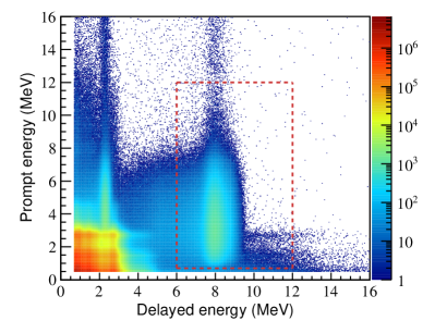
Figure 11: The distribution of prompt versus delayed energy for signal pairs which satisfied the $\bar{\nu}_{e}$ inverse beta decay selection criteria, taken from Ref. [124]. A few-percent contamination from accidental backgrounds (symmetric under interchange of prompt and delayed energy) and ⁹Li decay and fast neutron backgrounds (high prompt and $\sim$8 MeV delayed energy) are visible within the selected region. Inverse beta decay interactions where the neutron was captured on hydrogen provided an additional signal region with delayed energy around 2.2 MeV, albeit with much higher background.

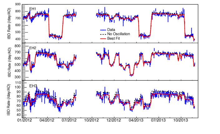
Figure 12: Daily averaged rates of IBD candidate events per detector in three experimental halls of Daya Bay as a function of time. The dotted curves represent no-oscillation predictions. The rates predicted with the best-fit non-zero $\sin^{2}2\theta_{13}$ are shown as the red solid curves. The plot is taken from Ref. [125].

The Daya Bay Reactor Neutrino Experiment was located on the campus of the Daya Bay nuclear reactor power plant in southern China. As shown in Fig. 10A, the plant hosted six reactor cores whose locations were grouped into three clusters: the Daya Bay, Ling Ao, and Ling Ao II clusters. The total thermal power was about 17.4 GW. To monitor antineutrino flux from the three reactor clusters, near-detector sites were implemented. Two near-detector sites: the Daya Bay site ($\sim$363 m from the Daya Bay cluster) and the Ling Ao site ($\sim$500 m from the Ling Ao and Ling Ao II clusters) were constructed. The locations of the near and far sites were chosen to maximize the sensitivity to $\theta_{13}$. In particular, the Ling Ao near site and the far site were both located at approximately equal distances from the Ling Ao and Ling Ao II clusters, largely reducing the effect of antineutrino flux uncertainties from these two clusters. The average baseline of the far site was $\sim$1.7 km.

Each near underground site hosted two antineutrino detectors (ADs). The far site hosted four ADs that pair with the four ADs of the two near sites, providing a maximal cancellation of detector effects. The effective vertical overburdens were 250, 265, and 860 m.w.e. for the Daya Bay site (EH-1), the Ling Ao site (EH-2), and the far site (EH-3), respectively. With the near- and far-sites configuration, the contribution from reactor flux uncertainties was suppressed by a factor of 20 [123], which was the best among the reactor $\theta_{13}$ experiments.

Figure 10B shows the schematic view of an AD [126, 127]. The innermost region was filled with 20 tons of Gd-doped linear-alkylbenzene-based liquid scintillator (LAB GdLS). An array of 192 8-inch PMTs was installed on each AD. Three automated calibration units (ACUs) [128] were equipped to periodically calibrate the detector response. Similar to KamLAND, ADs were placed inside high-purity water pools to reduce radioactive backgrounds from the environment. With PMTs installed, the water pool was also operated as an independent water Cerenkov detector to veto cosmic muons [129, 130]. Each water pool was further split into two sub-detectors, so that the efficiency in each sub-detector could be cross calibrated. A plane of resistive plate chambers (RPC) was installed on the top of each water pool as an active muon veto.

Figure 13: Reconstructed positron energy spectra for the $\bar{\nu}_{e}$ candidate interactions (black points) from Daya Bay [124]. The spectra of the detectors in each experimental hall are combined: EH1 (top), EH2 (middle), and EH3 (bottom). The measurements are compared with the prediction assuming no oscillation (blue line) and the best-fit three-flavor neutrino oscillation model (red line). The inset in semi-logarithmic scale shows the backgrounds. The ratio of the background-subtracted spectra to prediction assuming no oscillation is shown in the panel beneath each energy spectrum.

Figure 11 shows the distribution of prompt versus delayed energy for signal pairs satisfied the $\bar{\nu}_{e}$ selection criteria, which included a crucial cut on the time difference between the prompt and delayed signals (1 $<\Delta t<$ 200 $\mu$s). Five sources of backgrounds were identified. Ordering them in terms of their magnitudes at the near halls, they were accidental coincidence background, $\beta$-n decays from cosmogenic ⁹Li and ⁸He, fast neutrons produced by untagged muons, correlated $\gamma$-rays from Am-C neutron calibration units [131], and background from the $(\alpha,n)$ reactions [124]. The accidental coincidence background was evaluated with high precision. Two of the three Am-C sources were removed during the 8-AD period for background reduction. Using information from the muon veto system, the fast neutron background rate was well determined. The total backgrounds accounted for $\sim$3% (2%) of the IBD candidate sample in the far (near) sites before the background subtraction.

Table 5: Summary of major systematic uncertainties included in the Daya Bay oscillation analysis [124].

Source	Uncertainty	Correlation
Reactor flux
Fission fractions	5%	Correlation among isotopes from Ref. [132],
		correlated among reactors
Average energy per fission	Uncertainties from Ref. [133]	Correlated among reactors
$\bar{\nu}_{e}$ flux per fission	Huber–Mueller model[46, 47]	Correlated among reactors
Non-equilibrium $\bar{\nu}_{e}$ emission	30% (rel.)	Uncorrelated among reactors
Spent nuclear fuel	100% (rel.)	Uncorrelated among reactors
Reactor power	0.5%	Uncorrelated among reactors
Detector response
Absolute energy scale	$<$1%	Correlated among detectors
Relative energy scale	0.2%	Uncorrelated among detectors
Detector efficiency	0.13%	Uncorrelated among detectors
		partial correlated (0.54 correlation coefficient)
		with relative energy scale
IAV thickness	4% below 1.25 MeV (rel.)	Uncorrelated among detectors
	0.1% above 1.25 MeV
Background
Accidental rate	1% (rel.)	Uncorrelated among detectors
9Li-8He rate	44% (rel.)	Correlated among same-site detectors
Fast neutron rate	13–17% (rel.)	Correlated among same-site detectors
241Am-13C rate	45% (rel.)	Correlated among detectors
($\alpha$,n) rate	50% (rel.)	Uncorrelated among detectors

Since the measurement of oscillation effect was obtained through the comparison of rate and spectra between near and far detectors, the identically designed detectors facilitated a near complete cancellation of the correlated detector systematic uncertainties. The accuracy of the oscillation parameters was thus governed by the uncertainties uncorrelated among detectors. Table 5 summarizes the systematic uncertainties included in the Daya Bay oscillation analysis [124]. In particular, the nature of each uncertainty (correlated or uncorrelated among reactors or detectors) is explicitly listed. For the $\theta_{13}$ determination, an uncorrelated 0.1% uncertainty from the hydrogen-to-Gd neutron capture ratio, which was related to the Gd concentrations in GdLS for all detectors, and an uncorrelated 0.08% uncertainty from the 6-MeV cut on the delayed signal, which depended on the energy scale established in all detectors, were the major uncorrelated uncertainties.

In earlier reactor neutrino experiments, measurements with reactor power on and off provided a powerful tool to separate neutrino signals from backgrounds. While this tool is not applicable in Daya Bay, a clear correlation between the rates of IBD candidate events and the reactor power was observed. Figure 12 shows the daily averaged rates of IBD candidate events at the three experimental halls versus time. The IBD rates exhibit patterns that track well with the variation of effective reactor power viewed at each hall. These data show that the IBD candidate events originate predominantly from the reactors rather than from cosmogenic and radioactive backgrounds.

Based on $\bar{\nu}_{e}$ data from all eight detectors collected in 1230 days, Daya Bay determined $\sin^{2}2\theta_{13}=0.0850\pm 0.0030~{}(stat.)\pm 0.0028~{}(syst.)$ in a rate-only analysis [124], with $|\Delta m^{2}_{32}|$ constrained by atmospheric and accelerator neutrino experimental results. The measured non-zero value of $\sin^{2}2\theta_{13}$ was only about 30% below the upper limit set by the previous CHOOZ experiment.

Prior to the discovery of a non-zero $\theta_{13}$, the only method to measure the mass-squared difference $|\Delta m^{2}_{32}|$ was through muon (anti)neutrino disappearance in atmospheric or accelerator neutrino experiments. Given the IBD spectrum covering the antineutrino energy range from 1.8 MeV to $\sim$8 MeV, the “large” value of $\theta_{13}$ offered an alternative way to precisely measure this quantity.

The first-ever extraction of $|\Delta m^{2}_{ee}|:=|\cos^{2}\theta_{12}\Delta m^{2}_{31}+\sin^{2}\theta_{12}\Delta m^{2}_{32}|$ [134] was made by Daya Bay [135] through probing the relative spectral distortion measured between the near and far detectors. In addition to the various systematic uncertainties in the previous rate analysis, the absolute detector energy response was another important ingredient to extract $|\Delta m^{2}_{ee}|$, since the spectral distortion depended on $\Delta m^{2}_{ee}\frac{L}{E_{\nu}}$. A physics-based energy model was constructed and constrained by calibrations using various $\gamma$-ray sources and the well-known ¹²B beta decay spectrum [124].

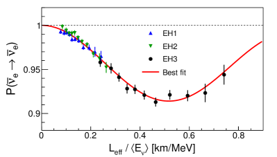
Figure 14: The measured $\bar{\nu}_{e}$ disappearance probability as a function of $L/E$ from Daya Bay [124]. The oscillation amplitude corresponds to $\sin^{2}2\theta_{13}=0.0841\pm 0.0027~{}(stat.)\pm 0.0019~{}(syst.)$. The oscillation frequency corresponds to $|\Delta m^{2}_{ee}|=2.50\pm 0.06~{}(stat.)\pm 0.06~{}(syst.)\times 10^{-3}$ eV².

Figure 13 shows reconstructed positron energy spectra for the IBD candidate events from Daya Bay [124]. The best fit curve corresponds to $\sin^{2}2\theta_{13}=0.0841\pm 0.0027~{}(stat.)\pm 0.0019~{}(syst.)$ and $|\Delta m^{2}_{ee}|=2.50\pm 0.06~{}(stat.)\pm 0.06~{}(syst.)\times 10^{-3}$ eV² [124]. Figure 14 shows the measured $\bar{\nu}_{e}$ disappearance probability as a function of $L/E_{\nu}$. As shown in Fig. 15, improved measurements were reported at the Neutrino 2018 conference [92]. Another benefit of the ‘large’ value of $\theta_{13}$ is that a different sample of the IBD events using neutron capture on hydrogen (nH) in both the GdLS and LS regions can also be employed to independently measure $\theta_{13}$. Since the oscillation signal is large, many systematic associated with the nH channel, which are generally larger than those of the nGd channel, become less important. The details of extracting $\theta_{13}$ using the nH channel from Daya Bay can be found in Ref. [136, 73].

3.3.3 The RENO and Double Chooz Experiments

The Reactor Experiment for Neutrino Oscillation (RENO) was a short-baseline reactor neutrino experiment built near the Hanbit nuclear power plant in South Korea. Like the Daya Bay experiment, RENO was designed to measure the mixing angle $\theta_{13}$. The six reactor cores in RENO had a total thermal power of 16.4 GW. The reactor cores were equally spaced in a straight line, with the near and far detector sites located along a line perpendicular to and bisecting the reactor line. The near site was $\sim$290 m from the geometric center of reactor cores, while the far site, located on the opposite side of the reactor line, was at a distance of $\sim$1380 m. Because of the large variation in the distances between the near detector and various reactor cores, the suppression of the uncertainty in the reactor neutrino flux was less than ideal. Taking a similar approach as Daya Bay, RENO adopted a three-zone LS antineutrino detector nested in a muon veto system. The central target zone contained 16 tons of 0.1% Gd-doped LAB LS. A total of 354 10-inch PMTs were mounted on the inner wall and the top and bottom surfaces of a stainless steel container. Unlike Daya Bay, RENO had one detector in each experimental site.

RENO started data taking in both the near and far detectors in the summer of 2011, ahead of all competing experiments. The first RENO $\theta_{13}$ result was published in Ref. [35] in 2012. This result was in agreement with Daya Bay’s finding of a non-zero $\theta_{13}$ [34] with a near-5$\sigma$ confidence level. The observation of a 4 MeV–6 MeV anomaly in the prompt energy spectrum, which is discussed in detail in Sec. 4.3, was first reported by RENO [137]. Most recently, RENO also reported a measurement of $|\Delta m^{2}_{ee}|$ from the antineutrino energy spectral distortion [138], which was consistent with world measurements. Figure 15 shows RENO’s latest results on $\sin^{2}2\theta_{13}$ and $|\Delta m^{2}_{ee}|$, reported at the Neutrino 2018 conference [92]. In particular, the first measurement of $|\Delta m^{2}_{ee}|$ using the nH channel was performed.

Double Chooz built upon the former CHOOZ experiment that set the best upper limit of $\sin^{2}2\theta_{13}$ prior to the discovery of a non-zero $\theta_{13}$. It added a near site detector at a distance of $\sim$410 m with a 115-m.w.e. overburden. The far site was the original CHOOZ detector site, having a 1067 m baseline and a 300-m.w.e. overburden. The total thermal power of the two Double Chooz reactors was 8.7 GW. Based on the original CHOOZ design, Double Chooz adopted the three-zone design. Instead of LAB-based LS, Double Chooz’s central target region was a 10-ton PXE-based LS. For each detector, 390 low-background 10-inch PMTs were mounted on the inner surfaces of the stainless steel container. Unlike Daya Bay, Double Chooz had one detector in each experimental site. Because of a construction delay, the first result of Double Chooz [36, 139], a 1.7$\sigma$ hint of a non-zero $\theta_{13}$, included only the far-site data. To constrain the reactor neutrino flux uncertainty, Double Chooz used the Bugey-4 measurement [140] to normalize the flux. The systematic uncertainties of the first result were subsequently improved, as reported in Ref. [141], with backgrounds constrained by the reactor-off data. An improved measurement of $\theta_{13}$ with about twice the antineutrino flux exposure was reported in Ref. [142]. Double Chooz carried out the first independent $\theta_{13}$ analysis using the neutron-capture-on-hydrogen data [143, 144]. The Double Chooz near detector started taking data in 2014. The latest Double Chooz result using both near and far detector data yielded $\sin^{2}2\theta_{13}=0.105\pm 0.014$ [92].

3.3.4 Impacts of a Non-zero $\theta_{13}$

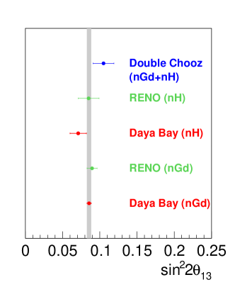
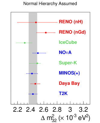
Figure 15: Global results on $\theta_{13}$ (A) and $\Delta m^{2}_{32}$ (B) taken from the results presented at the Neutrino 2018 conference [92]. For $\Delta m^{2}_{32}$, only results of the normal hierarchy are shown.

Figure 15 summarizes the status of $\theta_{13}$ and $|\Delta m^{2}_{32}|$ after the Neutrino 2018 conference [92]. The precision of $\sin^{2}2\theta_{13}$ from Daya Bay was better than 3.5%, making it the best measured mixing angle. Given the relatively ‘large’  value of $\theta_{13}$, the $|\Delta m^{2}_{32}|$ was measured precisely using reactor neutrinos, given the well-controlled systematics for the detector and the antineutrino flux. In particular, the precision of $|\Delta m^{2}_{32}|$ from Daya Bay had reached a similar precision as those from accelerator neutrino and atmospheric neutrino experiments, as shown in Fig. 15.

Besides the precision measurement of $|\Delta m^{2}_{32}|$, a non-zero $\theta_{13}$ also opens up many opportunities for future discoveries. In particular, it allows for a determination of the neutrino mass hierarchy in a medium-baseline reactor neutrino experiment, which is elaborated in Sec. 3.4. In addition, it enables the search for CP violation in the leptonic sector, as well as the determination of the neutrino mass hierarchy through precision (anti-)$\nu_{\mu}\rightarrow$ (anti-)$\nu_{e}$ oscillation in accelerator neutrino experiments (see Ref. [145] for a recent review). To leading order in $\alpha=\Delta m^{2}_{21}/\Delta m^{2}_{31}$, the probability of the $\nu_{\mu}\rightarrow\nu_{e}$ oscillation can be written as [146]:

$$P(\nu_{\mu}\rightarrow\nu_{e}) = \sin^{2}\theta_{23}\frac{\sin^{2}2\theta_{13}}{(A-1)^{2}}\sin^{2}[(A-1)\Delta_{31}]\hfill$$ (34)

$$+ \alpha^{2}\cos^{2}\theta_{23}\frac{\sin^{2}2\theta_{12}}{A^{2}}\sin^{2}(A\Delta_{31})\hfill$$

$$- \alpha\frac{\sin 2\theta_{12}\sin 2\theta_{13}\sin 2\theta_{23}\cos\theta_{13}\sin\delta_{CP}}{A(1-A)}$$

$$\times \sin\Delta_{31}\sin(A\Delta_{31})\sin[(1-A)\Delta_{31}]\hfill$$

$$+ \alpha\frac{\sin 2\theta_{12}\sin 2\theta_{13}\sin 2\theta_{23}\cos\theta_{13}\cos\delta_{CP}}{A(1-A)}$$

$$\times \cos\Delta_{31}\sin(A\Delta_{31})\sin[(1-A)\Delta_{31}],\hfill$$

where

$$\Delta_{ij} = \Delta m^{2}_{ij}L/4E_{\nu},$$

$$A = \sqrt{2}G_{F}N_{e}2E_{\nu}/\Delta m^{2}_{31}.$$ (35)

For antineutrinos, the signs of $\delta_{CP}$ and $A$ are reversed. The sensitivity to the mass hierarchy (i.e., the sign of $A$) mainly comes from the first term in Eq. (34), which becomes non-zero for a non-zero $\theta_{13}$. In addition, the sensitivity to the mass hierarchy is larger for a larger value of $\theta_{13}$. Similarly, the sensitivity to CP violation (i.e., a non-zero value for $\sin\delta_{CP}$) comes from the last two terms, which are in play for a non-zero $\theta_{13}$. In contrast to the mass hierarchy sensitivity, the sensitivity to CP violation is approximately independent of the value of $\theta_{13}$ [147]. To illustrate this point, we use the fractional asymmetry

$$A^{\mu e}_{CP}\equiv\frac{({P(\nu_{\mu}\to\nu_{e})-P(\bar{\nu}_{\mu}\to\bar{\nu}_{e})})}{({P(\nu_{\mu}\to\nu_{e})+P(\bar{\nu}_{\mu}\to\bar{\nu}_{e})})}.$$ (36)

At larger values of $\theta_{13}$, $A^{\mu e}_{CP}\sim$1/$\sin 2\theta_{13}$ becomes smaller for a given value of CP phase. However, the increase in the number of events leads to a better measurement of $A^{\mu e}_{CP}$, with statistical uncertainties $\delta A^{\mu e}_{CP}\sim$1/$\sin 2\theta_{13}$. These two effects approximately cancel each other. In real experiments, a larger value of $\theta_{13}$ is actually favored, as the impact of various backgrounds on the $\nu_{\mu}\rightarrow\nu_{e}$ signal is reduced with larger signal strength.

By 2020, the precision of $\sin^{2}2\theta_{13}$ and $\Delta m^{2}_{32}$ in Daya Bay is projected to be better than 3%. The comparison of the $\theta_{13}$ measurement from reactor $\bar{\nu}_{e}\rightarrow\bar{\nu}_{e}$ disappearance and that from the accelerator $\nu_{\mu}\rightarrow\nu_{e}$ appearance in the future DUNE [148] and Hyper-K [149] experiments will provide one of the best unitarity tests of the PMNS matrix [150].

3.4 Future Opportunities

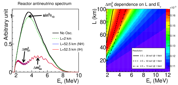
Figure 16: A) Expected antineutrino energy spectra at different baselines with $\Delta m^{2}_{ee}=2.41\times 10^{-3}$ eV². The effects of a non-zero $\sin^{2}2\theta_{13}$ and different MHs are emphasized. B) $\Delta m^{2}_{\phi}$ is shown as a function of the neutrino energy and the baseline. At 50 km–60 km, the $\Delta m^{2}_{\phi}$ shows a clear dependence on the neutrino energy. Such a dependence is the key to determine the MH. The plot is taken from Ref. [151].

3.4.1 Determination of the Neutrino Mass Hierarchy

The neutrino mass hierarchy (MH), i.e., whether the third generation neutrino mass eigenstate is heavier or lighter than the first two, is one of the remaining unknowns in the minimal extended $\nu$SM (see Ref. [152] for a recent review) . The determination of the MH, together with searches for neutrinoless double beta decay, may reveal whether neutrinos are Dirac or Majorana fermions, which could significantly advance our understanding of the Universe.

The precise measurement of $\sin^{2}2\theta_{13}$ by the current generation of short-baseline reactor neutrino experiments has provided a unique opportunity to determine the MH in a medium-baseline ($\sim$55 km) reactor neutrino experiment [151, 153, 154, 155, 156, 157, 158, 159]. The oscillation from the atmospheric mass-squared difference manifests itself in the energy spectrum as multiple cycles that contain the MH information, as shown in the following formula derived from Eq. (LABEL:eq:3f_osc):

$$P_{\bar{\nu}_{e}\rightarrow\bar{\nu}_{e}} = 1-2s_{13}^{2}c_{13}^{2}-4c_{13}^{2}s_{12}^{2}c_{12}^{2}\sin^{2}\Delta_{21}$$

$$+ 2s_{13}^{2}c_{13}^{2}\sqrt{1-4s_{12}^{2}c_{12}^{2}\sin^{2}\Delta_{21}}\cos(2|\Delta_{32}|\pm\phi),$$

where $\Delta_{21}\equiv\Delta m_{21}^{2}L/4E$, $\Delta_{32}\equiv\Delta m_{32}^{2}L/4E$, and

$$\sin\phi=\frac{c_{12}^{2}\sin 2\Delta_{21}}{\sqrt{1-4s_{12}^{2}c_{12}^{2}\sin^{2}\Delta_{21}}}\,,$$

$$\cos\phi=\frac{c_{12}^{2}\cos 2\Delta_{21}+s_{12}^{2}}{\sqrt{1-4s_{12}^{2}c_{12}^{2}\sin^{2}\Delta_{21}}}.$$

The $\pm$ sign in the last term of Eq. (3.4.1) depends on the MH: the plus sign indicates the normal hierarchy (NH) and the minus sign indicates the inverted hierarchy (IH). The principle of determining MH through spectral distortion can be understood from Fig. 16B, which shows the energy and baseline dependent $\Delta m^{2}_{\phi}:=4E\cdot\phi/L$, based on Eq. (3.4.1). The three lines represent three different choices of energy resolution. In the region left of the line, the measurement of $\Delta m^{2}_{\phi}$ is compromised. Above $\sim$40 km, $\Delta m^{2}_{\phi}$ possesses a clear energy dependence. In particular, at $\sim$50 km, $\Delta m^{2}_{\phi}$ at low-energy region (2 MeV–4 MeV) is larger than that at high-energy region (4 MeV–8 MeV). This distinction provides an excellent opportunity to determine the MH. For NH, the $\Delta m^{2}_{eff}:=2|\Delta m^{2}_{32}|+\Delta m^{2}_{\phi}$ measured in the low-energy region (2 MeV–4 MeV) would be higher than that measured in the high-energy region (4 MeV–8 MeV). In comparison, for the IH, the $\Delta m^{2}_{eff}:=2|\Delta m^{2}_{32}|-\Delta m^{2}_{\phi}$ measured in the low-energy region would be lower than that measured at high energy. Figure 16A shows the reactor neutrino energy spectra at a baseline of 52.5 km for both NH and IH. The choice of MH leads to a shift in the oscillation pattern at low-energy region relative to that at high-energy region.

The Jiangmen Underground Neutrino Observatory (JUNO) [37] is a next-generation (medium-baseline) reactor neutrino experiment under construction in Jiangmen City, Guangdong Province, China. It consists of a 20-kton underground LS detector having a 1850 m.w.e. overburden and two reactor complexes at baselines of $\sim$53 km, with a total thermal power of 36 GW. With $\sim$100k IBD events from reactor neutrinos (about six years data-taking), JUNO aims to determine the MH at 3$\sigma$ sensitivity.  This goal in sensitivity relies on an unprecedented 3%/$\sqrt{E~{}\rm(MeV)}$ energy resolution, which requires a $\sim$80% photo-cathode coverage, an increase in both LS light yield and attenuation length, and an increase in PMT quantum efficiency. In addition, excellent control of the energy-scale uncertainty [151, 159, 162] is crucial.

3.4.2 Precision Measurements of Neutrino Mixing Parameters

In addition to determining the MH, JUNO will access four fundamental neutrino mixing parameters: $\theta_{12}$, $\theta_{13}$, $\Delta m^{2}_{21}$, and $|\Delta m^{2}_{32}|$. JUNO is expected to be the first experiment to observe neutrino oscillation simultaneously from both atmospheric and solar neutrino mass-squared differences and will be the first experiment to observe more than two oscillation cycles of the atmospheric mass-squared difference. Moreover, JUNO is expected to achieve better than 1% precision measurements of $\sin^{2}2\theta_{12}$, $|\Delta m^{2}_{32}|$, and $\Delta m^{2}_{21}$, which provides very powerful tests of the standard three-flavor neutrino model. In particular, the precision measurement of $\sin^{2}2\theta_{12}$ will lay the foundation for a future sub-1% direct unitarity test of the PMNS matrix $U$.

The combination of short-baseline reactor neutrino experiments (such as Daya Bay, RENO, and Double Chooz), medium-baseline reactor neutrino experiments (such as KamLAND and JUNO), and solar neutrino experiments (such as SNO) enable the first direct unitarity test of the PMNS matrix [150, 163]: $|U_{e1}|^{2}+|U_{e2}|^{2}+|U_{e3}|^{2}\stackrel{{\scriptstyle?}}{{=}}1$. When combined with results from Daya Bay and SNO, JUNO’s precision measurement will test this unitarity condition to 2.5% [150]. An accurate value of $\sin^{2}2\theta_{12}$ will also allow for testing model predictions of neutrino mass and mixing [164], which could guide us towards a more complete theory of flavor [165]. Furthermore, the precision measurement of $\sin^{2}2\theta_{12}$ will constrain the allowed region, in particular the minimal value, of the effective neutrino mass $|m_{ee}|:=|\sum U_{ei}^{2}m_{i}|$ [166, 167], to which the decay width of neutrinoless double beta decay is proportional.

As shown in Ref. [134], the measurements of muon neutrino disappearance and electron antineutrino disappearance are effectively measuring $|\Delta m^{2}_{\mu\mu}|$ and $|\Delta m^{2}_{ee}|$ (two different combinations of $\Delta m^{2}_{31}$ and $\Delta m^{2}_{32}$), respectively. When combined with the precision $|\Delta m^{2}_{\mu\mu}|$ measurements from muon neutrino disappearance, the precision measurement of $|\Delta m^{2}_{ee}|$ will allow a test of the sum rule $\Delta m^{2}_{13}+\Delta m^{2}_{21}+\Delta m^{2}_{32}=0$, which is an important prediction of the $\nu$SM, and will reveal additional information regarding the neutrino MH.

Using the convention of Ref. [151], we have $|\Delta m^{2}_{ee,\mu\mu}|\approx|\Delta m^{2}_{23}|\pm\Delta m^{2}_{\phi~{}ee,\mu\mu}/2$, in which the plus/minus sign depends on the MH. Since $\Delta m^{2}_{\phi~{}ee}$ ($\sim$10^-4 eV²) is larger than $\Delta m^{2}_{\phi~{}\mu\mu}$ ($\sim$5$\times 10^{-5}$ eV²), the precision measurements of both $|\Delta m^{2}_{\mu\mu}|$ and $|\Delta m^{2}_{ee}|$ would provide new information about the neutrino MH [134, 162]. Furthermore, the comparison of $\Delta m^{2}_{32}$ extracted from the reactor electron antineutrino disappearance and that extracted from the accelerator muon neutrino disappearance can be a stringent test of CPT symmetry [168].

In addition to the sub-percent precision measurements of solar-sector oscillation parameters, the atmospheric mass-squared difference, and the MH determination, the 20-kton target mass offers a rich physics program of proton decay, geoneutrinos, supernova neutrinos, and many exotic neutrino physics topics [37]. For the $p\rightarrow\bar{\nu}+K^{+}$ channel, which is favored by a number of supersymmetry grand unified theories [169], JUNO would be competitive relative to Super-K and to-be-built experiments such as DUNE [148] and Hyper-K [149]. Besides JUNO, there is a proposal in Korea (RENO-50) [170] that has a similar physics reach.

Reactor neutrinos have played crucial roles in the discoveries of the non-zero neutrino mass and mixing and the establishment of the standard three-neutrino framework. While the current-generation reactor experiments continue to improve the precision of $\theta_{13}$ and $|\Delta m^{2}_{ee}|$, the next-generation reactor experiments will aim to determine the neutrino MH and precision measurements of neutrino mass and mixing, which are crucial steps towards completing the neutrino standard model.

4 The Reactor Antineutrino Anomaly and Search for a Light Sterile Neutrino

The majority of neutrino oscillation data can be successfully explained by the three-neutrino framework described in Sec. 3.1. Despite this success, the exact mechanism by which neutrinos acquire their mass remains unknown. In addition, the fact that the mass of electron neutrino is at least 5 orders of magnitude smaller than that of electron [171] also presents a puzzle. The possible existence of additional neutrino flavors beyond the known three may provide a natural explanation of the smallness of neutrino mass [172].

In accord with precision electroweak measurements [81], these additional neutrinos are typically considered to be sterile [18], i.e., non-participating in any fundamental interaction of the standard model, which leaves no known mechanism to detect them directly. Nonetheless, an unambiguous signal of their existence can be sought in neutrino oscillation experiments, where sterile neutrinos could affect the way in which the three active neutrinos oscillate if they mix with sterile neutrinos.

Besides theoretical motivations in searching for sterile neutrinos, several experimental anomalies could also be explained by additional light sterile neutrinos at the $\sim$eV mass scale. Among them are the LSND [173] and MiniBooNE [174, 175] anomalies for (anti-)$\nu_{\mu}\rightarrow$(anti-)$\nu_{e}$ oscillation and the anomalies observed by GALLEX [176] and SAGE [99] when calibrated $\nu_{e}$ sources (⁵¹Cr for GALLEX, ⁵¹Cr and ³⁷Ar for SAGE) produced lower rates of detected $\nu_{e}$ than expected.

The reactor antineutrino anomaly [177] suggests $\bar{\nu}_{e}\rightarrow\bar{\nu}_{e}$ disappearance oscillation from an observed deficit in the measured antineutrino events relative to the expectation based on the latest reactor antineutrino flux calculations [46, 47]. In this section, we focus our discussion on the search for a light sterile neutrino in reactor experiments and the reactor antineutrino anomaly. For other recent reviews on the search for light sterile neutrinos, see Refs. [178, 179].

4.1 Theoretical Framework for a Light Sterile Neutrino

Adding one light sterile neutrino into the current three-neutrino model would lead to an expansion of the 3$\times$3 unitary matrix $U$ (Eq. 4) into a $4\times 4$ unitary matrix:

$$\left(\begin{array}[]{c}\nu_{e}\\ \nu_{\mu}\\ \nu_{\tau}\\ \nu_{s}\end{array}\right)=\left(\begin{array}[]{cccc}U_{e1}&U_{e2}&U_{e3}&U_{e4}\\ U_{\mu 1}&U_{\mu 2}&U_{\mu 3}&U_{\mu 4}\\ U_{\tau 1}&U_{\tau 2}&U_{\tau 3}&U_{\tau 4}\\ U_{s1}&U_{s2}&U_{s3}&U_{s4}\end{array}\right)\cdot\left(\begin{array}[]{c}\nu_{1}\\ \nu_{2}\\ \nu_{3}\\ \nu_{4}\end{array}\right),$$ (38)

where subscript $s$ stands for the added light sterile neutrino. This expansion would introduce three additional mixing angles $\theta_{14}$, $\theta_{24}$, $\theta_{34}$ and two additional phases $\delta_{24}$, $\delta_{34}$. Similar to Eq. (5), the matrix $U$ can be parameterized [180] as:

$$U=R_{34}\left(c_{34},s_{34},\delta_{34}\right)\cdot R_{24}\left(c_{24},s_{24},\delta_{24}\right)\cdot R_{14}\left(c_{14},s_{14},0\right)$$

$$\cdot R_{23}\left(c_{23},s_{23},0\right)\cdot R_{13}\left(c_{13},s_{13},\delta_{CP}\right)\cdot R_{12}\left(c_{12},s_{12},0\right),$$ (39)

where $R$s are $4\times 4$ rotation matrices. For example, Eq. (3.1) is expanded to

$$R_{13}=\left(\begin{array}[]{cccc}c_{13}&0&s_{13}\cdot e^{-i\delta_{CP}}&0\\ 0&1&0&0\\ -s_{13}\cdot e^{i\delta_{CP}}&0&c_{13}&0\\ 0&0&0&1\end{array}\right).$$ (40)

Given Eq. (38), the neutrino oscillation probabilities can be calculated following the procedure described in Sec. 3.1. Following Eq. (3.1), the neutrino oscillation probability is written as:

$$P_{\nu_{l}\rightarrow\nu_{l^{\prime}}}(L/E)=\left|\sum_{i=1}^{4}U_{li}U^{*}_{l^{\prime}i}e^{-i(m_{i}^{2}/2E)L}\right|^{2}.$$ (41)

More specifically, we have

$$P_{\nu_{\mu}\rightarrow\nu_{e}}(L/E) = \left|\sum_{i=1}^{4}U_{\mu i}U^{*}_{ei}e^{-i(m_{i}^{2}/2E)L}\right|^{2},$$ (42)

$$P_{\nu_{\mu}\rightarrow\nu_{\mu}}(L/E) \equiv P_{\bar{\nu}_{\mu}\rightarrow\bar{\nu}_{\mu}}(L/E)$$

$$= \,1-4\sum_{k>j}|U_{\mu k}|^{2}|U_{\mu j}|^{2}\sin^{2}\left(\frac{\Delta m^{2}_{kj}L}{4E}\right),$$

$$P_{\overline{\nu}_{e}\rightarrow\overline{\nu}_{e}}(L/E) \equiv P_{\nu_{e}\rightarrow\nu_{e}}(L/E)$$

$$= \,1-4\sum_{k>j}|U_{ek}|^{2}|U_{ej}|^{2}\sin^{2}\left(\frac{\Delta m^{2}_{kj}L}{4E}\right).$$

Given Eq. (4.1), in which the definition of mixing angles depends on the specific ordering of the matrix multiplication, we have

$$|U_{e4}|^{2} = \,\,s^{2}_{14},$$

$$|U_{\mu 4}|^{2} = \,\,s^{2}_{24}c^{2}_{14},$$

$$4|U_{e4}|^{2}|U_{\mu 4}|^{2} = \,\,4s^{2}_{14}c^{2}_{14}s^{2}_{24}\equiv\sin^{2}2\theta_{\mu e}.$$ (43)

The last line in Eq. (4.1) is crucial in the region where $\Delta m^{2}_{41}$ $\gg$ $|\Delta m^{2}_{32}|$ and for short baselines ($\Delta_{32}\equiv\frac{\Delta m^{2}_{32}L}{4E}\sim 0$). Equation (42) can then be simplified to

$$P_{\nu_{\mu}\rightarrow\nu_{e}}(L/E) \approx P_{\bar{\nu}_{\mu}\rightarrow\bar{\nu}_{e}}(L/E)\approx\sin^{2}2\theta_{\mu e}\sin^{2}\Delta_{41},$$

$$P_{\nu_{\mu}\rightarrow\nu_{\mu}}(L/E) \equiv P_{\bar{\nu}_{\mu}\rightarrow\bar{\nu}_{\mu}}(L/E)$$

$$\approx 1-\sin^{2}2\theta_{24}\sin^{2}\Delta_{41}$$

$$-\sin^{2}2\theta_{23}\cos 2\theta_{24}\sin^{2}\Delta_{31},$$

$$P_{\overline{\nu}_{e}\rightarrow\overline{\nu}_{e}}(L/E) \equiv P_{\nu_{e}\rightarrow\nu_{e}}(L/E)$$ (44)

$$\approx 1-\sin^{2}2\theta_{14}\sin^{2}\Delta_{41}$$

$$-\sin^{2}2\theta_{13}\sin^{2}\Delta_{31},$$

in which the values of additional CP phases are irrelevant. This is no longer true if there are two sterile neutrino flavors. We kept the $\sin^{2}\Delta_{31}$ terms in the disappearance formulas, since they are important in some of the disappearance experiments to be discussed in the next section. We should note that at a given $\Delta_{41}$, the three oscillations in Eq. (4.1) depend on only two unknowns, namely, $\theta_{14}$ and $\theta_{24}$. Hence, from a measurement of any two oscillations, the third one can be deduced.

4.2 Search for a Light Sterile Neutrino from Reactor Experiments

In this section, we review the searches for a light sterile neutrino from the Bugey-3 [24], Daya Bay [181, 182], NEOS [183], DANSS [184], PROSPECT [185], and STEREO [186] experiments.

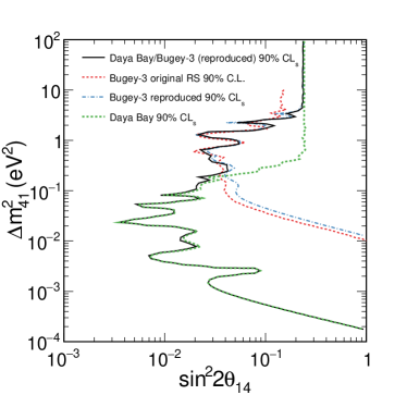
Figure 17: Excluded regions for the combined Daya Bay and reproduced Bugey-3 results [187]. The region to the right of the curve is excluded at the 90% CL_s. The original Bugey-3 result [24] using a raster scan (RS) [188], the reproduced Bugey-3 result with adjusted fluxes, and Daya Bay result [182] are shown as well.

The Bugey-3 experiment was performed in the early 1990s at the Bugey Nuclear Power Plant located in the Saint-Vulbas commune in France, about 65 km from the Swiss border. The main goal was to search for neutrino oscillation. In this experiment, two LS detectors having a total of three detector modules measured $\bar{\nu}_{e}$ generated from two reactors (reactor 4 and 5) at three different baselines (15 m, 40 m, and 95 m) [24]. Each detector module was a 600-liter ⁶Li-doped LS having dimensions of 122$\times$62$\times$85 cm³ [189]. Each module was optically divided into independent cells having dimensions of $8\times 8\times 85$ cm³. Every cell was instrumented on each side by a PMT. The pressurized water reactor was approximated as a cylinder of $\sim$1.6 m radius and $\sim$3.7 m height. Bugey-3 detected IBD interactions with recoil neutrons captured by ⁶Li (see Table 2). The energy resolution was about 6% at 4.2 MeV. The ratios of the measured positron energy spectrum to the Monte Carlo prediction at all three distances did not show any signature of oscillation, and exclusion contours were made in the phase space of $\sin^{2}2\theta_{14}$ and $\Delta m^{2}_{41}$ (see Fig. 17).

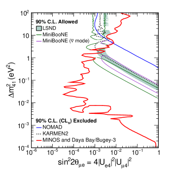
Figure 18: MINOS and Daya Bay/Bugey-3 combined 90% CL_s limit on $\sin^{2}2\theta_{\mu e}$ [187] are compared to the LSND and MiniBooNE 90% C.L. allowed regions. Regions of parameter space to the right of the red contour are excluded. The regions excluded at 90% C.L. by KARMEN2 [190] and NOMAD [191] are also shown.

The main motivation of the Daya Bay experiment (described in Sec. 3.3) was to perform precision measurements of $\sin^{2}2\theta_{13}$ and $\Delta m^{2}_{ee}$. Given its unique configuration of multiple baselines to three groups of nuclear reactors, the Daya Bay experiment also allowed a search for sterile neutrinos through relative spectral distortions obtained at three experimental sites. With a baseline longer than that of Bugey-3, Daya Bay was sensitive to the sterile neutrino mixing parameter $\sin^{2}2\theta_{14}$ at smaller $\Delta m^{2}_{41}$ values.

Similar to that of Bugey-3, no oscillation signature attributable to an additional sterile neutrino was found, and exclusion contours were set in Refs. [181, 182] using the Feldman–Cousins [192] and CL_s [193, 194] approaches. Figure 17 shows the combined results of Daya Bay and Bugey-3 [187] using the Gaussian CL_s method [195]. The exclusion contour combining both experiments covered about 5 orders of magnitude in $\Delta m^{2}_{41}$. This result was further combined with results from the MINOS experiment [196] to constrain the anomalous (anti-)$\nu_{\mu}\rightarrow$(anti-)$\nu_{e}$ oscillation [187] using the CL_s method [193, 194, 197]. As shown in Fig. 18, the combined result from Daya Bay, Bugey-3, and MINOS excluded most of regions allowed by LSND and MiniBooNE. Together with the search results from the IceCube experiment using the matter effect [198], this result significantly reduced the allowed parameter space for future searches.

The NEOS [183] experiment searched for a light sterile neutrino at reactor unit 5 (2.8-GW thermal power) located at the Hanbit nuclear power complex in Yeonggwang, South Korea, which is the same reactor complex used by the RENO experiment [138]. The active core size was 3.1 m in diameter and 3.8 m in height. In this experiment, the search was performed with 1 ton of 0.5% Gd-loaded LS at a distance of about 24 m from the reactor core. The LS was contained in a horizontal cylindrical stainless-steel tank of 103 cm in diameter and 121 cm in length. Each end of the target vessel was exposed to 19 8-inch PMTs that were packed inside mineral oil. The energy response of the NEOS detectors was calibrated with various radioactive sources. The energy resolution was measured to be about 5% at 1 MeV. With 20-m m.w.e. overburden and active muon veto counters made from 5-cm thick plastic scintillators surrounding the detector, NEOS achieved a 22:1 signal-to-background ratio after all cuts.

With a single detector, NEOS relied on external constraints on the neutrino spectrum to search for spectral distortion. In comparison with the neutrino spectrum measured from the Daya Bay experiment [199], NEOS observed no significant spectral distortion caused by oscillation, and the exclusion limit was set using the raster-scan method [188]. As shown in Fig. 19, stringent exclusion limits were set in the mass range of $0.2$ eV² $<\Delta m^{2}_{41}<$ 3 eV².

Table 6: Major parameters of very–short–baseline reactor neutrino experiments that are in operation, under construction, or being planned. Diameter, radius, and height are indicated by d, r, and h, respectively. For the energy resolution, the unit of the energy ‘E’ is MeV. For signal-to-background ratios, the achieved performances (A.) are separated from the expected performance (E.). ‘Seg.’ stands for segmentation.

Experiment	Reactor	Distance	Mass	Resolution	Seg.	S/B
DANSS	LEU 3.1 GWth	10.7-12.7 m	1.1 Ton	17%/$\sqrt{E}$	2D	0.6 (A.)
Ref. [184, 200]	1.5 m r $\times$ 3.5 m h
NEOS	LEU 2.8 GW	24 m	1 Ton	5%/$\sqrt{E}$	1D	21 (A.)
Ref. [183]	3.1 m d $\times$ 3.8 m h
NEUTRINO-4	HEU 100 MW	6-12 m	0.3 Ton	N/A	2D	0.25-0.3 (A.)
Ref. [201, 202]	0.35$\times$0.42$\times$0.42 m3
Nucifer	HEU 70 MW	7.2 m	0.6 Ton	10%/$\sqrt{E}$	1D	0.06 (A.)
Ref. [203, 204]	0.3 m r$\times$ 0.6 m h
PROSPECT	HEU 85 MW	7-12 m	1.5 Ton	4.5%/$\sqrt{E}$	2D	0.8 (A.)
Ref. [38, 205]	0.2 m r $\times$0.5 m h
STEREO	HEU 58 MW	8.9-11.1 m	1.6 Ton	8%/$\sqrt{E}$	2D	0.9 (A.)
Ref. [206, 207]	0.4 m d $\times$ 0.8 m h
SOLID	HEU 75 MW	6-9 m	1.6 Ton	14%/$\sqrt{E}$	3D	1.0 (E.)
Ref. [208, 209]	0.25 m r
NuLAT	HEU 20 MW	4 m	1 Ton	4%/$\sqrt{E}$	3D	3 (E.)
Ref. [210]	1 m d
CHANDLER	HEU 75 MW	5.5-10 m	1 Ton	6%/$\sqrt{E}$	3D	3 (E.)
Ref. [211]	0.25 m r

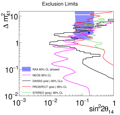
Figure 19: Exclusion limits reported at the Neutrino 2018 conference [92] from the new generation of very–short–baseline reactor neutrino experiments. The results from DANSS [184] (90% CL_s), PROSPECT [185] (95% CL), and STEREO [186] (90% CL) are preliminary. The allowed region from the reactor antineutrino anomaly (RAA) is compared. The star represents the best-fit point.

A new generation of very–short–baseline reactor neutrino experiments to search for an eV-mass-scale sterile neutrino are under construction or in operation. Table 6 summarizes the major parameters of these experiments. The primary challenges for these experiments include the cosmogenic backgrounds resulting from the limited amount of overburden, and reactor-related backgrounds caused by the proximity of the detector to the reactor core. A segmented detector design is generally required to achieve a desired signal-to-noise ratio.

The sensitivity of a light sterile neutrino typically depends on the distance between the detector and the reactor core, statistics (target mass, reactor power, and signal to noise ratio), sizes of reactor core and detector (smearing in distance), and energy resolution (smearing in energy). A comparison of measurements at different distances is crucial for finding evidence of a sterile neutrino. At the Neutrino 2018 conference [92], three of these experiments: DANSS [184], PROSPECT [185], and STEREO [186], reported preliminary exclusion limits shown in Fig. 19.

The DANSS experiment is located at the Kalinin nuclear power plant in Russia. The detector was placed in a room below the reactor with an overburden of $\sim$50 m.w.e. Polystyrene-based plastic scintillator strips (1 cm$\times$4 cm$\times$1 m) with a thin Gd-containing coating were arranged with two orientations in different layers. A total of 2500 strips were coupled to 2500 silicon photomultipliers and 50 PMTs [200]. Data were taken at three vertical detector positions with baseline varying from 10.7 m to 12.7 m. With about 1 million IBD events after background subtraction, DANSS observed no significant spectral distortion when comparing the positron energy spectrum measured at different detector positions [184]. As shown in Fig. 19, DANSS excluded the best-fit point of the RAA with a confidence level higher than 5$\sigma$.

The PROSPECT experiment is located at the 85-MW high flux isotope reactor (HFIR) at Oak Ridge National Laboratory in the United States. With a compact reactor core and short baselines (7 m – 9 m), PROSPECT had good sensitivities for $\Delta m^{2}_{41}$ above 3 eV². The detector consisted of 154 segments (119 cm$\times$15 cm$\times$15 cm) filled with ⁶Li-doped EJ-309 LS. Each segment was read from two PMTs at each end. The ⁶Li-doped LS allowed a good pulse shape discrimination for the delayed signal [212], which was essential for rejecting cosmogenic and reactor-related backgrounds. Using multiple layers of shielding, PROSPECT achieved an overall signal to background ratio ($\sim$0.8). With a total 25k IBD events after background subtraction, energy spectra from six baselines were compared. No oscillation signal was observed [185] and exclusion limits were set. As shown in Fig. 19, the best-fit point of the RAA was excluded by PROSPECT with a confidence level of 2.2$\sigma$.

The STEREO experiment is located at a 58-MW research reactor at Institut Laue–Langevin (ILL) in Grenoble, France. Similar to PROSPECT, the research reactor core is compact and the baseline ranges from 9 m to 11 m. The target (dimensions 2.2 m$\times$0.9 m$\times$1.2 m) was longitudinally divided into six identical and optically separated cells filled with Gd-loaded LS. With about 15 m.w.e. overburden, the STEREO detector was further shielded by a combination of lead, polythylene, and boron-loaded rubber. A water Cerenkov muon veto was installed on top of the detector. About 400 IBD events were detected per day when reactor was on and a signal to background ratio of 0.9 was achieved [207]. With 66 (138) days of reactor on (off) data, no oscillation signal was observed when the measured spectra from six cells were compared [186]. As shown in Fig. 19, the best-fit point of the RAA was excluded by STEREO with a confidence level of 97.5%.

In the next few years, more precise results are expected from the new generation of very–short–baseline reactor neutrino experiments. Together with searches for a light sterile neutrino with atmospheric neutrinos [198], accelerator neutrinos [213], pion/kaon decay-at-rest (DAR) neutrinos, and radioactive neutrino sources [214], these reactor neutrino experiments are expected to give a definitive answer regarding the existence of a eV-mass-scale light sterile neutrino.

4.3 Reactor Antineutrino Anomaly

The reactor antineutrino anomaly [177] refers to a deficit of the measured antineutrino rate in short-baseline reactor experiments ($L<2$ km) with respect to the latest calculations of the antineutrino flux [46, 47], which are about 5% higher than previous calculations [56, 57, 58, 52]. The initial calculation of this deficit in Ref. [177] is biased towards a larger value by about 1.5% [215] because of an improper treatment of flux uncertainties in the covariance matrix, as demonstrated in Ref. [216]. Figure 20 displays the updated global fit, showing a data-over-prediction ratio of $0.943\pm 0.008$, excluding uncertainties associated with the flux prediction.

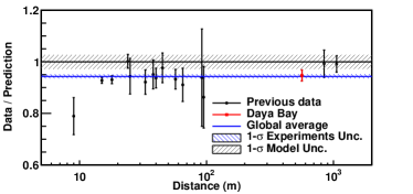
Figure 20: The measured reactor $\bar{\nu}_{e}$ rate as a function of the distance from the reactor, normalized to the theoretical prediction of the Huber–Mueller model [47, 217], taken from Ref. [199]. The rate is corrected for three-flavor neutrino oscillation at each baseline. The blue shaded region represents the global average and its 1$\sigma$ uncertainty. The 2.7%-model uncertainty is shown as a band around unity. Measurements at the same baseline are combined for clarity. The Daya Bay measurement is shown at the flux-weighted baseline (573 m) of the two near halls.

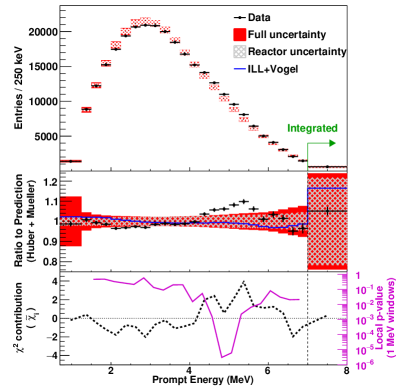
Figure 21: Predicted and measured prompt-energy spectra, taken from Ref. [199]. The prediction is based on the Huber–Mueller model [47, 217] and normalized to the number of measured events. The highest energy bin contains all events above 7 MeV. The gray hatched and red filled bands represent the square-root of diagonal elements of the covariance matrix for the reactor-related and the full (reactor, detector, and background) systematic uncertainties, respectively. The error bars on the data points represent the statistical uncertainty. The ratio of the measured prompt-energy spectrum to the predicted spectrum (Huber–Mueller model) is shown in the middle panel. The blue curve shows the ratio of the prediction based on the ILL+Vogel [52, 56, 57, 58] model to that based on the Huber–Mueller model. The defined $\chi^{2}$ distribution of each bin (black dashed curve) and local p-values for 1-MeV energy windows (magenta solid curve) are shown in the bottom panel.

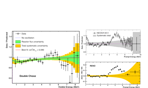
Figure 22: Observations of the 5-MeV prompt energy excess with respect to the model prediction [46, 47] from RENO [138], Double Chooz [142], and NEOS [183].

The calculated deficit cannot be explained by the quoted uncertainties of the reactor flux model [46, 47], which is around 2%. One potential explanation of this deficit is the existence of a sterile neutrino with its corresponding mass eigenstate heavier than or equal to $\sim$1 eV. Recently, the foundation of this explanation was challenged by authors of Ref. [61], who carefully examined the flux spectrum calculation and concluded that the uncertainties of the flux calculation should be larger than 5%. Their conclusion was supported by the recent measurements of the reactor neutrino energy spectrum from the Daya Bay [199], RENO [138], Double Chooz [142], and NEOS [183] experiments. Figure 21 shows the measured prompt energy spectrum from Daya Bay [199] in comparison with the model prediction and its associated uncertainties.

An excess between the 4 MeV and 6 MeV prompt energy beyond the model uncertainties can be clearly seen, which indicates an underestimation of the model uncertainties. Taking into account the entire energy range, this result disfavors the model prediction [46, 47] at about 2.6$\sigma$. For the 2-MeV window between 4 MeV and 6 MeV, the p-value in testing the compatibility between the measurement and calculation reaches 5$\times 10^{-5}$, corresponding to a 4.0$\sigma$ deviation.

Such an excess having a similar degree of deviation was also observed when compared with the ILL+Vogel [52, 56, 57, 58] model calculation. Figure 22 compiles the observations of this excess from recent reactor neutrino experiments: RENO [138], Double Chooz [142], and NEOS [183]. In addition, a re-analysis of positron spectrum from the Gösgen experiment, which was performed with a nuclear power plant at Switzerland in the 1980’s [22], also revealed a similar excess [218]. The observation of this 5-MeV prompt energy excess has motivated many studies attempting to explain its origin (See  [217, 219, 220, 221], among others). At the moment, the exact origin of the 5-MeV prompt energy excess is still not clear. Nevertheless, it indicates that the original 2% quoted model uncertainty was underestimated.

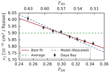
Figure 23: Measurements of IBD yield per fission, $\sigma_{f}$ (black), versus effective ²³⁹Pu (lower axis) or ²³⁵U (upper axis) fission fractions, taken from Ref. [222]. The predicted yields from the Huber–Mueller model [46, 47] (blue), scaled to account for the difference in total yield between data and prediction, are shown. A clear discrepancy is seen between measurements and model predictions.

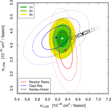
Figure 24: Allowed regions (filled colored contours) in the $\sigma_{f,235}$-$\sigma_{f,239}$ plane obtained from the combined fit of the reactor rates [223] and the Daya Bay measurement of $\sigma_{f,235}$ and $\sigma_{f,239}$ [222], taken from Ref. [224]. The red, blue and black curves enclose, respectively, the allowed regions obtained from the fit of the reactor rates [223], the allowed regions corresponding to the Daya Bay measurement [222], and the theoretical Huber–Mueller model [46, 47] allowed regions.

In addition to the measured reactor neutrino energy spectra, evidence also indicates the underestimation of the model uncertainties from the extracted antineutrino flux of ²³⁵U and ²³⁹Pu. Figure 23 shows the measured IBD yield per fission, $\sigma_{f}$, as a function of the effective ²³⁹Pu fission fraction from Daya Bay [222]. The data from Daya Bay after an overall normalization correction to account for the rate deficit still deviated from the prediction of the Huber–Mueller model [46, 47]. Taking into account the original model uncertainty as well as the measurement uncertainties, the Huber–Mueller model prediction was disfavored at $\sim$3.1$\sigma$.

These data were further used to extract the IBD yield per ²³⁵U fission, $\sigma_{235}$, and the IBD yield per ²³⁹Pu fission, $\sigma_{239}$. The IBD yield per ²⁴¹Pu (²³⁸U) fission, $\sigma_{241}$ ($\sigma_{238}$), which contributes about 5% (10%) to the antineutrino flux, was conservatively constrained to 10% uncertainty.

The 2D confidence interval for $\sigma_{235}$ vs. $\sigma_{239}$ from Daya Bay is shown in Fig. 24. In comparison, the results from Ref. [224] are shown after analyzing the measured rates from all the short-baseline reactor experiments with various average fission fractions. In the latter analysis, the uncertainties of $\sigma_{238}$ and $\sigma_{241}$ were conservatively taken to be 15% and 10%, respectively.

In comparison, with the predictions from the Huber–Mueller model [46, 47], both results showed a clear deficit in $\sigma_{235}$. The uncertainty of $\sigma_{235}$ from the rate analysis was smaller than that of the Daya Bay fuel-evolution analysis, as some of the short-baseline experiments were performed with highly-enriched ²³⁵U. In contrast, the uncertainty of $\sigma_{239}$ from the Daya Bay fuel-evolution analysis was smaller than that of the rate analysis. Within experimental uncertainties, both measurements of $\sigma_{239}$ were consistent with that from Huber–Mueller model.

In summary, the analysis of measured reactor neutrino energy spectra and fuel evolution from Daya Bay suggests an underestimation of the calculated reactor neutrino flux, which has shaken the foundation of the light-sterile-neutrino explanation of the reactor antineutrino anomaly. On the other hand, an increase of the reactor neutrino flux uncertainties also enlarges the allowed phase space for sterile neutrino couplings (i.e., $\sin^{2}2\theta_{14}$ and $\Delta m^{2}_{41}$). Additional measurements are thus necessary to fully address this question.

5 Additional Physics Topics Using Reactor Neutrinos

The high statistics data acquired by reactor neutrino experiments, together with the accurate determination of the antineutrino energy using the IBD reaction, have prompted various searches for new effects within or beyond the paradigm of three-flavor neutrino oscillation. The search for a light sterile neutrino, discussed in the previous section, is a prime example. In this section, we discuss examples of other searches for new effects, including the search for the neutrino magnetic moment, the attempt to constrain characteristics of the wave-packet approach for neutrino oscillation, the test of the Leggett–Garg inequality, and the search for the breaking of Lorentz and CPT invariance.

5.1 Search for the Neutrino Magnetic Moment via Neutrino-electron Scattering

A natural extension to the standard model is the potential existence of neutrino electromagnetic interactions with virtual photons [225, 226, 227], which can be described at low-momentum transfer by two phenomenological parameters, the anomalous magnetic moment $\mu_{\nu}$ and the mean-square charge radius $\langle r^{2}\rangle$ [48]. A non-zero $\mu_{\nu}$ would enable left-handed neutrinos to flip into sterile right-handed neutrinos in a magnetic field. In the minimal standard model, neutrinos are massless and have no magnetic moment. A non-zero moment can be generated through radiative corrections [228, 229] for massive Dirac neutrinos in a simple extension [230]:

$$\mu_{\nu}=\frac{3G_{F}m_{e}m_{\nu}}{4\sqrt{2}\pi^{2}}=3.2\times 10^{-19}\left(\frac{m_{\nu}}{1~{}eV}\right)\cdot\mu_{B},$$ (45)

with $m$ representing the mass and $\mu_{B}\equiv e/2m_{e}$ being the electron Bohr magnetons. In comparison, $\langle r^{2}\rangle$ conserves helicity in interactions between a neutrino and a charged particle. The interpretation of $\langle r^{2}\rangle$ is still under debate. On one hand, authors of Refs. [228, 231, 232] showed that a straightforward definition of $\langle r^{2}\rangle$ was gauge-dependent and thus unphysical. On the other hand, authors of Refs. [233, 234, 235] interpreted $\langle r^{2}\rangle$ as a physical observable, and $\langle r_{\bar{\nu}_{e}}^{2}\rangle=0.4\times 10^{-32}$ cm² was predicted within the standard model framework.

For reactor neutrinos, both $\mu_{\nu}$ and $\langle r^{2}\rangle$ can be accessed through the neutrino-electron elastic scattering having a cross section [48]:

$$\frac{d\sigma}{dT}=\frac{G_{F}^{2}m_{e}}{2\pi}((g_{V}+x+g_{A})^{2}$$

$$+(g_{V}+x-g_{A})^{2}\left(1-\frac{T}{E_{\nu}}\right)^{2})+(g^{2}_{A}-(g_{V}+x)^{2})\frac{m_{e}T}{E_{\nu}^{2}})$$

$$+\frac{\pi\alpha^{2}\mu_{\nu}^{2}}{m_{e}^{2}}\frac{1-T/E_{\nu}}{T},$$ (46)

where $E_{\nu}$ is the neutrino energy and

$$g_{V} = 2\sin^{2}\theta_{W}+1/2$$

$$g_{A} = -1/2$$

$$x = \frac{\sqrt{2}\pi\alpha}{3G_{F}}\langle r^{2}\rangle$$ (47)

for $\bar{\nu}_{e}$. Here, $\theta_{W}$ is the weak mixing angle and $T$ stands for the kinetic energy of the scattered electron. In particular, the $1/T$ term associated with $\mu_{\nu}$ leads to a significant increase of the cross section at low kinetic energies. Therefore, the most sensitive direct limit, $\mu_{\nu}<3.2\times 10^{-11}\mu_{B}$, came from high-purity germanium detectors at about a 10-keV threshold [236, 237, 238]. The $\mu_{\nu}$ contribution at the present limit are still orders of magnitude higher than the standard model prediction. Other technologies, such as time projection chamber [67], organic scintillator [65], and scintillating crystal [49], were also used to set direct limits on $\mu_{\nu}$. A relaxed indirect limit on $\mu_{\nu}$ was set by KamLAND’s search for solar $\bar{\nu}_{e}$ [239]. In addition, limits on $\langle r_{\bar{\nu}_{e}}^{2}\rangle$ were set at a few times $10^{-32}$ cm² [49, 65]. Neutrino-electron elastic scattering from reactor neutrinos can also be used to perform (precision) measurements of the weak mixing angle $\theta_{W}$ at low momentum transfer [64, 49].

5.2 Wave Packet and Neutrino Oscillation

The phenomenon of neutrino oscillation is usually formulated as a quantum mechanical effect using a plane-wave approximation. While successful in describing many neutrino oscillation results, the plane-wave approach can lead to apparent paradoxes [240, 241]. The necessity of a wave-packet treatment for neutrino oscillation has been considered since the 1970s [242, 243]. The wave-packet models of neutrino oscillation contain a quantity $\sigma_{p}$ that effectively describes the momentum dispersions of all particles involved in the production and detection of neutrinos. A consequence of a non-zero value of $\sigma_{p}$ is the ‘decoherence’  of the quantum superposition of mass eigenstates, leading to a modification or diminishing of the neutrino oscillation pattern. Moreover, the width of the wave packet would also broaden as time elapses, as a result of the momentum dispersion.

Despite many theoretical advances in formulating the wave packet models, within quantum mechanical or field-theoretical approaches, no quantitative estimates for $\sigma_{p}$ or the related spatial width $\sigma_{x}=\left(2\sigma_{p}\right)^{-1}$ are available. A treatment of the decoherence length for neutrinos produced in pion decays using density matrix formalism was recently performed [244]. For antineutrinos produced in reactors, estimates for $\sigma_{x}$ vary from $\sim$10^-12 cm (the size of the uranium nucleus) to $\sim 10^{-7}$ cm (atomic scale), corresponding to $\sigma_{p}\sim$10 MeV to $\sigma_{p}\sim$100 eV [245].

The recent high-statistics reactor neutrino oscillation data have provided an opportunity to compare these data against the wave-packet approach and to set a constraint on the momentum dispersion of the wave packet for the first time [245]. In particular, a search for possible decoherence effects in neutrino oscillation was performed using Daya Bay data. The good energy resolution, together with large statistics collected at multiple baselines, allowed a meaningful study of quantum decoherence effects based on these data.

In the wave-packet approach, the probability of a neutrino’s oscillating from flavor $\alpha$ to $\beta$ at a distance $L$, $P_{\alpha\beta}(L)$, can be written as [245]

$$P_{\alpha\beta}=\sum_{k,\,j=1}^{3}\frac{V^{*}_{\alpha k}V^{\phantom{*}}_{\beta k}V^{\phantom{\dagger}}_{\alpha j}V^{*}_{\beta j}}{\sqrt[4]{1+\left(L/L^{\mathrm{d}}_{kj}\right)^{2}}}\mathrm{e}^{-\frac{\left(L/L^{\mathrm{coh}}_{kj}\right)^{2}}{1+\left(L/L^{\mathrm{d}}_{kj}\right)^{2}}-\mathrm{D}^{2}_{kj}-i\widetilde{\varphi}_{kj}},$$ (48)

where $V_{\alpha k}$ is the usual neutrino mixing matrix element. Three length scales appear in Eq. (48):

$$L^{\mathrm{osc}}_{kj}=\frac{4\pi p}{\Delta m^{2}_{kj}},~{}~{}L^{\mathrm{coh}}_{kj}=\frac{L^{\mathrm{osc}}_{kj}}{\sqrt{2}\pi\sigma_{\mathrm{rel}}},~{}~{}L^{\mathrm{d}}_{kj}=\frac{L^{\mathrm{coh}}_{kj}}{2\sqrt{2}\sigma_{\mathrm{rel}}},$$ (49)

where the relative momentum spread, $\sigma_{\mathrm{rel}}=\sigma_{p}/p$, is a Lorentz invariant quantity. $L^{\mathrm{osc}}_{kj}$ refers to the usual oscillation length where maximal oscillation occurs for the neutrino mass-squared difference $\Delta m^{2}_{kj}$. The neutrino coherence length, $L^{\mathrm{coh}}$, corresponds to the distance at which the wave packet splits into non-overlapping components, diminishing the interference between neutrino mass eigenstates $k$ and $j$. The dispersion length, $L^{\mathrm{d}}$, characterizes the distance when the spatial widths of the wave packets for $k$ and $j$ mass eigenstates differ sufficiently because of momentum dispersion, and oscillation is suppressed. The quantity $\mathrm{D}_{kj}$ in Eq. (48) is given as

$$\mathrm{D}_{kj}=\frac{\sqrt{2}\pi\sigma_{x}}{L_{kj}^{\mathrm{osc}}},$$ (50)

which suppresses the oscillation when the spatial width, $\sigma_{x}$, of the wave packet is large compared with the oscillation width, $L^{\mathrm{osc}}_{kj}$. The expression for the phase $\widetilde{\varphi}_{kj}$, which is the sum of the usual plane-wave phase $\varphi_{kj}=2\pi L/L^{\mathrm{osc}}_{kj}$ and another correction term arising from the wave packet, can be found in Ref. [245].

From Eq. (48) and Eq. (50), in the limits of $\sigma_{p}\to 0$ or $\sigma_{p}\to\infty$, the oscillation probability in Eq. (48) becomes

$$P_{\alpha\beta}=\sum_{k}|V_{\alpha k}|^{2}|V_{\beta k}|^{2}.$$ (51)

The interference terms with $k\neq j$ in Eq. (48) now all vanish. Thus $P_{\alpha\beta}$ is now independent of distance, and the oscillation pattern disappears. This result can be understood intuitively. As $\sigma_{p}\to 0$, the spatial width of the wave packet approaches infinity, washing out any oscillation pattern having a finite oscillation length. Similarly, an infinite $\sigma_{p}$ gives zero coherence and dispersion lengths, preventing any interference effects. Observation of oscillation behavior in reactor neutrino experiments clearly shows that $\sigma_{p}$ must lie somewhere between these two extremes.

The Daya Bay Collaboration has performed [245] a fit to the neutrino oscillation data utilizing the wave packet oscillation expression of Eq. (48). The allowed region for $\sigma_{\mathrm{rel}}$ at a 95% C.L. was found to be $2.38\times 10^{-17}<\sigma_{\mathrm{rel}}<0.23$. Adding the constraints of the sizes of the reactor cores and detectors, the upper limit reduces to 0.20, corresponding to $10^{-11}\mathrm{cm}\lesssim\sigma_{x}\lesssim 2$ m. It is worth noting that the lower limit in $\sigma_{x}$ is roughly 10 times the size of the uranium nucleus.

With additional data from Daya Bay, the sensitivity on the upper limit of $\sigma_{\mathrm{rel}}$ is expected to be improved by $\sim$30%. Nevertheless, a decoherence effect from the wave-packet approach was found to be insignificant for the Daya Bay experiment [245]. Thus, the neutrino oscillation parameters $\sin^{2}2\theta_{13}$ and $\Delta m^{2}_{32}$ extracted from the plane-wave approach are entirely reliable.

5.3 Leggett–Garg Inequality and Neutrino Oscillation

The phenomenon of neutrino oscillation is fundamentally a quantum mechanical effect. It originates from the principle of superposition, which allows a neutrino flavor eigenstate to be expressed as a coherent superposition of neutrino mass eigenstates. As discussed in Sec. 5.2, decoherence effects would lead to the disappearance of neutrino oscillation.

The superposition principle remains an enigmatic and nonintuitive ingredient of the quantum mechanics. At the macroscopic level, a system’s being able to coexist in different states led to the famous paradox of Schrödinger’s cat [246]. At the microscopic level, the celebrated Bell’s inequality [247] was proposed as a quantitative means to probe quantum mechanical coherence, or entanglement, within a spatially separated system. While Bell’s inequality has been extensively tested, a loophole-free test of this inequality remains an elusive goal.

In 1985, Leggett and Garg [248] proposed a new test of quantum coherence not only for microscopic systems, for which Bell’s inequality applies, but also for macroscopic systems. To facilitate such a test for macroscopic systems, Leggett and Garg considered the correlations of a single system measured at different times.

The Leggett–Garg inequality (LGI) is derived based on two principles: macroscopic realism (MR) and non-invasive measurability (NIM). Realism, often encoded in hidden-variable theories, implies that a measurement on a system reveals a pre-existing value. Under realism, systems prepared identically can be distinguished via a set of hidden variables, and a measurement would uncover a pre-existing value. NIM stipulates that a measurement could be performed without disturbing the system. While MR and NIM are consistent with classical mechanics, they certainly contradict quantum mechanics. The LGI provides a method to test the applicability of quantum mechanics to macroscopic systems, and LGI is often regarded as the time analogue of Bell’s inequality [249]. A recent review on LGI can be found in Ref. [250].

The LGI involves the two-time correlation function $C_{ij}=\langle Q(t_{i})Q(t_{j})\rangle$, where $Q$ is a dichotomic observable with $Q=\pm 1$. The value of $C_{ij}$ is obtained by summing over the four possible values of $Q(t_{i})Q(t_{j})$ (namely, +1, -1, -1, +1) weighted by the corresponding probability $P_{ij}(Q_{i},Q_{j})$. From $C_{ij}$ the quantity $K_{n}$ could be defined from measurements performed at $n$ distinct times:

$$K_{n}=C_{21}+C_{32}+C_{43}+\cdot\cdot+C_{n(n-1)}-C_{n1}.$$ (52)

Under the assumptions of MR and NIM, Leggett and Garg obtained the inequality $K_{n}\leq n-2$ for $n\geq 3$.

Twenty-five years after the work of Leggett and Garg, the first observation of the violation of LGI was reported [251], followed by many other LGI tests [250]. However, most of the tests suffer from the ‘clumsiness loophole’ [252], for which the LGI violation could be attributed to unintentional disruption of the system during measurements. This loophole could be avoided by using weak or indirect measurements.

The idea of testing LGI using neutrino oscillation was proposed several years ago [253], and the first test was performed recently [254]. As an example, consider the case of reactor neutrino oscillation with an electron antineutrino at $t=0$. If at time $t$, a measurement finds an electron antineutrino, then $Q=+1$. Otherwise, $Q=-1$. The key idea is to mimic a series of measurements at various times on a single neutrino by measurements made on an ensemble of neutrinos of various energies at a given time. Details of this method can be found in Refs. [253, 254]. One unique feature of this method is the long coherence length for neutrino oscillation, unlike other LGI tests involving much shorter coherence lengths. This method is also free from the ‘clumsiness loophole’. Using the MINOS muon neutrino oscillation data at a baseline of 735 km, the LGI for $K_{3}$ and $K_{4}$ was found to be violated at a level greater than $6\sigma$ [254]. A recent analysis of the Daya Bay data also showed a very similar result [255].

5.4 Lorentz Violation and Neutrino Oscillation

The standard model and general relativity (GR) are believed to be the low-energy limit of a theory that unifies quantum physics and gravity at the Planck scale, $M_{P}\approx 10^{19}$ GeV. An effective field theory at lower energies, called the standard-model extension (SME) [256, 257, 258], extends the GR-coupled SM by including Lorentz-violating terms constructed from SM and GR fields. The Lorentz and CPT violations in the SME are caused by background Lorentz tensor fields of the Universe. These background fields are fixed in spacetime, implying rotation and boost dependence of physics in a specific frame. While suppressed at presently accessible energy $E$ by an order of $\sim$E/M_P, the predicted violations of Lorentz and CPT symmetries might be revealed in sensitive measurements.

Quantum interference phenomena such as neutral-meson oscillation [259] and neutrino oscillation [260] might provide sensitive searches for the Lorentz and CPT violations predicted by the SME. A small coupling between neutrinos and a Lorentz-violating field can conceivably alter the pattern of neutrino oscillation [260]. In the SME, the effective Hamiltonian for neutrino oscillation is given as [260]

$$(h^{\nu}_{eff})_{ab}\sim\frac{(m^{2})_{ab}}{2E}+\frac{1}{E}[(a_{L})^{\mu}p_{\mu}-(c_{L})^{\mu\nu}p_{\mu}p_{\nu}]_{ab},$$ (53)

where $a$ and $b$ refer to the neutrino flavors and $E$ and $p_{\mu}$ are the energy and the energy-momentum 4-vector of the neutrino, respectively. The first term on the right-hand-side of Eq. (53) is the SM contribution from massive neutrinos. The coefficients $(a_{L})^{\mu}_{ab}$ have dimensions of mass and violate both Lorentz and CPT symmetry, while the dimensionless coefficients $(c_{L})^{\mu\nu}_{ab}$ violate Lorentz but keep CPT symmetry. The CPT-odd $(a_{L})^{\mu}_{ab}$ changes sign for antineutrinos and can lead to differences between neutrino and antineutrino oscillation.

This CPT-violating feature of SME offered an attractive possible explanation [261] for the LSND $\nu_{\mu}\to\nu_{e}$ result [173]. Moreover, the vector $(a_{L})^{\mu}_{ab}$ and tensor $(c_{L})^{\mu\nu}_{ab}$ coefficients introduce directional dependence of neutrino oscillation. If the $Z$-axis is chosen as the rotation axis of the Earth, then a sidereal variation of the neutrino direction in $X$ and $Y$ would occur. Therefore, a sidereal variation of neutrino oscillation can be caused by coefficients $(a_{L})^{\mu}_{ab}$, $(c_{L})^{\mu\nu}_{ab}$, for which at least one of $\mu$ and $\nu$ is either $X$ or $Y$. In other words, all coefficients except $(a_{L})^{T}_{ab}$, $(a_{L})^{Z}_{ab}$, $(c_{L})^{TT}_{ab}$, $(c_{L})^{TZ}_{ab}$, and $(c_{L})^{ZZ}_{ab}$ can contribute to sidereal variations.

Under SME, the probability for an electron antineutrino $\bar{\nu}_{e}$ to oscillate to $\bar{\nu}_{x}$, where $x$ is $\mu$ or $\tau$, is given as [262]

$$P_{\bar{\nu}_{e}\to\bar{\nu}_{x}} \simeq L^{2}[(C)_{\bar{e}\bar{x}}+(A_{s})_{\bar{e}\bar{x}}\sin(\omega_{\oplus}T_{\oplus})$$ (54)

$$+ (A_{c})_{\bar{e}\bar{x}}\cos(\omega_{\oplus}T_{\oplus})+(B_{s})_{\bar{e}\bar{x}}\sin(2\omega_{\oplus}T_{\oplus})$$

$$+ (B_{c})_{\bar{e}\bar{x}}\cos(2\omega_{\oplus}T_{\oplus})]^{2},$$

where $\omega_{\oplus}$ and $T_{\oplus}$ are the sidereal frequency and sidereal time, and $L$ is the baseline. The expressions for the parameters $A_{s,c}$, $B_{s,c}$, and $C$ consist of the Lorentz-violating coefficients introduced in Eq. (53). Expressions analogous to Eq. (54) can be obtained for oscillations involving other neutrino flavors. For reactor neutrino disappearance experiments, the probability $P_{\bar{\nu}_{e}\to\bar{\nu}_{e}}$ is simply $P_{\bar{\nu}_{e}\to\bar{\nu}_{e}}=1-P_{\bar{\nu}_{e}\to\bar{\nu}_{\mu}}-P_{\bar{\nu}_{e}\to\bar{\nu}_{\tau}}$.

Searches for Lorentz violations in neutrino oscillation via measurements of sidereal modulations of oscillation probability have been performed in accelerator based experiments, including LSND [263], MINOS [264, 265, 266], and MiniBooNE [267], as well as the non-accelerator experiment IceCube [268]. No evidence for Lorentz violating sidereal modulations has been found, setting upper limits on various coefficients in Eq. (53). Combining the analysis of MINOS near-detector (ND) data on $\nu_{\mu}$ and $\bar{\nu}_{\mu}$ disappearance and far-detector (FD) data on $\nu_{\mu}$ disappearance, limits on both the real and imaginary parts of 18 Lorentz-violating coefficients have been obtained [266]. Effects of the $a_{L}$-type ($c_{L}$-type) coefficients are proportional to $L^{2}$ and $(E_{\nu}L)^{2}$, accounting for the greater sensitivities of the FD data [265] for constraining some coefficients, despite its lower event rates compared with the ND data [264]. This consideration also favors the IceCube experiment, which sets a stringent limit for $(c_{L})_{\mu\tau}^{TX(TY)}$ at $3.7\times 10^{-27}$ [268].

The only search for Lorentz violation in reactor neutrino experiments was performed by the Double Chooz Collaboration [269]. The relatively low antineutrino energies and short baseline may limit the reach of reactor-based neutrino experiments. However, unlike the long-baseline MINOS and IceCube experiments, the reactor $\bar{\nu}_{e}$ disappearance experiments are sensitive to Lorentz-violating coefficients in the $e-\tau$ sector. Using 8249 candidate IBD events collected at the Double Chooz FD, constraints on the upper limits of various combinations of 14 of the SME coefficients in the $e-\tau$ sector have been obtained for the first time [269]. With a much longer baseline and much larger detector volume, the JUNO reactor-neutrino experiment [37] is expected to reach even better sensitivities in the search for Lorentz-violating effects in the $e-\tau$ sector.

6 Conclusions

In this article, we review the theoretical and experimental physics associated with man-made reactor neutrinos. Since the discovery of reactor-produced neutrinos in the 1950s, knowledge of the production of reactor neutrinos has been significantly improved. The absolute reactor flux and energy spectrum can now be predicted at the 5% and 10% level, respectively. Inverse beta decay, the primary detection channel of reactor neutrinos, is the most well-understood reaction, allowing for an accurate determination of neutrino energy. Benefiting from these important features, reactor neutrinos have played important roles in establishing the current paradigm of three-neutrino flavor mixing.

At an average baseline of 180 km, the KamLAND experiment observed neutrino oscillation in the solar sector and provided an independent constraint in $\theta_{12}$ and an accurate determination of $\Delta m^{2}_{21}$. At shorter baselines of 1$\sim$2 km, the Daya Bay, RENO, and Double Chooz experiments observed neutrino oscillation, establishing a non-zero value for the last unknown mixing angle, $\theta_{13}$. The discovery of a non-zero $\theta_{13}$ has opened a gateway to access two of the remaining unknowns in the neutrino properties: the CP phase $\delta_{CP}$ that may provide a new source for CP violation, and the mass hierarchy that may provide a crucial input to reveal the Dirac or Majorana nature of neutrino.

The future physics program of reactor neutrinos is quite diversified. On one hand, the JUNO experiment will precisely measure neutrino oscillation at a $\sim$55-km baseline with an excellent energy resolution. The simultaneously measured oscillation caused by ($\theta_{12}$, $\Delta m^{2}_{21}$) and ($\theta_{13}$, $\Delta m^{2}_{32}$) will allow a determination of the neutrino mass hierarchy and a precision measurement of these mixing parameters. On the other hand, a new generation of very-short-baseline reactor experiments will search for a light sterile neutrino. These new measurements together with those using other neutrino sources are expected to explore possible new physics beyond the standard model. As we enter the precision era of neutrino physics, reactor neutrinos might yet lead to other unexpected major discoveries.

7 Acknowledgements

We thank Chao Zhang, Petr Vogel, and Laurence Littenberg for their helpful comments on the manuscript and helpful discussions. We thank Wei Tang for his assistance in preparing some figures and Celia Elliott for her careful reading of the manuscript. This work was supported in part by the National Science Foundation, U.S. Department of Energy, Office of Science, Office of High Energy Physics, under contract number DE-SC0012704.

References

- [1] W. Pauli. Dear radioactive ladies and gentlemen. Phys. Today, 31N9:27, 1978.
- [2] E. Fermi. Trends to a Theory of beta Radiation. (In Italian). Nuovo Cim., 11:1–19, 1934. [,535(1934)].
- [3] E. Fermi. An attempt of a theory of beta radiation. 1. Z. Phys., 88:161–177, 1934.
- [4] H. Bethe and R. Peierls. The ’neutrino’. Nature, 133:532, 1934.
- [5] F. Reines. The neutrino: From poltergeist to particle. Rev. Mod. Phys., 68:317–327, 1996.
- [6] F. Reines and C. L. Cowan. Detection of the free neutrino. Phys. Rev., 92:830–831, 1953.
- [7] C.L. Cowan, F. Reines, F.B. Harrison, H.W. Kruse, and A.D. McGuire. Detection of the free neutrino: A Confirmation. Science, 124:103–104, 1956.
- [8] Frederick Reines and Clyde L. Cowan. The neutrino. Nature, 178:446–449, 1956.
- [9] F. Reines and C. L. Cowan. A Proposed experiment to detect the free neutrino. Phys. Rev., 90:492–493, 1953.
- [10] C. L. Cowan, F. Reines, and F. B. Harrison. Upper limit on the neutrino magnetic moment. Phys. Rev., 96:1294, 1954.
- [11] C. L. Cowan and F. Reines. Neutrino magnetic moment upper limit. Phys. Rev., 107:528–530, 1957.
- [12] F. Reines, C. L. Cowan, and M. Goldhaber. Conservation of the number of nucleons. Phys. Rev., 96:1157–1158, 1954.
- [13] Enrico Fermi. Tentativo di una teoria dell’emissione dei raggi beta. Ric. Sci., 4:491–495, 1933.
- [14] C. Patrignani et al. Review of Particle Physics. Chin. Phys., C40(10):100001, 2016.
- [15] B. Pontecorvo. Mesonium and anti-mesonium. Sov.Phys.JETP, 6:429, 1957.
- [16] B. Pontecorvo. Inverse beta processes and nonconservation of lepton charge. Sov. Phys. JETP, 7:172–173, 1958. [Zh. Eksp. Teor. Fiz.34,247(1957)].
- [17] Ziro Maki, Masami Nakagawa, and Shoichi Sakata. Remarks on the unified model of elementary particles. Prog.Theor.Phys., 28:870–880, 1962.
- [18] B. Pontecorvo. Neutrino Experiments and the Problem of Conservation of Leptonic Charge. Sov.Phys.JETP, 26:984–988, 1968.
- [19] V. N. Gribov and B. Pontecorvo. Neutrino astronomy and lepton charge. Phys. Lett., 28B:493, 1969.
- [20] F. Reines, H. W. Sobel, and E. Pasierb. Evidence for Neutrino Instability. Phys. Rev. Lett., 45:1307, 1980.
- [21] J. F. Cavaignac, A. Hoummada, D. H. Koang, B. Vignon, Y. Declais, H. de Kerret, H. Pessard, and J. M. Thenard. Indication for Neutrino Oscillation From a High Statistics Experiment at the Bugey Reactor. Phys. Lett., 148B:387–394, 1984.
- [22] G. Zacek et al. Neutrino Oscillation Experiments at the Gosgen Nuclear Power Reactor. Phys. Rev., D34:2621–2636, 1986.
- [23] A. I. Afonin, S. N. Ketov, V. I. Kopeikin, L. A. Mikaelyan, M. D. Skorokhvatov, and S. V. Tolokonnikov. A Study of the Reaction on a Nuclear Reactor. Sov. Phys. JETP, 67:213–221, 1988. [Zh. Eksp. Teor. Fiz.94N2,1(1988)].
- [24] Y. Declais et al. Search for neutrino oscillations at 15-meters, 40-meters, and 95-meters from a nuclear power reactor at Bugey. Nucl. Phys., B434:503–534, 1995.
- [25] Z. D. Greenwood et al. Results of a two position reactor neutrino oscillation experiment. Phys. Rev., D53:6054–6064, 1996.
- [26] K. Eguchi et al. First results from KamLAND: Evidence for reactor anti-neutrino disappearance. Phys. Rev. Lett., 90:021802, 2003, hep-ex/0212021.
- [27] G. L. Fogli, E. Lisi, A. Marrone, D. Montanino, and A. Palazzo. Getting the most from the statistical analysis of solar neutrino oscillations. Phys. Rev., D66:053010, 2002, hep-ph/0206162.
- [28] K. S. Hirata et al. Experimental study of the atmospheric neutrino flux. Phys. Lett., B205:416, 1988.
- [29] S. Hatakeyama et al. Measurement of the flux and zenith angle distribution of upward through going muons in Kamiokande II + III. Phys. Rev. Lett., 81:2016–2019, 1998, hep-ex/9806038.
- [30] Y. Fukuda et al. Evidence for oscillation of atmospheric neutrinos. Phys. Rev. Lett., 81:1562, 1998, hep-ex/9807003.
- [31] M. Apollonio et al. Limits on neutrino oscillations from the CHOOZ experiment. Phys.Lett., B466:415–430, 1999, hep-ex/9907037.
- [32] M. Apollonio et al. Search for neutrino oscillations on a long baseline at the CHOOZ nuclear power station. Eur.Phys.J., C27:331–374, 2003, hep-ex/0301017.
- [33] F. Boehm, J. Busenitz, B. Cook, G. Gratta, H. Henrikson, et al. Final results from the Palo Verde neutrino oscillation experiment. Phys.Rev., D64:112001, 2001, hep-ex/0107009.
- [34] F. P. An et al. Observation of electron-antineutrino disappearance at Daya Bay. Phys. Rev. Lett., 108:171803, 2012, 1203.1669.
- [35] J. K. Ahn et al. Observation of Reactor Electron Antineutrino Disappearance in the RENO Experiment. Phys. Rev. Lett., 108:191802, 2012, 1204.0626.
- [36] Y. Abe et al. Indication for the disappearance of reactor electron antineutrinos in the Double Chooz experiment. Phys.Rev.Lett., 108:131801, 2012, 1112.6353.
- [37] Fengpeng An et al. Neutrino Physics with JUNO. J. Phys., G43(3):030401, 2016, 1507.05613.
- [38] J. Ashenfelter et al. The PROSPECT Physics Program. J. Phys., G43(11):113001, 2016, 1512.02202.
- [39] Carlo Bemporad, Giorgio Gratta, and Petr Vogel. Reactor based neutrino oscillation experiments. Rev. Mod. Phys., 74:297, 2002, hep-ph/0107277.
- [40] Xin Qian and Wei Wang. Reactor neutrino experiments: and beyond. Mod. Phys. Lett., A29:1430016, 2014, 1405.7217.
- [41] Petr Vogel, Liangjian Wen, and Chao Zhang. Neutrino Oscillation Studies with Reactors. Nature Commun., 6:6935, 2015, 1503.01059.
- [42] T. Lachenmaier. The measurement of the neutrino mixing angle with reactor neutrino experiments. Prog. Part. Nucl. Phys., 83:31–58, 2015.
- [43] E. A. C. Crouch. Fission-product yields from neutrino-induced fission. Atomic Data and Nuclear Data Tables, 19:417, 1977.
- [44] http://www-nds.iaea.org/standards/.
- [45] U.S. Evaluated Nuclear Data Library ENDF/B-VII 1 http://www.nndc.bnl.gov/exfor/endf00.htm 2006.
- [46] Patrick Huber. On the determination of anti-neutrino spectra from nuclear reactors. Phys.Rev., C84:024617, 2011, 1106.0687.
- [47] Th.A. Mueller, D. Lhuillier, M. Fallot, A. Letourneau, S. Cormon, et al. Improved Predictions of Reactor Antineutrino Spectra. Phys.Rev., C83:054615, 2011, 1101.2663.
- [48] P. Vogel and J. Engel. Neutrino Electromagnetic Form-Factors. Phys. Rev., D39:3378, 1989.
- [49] M. Deniz et al. Measurement of Nu(e)-bar -Electron Scattering Cross-Section with a CsI(Tl) Scintillating Crystal Array at the Kuo-Sheng Nuclear Power Reactor. Phys. Rev., D81:072001, 2010, 0911.1597.
- [50] A. C. Hayes and Petr Vogel. Reactor Neutrino Spectra. Ann. Rev. Nucl. Part. Sci., 66:219–244, 2016, 1605.02047.
- [51] B. R. Davis, P. Vogel, F. M. Mann, and R. E. Schenter. REACTOR ANTI-NEUTRINO SPECTRA AND THEIR APPLICATION TO ANTI-NEUTRINO INDUCED REACTIONS. Phys. Rev., C19:2259–2266, 1979.
- [52] P. Vogel, G.K. Schenter, F.M. Mann, and R.E. Schenter. Reactor Anti-neutrino Spectra and Their Application to Anti-neutrino Induced Reactions. 2. Phys.Rev., C24:1543–1553, 1981.
- [53] H. V. Klapdor and J. Metzinger. Antineutrino Spectrum from the Fission Products of Pu-239. Phys. Rev. Lett., 48:127–131, 1982.
- [54] H. V. Klapdor and J. Metzinger. CALCULATION OF THE ANTI-NEUTRINOS SPECTRUM FROM THERMAL FISSION OF U-235. Phys. Lett., B112:22–26, 1982.
- [55] V. I. Kopeikin. Electron and antineutrino spectra from fragments of fission of 239u, 239pu, 241pu induced by thermal neutrons and of fission of 238u induced by fast neutrons. Sov. J. Nucl. Phys., 32:780, 1980.
- [56] F. Von Feilitzsch, A.A. Hahn, and K. Schreckenbach. EXPERIMENTAL BETA SPECTRA FROM PU-239 AND U-235 THERMAL NEUTRON FISSION PRODUCTS AND THEIR CORRELATED ANTI-NEUTRINOS SPECTRA. Phys.Lett., B118:162–166, 1982.
- [57] K. Schreckenbach, G. Colvin, W. Gelletly, and F. Von Feilitzsch. DETERMINATION OF THE ANTI-NEUTRINO SPECTRUM FROM U-235 THERMAL NEUTRON FISSION PRODUCTS UP TO 9.5-MEV. Phys.Lett., B160:325–330, 1985.
- [58] A.A. Hahn, K. Schreckenbach, G. Colvin, B. Krusche, W. Gelletly, et al. Anti-neutrino Spectra From 241Pu and 239Pu Thermal Neutron Fission Products. Phys.Lett., B218:365–368, 1989.
- [59] N. Haag, A. Gutlein, M. Hofmann, L. Oberauer, W. Potzel, K. Schreckenbach, and F. M. Wagner. Experimental Determination of the Antineutrino Spectrum of the Fission Products of 238U. Phys. Rev. Lett., 112(12):122501, 2014, 1312.5601.
- [60] Petr Vogel. Conversion of electron spectrum associated with fission into the antineutrino spectrum. Phys. Rev., C76:025504, 2007, 0708.0556.
- [61] A.C. Hayes, J.L. Friar, G.T. Garvey, and Guy Jungman, G. Jonkmans. Systematic uncertainties in the analysis of the reactor neutrino anomaly. Phys. Rev. Lett., 112:202501, 2014.
- [62] S. P. Riley, Z. D. Greenwood, W. R. Kropp, L. R. Price, F. Reines, H. W. Sobel, Y. Declais, A. Etenko, and M. Skorokhvatov. Neutrino induced deuteron disintegration experiment. Phys. Rev., C59:1780–1789, 1999, hep-ex/9904001.
- [63] Q. R. Ahmad et al. Measurement of the rate of interactions produced by solar neutrinos at the Sudbury Neutrino Observatory. Phys. Rev. Lett., 87:071301, 2001, nucl-ex/0106015.
- [64] F. Reines, H. S. Gurr, and H. W. Sobel. Detection of anti-electron-neutrino e Scattering. Phys. Rev. Lett., 37:315–318, 1976.
- [65] G. S. Vidyakin, V. N. Vyrodov, I. I. Gurevich, Yu. V. Kozlov, V. P. Martemyanov, S. V. Sukhotin, V. G. Tarasenkov, E. V. Turbin, and S. Kh. Khakhimov. Limitations on the magnetic moment and charge radius of the electron-anti-neutrino. JETP Lett., 55:206–210, 1992. [Pisma Zh. Eksp. Teor. Fiz.55,212(1992)].
- [66] A. I. Derbin, A. V. Chernyi, L. A. Popeko, V. N. Muratova, G. A. Shishkina, and S. I. Bakhlanov. Experiment on anti-neutrino scattering by electrons at a reactor of the Rovno nuclear power plant. JETP Lett., 57:768–772, 1993. [Pisma Zh. Eksp. Teor. Fiz.57,755(1993)].
- [67] Z. Daraktchieva et al. Final results on the neutrino magnetic moment from the MUNU experiment. Phys. Lett., B615:153–159, 2005, hep-ex/0502037.
- [68] J. Hosaka et al. Solar neutrino measurements in super-Kamiokande-I. Phys. Rev., D73:112001, 2006, hep-ex/0508053.
- [69] G. Bellini et al. Measurement of the solar 8B neutrino rate with a liquid scintillator target and 3 MeV energy threshold in the Borexino detector. Phys. Rev., D82:033006, 2010, 0808.2868.
- [70] D. Akimov et al. Observation of Coherent Elastic Neutrino-Nucleus Scattering. Science, 2017, 1708.01294.
- [71] P. Vogel and John F. Beacom. Angular distribution of neutron inverse beta decay, anti-neutrino(e) + p —¿ e+ + n. Phys. Rev., D60:053003, 1999, hep-ph/9903554.
- [72] Alessandro Strumia and Francesco Vissani. Precise quasielastic neutrino/nucleon cross-section. Phys. Lett., B564:42–54, 2003, astro-ph/0302055.
- [73] F. P. An et al. New measurement of via neutron capture on hydrogen at Daya Bay. Phys. Rev., D93(7):072011, 2016, 1603.03549.
- [74] Adam Bernstein, Yi-fang Wang, Giorgio Gratta, and Todd West. Nuclear reactor safeguards and monitoring with anti-neutrino detectors. J. Appl. Phys., 91:4672, 2002, nucl-ex/0108001.
- [75] Patrick Huber and Thomas Schwetz. Precision spectroscopy with reactor anti-neutrinos. Phys. Rev., D70:053011, 2004, hep-ph/0407026.
- [76] N. S. Bowden, A. Bernstein, S. Dazeley, R. Svoboda, A. Misner, and T. Palmer. Observation of the Isotopic Evolution of PWR Fuel Using an Antineutrino Detector. J. Appl. Phys., 105:064902, 2009, 0808.0698.
- [77] Eric Christensen, Patrick Huber, Patrick Jaffke, and Thomas E. Shea. Antineutrino Monitoring for Heavy Water Reactors. Phys. Rev. Lett., 113(4):042503, 2014, 1403.7065.
- [78] L. J. Wen J. Cao and Y. F. Wang. Reactor Neutrino Experiments: Present and Future. Ann. Rev. Nucl. Part. Sci., 67:183–211, 2017, 1803.10162.
- [79] Claudio Giganti, Stéphane Lavignac, and Marco Zito. Neutrino oscillations: the rise of the PMNS paradigm. Prog. Part. Nucl. Phys., 98:1–54, 2018, 1710.00715.
- [80] M. Goldhaber, L. Grodzins, and A. W. Sunyar. Helicity of neutrinos. Phys. Rev., 109:1015–1017, Feb 1958.
- [81] S. Schael et al. Precision electroweak measurements on the resonance. Phys. Rept., 427:257–454, 2006, hep-ex/0509008.
- [82] P. A. R. Ade et al. Planck 2015 results. XIII. Cosmological parameters. Astron. Astrophys., 594:A13, 2016, 1502.01589.
- [83] Nicola Cabibbo. Unitary symmetry and leptonic decays. Phys. Rev. Lett., 10:531–533, Jun 1963.
- [84] Makoto Kobayashi and Toshihide Maskawa. CP Violation in the Renormalizable Theory of Weak Interaction. Prog. Theor. Phys., 49:652–657, 1973.
- [85] Olga Mena and Stephen J. Parke. Unified graphical summary of neutrino mixing parameters. Phys. Rev., D69:117301, 2004, hep-ph/0312131.
- [86] Ivan Esteban, M. C. Gonzalez-Garcia, Michele Maltoni, Ivan Martinez-Soler, and Thomas Schwetz. Updated fit to three neutrino mixing: exploring the accelerator-reactor complementarity. JHEP, 01:087, 2017, 1611.01514.
- [87] L. Wolfenstein. Neutrino oscillations in matter. Phys. Rev., D17:2369, 1978.
- [88] S. P. Mikheev and A. Yu. Smirnov. Resonant amplification of neutrino oscillations in matter and solar neutrino spectroscopy. Nuovo Cim., C9:17–26, 1986.
- [89] S. P. Mikheev and A. Yu. Smirnov. Resonance enhancement of oscillations in matter and solar neutrino spectroscopy. Sov. J. Nucl. Phys., 42:913–917, 1985.
- [90] XXVII International Conference on Neutrino Physics and Astrophysics, http://neutrino2016.iopconfs.org/home (2016).
- [91] P. F. de Salas, D. V. Forero, C. A. Ternes, M. Tortola, and J. W. F. Valle. Status of neutrino oscillations 2018: 3 hint for normal mass ordering and improved CP sensitivity. Phys. Lett., B782:633–640, 2018, 1708.01186.
- [92] XXVIII International Conference on Neutrino Physics and Astrophysics, https://www.mpi-hd.mpg.de/nu2018/ (2018).
- [93] Raymond Davis, Don S. Harmer, and Kenneth C. Hoffman. Search for neutrinos from the sun. Phys. Rev. Lett., 20:1205–1209, 1968.
- [94] J. N. Bahcall, William A. Fowler, I. Iben, Jr., and R. L. Sears. Solar neutrino flux. Astrophys. J., 137:344–346, 1963.
- [95] John N. Bahcall, M. H. Pinsonneault, and Sarbani Basu. Solar models: Current epoch and time dependences, neutrinos, and helioseismological properties. Astrophys. J., 555:990, 2001, astro-ph/0010346.
- [96] B. T. Cleveland, T. Daily, R. Davis, Jr., J. Distel, K. Lande, C. K. Lee, P. Wildenhain, and J. Ullman. Update on the measurement of the solar neutrino flux with the Homestake chlorine detector. Nucl. Phys. Proc. Suppl., 38:47–53, 1995.
- [97] B. T. Cleveland, Timothy Daily, Raymond Davis, Jr., James R. Distel, Kenneth Lande, C. K. Lee, Paul S. Wildenhain, and Jack Ullman. Measurement of the solar electron neutrino flux with the Homestake chlorine detector. Astrophys. J., 496:505, 1998.
- [98] J. N. Abdurashitov et al. Measurement of the solar neutrino capture rate with gallium metal. Phys. Rev., C60:055801, 1999, astro-ph/9907113.
- [99] J. N. Abdurashitov et al. Measurement of the solar neutrino capture rate with gallium metal. III: Results for the 2002–2007 data-taking period. Phys. Rev., C80:015807, 2009, 0901.2200.
- [100] P. Anselmann et al. Gallex solar neutrino observations: The results from gallex-i and early results from gallex-ii. Phys. Lett., B314:445–458, 1993.
- [101] W. Hampel et al. GALLEX solar neutrino observations: Results for GALLEX IV. Phys. Lett., B447:127, 1999.
- [102] K. S. Hirata et al. Constraints on neutrino oscillation parameters from the kamiokande-ii solar neutrino data. Phys. Rev. Lett., 65:1301–1304, 1990.
- [103] Y. Fukuda et al. Solar neutrino data covering solar cycle 22. Phys. Rev. Lett., 77:1683, 1996.
- [104] Y. Fukuda et al. Measurements of the solar neutrino flux from Super-Kamiokande’s first 300 days. Phys. Rev. Lett., 81:1158, 1998, hep-ex/9805021. [Erratum: Phys. Rev. Lett.81,4279(1998)].
- [105] S. Fukuda et al. Determination of solar neutrino oscillation parameters using 1496 days of Super-Kamiokande I data. Phys. Lett., B539:179, 2002, hep-ex/0205075.
- [106] Q. R. Ahmad et al. Direct evidence for neutrino flavor transformation from neutral current interactions in the Sudbury Neutrino Observatory. Phys. Rev. Lett., 89:011301, 2002, nucl-ex/0204008.
- [107] T. Araki et al. Measurement of neutrino oscillation with KamLAND: Evidence of spectral distortion. Phys. Rev. Lett., 94:081801, 2005, hep-ex/0406035.
- [108] A. Gando et al. Reactor On-Off Antineutrino Measurement with KamLAND. Phys. Rev., D88(3):033001, 2013, 1303.4667.
- [109] T. Araki et al. Experimental investigation of geologically produced antineutrinos with KamLAND. Nature, 436:499–503, 2005.
- [110] M. Agostini et al. Spectroscopy of geoneutrinos from 2056 days of Borexino data. Phys. Rev., D92(3):031101, 2015, 1506.04610.
- [111] S. Abe et al. Precision Measurement of Neutrino Oscillation Parameters with KamLAND. Phys. Rev. Lett., 100:221803, 2008, 0801.4589.
- [112] G. L. Fogli, E. Lisi, A. Marrone, A. Palazzo, and A. M. Rotunno. Hints of ¿ 0 from global neutrino data analysis. Phys. Rev. Lett., 101:141801, 2008, 0806.2649.
- [113] B. Aharmim et al. Electron energy spectra, fluxes, and day-night asymmetries of B-8 solar neutrinos from measurements with NaCl dissolved in the heavy-water detector at the Sudbury Neutrino Observatory. Phys. Rev., C72:055502, 2005, nucl-ex/0502021.
- [114] M. H. Ahn et al. Measurement of Neutrino Oscillation by the K2K Experiment. Phys. Rev., D74:072003, 2006, hep-ex/0606032.
- [115] K. Abe et al. Measurement of Neutrino Oscillation Parameters from Muon Neutrino Disappearance with an Off-axis Beam. Phys. Rev. Lett., 111(21):211803, 2013, 1308.0465.
- [116] P. Adamson et al. Measurement of the neutrino mixing angle in NOvA. Phys. Rev. Lett., 118(15):151802, 2017, 1701.05891.
- [117] P. F. Harrison, D. H. Perkins, and W. G. Scott. Tri-bimaximal mixing and the neutrino oscillation data. Phys. Lett., B530:167, 2002, hep-ph/0202074.
- [118] Guido Altarelli and Ferruccio Feruglio. Discrete Flavor Symmetries and Models of Neutrino Mixing. Rev. Mod. Phys., 82:2701–2729, 2010, 1002.0211.
- [119] L.A. Mikaelyan and V.V. Sinev. Neutrino oscillations at reactors: What next? Phys.Atom.Nucl., 63:1002–1006, 2000, hep-ex/9908047.
- [120] G.L. Fogli, E. Lisi, A. Marrone, A. Palazzo, and A.M. Rotunno. Evidence of from global neutrino data analysis. Phys.Rev., D84:053007, 2011, 1106.6028.
- [121] P. Adamson et al. Improved search for muon-neutrino to electron-neutrino oscillations in MINOS. Phys.Rev.Lett., 107:181802, 2011, 1108.0015.
- [122] K. Abe et al. Indication of Electron Neutrino Appearance from an Accelerator-produced Off-axis Muon Neutrino Beam. Phys.Rev.Lett., 107:041801, 2011, 1106.2822.
- [123] F. P. An et al. Improved Measurement of Electron Antineutrino Disappearance at Daya Bay. Chin. Phys., C37:011001, 2013, 1210.6327.
- [124] Feng Peng An et al. Measurement of electron antineutrino oscillation based on 1230 days of operation of the Daya Bay experiment. Phys. Rev., D95(7):072006, 2017, 1610.04802.
- [125] Feng Peng An et al. Improved Measurement of the Reactor Antineutrino Flux and Spectrum at Daya Bay. Chin. Phys., C41(1):013002, 2017, 1607.05378.
- [126] H. R. Band et al. Assembly and Installation of the Daya Bay Antineutrino Detectors. JINST, 8:T11006, 2013, 1309.1557.
- [127] F. P. An et al. The Detector System of The Daya Bay Reactor Neutrino Experiment. Nucl. Instrum. Meth., A811:133–161, 2016, 1508.03943.
- [128] J. Liu et al. Automated calibration system for a high-precision measurement of neutrino mixing angle with the Daya Bay antineutrino detectors. Nucl. Instrum. Meth., A750:19–37, 2014, 1305.2248.
- [129] F. P. An et al. The muon system of the Daya Bay Reactor antineutrino experiment. Nucl. Instrum. Meth., A773:8–20, 2015, 1407.0275.
- [130] R. W. Hackenburg. Muon Reconstruction in the Daya Bay Water Pools. Nucl. Instrum. Meth., A872:52–63, 2017, 1709.00980.
- [131] J. Liu, R. Carr, D. A. Dwyer, W. Q. Gu, G. S. Li, R. D. McKeown, X. Qian, R. H. M. Tsang, F. F. Wu, and C. Zhang. Neutron Calibration Sources in the Daya Bay Experiment. Nucl. Instrum. Meth., A797:260–264, 2015, 1504.07911.
- [132] Z. Djurcic, J. A. Detwiler, A. Piepke, V. R. Foster, Jr., L. Miller, and G. Gratta. Uncertainties in the Anti-neutrino Production at Nuclear Reactors. J. Phys., G36:045002, 2009, 0808.0747.
- [133] X. B. Ma, W. L. Zhong, L. Z. Wang, Y. X. Chen, and J. Cao. Improved calculation of the energy release in neutron-induced fission. Phys. Rev., C88(1):014605, 2013, 1212.6625.
- [134] Hiroshi Nunokawa, Stephen J. Parke, and Renata Zukanovich Funchal. Another possible way to determine the neutrino mass hierarchy. Phys. Rev., D72:013009, 2005, hep-ph/0503283.
- [135] F. P. An et al. Spectral measurement of electron antineutrino oscillation amplitude and frequency at Daya Bay. Phys. Rev. Lett., 112:061801, 2014, 1310.6732.
- [136] F. P. An et al. Independent measurement of the neutrino mixing angle via neutron capture on hydrogen at Daya Bay. Phys. Rev., D90(7):071101, 2014, 1406.6468.
- [137] XXVI International Conference on Neutrino Physics and Astrophysics, http://neutrino2014.bu.edu/ (2014).
- [138] J. H. Choi et al. Observation of Energy and Baseline Dependent Reactor Antineutrino Disappearance in the RENO Experiment. Phys. Rev. Lett., 116(21):211801, 2016, 1511.05849.
- [139] Y. Abe et al. Reactor electron antineutrino disappearance in the Double Chooz experiment. Phys. Rev., D86:052008, 2012, 1207.6632.
- [140] Y. Declais et al. Study of reactor anti-neutrino interaction with proton at Bugey nuclear power plant. Phys. Lett., B338:383–389, 1994.
- [141] Y. Abe et al. Background-independent measurement of in double chooz. Phys.Lett., B735:51–56, 2014, 1401.5981.
- [142] Y. Abe et al. Improved measurements of the neutrino mixing angle with the Double Chooz detector. JHEP, 10:086, 2014, 1406.7763. [Erratum: JHEP02,074(2015)].
- [143] Y. Abe et al. First Measurement of from Delayed Neutron Capture on Hydrogen in the Double Chooz Experiment. Phys. Lett., B723:66–70, 2013, 1301.2948.
- [144] Y. Abe et al. Measurement of in Double Chooz using neutron captures on hydrogen with novel background rejection techniques. JHEP, 01:163, 2016, 1510.08937.
- [145] M. V. Diwan, V. Galymov, X. Qian, and A. Rubbia. Long-Baseline Neutrino Experiments. Ann. Rev. Nucl. Part. Sci., 66:47–71, 2016, 1608.06237.
- [146] Martin Freund. Analytic approximations for three neutrino oscillation parameters and probabilities in matter. Phys. Rev., D64:053003, 2001, hep-ph/0103300.
- [147] William J. Marciano. Extra long baseline neutrino oscillations and CP violation. 2001, hep-ph/0108181.
- [148] C. Adams et al. The Long-Baseline Neutrino Experiment: Exploring Fundamental Symmetries of the Universe. 2013, arXiv:1307.7335.
- [149] E. Kearns et al. Hyper-Kamiokande Physics Opportunities. In Proceedings, 2013 Community Summer Study on the Future of U.S. Particle Physics: Snowmass on the Mississippi (CSS2013): Minneapolis, MN, USA, July 29-August 6, 2013, 2013, 1309.0184.
- [150] X. Qian, C. Zhang, M. Diwan, and P. Vogel. Unitarity Tests of the Neutrino Mixing Matrix. 2013, 1308.5700.
- [151] X. Qian, D. A. Dwyer, R. D. McKeown, P. Vogel, W. Wang, and C. Zhang. Mass Hierarchy Resolution in Reactor Anti-neutrino Experiments: Parameter Degeneracies and Detector Energy Response. Phys. Rev., D87(3):033005, 2013, 1208.1551.
- [152] X. Qian and P. Vogel. Neutrino Mass Hierarchy. Prog. Part. Nucl. Phys., 83:1, 2015, arXiv:1505.01891.
- [153] S.T. Petcov and M. Piai. The LMA MSW solution of the solar neutrino problem, inverted neutrino mass hierarchy and reactor neutrino experiments. Phys.Lett., B533:94–106, 2002, hep-ph/0112074.
- [154] John Learned, Stephen T. Dye, Sandip Pakvasa, and Robert C. Svoboda. Determination of neutrino mass hierarchy and with a remote detector of reactor antineutrinos. Phys.Rev., D78:071302, 2008, hep-ex/0612022.
- [155] Liang Zhan, Yifang Wang, Jun Cao, and Liangjian Wen. Determination of the Neutrino Mass Hierarchy at an Intermediate Baseline. Phys. Rev., D78:111103, 2008, 0807.3203.
- [156] Liang Zhan, Yifang Wang, Jun Cao, and Liangjian Wen. Experimental Requirements to Determine the Neutrino Mass Hierarchy Using Reactor Neutrinos. Phys.Rev., D79:073007, 2009, 0901.2976.
- [157] Emilio Ciuffoli, Jarah Evslin, and Xinmin Zhang. The Neutrino Mass Hierarchy at Reactor Experiments now that theta13 is Large. JHEP, 03:016, 2013, 1208.1991.
- [158] Shao-Feng Ge, Kaoru Hagiwara, Naotoshi Okamura, and Yoshitaro Takaesu. Determination of mass hierarchy with medium baseline reactor neutrino experiments. JHEP, 05:131, 2013, 1210.8141.
- [159] Yu-Feng Li, Jun Cao, Yifang Wang, and Liang Zhan. Unambiguous Determination of the Neutrino Mass Hierarchy Using Reactor Neutrinos. Phys.Rev., D88:013008, 2013, 1303.6733.
- [160] X. Qian, A. Tan, W. Wang, J. J. Ling, R. D. McKeown, and C. Zhang. Statistical Evaluation of Experimental Determinations of Neutrino Mass Hierarchy. Phys. Rev., D86:113011, 2012, 1210.3651.
- [161] Mattias Blennow, Pilar Coloma, Patrick Huber, and Thomas Schwetz. Quantifying the sensitivity of oscillation experiments to the neutrino mass ordering. JHEP, 03:028, 2014, 1311.1822.
- [162] H. Minakata, H. Nunokawa, Stephen J. Parke, and R. Zukanovich Funchal. Determining neutrino mass hierarchy by precision measurements in electron and muon neutrino disappearance experiments. Phys. Rev., D74:053008, 2006, hep-ph/0607284.
- [163] S. Antusch, C. Biggio, E. Fernandez-Martinez, M. B. Gavela, and J. Lopez-Pavon. Unitarity of the Leptonic Mixing Matrix. JHEP, 10:084, 2006, hep-ph/0607020.
- [164] A. de Gouvea et al. Working Group Report: Neutrinos. In Proceedings, 2013 Community Summer Study on the Future of U.S. Particle Physics: Snowmass on the Mississippi (CSS2013): Minneapolis, MN, USA, July 29-August 6, 2013, 2013, 1310.4340.
- [165] Stefan Antusch. Models for Neutrino Masses and Mixings. 2013, 1301.5511. [Nucl. Phys. Proc. Suppl.235-236,303(2013)].
- [166] Alexander Dueck, Werner Rodejohann, and Kai Zuber. Neutrinoless Double Beta Decay, the Inverted Hierarchy and Precision Determination of theta(12). Phys. Rev., D83:113010, 2011, 1103.4152.
- [167] Shao-Feng Ge and Werner Rodejohann. JUNO and Neutrinoless Double Beta Decay. Phys. Rev., D92(9):093006, 2015, 1507.05514.
- [168] André de Gouvêa and Kevin J. Kelly. Neutrino vs. Antineutrino Oscillation Parameters at DUNE and Hyper-Kamiokande. Phys. Rev., D96(9):095018, 2017, 1709.06090.
- [169] Pran Nath and Pavel Fileviez Perez. Proton stability in grand unified theories, in strings and in branes. Phys. Rept., 441:191–317, 2007, hep-ph/0601023.
- [170] Soo-Bong Kim. New results from RENO and prospects with RENO-50. Nucl. Part. Phys. Proc., 265-266:93–98, 2015, 1412.2199.
- [171] E. W. Otten and C. Weinheimer. Neutrino mass limit from tritium beta decay. Rept. Prog. Phys., 71:086201, 2008, 0909.2104.
- [172] S. F. King. Neutrino mass models. Rept. Prog. Phys., 67:107–158, 2004, hep-ph/0310204.
- [173] A. Aguilar-Arevalo et al. Evidence for neutrino oscillations from the observation of anti-neutrino(electron) appearance in a anti-neutrino(muon) beam. Phys. Rev., D64:112007, 2001, hep-ex/0104049.
- [174] A.A. Aguilar-Arevalo et al. Improved Search for Oscillations in the MiniBooNE Experiment. Phys.Rev.Lett., 110(16):161801, 2013, 1207.4809.
- [175] A. A. Aguilar-Arevalo et al. Observation of a Significant Excess of Electron-Like Events in the MiniBooNE Short-Baseline Neutrino Experiment. 2018, 1805.12028.
- [176] F. Kaether, W. Hampel, G. Heusser, J. Kiko, and T. Kirsten. Reanalysis of the GALLEX solar neutrino flux and source experiments. Phys. Lett., B685:47–54, 2010, 1001.2731.
- [177] G. Mention, M. Fechner, Th. Lasserre, Th.A. Mueller, D. Lhuillier, et al. The Reactor Antineutrino Anomaly. Phys.Rev., D83:073006, 2011, 1101.2755.
- [178] J. M. Conrad and M. H. Shaevitz. Sterile Neutrinos: An Introduction to Experiments. Adv. Ser. Direct. High Energy Phys., 28:391–442, 2018, 1609.07803.
- [179] Janet M. Conrad, William C. Louis, and Michael H. Shaevitz. The lsnd and miniboone oscillation searches at high . Ann.Rev.Nucl.Part.Sci., 63:45, 2013, 1306.6494.
- [180] Haim Harari and Miriam Leurer. Recommending a Standard Choice of Cabibbo Angles and KM Phases for Any Number of Generations. Phys. Lett., B181:123–128, 1986.
- [181] F. P. An et al. Search for a Light Sterile Neutrino at Daya Bay. Phys. Rev. Lett., 113:141802, 2014, 1407.7259.
- [182] Feng Peng An et al. Improved Search for a Light Sterile Neutrino with the Full Configuration of the Daya Bay Experiment. Phys. Rev. Lett., 117(15):151802, 2016, 1607.01174.
- [183] Y. J. Ko et al. Sterile neutrino search at NEOS Experiment. Phys. Rev. Lett., 118(12):121802, 2017, 1610.05134.
- [184] I Alekseev et al. Search for sterile neutrinos at the DANSS experiment. 2018, 1804.04046.
- [185] J. Ashenfelter et al. First search for short-baseline neutrino oscillations at HFIR with PROSPECT. 2018, 1806.02784.
- [186] H. Almazán et al. Sterile neutrino exclusion from the STEREO experiment with 66 days of reactor-on data. 2018, 1806.02096.
- [187] P. Adamson et al. Limits on Active to Sterile Neutrino Oscillations from Disappearance Searches in the MINOS, Daya Bay, and Bugey-3 Experiments. Phys. Rev. Lett., 117(15):151801, 2016, 1607.01177. [Addendum: Phys. Rev. Lett.117,no.20,209901(2016)].
- [188] Louis Lyons. Raster scan or 2-D approach? 2014, 1404.7395.
- [189] M. Abbes et al. The bugey-3 neutrino detector. Nucl. Instrum. Meth., A374:164–187, 1996.
- [190] B. Armbruster et al. Upper limits for neutrino oscillations muon-anti-neutrino electron-anti-neutrino from muon decay at rest. Phys. Rev. D, 65:112001, 2002.
- [191] P. Astier et al. Search for nu(mu) nu(e) oscillations in the NOMAD experiment. Phys. Lett. B, 570:19–31, 2003.
- [192] Gary J. Feldman and Robert D. Cousins. A Unified approach to the classical statistical analysis of small signals. Phys. Rev., D57:3873–3889, 1998, physics/9711021.
- [193] Alexander L. Read. Modified frequentist analysis of search results (The CL(s) method). 2000.
- [194] Thomas Junk. Confidence level computation for combining searches with small statistics. Nucl. Instrum. Meth., A434:435–443, 1999, hep-ex/9902006.
- [195] X. Qian, A. Tan, J. J. Ling, Y. Nakajima, and C. Zhang. The Gaussian CLs method for searches of new physics. Nucl. Instrum. Meth., A827:63–78, 2016, 1407.5052.
- [196] P. Adamson et al. Search for Sterile Neutrinos Mixing with Muon Neutrinos in MINOS. Phys. Rev. Lett., 117(15):151803, 2016, 1607.01176.
- [197] Alexander L. Read. Presentation of search results: The CL(s) technique. J.Phys., G28:2693–2704, 2002.
- [198] M. G. Aartsen et al. Searches for Sterile Neutrinos with the IceCube Detector. Phys. Rev. Lett., 117(7):071801, 2016, 1605.01990.
- [199] Feng Peng An et al. Measurement of the Reactor Antineutrino Flux and Spectrum at Daya Bay. Phys. Rev. Lett., 116(6):061801, 2016, 1508.04233.
- [200] I. Alekseev et al. DANSS: Detector of the reactor AntiNeutrino based on Solid Scintillator. JINST, 11(11):P11011, 2016, 1606.02896.
- [201] A. P. Serebrov et al. NEUTRINO4 experiment: preparations for search for sterile neutrino at 100 MW Reactor SM-3 at 6-12 Meters. 2012, 1205.2955.
- [202] Anatolii Serebrov et al. Experiment Neutrino-4 Search for Sterile Neutrino with Multisection Detector Model. PoS, INPC2016:255, 2017, 1702.00941.
- [203] Andi S. Cucoanes. Status of the Nucifer experiment. J. Phys. Conf. Ser., 375:042063, 2012.
- [204] G. Boireau et al. Online Monitoring of the Osiris Reactor with the Nucifer Neutrino Detector. Phys. Rev., D93(11):112006, 2016, 1509.05610.
- [205] J. Ashenfelter et al. The PROSPECT Reactor Antineutrino Experiment. 2018, 1808.00097.
- [206] Luis Manzanillas. STEREO: Search for sterile neutrinos at the ILL. PoS, NOW2016:033, 2017, 1702.02498.
- [207] N. Allemandou et al. The STEREO Experiment. JINST, 13(07):P07009, 2018, 1804.09052.
- [208] Y. Abreu et al. A novel segmented-scintillator antineutrino detector. JINST, 12(04):P04024, 2017, 1703.01683.
- [209] Y. Abreu et al. Performance of a full scale prototype detector at the BR2 reactor for the SoLid experiment. JINST, 13(05):P05005, 2018, 1802.02884.
- [210] C. Lane et al. A new type of Neutrino Detector for Sterile Neutrino Search at Nuclear Reactors and Nuclear Nonproliferation Applications. 2015, 1501.06935.
- [211] http://indico.phys.vt.edu/event/29/session/3/contribution/9/material/slides/1.pdf.
- [212] J. Ashenfelter et al. Performance of a segmented 6Li-loaded liquid scintillator detector for the PROSPECT experiment. JINST, 13(06):P06023, 2018, 1805.09245.
- [213] M. Antonello et al. A Proposal for a Three Detector Short-Baseline Neutrino Oscillation Program in the Fermilab Booster Neutrino Beam. 2015, arXiv:1503.01520.
- [214] G. Bellini et al. Sox: Short distance neutrino oscillations with borexino. JHEP, 1308:038, 2013, 1304.7721.
- [215] C. Zhang, X. Qian, and P. Vogel. Reactor Antineutrino Anomaly with known . Phys. Rev., D87(7):073018, 2013, 1303.0900.
- [216] G. D’Agostini. On the use of the covariance matrix to fit correlated data. Nucl. Instrum. Meth., A346:306–311, 1994.
- [217] Patrick Huber. NEOS Data and the Origin of the 5 MeV Bump in the Reactor Antineutrino Spectrum. Phys. Rev. Lett., 118(4):042502, 2017, 1609.03910.
- [218] V. Zacek, G. Zacek, P. Vogel, and J. L. Vuilleumier. Evidence for a 5 MeV Spectral Deviation in the Goesgen Reactor Neutrino Oscillation Experiment. 2018, 1807.01810.
- [219] D. A. Dwyer and T. J. Langford. Spectral Structure of Electron Antineutrinos from Nuclear Reactors. Phys. Rev. Lett., 114(1):012502, 2015, 1407.1281.
- [220] A. C. Hayes, J. L. Friar, G. T. Garvey, Duligur Ibeling, Gerard Jungman, T. Kawano, and Robert W. Mills. Possible origins and implications of the shoulder in reactor neutrino spectra. Phys. Rev., D92(3):033015, 2015, 1506.00583.
- [221] A. A. Sonzogni, E. A. McCutchan, T. D. Johnson, and P. Dimitriou. Effects of Fission Yield Data in the Calculation of Antineutrino Spectra for U235(n,fission) at Thermal and Fast Neutron Energies. Phys. Rev. Lett., 116(13):132502, 2016.
- [222] F. P. An et al. Evolution of the Reactor Antineutrino Flux and Spectrum at Daya Bay. Submitted to: Phys. Rev. Lett., 2017, 1704.01082.
- [223] Carlo Giunti. Precise determination of the 235U reactor antineutrino cross section per fission. Phys. Lett., B764:145–149, 2017, 1608.04096.
- [224] Carlo Giunti. Improved Determination of the 235U and 239Pu Reactor Antineutrino Cross Sections per Fission. Phys. Rev., D96(3):033005, 2017, 1704.02276.
- [225] Boris Kayser. Majorana Neutrinos and their Electromagnetic Properties. Phys. Rev., D26:1662, 1982.
- [226] Jose F. Nieves. Electromagnetic Properties of Majorana Neutrinos. Phys. Rev., D26:3152, 1982.
- [227] Robert E. Shrock. Electromagnetic Properties and Decays of Dirac and Majorana Neutrinos in a General Class of Gauge Theories. Nucl. Phys., B206:359–379, 1982.
- [228] Benjamin W. Lee and Robert E. Shrock. Natural Suppression of Symmetry Violation in Gauge Theories: Muon - Lepton and Electron Lepton Number Nonconservation. Phys. Rev., D16:1444, 1977.
- [229] W. J. Marciano and A. I. Sanda. Exotic Decays of the Muon and Heavy Leptons in Gauge Theories. Phys. Lett., 67B:303–305, 1977.
- [230] Kazuo Fujikawa and Robert Shrock. The Magnetic Moment of a Massive Neutrino and Neutrino Spin Rotation. Phys. Rev. Lett., 45:963, 1980.
- [231] Kazuo Fujikawa and Robert Shrock. Comment on ‘Observability of the neutrino charge radius’. 2003, hep-ph/0303188.
- [232] Kazuo Fujikawa and Robert Shrock. On a neutrino electroweak radius. Phys. Rev., D69:013007, 2004, hep-ph/0309329.
- [233] J. Bernabeu, L. G. Cabral-Rosetti, J. Papavassiliou, and J. Vidal. On the charge radius of the neutrino. Phys. Rev., D62:113012, 2000, hep-ph/0008114.
- [234] J. Bernabeu, J. Papavassiliou, and J. Vidal. On the observability of the neutrino charge radius. Phys. Rev. Lett., 89:101802, 2002, hep-ph/0206015. [Erratum: Phys. Rev. Lett.89,229902(2002)].
- [235] J. Bernabeu, J. Papavassiliou, and J. Vidal. Reply to the comment by Fujikawa and Shrock on the observability of the neutrino charge radius. 2003, hep-ph/0303202.
- [236] A. G. Beda, E. V. Demidova, A. S. Starostin, V. B. Brudanin, V. G. Egorov, D. V. Medvedev, M. V. Shirchenko, and Ts. Vylov. GEMMA experiment: Three years of the search for the neutrino magnetic moment. Phys. Part. Nucl. Lett., 7:406–409, 2010, 0906.1926.
- [237] H. B. Li et al. Limit on the electron neutrino magnetic moment from the Kuo-Sheng reactor neutrino experiment. Phys. Rev. Lett., 90:131802, 2003, hep-ex/0212003.
- [238] H. T. Wong et al. A Search of Neutrino Magnetic Moments with a High-Purity Germanium Detector at the Kuo-Sheng Nuclear Power Station. Phys. Rev., D75:012001, 2007, hep-ex/0605006.
- [239] K. Eguchi et al. A High sensitivity search for anti-nu(e)’s from the sun and other sources at KamLAND. Phys. Rev. Lett., 92:071301, 2004, hep-ex/0310047.
- [240] C. Giunti. Coherence and wave packets in neutrino oscillations. Found. Phys. Lett., 17:103–124, 2004, hep-ph/0302026.
- [241] Evgeny Kh. Akhmedov and Alexei Yu. Smirnov. Paradoxes of neutrino oscillations. Phys. Atom. Nucl., 72:1363–1381, 2009, 0905.1903.
- [242] S. Nussinov. Solar Neutrinos and Neutrino Mixing. Phys. Lett., 63B:201–203, 1976.
- [243] Boris Kayser. On the Quantum Mechanics of Neutrino Oscillation. Phys. Rev., D24:110, 1981.
- [244] B. J. P. Jones. Dynamical pion collapse and the coherence of conventional neutrino beams. Phys. Rev., D91(5):053002, 2015, 1412.2264.
- [245] Feng Peng An et al. Study of the wave packet treatment of neutrino oscillation at Daya Bay. Eur. Phys. J., C77(9):606, 2017, 1608.01661.
- [246] E. Schrodinger. Die gegenwartige Situation in der Quantenmechanik. Naturwiss., 23:807–812, 1935.
- [247] J. S. Bell. On the Einstein-Podolsky-Rosen paradox. Physics, 1:195–200, 1964.
- [248] A. J. Leggett and Anupam Garg. Quantum mechanics versus macroscopic realism: Is the flux there when nobody looks? Phys. Rev. Lett., 54:857–860, 1985.
- [249] Juan Pablo Paz and Günter Mahler. Proposed test for temporal bell inequalities. Phys. Rev. Lett., 71:3235–3239, Nov 1993.
- [250] C Emary, N Lambert, and F Nori. Leggett-garg inequalities. Rep. Prog. Phys., 77:016001, 2014.
- [251] A Palacios-Laoy et al. Experimental violation of a bell’s inequality in time with weak measurement. Nature Physics, 6:442, 2010.
- [252] M. M. Wilde and A. Mizel. Addressing the clumsiness loophole in a leggett garg test of macrorealism. Foundations of Physics, 42:256, 2012.
- [253] D. Gangopadhyay, D. Home, and A. Sinha Roy. Probing the Leggett-Garg Inequality for Oscillating Neutral Kaons and Neutrinos. Phys. Rev., A88(2):022115, 2013, 1304.2761.
- [254] J. A. Formaggio, D. I. Kaiser, M. M. Murskyj, and T. E. Weiss. Violation of the Leggett-Garg Inequality in Neutrino Oscillations. Phys. Rev. Lett., 117(5):050402, 2016, 1602.00041.
- [255] Qiang Fu and Xurong Chen. Testing violation of the Leggett–Garg-type inequality in neutrino oscillations of the Daya Bay experiment. Eur. Phys. J., C77(11):775, 2017, 1705.08601.
- [256] Don Colladay and V. Alan Kostelecky. CPT violation and the standard model. Phys. Rev., D55:6760–6774, 1997, hep-ph/9703464.
- [257] Don Colladay and V. Alan Kostelecky. Lorentz violating extension of the standard model. Phys. Rev., D58:116002, 1998, hep-ph/9809521.
- [258] V. Alan Kostelecky. Gravity, Lorentz violation, and the standard model. Phys. Rev., D69:105009, 2004, hep-th/0312310.
- [259] V. Alan Kostelecky. Sensitivity of CPT tests with neutral mesons. Phys. Rev. Lett., 80:1818, 1998, hep-ph/9809572.
- [260] V. Alan Kostelecky and Matthew Mewes. Lorentz and CPT violation in neutrinos. Phys. Rev., D69:016005, 2004, hep-ph/0309025.
- [261] Teppei Katori, V. Alan Kostelecky, and Rex Tayloe. Global three-parameter model for neutrino oscillations using Lorentz violation. Phys. Rev., D74:105009, 2006, hep-ph/0606154.
- [262] V. Alan Kostelecky and Matthew Mewes. Lorentz violation and short-baseline neutrino experiments. Phys. Rev., D70:076002, 2004, hep-ph/0406255.
- [263] L. B. Auerbach et al. Tests of Lorentz violation in anti-nu(mu) —¿ anti-nu(e) oscillations. Phys. Rev., D72:076004, 2005, hep-ex/0506067.
- [264] P. Adamson et al. Testing Lorentz Invariance and CPT Conservation with NuMI Neutrinos in the MINOS Near Detector. Phys. Rev. Lett., 101:151601, 2008, 0806.4945.
- [265] P. Adamson et al. A Search for Lorentz Invariance and CPT Violation with the MINOS Far Detector. Phys. Rev. Lett., 105:151601, 2010, 1007.2791.
- [266] P. Adamson et al. Search for Lorentz invariance and CPT violation with muon antineutrinos in the MINOS Near Detector. Phys. Rev., D85:031101, 2012, 1201.2631.
- [267] A. A. Aguilar-Arevalo et al. Test of Lorentz and CPT violation with Short Baseline Neutrino Oscillation Excesses. Phys. Lett., B718:1303–1308, 2013, 1109.3480.
- [268] R. Abbasi et al. Search for a Lorentz-violating sidereal signal with atmospheric neutrinos in IceCube. Phys. Rev., D82:112003, 2010, 1010.4096.
- [269] Y. Abe et al. First Test of Lorentz Violation with a Reactor-based Antineutrino Experiment. Phys. Rev., D86:112009, 2012, 1209.5810.