Tunneling Topological Vacua via Extended Operators:
(Spin-)TQFT Spectra and Boundary Deconfinement
in Various Dimensions

Juven Wang^1,2, Kantaro Ohmori¹, Pavel Putrov¹,
Yunqin Zheng³, Zheyan Wan⁴, Meng Guo⁵,
Hai Lin^5,6,2,7, Peng Gao⁵ and Shing-Tung Yau^5,2,6,7
1School of Natural Sciences, Institute for Advanced Study, Princeton, NJ 08540, USA
²Center of Mathematical Sciences and Applications, Harvard University, Cambridge, MA, USA
³Department of Physics, Princeton University, Princeton, NJ 08540, USA

⁴School of Mathematical Sciences, USTC, Hefei 230026, China

⁵Department of Mathematics, Harvard University, Cambridge, MA 02138, USA

⁶ Yau Mathematical Sciences Center, Tsinghua University, Beijing, 100084, China

⁷Department of Physics, Harvard University, Cambridge, MA 02138, USA

Distinct quantum vacua of topologically ordered states can be tunneled into each other via extended operators. The possible applications include condensed matter and quantum cosmology. We present a straightforward approach to calculate the partition function on various manifolds and ground state degeneracy (GSD), mainly based on continuum/cochain Topological Quantum Field Theories (TQFT), in any dimension. This information can be related to the counting of extended operators of bosonic/fermionic TQFT. On the lattice scale, anyonic particles/strings live at the ends of line/surface operators. Certain systems in different dimensions are related to each other through dimensional reduction schemes, analogous to (de)categorification. Examples include spin TQFTs derived from gauging the interacting fermionic symmetry protected topological states (with fermion parity $\mathbb{Z}_{2}^{f}$) of symmetry group $\mathbb{Z}_{4}\times\mathbb{Z}_{2}$ and $(\mathbb{Z}_{4})^{2}$ in 3+1D, also $\mathbb{Z}_{2}$ and $(\mathbb{Z}_{2})^{2}$ in 2+1D. Gauging the last three cases begets non-Abelian spin TQFT (fermionic topological order). We consider situations where a TQFT lives on (1) a closed spacetime or (2) a spacetime with boundary, such that the bulk and boundary are fully-gapped and short or long-range entangled (SRE/LRE). Anyonic excitations can be deconfined on the boundary. We introduce new exotic topological interfaces on which neither particle nor string excitations alone condensed, but only fuzzy-composite objects of extended operators can end (e.g. a string-like composite object formed by a set of particles can end on a special 2+1D boundary of 3+1D bulk). We explore the relations between group extension constructions and partially breaking constructions (e.g. 0-form/higher-form/“composite” breaking) of topological boundaries, after gauging. We comment on the implications of entanglement entropy for some of such LRE systems.

1 Introduction and Summary

Many-body quantum systems can possess entanglement structures — the entanglement between either neighbor or long-distance quantum degrees of freedom, whose property has been pondered by many physicists since Einstein-Podolsky-Rosen’s work [1]. Roughly speaking, there can be short-range or long-range entanglements (See a recent review [2]). Within the concept of the locality in the space (or the spacetime) and the short-distance cutoff lattice regularization, the short-range entangled (SRE) state can be deformed to a trivial product state (a trivial vacuum) through local unitary transformations on local sites by series of local quantum circuits. The long-range entanglement (LRE) is however much richer.

Long-range entangled states cannot be deformed to a trivial gapped vacuum through local unitary transformations on local sites by series of local quantum circuits. Some important signatures of long-range entanglements contain the subset or the full-set of the following:

1. Fractionalized excitations and fractionalized quantum statistics: Anyonic particles in 2+1D (See [3, 4, 5, 6, 7] and References therein) and anyonic strings in 3+1D (See [8, 9, 10] and [7], References therein).

2. Topological degeneracy: In $d+1$D spacetime dimensions, the number of (approximate) degenerate ground states on a closed space $M^{d}$ or an open space $M^{d}$ with boundary $\Sigma^{d-1}$ (denoted as $\Sigma^{d-1}=\partial M^{d}$) can depend on the spatial topology. This is the so-called topological ground state degeneracy (GSD) of zero energy modes. Although in general for the quantum many-body system, both the gapless and gapped system can have topological degeneracy, it is easier to extract that for the gapped system. The low energy sector of the gapped system can be approximated by a topological quantum field theory(TQFT)[11] (See further discussion in [7]), and one can compute GSD from the partition function $Z$ of the TQFT as

$$Z(M^{d}\times S^{1})=\dim{\cal H}_{M^{d}}\equiv\text{GSD},$$ (1.1)

where $S^{1}$ is a compact time circle.

3. Emergent gauge structure: Gauge theory (See [13, 14], and References therein).

Such long-range entangled states are usually termed as intrinsic topological orders [15]. The three particular signatures outlined above are actually closely related. For example, the first two signatures must require LRE topological orders (e.g. [16]). Other more detailed phenomena are recently reviewed in [2].

In this work, we plan to systematically compute the path integral $Z$, namely GSD$=Z(M^{d}\times S^{1})$ for various TQFTs in diverse dimensions. These GSD computations have merits and applications to distinguish the underlying LRE topological phases in condensed matter system, including quantum Hall states [17] and quantum spin liquids [18]. On the other hand, these GSDs are quantized numbers obtained by putting a TQFT on a spacetime manifold $M^{d}\times S^{1}$. So they are also mathematically rigorous invariants for topological manifolds. Normally, one defines GSD by putting a TQFT on a closed spatial manifold without boundary. However, recent developments in physics suggests that one can also define GSD by putting a TQFT on a open spatial manifold with boundary (possibly with multiple components) [19, 20, 21, 22]. To distinguish the two, the former, on a closed spacetime, is named bulk topological degeneracy, the latter, on an open spacetime, is called boundary topological degeneracy [19]. For the case with boundary the GSD is evaluated as

$$Z(M^{d}\times S^{1})_{\partial M^{d}=\Sigma^{d-1}}=\dim{\cal H}_{M^{d}}|_{\partial M^{d}=\Sigma^{d-1}}\equiv\text{GSD}.$$ (1.3)

As already emphasized in [19], this boundary GSD encodes both the bulk TQFT data as well as the gapped topological boundary conditions data[23, 24, 25, 22]. These gapped topological boundary conditions can be viewed also as:

$\bullet$ The $(d-1)$-dimensional defect lines/domain walls in the $d$-dimensional space, or
$\bullet$ The $d$-dimensional defect surfaces in the $(d+1)$-dimensional spacetime.

These topological boundaries/domain walls/interfaces are co-dimension $1$ objects with respect to both the space (in the Hamiltonian picture) or spacetime (in path integral picture).

We will especially implement the unifying boundary conditions of symmetry-extension and symmetry-breaking (of gauge symmetries) developed recently by Ref. [26], and will compute GSDs on manifolds with boundaries. There in Ref. [26], the computation of path integral is mostly based on discrete cocycle/cochain data of group cohomology on the spacetime lattice, here we will approach from the continuum TQFT viewpoints.

Following the set-up in [7], the systems and QFTs of our concern are: (1) Unitary; (2) Emergent as the infrared (IR) low energy physics from fully-regularized quantum mechanical systems with a ultraviolet (UV) high-energy lattice cutoff (This set-up is suitable for condensed matter or quantum information/code); (3) Anomaly-free for the full $d+1$D. But the $d$D boundary of our QFTs on the open manifold can be anomalous, with gauge or gravitational ’t Hooft anomalies (e.g. [27]).

1.1 Tunneling topological vacua, counting GSD and extended operators

Using these GSDs, one can characterize and count the discrete vacuum sectors of QFTs and gauge theories. In 2+1D or higher dimensions, the distinct vacuum sectors for topological order are robustly separated against local perturbations. Distinct vacuum sectors cannot be tunneled into each other by local operator probes. In other words, the correlators of local probes should be zero or exponentially decaying:

$$\langle{\cal O}_{1}(x_{1}){\cal O}_{2}(x_{2})\rangle|_{|x_{1}-x_{2}|\to\infty}=\langle\text{g.s.}|{\cal O}_{1}(x_{1}){\cal O}_{2}(x_{2})|\text{g.s.}\rangle|_{|x_{1}-x_{2}|\to\infty}\simeq 0.$$ (1.4)

Here $|\text{g.s.}\rangle$ means one of the ground states, and sometimes denoted as $|\text{g.s.}\rangle=|0\rangle$.

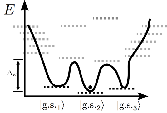
Figure 1: We show the quantum energy spectrum as several discrete energy levels in terms of horizontal dashed lines (- - -). The approximate semi-classical energy potential are drawn in terms of the continuous solid black curve. The vertical axis shows the energy value $E$. The horizontal axis illustrates their different quantum numbers, which can be, for example, (1) different eigenvectors spanning different subspaces in the Hilbert space; or (2) different spin/angular/spacetime momenta, etc. This figure shows 3 topological degenerate ground states $|\text{g.s.}_{1}\rangle$, $|\text{g.s.}_{2}\rangle$ and $|\text{g.s.}_{3}\rangle$ with the dark gray horizontal dashed lines (- - -) for their energy levels — Their energy levels only need to be approximately the same (within the order of $e^{-\#V}$ where $V$ is the system size), but they remain topologically robust. Namely, only via the insertion of the extended operator shown in eqn. (1.5) winding around a non-contractible cycle can the $|\text{g.s.}_{2}\rangle$ tunnel to the other sectors, even though their energy levels are nearly the same. The energy barrier is proportional to the cost of creating two anyonic excitations at the end of extended operators $W$ in eqn. (1.5). This energy barrier $\Delta_{E}$ naively seems to be infinite in TQFT, but it is actually of a finite order $\Delta_{E}\simeq 4J$ where $J$ is the lattice coupling constant in the UV complete lattice (e.g. in Kitaev’s toric code [28] or more general twisted quantum double models [29, 30]). In reality, as an example in 2+1D, the 3 topological degenerate ground states on a $T^{2}_{\text{space}}\times S^{1}_{\text{time}}$ can be induced from the filling fraction $\nu=\frac{1}{3}$-Laughlin fractional Quantum Hall states from electrons, or a $U(1)_{3}$-Chern-Simons theory at the deep IR. Further illustration is shown in Fig. 2

However, distinct vacuum sectors can be unitarily deformed into each other only through extended operators $W$ (line and surface operators, etc.) winding nontrivial cycles (1-cycle, 2-cycle, etc.) along compact directions of space. In the case that extended operator $W$ is a line operator, the insertion of $W$ can be understood as the process of creation and annihilation of a pair of anyonic excitations. Namely, a certain well-designed extended operator $W$ can indeed connect two different ground states/vacua, $|\text{g.s.}_{\alpha}\rangle$ and $|\text{g.s.}_{\beta}\rangle$, inducing nontrivial correlators:

$$\langle\text{g.s.}_{\alpha}|W(\gamma)|\text{g.s.}_{\beta}\rangle\to\text{finite}\neq 0.$$ (1.5)

Again $|\text{g.s.}_{\alpha}\rangle$ means the ground state $\alpha$ among the total GSD sector, and $\gamma$ is a nontrivial cycle in the space. Therefore, computing GSD also serves us as important data for counting extended operators, thus counting distinct types of anyonic particles or anyonic strings, etc.

Different degenerate ground states can also be regarded as different approximate vacuum sectors in particle physics or in cosmology, see Fig. 1 for further explanations and analogies. Therefore, in summary, our results might be of general interests to the condensed matter, mathematical physics, high-energy particle theory and quantum gravity/cosmology community.

1.2 The plan of the article and a short summary

First, in Sec.2, we describe how formal mathematical idea of decategorification can be helpful to organize the topological data. In down-to-earth terms, we can decompose GSD data read from $d+1$D into a direct sum of several sub-dimensional GSD sectors in $d$D, by compactifying one of the spatial dimensions on a small circle.

Then in Sec. 3 and Sec. 4, we start from more familiar discrete gauge theories. For example, the ${\mathbb{Z}}_{N}$ gauge theory[31, 32]. More generally, we can consider the twisted discrete gauge theories, known as Dijkgraaf-Witten (DW) gauge theories[33]. These are bosonic TQFTs that can be (1) realized at the UV lattice cutoff through purely bosonic degrees of freedom, and (2) defined on both non-spin and spin manifold. We will study the GSD for these bosonic TQFTs.

There has been a lot of recent progress on understanding bosonic Dijkgraaf-Witten (DW) gauge theories in terms of continuum TQFTs. However, to our best knowledge, so far there are no explicit calculations of GSD from the continuum field theories for the proposed non-Abelian DW gauge theories. Our work will fill in this gap for better analytical understanding, by computing non-Abelian GSD using continuum TQFTs, that matches precisely to the predictions of GSD computed from the original Dijkgraaf-Witten group cohomology data: Discrete cocycle path integrals. We present these results in Sec. 3 and Sec. 4.

By non-Abelian topological orders, we mean that some of the following properties are matched:

• The GSD $=Z(S^{d}\times S^{1};\sigma_{1},\sigma_{2},\sigma_{3},\dots)=\dim{\cal H}_{S^{d};\sigma_{1},\sigma_{2},\sigma_{3},\dots}$ computed on a sphere $S^{d}$ with operator insertions (or the insertions of anyonic particle/string excitations on $S^{d}$) have the following behavior: (1) $Z(S^{d}\times S^{1};\sigma_{1},\sigma_{2},\sigma_{3},\dots)=\dim{\cal H}_{S^{d};\sigma_{1},\sigma_{2},\sigma_{3},\dots}$ will grow exponentially as $k^{n}$ for a certain set of large $n$ number of insertions, for some number $k$. The anyonic particle causes this behavior is called non-Abelian anyon or non-Abelian particle. The anyonic string causes this behavior can be called non-Abelian string [10, 37]. (2) $Z(S^{d}\times S^{1};\sigma_{1},\sigma_{2},\sigma_{3})=\dim{\cal H}_{S^{d};\sigma_{1},\sigma_{2},\sigma_{3}}>1$ for a certain set of three insertions.

• The Lie algebra of underling Chern-Simons theory is non-Abelian, if such a Chern-Simons theory exists.

• The GSD $Z(T^{d}\times S^{1})=\dim{\cal H}_{T^{d}}$ for a discrete gauge theory of a gauge group $G$ on $T^{d}$ spatial torus, behaves as GSD$<|G|^{d}$, i.e. reduced to a smaller number than Abelian GSD. This criterion however works only for 1-form gauge theory.

Demonstrating that $Z(M^{d}\times S^{1})$ effectively counts the dimensions of Hilbert space on $M^{d}$, provides a more convincing quantum mechanical understanding of continuum/cochain TQFTs. By computing the following data, independently without using particular triangulations of spacetime,

1. GSD data, counting dimensions of Hilbert space,

2. Various braiding statistics and link invariants derived in [7],

for Abelian or non-Abelian cases, we solidify and justify their continuum/cochain field theory descriptions of both Abelian or non-Abelian Dijkgraaf-Witten theories, as we show that the data are matched with the calculations based on triangulations [10, 38]. Our present results combined together with Ref. [7] positively support the previous attempts based on continuum TQFTs [39, 40, 41, 12, 36, 42, 43, 44, 45, 46, 47, 48, 38, 49, 50, 51]. Various data derived from continuum TQFTs can be checked and compared through the discrete cocycle and lattice formulations [29, 52, 53, 8, 9, 10, 30, 37, 54, 55, 56, 57].

In Sec. 5, we study fermion TQFTs (the so-called spin-TQFTs) and their GSD. These fermion spin TQFTs are much subtler. They are obtained from dynamically gauging the global symmetry of fermionic SPTs [7]. Although the original fermionic SPTs and the gauged fermionic spin TQFTs have the UV completion on the lattice, the effective IR field theory may not necessarily guarantee good local action descriptions. These somehow non-local topological invariants include, for example, Arf-Brown-Kervaire (ABK) and $\eta$ invariants, intrinsic to the fermionic nature of systems. Nevertheless, there are still well-defined partition functions/path integrals and we can compute explicit physical observables. Our examples include intrinsically interacting 3+1D and 2+1D fermionic SPTs (fSPTs) as short-range entangled (SRE) states, and their dynamically gauged spin-TQFTs as long-range entangled (LRE) states. Recently, Ref. [58, 59, 60, 61] also explore the related interacting 3+1D fSPTs protected by the symmetry of finite groups. In Sec. 5, we will briefly comment the relations between our work and Ref. [58, 59, 60, 61].

In Sec. 6, we explore dimensional reduction scheme of partition functions. This section is based on the abstract and general thinking in Sec. 2 on (de)categorification. We implement it on explicit examples, in Sec. 3 and 4 on bosonic TQFTs and in Sec. 5 on fermionic TQFTs.

In Sec. 7, we mainly consider the long-range entangled (LRE) topologically-ordered bulk and boundary systems, denoted as LRE/LRE bulk/boundary for brevity. The LRE/LRE bulk/boundary systems can be obtained from dynamically gauging the bulk and unifying boundary conditions of symmetry-extension and symmetry-breaking introduced in Ref. [26]. In contrast, we will also compare the systems of LRE/LRE bulk/boundary to those of SRE/SRE bulk/boundary and SRE/LRE bulk/boundary.

In Sec. 8, we conclude with various remarks on long-range entanglements and entanglement entropy, and implications for the studied systems in various dimensions.

1.3 Topological Boundary Conditions: Old Anyonic Condensation v.s. New Condensation of Composite Extended Operators

Sec. 7 offers a mysterious and exotic new topological boundary mechanism, worthwhile enough for us to summarize its message in Introduction first. An important feature of LRE/LRE bulk/boundary is that both the bulk and boundary can have deconfined anyonic excitations. The anyonic excitations are 0D particles, 1D strings, etc., which can be regarded as the energetic excitations at the ends of extended operators supported on 1D lines, 2D surfaces, etc.

In contrast to the past conventional wisdom which suggests that the LRE topological gapped boundary is defined through the condensation of certain anyonic excitations, we emphasize that there are some additional subtleties and modifications needed. The previously established folklore that suggests the topological gapped boundary conditions are given by anyon condensation ([62, 63, 64, 25, 65, 66, 21], also References therein a recent review [67]), Lagrangian subgroups or their generalization [24, 19, 68, 69, 70, 22]. For example, in 1+1D boundary of 2+1D bulk (say $\Sigma^{2}=\partial M^{3}$ is the boundary), the condensation of anyons suggest their line operators can end on the boundary $\Sigma^{2}$. Formally, we have boundary conditions of the following type:

$$\left.\sum_{i}q_{i}A_{i}\right|_{\Sigma^{2}}=0,$$ (1.6)

or similar, that is certain linear combinations of line operators (with coefficients $q_{i}$) can end on ${\Sigma^{2}}$. Here and below $A_{i}$ denote 1-form gauge fields.

For example, if we consider a ${\mathbb{Z}}_{N}$ gauge theory of action $\int{\frac{N}{2\pi}{B\wedge dA}}$ (i.e. ${\mathbb{Z}}_{N}$ toric code /topological order) on any $d+1$D $M^{d+1}$, we can determine two types of conventional topological gapped boundary conditions on $\Sigma^{d}=\partial M^{d+1}$:

1. By condensations of ${\mathbb{Z}}_{N}$ charge (i.e. the electric $e$ particle attached to the ends of ${\mathbb{Z}}_{N}$ Wilson worldline $\int A$ of 1-form gauge field), set by:

$$\left.A\right|_{\Sigma^{d}}=0,\;\;\;\;\;\;\text{ as ${\mathbb{Z}}_{N}$ charge $e$ condensed on ${\Sigma^{d}}$}.$$ (1.7)

2. By condensations of ${\mathbb{Z}}_{N}$ flux (i.e. the magnetic $m$ flux attached to the ends of ${\mathbb{Z}}_{N}$ ’t Hooft worldvolume $\int B$ of $(d-1)$-form gauge field), with the $m$-condensed boundary set by:

$$\left.B\right|_{\Sigma^{d}}=0,\;\;\;\;\;\;\text{ as ${\mathbb{Z}}_{N}$ flux $m$ condensed on ${\Sigma^{d}}$}.$$ (1.8)

The UV lattice realization of above two boundary conditions are constructed in the Kitaev’s toric code [71] as well as Levin-Wen string-net [25]. The two boundary conditions in eqn. (1.7) and eqn. (1.8) are incompatible. Namely, each given physical boundary segment can choose either one of them, either $e$ or $m$ condensed but not the other.

However, in Sec. 7, we find that the usual anyon condensations like $\left.\sum_{i}q_{i}A_{i}\right|_{\Sigma^{d}}=0$ (including eqn. (1.7) and eqn. (1.8)) are not sufficient. We find that there are certain exotic, unfamiliar, new topological boundary conditions on 2+1D boundary of 3+1D bulk, such that neither $\left.A_{i}\right|_{\Sigma^{3}}=0$ nor $\left.A_{j}\right|_{\Sigma^{3}}=0$, but only the composite of extended operators can end on the boundary,

$$\left.{A_{i}\cup A_{j}}\right|_{\Sigma^{3}}=0.$$ (1.9)

Here $\cup$ is a cup product. Heuristically, we interpret these types of topological boundary conditions as the condensation of composite objects of extended operators. Here on a 2+1D boundary of a certain 3+1D bulk, we have a string-like composite object formed by a set of particles. The 1D string-like composite object is at the ends of 2D worldsheet $A_{i}\cup A_{j}$. The set of 0D particles we refer to are the ends of 1D worldlines $A_{i}$ and $A_{j}$. The boundary condition $\left.{A_{i}\cup A_{j}}\right|_{\Sigma^{2}}=0$ is achieved neither by intrinsic 0D particle nor by intrinsic 1D string excitation condensation alone. We suggest, this exotic topological deconfined boundary condition may be interpreted as condensing certain composite 1D string formed by 0D particles.

In summary, in Sec. 7, we find that gauge symmetry-breaking boundary conditions are indeed related to the usual anyon condensation of particles/strings/etc. The gauge symmetry-extension of LRE/LRE bulk/boundary in Ref. [26] sometimes can be reduced to the usual anyon condensation story (e.g. for 2+1D bulk), while other times, instead of the condensations of a set of anyonic excitations, one has to consider condensations of certain composite objects of extended operators (e.g. for certain 3+1D bulk).

1.4 Tunneling topological vacua in LRE/LRE bulk/boundary/interface systems

(a)
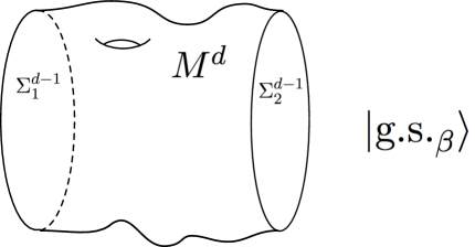
(b)

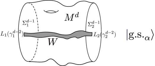
Figure 2: Illustration of tunneling between topological vacua, from $|\text{g.s.}_{\beta}\rangle$ to $|\text{g.s.}_{\alpha}\rangle$, via an extended operator $W$. In fig.(a), we see the topological vacuum in an original ground state $|\text{g.s.}_{\beta}\rangle$, where the spatial manifold $M^{d}$ is shown. On top of $M^{d}$, there are LRE/LRE bulk/boundary with topologically orders (TQFTs). In fig.(b), after inserting certain extended operator $W$ connecting two boundary components ($\Sigma_{1}^{d-1}$ and $\Sigma_{2}^{d-1}$), usually by an adiabatic process, we switch or tunnel to another topological vacuum $|\text{g.s.}_{\alpha}\rangle$. In the case of a closed manifold, the extended $W$ goes along a non-contractible cycle (representing a nontrivial element of the homology group of $M^{d}$).

We offer one last remark before moving on to the main text in Sec. 2. Similarly to eqn. (1.5), we can also interpret switching the topological sectors of gapped boundary/interface systems of Sec. 7, in terms of tunneling topological vacua by using extended operators $W$. The equation eqn. (1.5) still holds when when the operator $W$ has a support with two boundary components $\gamma_{1}^{d-2}$ and $\gamma_{2}^{d-2}$ that, in turn, support $(d-2)$D operators $L_{1}/L_{2}$ and lie in two different boundary components/interfaces $\Sigma_{1}^{d-1}$ and $\Sigma_{2}^{d-1}$ of the spatial manifold:

$$\left.\langle\text{g.s.}_{\alpha}|L_{1}(\gamma_{1})W(\gamma_{1},\gamma_{2})L_{2}(\gamma_{2})|\text{g.s.}_{\beta}\rangle\right|_{\gamma_{j}^{d-2}\subset\Sigma_{j}^{d-1}}\to\text{finite}\neq 0.$$ (1.10)

Here the open spacetime manifold $\partial M^{d}$ has two or more boundary components

$$\partial M^{d}=\Sigma_{1}^{d-1}\sqcup\Sigma_{2}^{d-1}\sqcup\dots.$$

As usual, $\sqcup$ means disjoint union. Physically, by moving certain (anyonic) excitations of either the usual extended operators or the composite extended operators, from one boundary component $\Sigma_{1}^{d-1}$ to another boundary component $\Sigma_{2}^{d-1}$, we have switched the ground state between $|\text{g.s.}_{\alpha}\rangle$ and $|\text{g.s.}_{\beta}\rangle$, as eqn. (1.10) suggested, shown in Fig. 2.

This idea is deeply related to Laughlin’s thought experiment in condensed matter [72]: Adiabatically dragging fractionalized quasiparticle between two edges of the annulus via threading a background magnetic flux through the hole of annulus — this would change the ground state sector. This also lays the foundation of Kitaev’s fault-tolerant quantum computation in 2+1D by anyons [28]. Various applications can be found in [73, 19, 74, 21] and references therein. In our work, we generalize the idea to any dimensions. This idea in some sense also helps us to the counting of GSD and extended operators for LRE/LRE bulk/boundary systems.

2 Strategy: (De)Categorification, Dimensional Decomposition and Intuitive Physical Picture

In this section, we address physical ideas of dimensional reduction/extension of partition functions and topological vacua (GSD), and their relations to formal mathematical ideas of decategorification/categorification. These ideas are actually relevant to physical phenomena measurable in a laboratory, see Fig. 3. In condensed matter, the related idea of dimensional reduction was first studied in [75] and [10] for 3+1D bulk theories. Here we apply the idea to an arbitrary dimension. Later, gathering the concrete calculations in Sec. 3, 4 and 5, we will implement the strategy outlined here on those examples in Sec. 6.

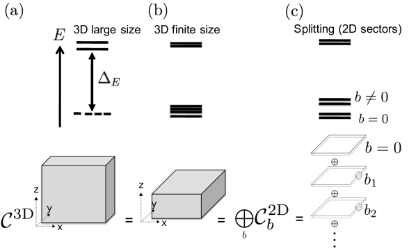
Figure 3: Relating the dimensional reduction and (de)categorification to measurable physical quantum phenomena in the laboratory. The top part of the subfigure (a) shows the bulk energy spectrum $E$ with energy gap $\Delta_{E}$, in the large 3+1D size limit. The bottom part shows in grey color a 3D spatial sample on $T^{3}$ torus with large compact circles in all $x,y,z$ directions. The degenerate zero modes in the energy spectrum are due to the non-trivial topological order (described by a TQFT) of the quantum system. The subfigure (b) shows that the energy spectrum slightly splits due to finite size effect, but its approximate GSD is still topologically robust. The subfigure (c) shows the system on $T^{3}$ torus in the limit of small circle in the $z$ direction. The energy spectrum forms several sectors, that can be labeled by a quantum number $b$ associated to the holonomy $\oint_{S^{1}_{z}}A$ of gauge field $A$ along $z$ (or a background flux through the compact circle) as $b\sim\oint A$. See more detailed explanation in the main text.

Fig. 3 shows how the energy spectrum of a topologically ordered sample (shown as a cuboid in grey color) effectively described by an underlying TQFT gets affected by the system size and by the holonomies of gauge fields through the compact circles. The topologically ordered cuboid is displayed in the real space. The energy eigenstates live in the Hilbert space. The energy spectrum can be solved from a quantum mechanical Hamiltonian system.

Fig. 3 (a) shows the system at a large or infinite size limit in the real space (in the case when the spatial manifold is $M^{d}=T^{d}$, $d=3$ with every $S^{1}$ circle size $\to\infty$), when the topological degeneracy of zero energy modes becomes almost exact. The zero modes are separated from higher excitations by a finite energy gap $\Delta_{E}$.

Fig. 3 (b) shows the system at finite size in real space. The GSD becomes approximate but still topologically robust.

Fig. 3 (c) shows that, when $M^{d}=M^{d-1}\times S^{1}_{z}$ (in the case $M^{d}=T^{3}$) and the compact $z$ direction’s $S^{1}_{z}$ circle becomes small, the approximate zero energy modes form several sectors, labeled by quantum number $b$ associated to the holonomy $b\sim\oint_{S^{1}_{z}}A$ of a gauge field $A$ along $z$ (or a background flux threading via the compact circle). In $d+1$-dimensions, this means that

$$\text{GSD}_{T^{d},\;d+1\text{D-TQFT}}=\sum_{b}\text{GSD}_{T^{d-1},\;(d-1)+1\text{D-TQFT}^{\prime}(b)}.$$ (2.1)

The energy levels within each sector of $\text{GSD}_{T^{d},(d-1)+1\text{D-TQFT}^{\prime}(b)}$ are approximately grouped together. However, energy levels of different sectors, labeled by different $b$, can be shifted upward/downward differently due to tuning the quantum number $b\sim\oint_{S^{1}_{z}}A$. This energy level shifting is due to Aharonov-Bohm type of effect. This provides the physical and experimental meanings of this decomposition.

More generally, one can consider the decomposition of the (zero mode part of the) Hilbert space of a $d+1$-dimensional TQFT on $M^{d-1}\times S^{1}$ into the Hilbert spaces of $(d-1)+1$-dimensional TQFTs on $M^{d}$:

$${\cal H}_{d+1\text{D-TQFT}}(M^{d-1}\times S^{1})=\bigoplus_{b}{\cal H}_{(d-1)+1\text{D-TQFT}^{\prime}(b)}(M^{d-1})$$ (2.2)

Note that (2.2) in principle contains more information than just the decomposition of the GSDs (as in (2.1) for $M^{d-1}=T^{d-1}$). This is because the Hilbert space ${\cal H}_{M^{d}}$ of a $d+1$-dimensional TQFT on $M^{d}$ forms a representation of the mapping class group of $M^{d}$, MCG($M^{d}$). Therefore (2.2) should be understood as the direct sum decomposition of representations of MCG($M^{d-1}$). This generalizes the relation of MCG to the dimensional decomposition scheme proposed in [76]. Examples in [10, 75] show that for a 3+1D to 2+1D decomposition, we indeed have the modular $S$ and $T$ representation of $\text{MCG}(T^{n})=SL(n,{\mathbb{Z}})$ data decomposition: $S^{xy,3\text{D}}=\bigoplus_{b}S^{xy,2\text{D}}_{b}$ and $T^{xy,3\text{D}}=\bigoplus_{b}T^{xy,2\text{D}}_{b}$ on a 2D spatial torus $T^{2}_{xy}$.

The statement can be made more precise in the case when the $d+1$-dimensional TQFT is realized by gauging a certain SPT with finite abelian (0-form) symmetry $G$. Suppose that other (ungauged) symmetries of the theory are contained in $H$, an extension of $SO$ (or $O$ when there is time-reversal symmetry) structure group of a space-time manifold. For example, when there is ${\mathbb{Z}}_{2}^{f}$ fermionic parity, one considers manifolds with Spin-structure. The corresponding SPT state then are classified by

$$\Omega^{d+1}_{H}(BG):=\text{Hom}(\Omega^{H}_{d+1}(BG),U(1)),$$ (2.3)

where $\Omega^{H}_{d+1}(BG)$ is the bordism group of manifolds with $H$-structure (e.g. $H=\text{Spin}$) [77, 78, 79] and equipped with maps to $BG$ (the classifying space of $G$).

Then, for an SPT state corresponding to a choice

$$\mu\in\Omega^{d+1}_{H}(BG),$$ (2.4)

the partition function of the corresponding gauged theory on a closed $d+1$-manifold is given by

$$Z_{\mu}(M^{d+1}):=\frac{1}{|G|^{|\pi_{0}(M^{d+1})|}}\sum_{a_{d+1}\in H^{1}(M^{d+1},G)}\mu([(M^{d+1},a_{d+1})])$$ (2.5)

where the pair $(M^{d+1},a_{d+1})$, a $(d+1)$-manifold with $H$-structure and a map $M_{d+1}\rightarrow BG$, represents an element in $\Omega^{H}_{d+1}(BG)$. Here and below we use one-to-one correspondence between homotopy classes of maps $M^{d+1}\rightarrow BG$ and elements of $H^{1}(M^{d+1},G)$. Note that the choice of $\mu$ can be understood as the choice of the action for finite group gauge theory: $\mu([(M^{d+1},a)])\equiv e^{iS(M^{d+1},a_{d+1})}\in U(1)$.

Suppose $H$-structures on $M^{d}$ and $S^{1}$ define $H$-structure on $M^{d}\times S^{1}$ (this is true for $H$=Spin example). Then one can consider the following map for a given element $b\in G$:

$$\begin{array}[]{cccc}\phi_{b}:&\Omega^{H}_{d}(BG)&\longrightarrow&\Omega^{H}_{d+1}(BG)\\ &[(M^{d},a_{d})]&\longmapsto&[(M^{d}\times S^{1},a_{d}\oplus(\underbrace{b\oplus\ldots\oplus b}_{|\pi_{0}(M^{d})|}))]\end{array}$$ (2.6)

where we used that $H^{1}(M^{d}\times S^{1})\cong H^{1}(M^{d})\oplus G^{|\pi_{0}(M^{d})|}$. It is easy to see that the map above is well defined, that is the image of $[(M^{d},a_{d})]$ does not depend on the choice of the representative $(M^{d},a_{d})$ in $\Omega^{H}_{d}(BG)$.

From the definition of gauged SPTs (2.5), it follows that for connected closed manifolds we have the following relation

$$\left.Z_{\mu}(M^{d}\times S^{1})\right|_{|\pi_{0}(M^{d})|=1}=\sum_{b\in G}Z_{\phi_{b}^{*}(\mu)}(M^{d}).$$ (2.7)

That is the partition function of the gauged $d+1$-dimensional SPT labeled by $\mu\in\Omega^{d+1}_{H}(BG)$ is given by the sum of gauged $d$-dimensional SPTs labeled by $\phi^{*}_{b}(\mu)\in\Omega^{d}_{H}(BG)$.

Similarly, for Hilbert spaces of the corresponding TQFTs we have

$$\left.{\cal H}_{\mu}(M^{d-1}\times S^{1})\right|_{|\pi_{0}(M^{d-1})|=1}=\bigoplus_{b\in G}{\cal H}_{\phi_{b}^{*}(\mu)}(M^{d-1}).$$ (2.8)

For a connected bordism $N^{d}$, $\partial N^{d}=\big{(}\sqcup_{i}(-M_{i}^{d-1})\big{)}\sqcup\,\big{(}\sqcup_{j}\tilde{M}_{j}^{d-1}\big{)}$ we then have

$$\left.Z_{\mu}(N^{d}\times S^{1})\right|_{|\pi_{0}(N^{d})|=1}=\mathfrak{i}_{\text{diag}}\circ\left(\bigoplus_{b\in G}Z_{\phi^{*}_{b}(\mu)}(N^{d})\right)\circ\mathfrak{pr}_{\text{diag}}$$ (2.9)

where

$$\begin{array}[]{cccc}Z_{\mu}(N^{d}\times S^{1}):&\otimes_{i}{\cal H}_{\mu}(M_{i}^{d-1})&\longrightarrow&\otimes_{j}{\cal H}_{\mu}(\tilde{M}_{j}^{d-1})\\ Z_{\phi^{*}_{b}(\mu)}(N^{d}\times S^{1}):&\otimes_{i}{\cal H}_{\phi^{*}_{b}(\mu)}(M_{i}^{d-1})&\longrightarrow&\otimes_{j}{\cal H}_{\phi^{*}_{b}(\mu)}(\tilde{M}_{j}^{d-1})\end{array}$$ (2.10)

and

$$\begin{array}[]{cccc}\mathfrak{i}_{\text{diag}}:&\bigoplus\limits_{b\in G}\bigotimes\limits_{j}{\cal H}_{\phi^{*}_{b}(\mu)}(\tilde{M}_{j}^{d-1})&\longrightarrow&\bigotimes\limits_{j}\bigoplus\limits_{b_{j}\in G}{\cal H}_{\phi^{*}_{b_{j}}(\mu)}(\tilde{M}_{j}^{d-1})=\bigotimes\limits_{j}{\cal H}_{\mu}(\tilde{M}_{j}^{d-1})\\ \mathfrak{pr}_{\text{diag}}:&\bigotimes\limits_{i}{\cal H}_{\mu}({M}_{i}^{d-1})=\bigotimes\limits_{i}\bigoplus\limits_{b_{i}\in G}{\cal H}_{\phi^{*}_{b_{i}}(\mu)}({M}_{i}^{d-1})&\longrightarrow&\bigoplus\limits_{b\in G}\bigotimes\limits_{i}{\cal H}_{\phi^{*}_{b}(\mu)}({M}_{i}^{d-1})\\ \end{array}$$ (2.11)

are inclusion of the diagonal and projection onto the diagonal.

Let us denote the TQFT functor (in the usual Atiyah’s meaning) for the (d+1)-dimensional gauged SPT labeled by $\mu$ as ${\cal C}^{d\text{D}}_{\mu}$ (so that its value on objects is given by ${\cal H}_{\mu}(\bullet)$ and its value on morphisms is $Z_{\mu}(\bullet)$). Then throughout the paper we will often write simply

$${\cal C}^{d\text{D}}_{\mu}=\bigoplus_{b\in G}{\cal C}^{(d-1)\text{D}}_{\phi^{*}_{b}(\mu)}$$ (2.12)

by which we actually mean that the functors satisfy relations (2.7), (2.8), (2.9). We thus decompose a $(d+1)$D-TQFT to many sectors of $((d-1)+1)$D-TQFT^′ labeled by $b$, in the topological vacua subspace within the nearby lowest energy Hilbert space. We mark that the related ideas of dimensional decomposition scheme are explored in [80, 81, 82, 83].

Relation (2.7) can also be interpreted as follows:

$$\sum_{b}Z_{\phi^{*}_{b}(\mu)}(M^{d})=Z_{\mu}(M^{d}\times S^{1})={\mathrm{Tr}}_{{\cal H}_{\mu}(M^{d})}1.$$ (2.13)

That is, the trace over the Hilbert space of $d+1$-dimensional TQFT has interpretation of sum over the partition functions of $d$-dimensional TQFTs. This is an example of the general notion of decategorification in mathematics, where the vectors space are replaced by numbers. The inverse, that is a lift of numbers to vector spaces is known as categorification. Note that even though the partition function of a single $d$-dimensional TQFT^′ in the sum above cannot be categorified (i.e. interpreted as a trace over some Hilbert space), a particular sum of them can be. The notion of (de)-categorification can be extented to the level of the extended TQFT functors. In particular, (2.8) can be interpreted as

$$K^{0}(\text{BCond}_{\mu}(M^{d-1}))=\bigoplus_{b\in G}{\cal H}_{\phi_{b}^{*}(\mu)}(M^{d-1})$$ (2.14)

where $\text{BCond}_{\mu}(M^{d-1})$ is the category of boundary conditions of the $(d+1)$-dimensional TQFT (obtained by gauging SPT labeled by $\mu$) on $M^{d-1}$ and $K^{0}$ is the Grothendieck group.

Note that in the case of fermionic theories the Hilbert spaces in (2.2) have an additional structure: ${\mathbb{Z}}_{2}^{f}$-grading (see section 5 for details).

3 Bosonic TQFTs and Ground State Degeneracy

In this section we compute the ground state degeneracy (GSD, or, equivalently, the vacuum degeneracy) of some topological field theories, using the strategy and the set up similar to the one in [7]. We will consider TQFTs with a continuum field description in terms of $n$-form gauge fields. The level-quantization constraint for such theories is derived and given in [12]. Below we compute the GSD on a spatial manifold ${M}^{d}$ via the absolute value of the partition function ${Z}$ on a spacetime manifold ${M}^{d}\times S^{1}$ based on its relation of to the dimension of Hilbert space ${\cal H}$:

$$\text{GSD}_{M^{d}}=\dim{\cal H}_{M^{d}}=Z(M^{d}\times S^{1}).$$

As a warm-up, we start with (untwisted) ${\mathbb{Z}}_{N}$ gauge theory[31], also known as ${\mathbb{Z}}_{N}$ spin liquid[84], ${\mathbb{Z}}_{N}$ topological order[85], or ${\mathbb{Z}}_{N}$ toric code[28]. Then we proceed to more general twisted discrete gauge theories: bosonic Dijkgraaf-Witten (DW) gauge theories. In most of the cases we consider the torus as the spatial manifold for simplicity:

$$\text{GSD}_{T^{d}}=\dim{\cal H}_{T^{d}}=|Z(T^{d+1})|.$$

Below we use the notation $N_{ijk\dots}\equiv\gcd(N_{i},N_{j},N_{k},\dots)$. We will always use $A$ to denote a 1-form gauge field, while $B$ can be a higher-form gauge field. In most cases, without introducing ambiguity, we omit the explicit wedge product $\wedge$ between differential forms. We will also often omit the explicit summations over the indices $I,J,K,\ldots$ in the formulas. We note that related calculations of bosonic GSD are also derived based on independent and different methods in [10, 38, 86]. Some of the main results of this section are briefly summarized in Table 1.

Dim	gauge group $G$	$\begin{array}[]{c}\text{Action}\\ (\text{Local})\end{array}$	$\text{GSD}_{T^{d}}$	$\text{GSD}_{S^{d-2}\times S^{1}}$
any D	$\prod_{I}{\mathbb{Z}}_{N_{I}}$	$\int\frac{N_{I}}{2\pi}{B^{I}dA^{I}}$	$|G|^{d}$	–
2+1D	$U(1)^{n}$ (level $K$)	$\int\frac{K_{IJ}}{4\pi}A^{I}dA^{J}$	$|\det K|$	–
2+1D	$\prod_{I}{\mathbb{Z}}_{N_{I}}$	$\int\frac{N_{I}}{2\pi}{B^{I}dA^{I}}+{\frac{p_{IJ}}{4\pi}}A^{I}dA^{J}$	$|G|^{2}$	–
2+1D	$\underset{{I=1,2,3}}{\prod}{\mathbb{Z}}_{N_{I}}$	$\int\frac{N_{I}}{2\pi}{B^{I}dA^{I}}+{\frac{N_{1}N_{2}N_{3}\;p}{{(2\pi)^{2}}N_{123}}}A^{1}A^{2}A^{3}$	$N^{4}+N^{3}-N$	–
3+1D	$\underset{{I=1,2,3}}{\prod}{\mathbb{Z}}_{N_{I}}$	$\int\frac{N_{I}}{2\pi}{B^{I}dA^{I}}{{+}}\frac{N_{I}N_{J}\;p_{IJK}}{{(2\pi)^{2}}N_{IJ}}A^{I}A^{J}dA^{K}$	$|G|^{3}$	$|G|$
3+1D	$\underset{{I=1,2,3,4}}{\prod}{\mathbb{Z}}_{N_{I}}$	$\int\frac{N_{I}}{2\pi}{B^{I}dA^{I}}+{\frac{N_{1}N_{2}N_{3}N_{4}\;p}{{(2\pi)^{3}}N_{1234}}}A^{1}A^{2}A^{3}A^{4}$	$\begin{matrix}N^{10}+N^{9}+N^{8}-N^{7}\\ -N^{6}-N^{5}+N^{3}\end{matrix}$	$|G|$
3+1D	$\underset{{I}}{\prod}{\mathbb{Z}}_{N_{I}}$	$\int\frac{N_{I}}{2\pi}B^{I}dA^{I}+\frac{p_{IJ}N_{I}N_{J}}{4\pi N_{IJ}}\,B^{I}B^{J}$	$\gcd(p,N)^{3}$	$\gcd(p,N)$
4+1D	$\underset{{I=1,\dots,5}}{\prod}{\mathbb{Z}}_{N_{I}}$	$\int\frac{N_{I}}{2\pi}{B^{I}dA^{I}}+{\frac{N_{1}N_{2}\dots N_{5}\;p}{{(2\pi)^{4}}N_{12345}}}A^{1}A^{2}A^{3}A^{4}A^{5}$	eqn. (4.4), eqn. (4.5)	$|G|$
$d$D	$\underset{{I=1,\dots,{d}}}{\prod}{\mathbb{Z}}_{N_{I}}$	$\int\frac{N_{I}}{2\pi}{B^{I}dA^{I}}+{\frac{N_{1}N_{2}\dots N_{d}\;p}{{(2\pi)^{d-1}}N_{1\dots d}}}A^{1}\dots A^{d}$	eqn. (4.7)	$|G|$

Table 1: Table of TQFTs and GSDs. For twisted gauge theories of Dijkgraaf-Witten (DW) theory, we will sometimes restrict to the case ${\mathbb{Z}}_{N_{1}}={\mathbb{Z}}_{N_{2}}={\mathbb{Z}}_{N_{3}}={\mathbb{Z}}_{N_{4}}=\dots\equiv{\mathbb{Z}}_{N}$ where $N$ is prime. Here $p$ is nontrivial and $\gcd(p,N)=1$ for those non-Abelian theories within DW theories; $G$ denotes the total finite gauge group in DW setup. Our derivations are based on continuum field descriptions. These results can be independently compared with discrete cocycle/cochain lattice path integral method in [10, 38].

3.1 $\int{BdA}$ in any dimension

To warm up, we evaluate the ground state degeneracy of the untwisted ${\mathbb{Z}}_{N}$ gauge theory in $d+1$D on torus $T^{d}$ as the partition function on $M^{d+1}=T^{d+1}$ spacetime in two different ways. In the first approach, we integrate out a $(d-1)$-form $B$ field which yields a condition of $A$ being flat together with quantization of its holonomies. We evaluate

$$\text{GSD}_{{T}^{d}} = \int[DB][DA]\exp[\int_{{T}^{d}\times S^{1}}{\frac{iN}{2\pi}{B\wedge dA}}]$$

$$= \int[DA]\;1|_{dA=0,\;\;\;\oint_{S^{1}\subset T^{d+1}}A=\frac{2\pi n_{\mu}}{N},\;\;\;n_{\mu}\in{\mathbb{Z}}_{N}}={\cal N}^{-1}\sum_{a\in H^{1}(M^{d+1},G)}1$$

$$= {\cal N}^{-1}\cdot{|H^{1}(M^{d+1},G)|}=\frac{|H^{1}(M^{d+1},G)|}{|H^{0}(M^{d+1},G)|}=\frac{N^{d+1}}{N}=N^{d}.$$

The $G={\mathbb{Z}}_{N}$ is the gauge group. The ${\cal N}^{-1}={|H^{0}(M^{d+1},G)|}^{-1}$ is the normalization factor that takes into account gauge redundancy of 1-form gauge field.

In the second approach, we integrate out a 1-form $A$ field which yields a flat $B$ condition together with quantization of its flux through any codimension-2 cycle $M^{d-1}\subset T^{d+1}$. We evaluate

$$\text{GSD}_{{T}^{d}} = \int[DB][DA]\exp[\int_{{T}^{d+1}}{\frac{iN}{2\pi}{B\wedge dA}}]$$

$$= \int[DB]\;1|_{dB=0,\;\;\;\oint_{M^{d-1}}B=\frac{2\pi n}{N},\;\;\;n\in{\mathbb{Z}}_{N}}$$

$$= {\cal N}^{-1}\cdot{|H^{d-1}(M^{d+1},G)|}=(\prod_{j=0}^{d-2}{|H^{d-2-j}(M^{d+1},G)|}^{(-1)^{j}})^{-1}{|H^{d-1}(M^{d+1},G)|}$$

$$= (N^{(-)^{d+1}{d+1\choose 0}}\dots N^{{d+1\choose d-3}}N^{-{d+1\choose d-2}})N^{{d+1\choose d-1}}=N^{d}.$$

The ${\cal N}^{-1}$ factor again takes into account the gauge redundancy of $(d-1)$-form gauge field $B$. The gauge transformation of $B\to B+d\lambda^{(d-2)}$ contains the $(d-2)$-form gauge parameter $\lambda^{(d-2)}$, whose gauge transformation allows $\lambda^{(d-2)}\to\lambda^{(d-2)}+d\lambda^{(d-3)}$ change with further lower form redundancy. Considering the gauge redundancy layer by layer, we obtain the ${\cal N}^{-1}$ factor in the third line in the above equation. The last equality uses $(1-s)^{d+1}={d+1\choose d+1}1^{d+1}-{d+1\choose d}s+{d+1\choose d-1}s^{2}+\dots+(-)^{d+1}{d+1\choose 0}s^{d+1}$ with $s=1$. The results of the above first and second approach match indeed, $\text{GSD}_{{T}^{d}}=|G|^{d}$.

3.2 $\int K_{IJ}A_{I}dA_{J}$, $\int{BdA}{{+}}AdA$ in 2+1D, $\int{BdA}{{+}}AAdA$ in 3+1D and $\int BdA+A^{d-1}dA$ in any dimension

First we compute the GSD of $\int\sum_{I=1}^{3}\frac{N_{I}}{2\pi}{B^{I}\wedge dA^{I}}{{+}c_{123}}A^{1}\wedge A^{2}\wedge dA^{3}$ (where $c_{123}=\frac{p_{123}N_{1}N_{2}}{(2\pi)^{2}N_{12}},\;p_{123}\in{\mathbb{Z}}$) theory on a torus. Other details of the theory are studied in [7], with the level-quantization constraint derived/given in [12].

$$\text{GSD}_{{T}^{3}} = \int[DB][DA]\exp[\int_{{T}^{3}\times S^{1}}{\frac{iN_{I}}{2\pi}{B^{I}\wedge dA^{I}}{{+i}c_{123}}A^{1}\wedge A^{2}\wedge dA^{3}}]$$

$$= \int[DA]\exp[\int_{{T}^{3}\times S^{1}}{{{i}c_{123}}A^{1}\wedge A^{2}\wedge dA^{3}}]|_{dA^{I}=0,\;\;\;\oint_{S^{1}}A^{I}=\frac{2\pi n_{I}}{N_{I}},\;\;\;n_{I}\in{\mathbb{Z}}_{N_{I}}}$$

$$= \sum_{n_{I,x},n_{I,y},n_{I,z}\in{\mathbb{Z}}_{N_{I}}}1=({N_{1}}{N_{2}}{N_{3}})^{3}=|G|^{3}.$$

We have used that $A$ satisfies the flatness condition in the second line, so all the configurations weigh with $\exp[\int{{i}c_{123}}A^{1}\wedge A^{2}\wedge dA^{3}]=1$. To sum over $\int[DA]$ in the partition function, we simply need to sum over all the possible holonomies $\oint_{S^{1}}A^{I}=\frac{2\pi n_{I}}{N_{I}}$ around every non-contractible directions. Similarly, for $\int\sum_{I=1}^{2}\frac{N_{I}}{2\pi}{B^{I}\wedge dA^{I}}{{+}c_{122}}A^{1}\wedge A^{2}\wedge dA^{2}$ theory, from the flatness condition on $A$ on the torus it follows that the partition function is given by

$$\text{GSD}_{{T}^{3}} = \sum_{n_{I,x},n_{I,y},n_{I,z}\in{\mathbb{Z}}_{N_{I}}}1=({N_{1}}{N_{2}})^{3}=|G|^{3}.$$ (3.4)

In 2+1D, the same strategy allows us to evaluate the GSD for $\int\sum_{I}\frac{N_{I}}{2\pi}{B^{I}\wedge dA^{I}}+\sum_{IJ}{c_{IJ}}A^{I}\wedge\hskip 1.0pt\mathrm{d}A^{J}$ ( $c_{IJ}=\frac{p_{IJ}}{4\pi},\;p_{IJ}\in{\mathbb{Z}}$) theory on a torus:

$$\text{GSD}_{{T}^{2}} = \int[DB][DA]\exp[\int_{{T}^{2}\times S^{1}}{\frac{iN_{I}}{2\pi}{B^{I}\wedge dA^{I}}{{+i}c_{IJ}}A^{I}\wedge\hskip 1.0pt\mathrm{d}A^{J}}]$$

$$= \int[DA]\exp[\int_{{T}^{2}\times S^{1}}{{{i}c_{IJ}}A^{I}\wedge\hskip 1.0pt\mathrm{d}A^{J}}]|_{dA^{I}=0,\;\;\;\oint_{S^{1}}A^{I}=\frac{2\pi n_{I}}{N_{I}},\;\;\;n_{I}\in{\mathbb{Z}}_{N_{I}}}$$

$$= \sum_{n_{I,x},n_{I,y}\in{\mathbb{Z}}_{N_{I}}}1=\prod_{I}({N_{I}})^{2}=|G|^{2}.$$

The result can be interpreted as the volume of the rectangular polyhedron with edges of sizes $N_{I}$ (each appearing twice). More generally, for an abelian Chern-Simons theory with matrix level $K$ [87], that is with the action $\int\frac{K_{IJ}}{4\pi}{A^{I}\wedge dA^{J}}$, the flatness condition is modified to $\sum_{J}K_{IJ}dA^{J}=0$. The result is then given by the volume of the polyhedron with edges given by column vectors of the matrix $K$:

$$\text{GSD}_{{T}^{2}}=|\det K|.$$ (3.6)

The calculation above can be easily generalized to the case of $d+1$-dimensional theory with the action of the form $\int BdA+A^{d-1}dA$. The result is $\text{GSD}_{T^{d}}=|G|^{d}$. This is in line with the fact that these theories are of abelian nature.

One can also obtain the GSD of the above theories based on the cochain path integral, see Ref. [38] on these Abelian TQFTs.

3.3 $\int{BdA}+\int BB$ in 3+1D

3.3.1 Twisted ${\mathbb{Z}}_{N}$ theory with a $B\wedge B$ term

We first consider a 3+1D action $\int\frac{N}{2\pi}{B\wedge dA}{{+}\frac{Np}{2\pi}}B\wedge B$. This theory has been considered in detail in [35] (appendix B). In the action above we chose a less refined level quantization, which is valid for any manifold possibly without a spin structure. For a non-spin bosonic TQFT, the level quantization can be easily derived based on [12]. For a spin fermionic TQFT, Ref.[35] provides a refined level quantization on a spin manifold, where the $p$ can take half integer values, namely we can redefine $p=p^{\prime}/2$ with an integer $p^{\prime}$. In short, we get $\int\frac{N}{2\pi}{B\wedge dA}{{+}\frac{Np^{\prime}}{4\pi}}B\wedge B$ where now $p^{\prime}\in{\mathbb{Z}}$. It is a spin TQFT when both $N$ and $p^{\prime}$ are odd. The gauge transformation is $B\to B+d\lambda$, $A\to A-2p\lambda+dg=A-p^{\prime}\lambda+dg$.

Using the approach similar to the one in the second part of section 3.1 we can evaluate its GSD on a 3-torus:

$$\text{GSD}_{{T}^{3}} = \int[DB][DA]\exp[\int_{{T}^{3}\times S^{1}}{\frac{iN}{2\pi}{B\wedge dA}{{+}\frac{iNp}{2\pi}}B\wedge B}]$$

$$= \int[DB]\exp[\int_{{T}^{3}\times S^{1}}{\frac{iNp}{2\pi}}B\wedge B]|_{dB=0,\;\;\;\oint_{M^{2}}B=\frac{2\pi n}{N},\;\;\;n\in{\mathbb{Z}}_{N}}$$

$$= {\cal N}^{-1}\sum_{n_{\alpha\beta}\in{\mathbb{Z}}_{N}}\exp[{{i}}\frac{2\pi(2p)}{N}(n_{xy}n_{zt}-n_{xz}n_{yt}+n_{yz}n_{xt})]$$

$$= {\cal N}^{-1}\sum_{n_{\alpha\beta}\in{\mathbb{Z}}_{N}}\exp[{{i}}\frac{2\pi({2}p/\gcd({2}p,N))}{(N/\gcd({2}p,N))}(n_{xy}n_{zt}-n_{xz}n_{yt}+n_{yz}n_{xt})]$$

$$= {\cal N}^{-1}(\frac{N\cdot N}{(N/\gcd({2}p,N))})^{3}=(\frac{N^{4}}{N})^{-1}(\frac{N\cdot N}{(N/\gcd({2}p,N))})^{3}=\gcd({2}p,N)^{3}=\gcd(p^{\prime},N)^{3}.$$

Where $n_{\alpha\beta}$ are fluxes of the field $B$ through 2-tori in the directions $\alpha,\,\beta$. The sum over $n_{\alpha\beta}$ factorizes into the product of sums over the pairs $n_{xy},n_{zt}$, $n_{xz},n_{yt}$ and $n_{yz},n_{xt}$. These sums can be interpreted as sums over integral points inside squares of size $N$. Each square has $N\cdot N$ area. We divide this area by $(N/\gcd(p^{\prime},N))$, since a summation of $(N/\gcd(p^{\prime},N))$ number of exponential factors gives one. We used the fact that $(p^{\prime}/\gcd(p^{\prime},N))$ and $(N/\gcd(p^{\prime},N))$ are relatively prime. The ${\cal N}^{-1}$ factor is derived from dividing by the number of 1-form gauge symmetries, $|H^{1}(M,G)|$ which is equal to $N^{4}$ on the ${{T}^{3}\times S^{1}}$, and then multiplying by the order of the gauge group, $|H^{0}(M,G)|=N$. This gives the normalization factor ${\cal N}^{-1}=1/(N^{4}/N)=1/N^{3}$, which accounts for the redundancy of “gauge symmetries” and “gauge symmetries of gauge symmetries.” Overall, we obtain $\text{GSD}_{{T}^{3}}=\gcd(p^{\prime},N)^{3}$ which is consistent with Ref.[35]. See [35] for the evaluation of partition function on other manifolds.

We can also use another independent argument based on Ref.[35] to verify the GSD obtained above. In Ref.[35], it was found that $\int{\frac{N}{2\pi}{B\wedge dA}{{+}\frac{Np^{\prime}}{4\pi}}B\wedge B}$ theory has a similar GSD as ${\mathbb{Z}}_{\gcd(N,p^{\prime})}$ gauge theory at the low energy. First, we know that the commutator between conjugate field and momentum operators is $[A(x),B(x^{\prime})]=\frac{i2\pi}{N}\delta{(x-x^{\prime})}$. At $p=0$, there is a 2-form global symmetry ${\mathbb{Z}}_{N}$ and a 1-form global symmetry ${\mathbb{Z}}_{N}$ generated by:

$$U=e^{i\oint_{\gamma}A},\;\;\;\;V=e^{i\oint_{\Sigma}B}.$$

At $p=0$, the symmetry transformation gives,

$$B \to UBU^{-1}=B-\frac{1}{N}\xi_{B},$$ (3.8)

$$A \to VAV^{-1}=A+\frac{1}{N}\zeta_{A},$$ (3.9)

with $\xi_{B}$ and $\zeta_{A}$ are flat and satisfying $\oint_{\Sigma}\xi_{B}=2\pi$ and $\oint_{\gamma}\zeta_{A}=2\pi$, so that $U^{N}=V^{N}=1$ and $UV=e^{\frac{i2\pi}{N}}VU$. The operators $U$ and $V$ can be referred to as the clock and the shift operators (like the angle and angular momentum operators). They generate $N$ distinct ground states along each non-contractible loop. On the other hand, when $p^{\prime}\neq 0$, we can consider an open cylindrical surface ($\Sigma$) operator with two ends on closed loops $\gamma$ and $\gamma^{\prime}$:

$$W=\exp[i\oint_{\gamma}A+ip^{\prime}\int_{\Sigma}B-i\oint_{\gamma^{\prime}}A].$$

The boundary components of $\Sigma$ are $\gamma$ and $\gamma^{\prime}$, which makes the operator gauge invariant under the gauge transformation. The closed line operator with $\exp[i\oint_{\gamma}A]$ can be defined whenever the contribution from the open surface part becomes trivial. Let $\Sigma_{1}$ and $\Sigma_{2}$ be two distinct surfaces bounded by $\gamma$ and $\gamma^{\prime}$ (i.e., $\partial\Sigma_{1}=\partial\Sigma_{2}=\gamma_{1}\cup(-\gamma_{2})$ where the minus sign indicates the opposite orientation), then $\Sigma_{1}-\Sigma_{2}$ is a closed surface, and we have $\int_{\Sigma_{1}}B-\int_{\Sigma_{2}}B=\frac{2\pi}{N}n$ with some $n\in{\mathbb{Z}}_{N}$, since $\oint_{\Sigma_{1}-\Sigma_{2}}B=\frac{2\pi}{N}n$. The minimum integer $I$ enforcing $Ip^{\prime}\int_{\Sigma_{1}-\Sigma_{2}}B={2\pi}$ is $I=\frac{N}{\gcd(p^{\prime},N)}$. This means that $\exp[i(I\oint_{\gamma}A+Ip^{\prime}\int_{\Sigma}B-I\oint_{\gamma^{\prime}}A)]$ does not depend on the choice of the open surface $\Sigma$, and we can view $\exp[i(I\oint_{\gamma}A+Ip^{\prime}\int_{\Sigma}B-I\oint_{\gamma^{\prime}}A)]$ as two deconfined line operators formally as $\exp[i(I\oint_{\gamma}A-I\oint_{\gamma^{\prime}}A)]$. Thus we can define the line operator alone as:

$$U=\exp[i\;I\oint_{\gamma}A]=e^{i\frac{N}{\gcd(p^{\prime},N)}\oint A},\;\;\;\;\text{with}\;\;\;\;U^{\gcd(p^{\prime},N)}=1.$$ (3.10)

The reasoning is, again, that since $\oint_{\gamma}A=\frac{2\pi}{N}n$ with some $n\in{\mathbb{Z}}_{N}$, then we have $U=\exp[i\frac{2\pi n}{\gcd(p^{\prime},N)}]$ satisfying $U^{\gcd(p^{\prime},N)}=1$.

The closed surface operator alone can be defined as:

$$V=\exp[i\oint_{\Sigma}B],\;\;\;\;\text{ while }V^{N}=1\text{ and }V^{p^{\prime}}=1,\;\;\;\;\text{ so }V^{\gcd(p^{\prime},N)}=1.$$ (3.11)

Here $V^{N}=1$ is due to $\oint_{\Sigma}B=\frac{2\pi}{N}n$. On the other hand, we can close the open surface by letting two closed curves ${\gamma}$ and ${\gamma^{\prime}}$ coincide, then the open surface operator $\exp[i\oint_{\gamma}A+ip^{\prime}\int_{\Sigma}B-i\oint_{\gamma^{\prime}}A]$ becomes the surface operator $\exp[ip^{\prime}\oint_{\Sigma}B]$. But the original open surface operator must be trivial (inside correlation functions) because the theory describes topological and gapped systems. This implies $W=1$ and thus $\exp[ip^{\prime}\oint_{\Sigma}B]=1\Rightarrow V^{p^{\prime}}=1$. The superposed conditions of $V^{N}=1$ and $V^{p^{\prime}}=1$, give the final finest constraint $V^{\gcd(p^{\prime},N)}=1$. Finally we obtain:

$$UV=e^{\frac{i2\pi}{\gcd(p^{\prime},N)}}VU,\;\;\;\;\text{ because of }[\frac{N}{\gcd(p^{\prime},N)}A(x),B(x^{\prime})]=\frac{i2\pi}{\gcd(p^{\prime},N)}\delta{(x-x^{\prime})}.$$

Thus the new clock and shift operators generate ${\gcd(p^{\prime},N)}$ distinct ground states along each non-contractible loop. For $\text{GSD}_{{T}^{3}}$ on a ${{T}^{3}}$ spatial torus with three spatial non-contractible loops, we obtain $\text{GSD}_{{T}^{3}}={\gcd(p^{\prime},N)}^{3}$ as in [35].

3.3.2 More general theory

We can also consider a more generic action $\int\sum_{I=1}^{2}\frac{N_{I}}{2\pi}{B^{I}\wedge dA^{I}}+{\frac{p_{12}N_{1}N_{2}}{2\pi N_{12}}}B^{1}\wedge B^{2}$ where $N_{12}\equiv{\gcd(N_{1},N_{2})}$ and $p_{12}$ can be a half-integer. Again we choose a less refined level quantization, which is true for any generic manifold without a spin structure. The gauge transformation is the following:

$$B^{I}\to B^{I}+d\lambda^{I},\;\;\;A^{1}\to A^{1}-p_{12}\frac{N_{1}}{N_{12}}\lambda+dg^{1},\;\;\;A^{2}\to A^{2}-p_{12}\frac{N_{2}}{N_{12}}\lambda+dg^{2}.$$ (3.12)

Again, we derive $\text{GSD}_{{T}^{3}}$ on a ${{T}^{3}}$ spatial torus:

$$\text{GSD}_{{T}^{3}} = \int[DB][DA]\exp[\int_{{T}^{3}\times S^{1}}{\frac{iN_{I}}{2\pi}{B^{I}\wedge dA^{I}}{{+}\frac{ip_{12}N_{1}N_{2}}{2\pi N_{12}}}B^{1}\wedge B^{2}}]$$

$$= \int[DB]\exp[\int_{{T}^{3}\times S^{1}}{+}\frac{ip_{12}N_{1}N_{2}}{2\pi N_{12}}B^{1}\wedge B^{2}]|_{dB^{I}=0,\;\;\;\oint_{M^{2}}B^{I}=\frac{2\pi n_{I}}{N_{I}},\;\;\;n_{I}\in{\mathbb{Z}}_{N}}$$

$$= {\cal N}^{-1}\sum_{n^{I}_{\alpha\beta}\in{\mathbb{Z}}_{N_{I}}}\exp[{{i}}\frac{2\pi(\frac{2p_{12}}{\gcd(2p_{12},N_{12})})}{(\frac{N_{12}}{\gcd(2p_{12},N_{12})})}(n_{xy}^{1}n_{zt}^{2}-n_{xz}^{1}n_{yt}^{2}+n_{yz}^{1}n_{xt}^{2}+n_{zt}^{1}n_{xy}^{2}-n_{yt}^{1}n_{xz}^{2}+n_{xt}^{1}n_{yz}^{2})]$$

$$= {\cal N}^{-1}(\frac{N_{1}\cdot N_{2}}{(N_{12}/\gcd(2p_{12},N_{12}))})^{6}=(\frac{|H^{1}(M,G)|}{|H^{0}(M,G)|})^{-1}\cdot(\frac{N_{1}\cdot N_{2}}{(N_{12}/\gcd(2p_{12},N_{12}))})^{6}$$

$$= \frac{N_{1}N_{2}}{N_{1}^{4}N_{2}^{4}}\cdot(\frac{N_{1}\cdot N_{2}}{(N_{12}/\gcd(2p_{12},N_{12}))})^{6}=(\frac{\operatorname{lcm}(N_{1},N_{2})}{\gcd(N_{1},N_{2})})^{3}\gcd({2}p_{12},N_{12})^{6}.$$

Similarly to Sec. 3.3.1, the ${\cal N}^{-1}$ factor is derived from dividing by the number of 1-form gauge symmetries, $|H^{1}(M,G)|$, and then multiplying by the order of the gauge group, $|H^{0}(M,G)|$. This accounts for the redundancy of “gauge symmetries” and “gauge symmetries of gauge symmetries.”

3.4 $\int{BdA}+\int AA$ in 1+1D

We consider the 1+1D TQFT with the action $\int\frac{N_{I}}{2\pi}{B^{I}\wedge dA^{I}}+\frac{p_{12}N_{1}N_{2}}{2\pi\,N_{12}}A^{1}\wedge A^{2}$. Locally B is a 0-form field and $A$ is a 1-form field. The level quantization is described in [12, 7]. This theory can be obtained by dynamically gauging an SPTs with the symmetry group $G_{s}=\prod_{I=1}^{2}{\mathbb{Z}}_{N_{I}}$ [36]. Its dimension of Hilbert space on ${S}^{1}$ is computed as a discrete sum, after integrating out $B$ field:

$$\text{GSD}_{{S}^{1}}={\cal N}^{-1}\sum_{\vec{n}_{I}\in{\mathbb{Z}}_{N_{I}}^{2}}\exp[-{{i}}p_{12}\frac{2\pi}{N_{12}}\det(\vec{n}_{1},\vec{n}_{2})].$$ (3.14)

Consider a specific example $N_{1}=N_{2}=N$ which is a prime number, so that $\gcd(p_{12},N)=1$. In this case,

$$\text{GSD}_{{S}^{1}} = {\cal N}^{-1}\sum_{\vec{n}_{I}\in{\mathbb{Z}}_{N}^{2}}\exp[-{{i}p_{12}}\frac{2\pi}{N}\det(\vec{n}_{1},\vec{n}_{2})]=\sum_{n_{2,x},n_{2,t}\in{\mathbb{Z}}_{N}}\delta({n}_{2,x})\delta({n}_{2,t})=1.\;\;\;\;\;\;\;\;\;\;$$ (3.15)

There is a unique ground state degeneracy without robust topological order in this case.

For more generic $N_{1}$ and $N_{2}$, the normalization factor ${\cal N}^{-1}$ is $\frac{1}{N_{1}N_{2}}$. We can rewrite $\frac{p_{12}}{N_{12}}$ as $\frac{p_{12}/{\gcd(N_{12},p_{12})}}{N_{12}/{\gcd(N_{12},p_{12})}}$ for generic non-coprime $N_{12}$ and $p_{12}$. A direct computation shows

$$\text{GSD}_{{S}^{1}} = \frac{1}{N_{1}N_{2}}\sum_{\vec{n}_{I}\in{\mathbb{Z}}_{N_{I}}^{2}}\exp[-{{i}}p_{12}\frac{2\pi}{N_{12}}\det(\vec{n}_{1},\vec{n}_{2})]=\frac{1}{N_{1}N_{2}}(\frac{N_{1}N_{2}}{N_{12}/{\gcd(N_{12},p_{12})}})^{2}$$ (3.16)

$$= \frac{\operatorname{lcm}(N_{1},N_{2})}{\gcd(N_{1},N_{2})}{\gcd(N_{12},p_{12})}^{2}.\;\;\;\;$$

The GSD depends on the level/class index $p_{12}$. Note that ${\gcd(N_{12},p_{12})}={\gcd(N_{1},N_{2},p_{12})}$.

Some numerical evidences, such as the tensor network renormalization group method [88], suggest that there is no robust intrinsic topological order in 1+1D. We can show that “no robust topological order in 1+1D” can be already seen in terms of the fact that local non-extended operator, such as the 0D vortex operator $B$, can lift the degeneracy. Thus this GSD is accidentally degenerate, not topologically robust.

From eq. (3.16) it follows that for the level-1 action (i.e. $N_{I}=1$) we have GSD$=1$ and no intrinsic topological order, which is consistent with the use of this level-1 theory for SPTs [36].

3.5 $\int{BdA}+\int AAA$ in 2+1D

We can also consider the 2+1D TQFT with the action $\int\frac{N_{I}}{2\pi}{B^{I}\wedge dA^{I}}+c_{123}A^{1}\wedge A^{2}\wedge A^{3}$ (where $c_{123}=\frac{p_{123}N_{1}N_{2}N_{3}}{(2\pi)^{2}N_{123}},\;p_{123}\in{\mathbb{Z}}$). It can be obtained from dynamically gauging some SPTs with the symmetry group $G_{s}=\prod_{I=1}^{3}{\mathbb{Z}}_{N_{I}}$ [36]. The level quantization is discussed in [12, 7]. One can confirm that it is equivalent to Dijkgraaf-Witten topological gauge theory with the gauge group $G=\prod_{I=1}^{3}{\mathbb{Z}}_{N_{I}}$ with the type-III cocycle twists by computing its dimension of Hilbert space on a torus. In the first step, we integrate out $B$ to get a flat $A$ constraint and obtain the following expression for $\text{GSD}_{{T}^{2}}$:

$$\begin{split}\int[DB][DA]\exp[\int_{{T}^{2}\times S^{1}}{\frac{iN_{I}}{2\pi}{B^{I}\wedge dA^{I}}+{{i}c_{123}}A^{1}\wedge A^{2}\wedge A^{3}}]\\ ={\cal N}^{-1}\sum_{\vec{n}_{I}\in{\mathbb{Z}}_{N_{I}}^{3}}\exp[{{i}}p_{123}\frac{2\pi}{N_{123}}\det(\vec{n}_{1},\vec{n}_{2},\vec{n}_{3})].\end{split}$$ (3.17)

The above formula is general but we take a specific example $N_{1}=N_{2}=N_{3}=N$ where $N$ is a prime number, so that $\gcd(p_{123},N)=1$ below. The calculation of $\text{GSD}_{{T}^{2}}$ reduces to a calculation of the following discrete Fourier sum.

$$\text{GSD}_{{T}^{2}} = {\cal N}^{-1}\sum_{\vec{n}_{I}\in{\mathbb{Z}}_{N}^{3}}\exp[{{i}p_{123}}\frac{2\pi}{N}\det(\vec{n}_{1},\vec{n}_{2},\vec{n}_{3})]=\sum_{\vec{n}_{2},\vec{n}_{3}\in{\mathbb{Z}}_{N}^{3}}\prod_{j}\delta(\det(\text{minor}(\vec{n}_{2},\vec{n}_{3})_{1,j})).\;\;\;\;\;\;\;\;\;\;$$ (3.18)

We first sum over the vector $\vec{n}_{1}$, and this gives us the product of discrete delta functions of the determinants of the minors $\text{minor}(\vec{n}_{2},\vec{n}_{3})_{1,j}$. Case by case, there are a few choices of $\vec{n}_{2},\vec{n}_{3}$ when the delta function is non-zero: (1) $\vec{n}_{2}$ is a zero vector, then $\vec{n}_{3}$ can be arbitrary. Each of this choices gives one distinct ground state configuration for $\text{GSD}_{{T}^{2}}$. We have in total $1\cdot N^{3}$ such choices. (2) $\vec{n}_{2}$ is not a zero vector, then as long as $\vec{n}_{3}$ is parallel to the $\vec{n}_{2}$, namely $\vec{n}_{2}=C\;\vec{n}_{3}\pmod{N}$ for some factor $C$, the determinants of the minor matrices are zero. The number of such configurations is $(N^{3}-1)\cdot N$. The total ground state sectors are the sum of contribution from (1) and (2):

$$\text{GSD}_{{T}^{2}}=1\cdot N^{3}+(N^{3}-1)\cdot N=N^{4}+N^{3}-N.\;\;\;\;\;$$ (3.19)

Our continuum field-theory derivation here independently reproduces the result from the discrete spacetime lattice formulation of 2+1D Dijkgraaf-Witten topological gauge theory computed in Sec. IV C of Ref.[10] and Ref.[39]. The agreement of the Hilbert space dimension (thus GSD) together with the braiding statistics/link invariants[37, 7] confirms that the field-theory can be regarded as the low-energy long-wave-length continuous field description of Dijkgraaf-Witten theory with the gauge group $G=\prod_{I=1}^{3}{\mathbb{Z}}_{N_{I}}$ with the type-III 3-cocycle twists.

3.6 $\int{BdA}+\int AAAA$ in 3+1D

Below we consider the 3+1D TQFT action $\int\frac{N_{I}}{2\pi}{B^{I}\wedge dA^{I}}+{c_{1234}}A^{1}\wedge A^{2}\wedge A^{3}\wedge A^{4}$ (where $c_{1234}=\frac{p_{1234}N_{1}N_{2}N_{3}N_{4}}{(2\pi)^{3}N_{1234}},\;p_{1234}\in{\mathbb{Z}}$) obtained from dynamically gauging some SPTs with the symmetry group $G_{s}=\prod_{I=1}^{4}{\mathbb{Z}}_{N_{I}}$. See the level quantization in [12, 7]. It is equivalent to Dijkgraaf-Witten topological gauge theory at the low-energy of the gauge group $G=\prod_{I=1}^{4}{\mathbb{Z}}_{N_{I}}$ with the type-IV 4-cocycle twists[12]. First, we verify it by computing its dimension of Hilbert space on a torus.

$$\text{GSD}_{{T}^{3}} = \int[DB][DA]\exp[\int_{{T}^{3}\times S^{1}}{\frac{iN_{I}}{2\pi}{B^{I}\wedge dA^{I}}+{{i}c_{1234}}A^{1}\wedge A^{2}\wedge A^{3}\wedge A^{4}}]$$

$$= \int[DA]\exp[\int_{{T}^{3}\times S^{1}}{{{i}c_{1234}}A^{1}\wedge A^{2}\wedge A^{3}\wedge A^{4}}]|_{dA^{I}=0,\;\;\;\oint_{S^{1}}A^{I}=\frac{2\pi n_{I}}{N_{I}},\;\;\;n_{I}\in{\mathbb{Z}}_{N_{I}}}$$

$$= {\cal N}^{-1}\sum_{\vec{n}_{I}\in{\mathbb{Z}}_{N_{I}}^{4}}\exp[{{i}}p_{1234}\frac{2\pi}{N_{1234}}\det(\vec{n}_{1},\vec{n}_{2},\vec{n}_{3},\vec{n}_{4})].$$

Here we assume the four non-contractible $S^{1}$ in ${T}^{3}\times S^{1}$ have coordinates $x,y,z,t$.

$$\det(\vec{n}_{1},\vec{n}_{2},\vec{n}_{3},\vec{n}_{4})\equiv\begin{vmatrix}n_{1,x}&n_{1,y}&n_{1,z}&n_{1,t}\\ n_{2,x}&n_{2,y}&n_{2,z}&n_{2,t}\\ n_{3,x}&n_{3,y}&n_{3,z}&n_{3,t}\\ n_{4,x}&n_{4,y}&n_{4,z}&n_{4,t}\end{vmatrix}=\sum_{j}(-1)^{1+j}n_{1,j}\cdot\det(\text{minor}(\vec{n}_{2},\vec{n}_{3},\vec{n}_{4})_{1,j}).$$ (3.21)

Here the minor sub-matrix $\text{minor}(\vec{n}_{2},\vec{n}_{3},\vec{n}_{4})_{1,j}$ of the remaining vectors $\vec{n}_{2},\vec{n}_{3},\vec{n}_{4}$ excludes the row and the column of $n_{1,j}$. Also ${\cal N}^{-1}$ is the proper normalization factor that takes into account the gauge redundancy. Namely, ${\cal N}^{-1}=|G|^{-1}$ is the inverse of the order of the gauge group so that $|{Z}|$ have the proper integer value. Without losing the generality of our approach, we take a specific example $N_{1}=N_{2}=N_{3}=N_{4}=N$ where $N$ is a prime number. Hence we use the fact that $\gcd(p_{1234},N)=1$ below. The calculation of $\text{GSD}_{{T}^{3}}$ reduces to a calculation of the discrete Fourier summation.

$$\text{GSD}_{{T}^{3}}={\cal N}^{-1}\sum_{\vec{n}_{I}\in{\mathbb{Z}}_{N}^{4}}\exp[{{i}p_{1234}}\frac{2\pi}{N}\det(\vec{n}_{1},\vec{n}_{2},\vec{n}_{3},\vec{n}_{4})]=\sum_{\vec{n}_{2},\vec{n}_{3},\vec{n}_{4}\in{\mathbb{Z}}_{N}^{4}}\prod_{j}\delta(\det(\text{minor}(\vec{n}_{2},\vec{n}_{3},\vec{n}_{4})_{1,j})).$$

We first sum over the vector $\vec{n}_{1}$, and this gives us discrete delta functions on the $\text{minor}(\vec{n}_{2},\vec{n}_{3},\vec{n}_{4})_{1,j}$. Case by case, there are a few choices when the product of delta functions does not vanish: (1) $\vec{n}_{2}$ is a zero vector, then $\vec{n}_{3},\vec{n}_{4}$ can be arbitrary. Each of these gives us a distinct ground state configuration for $\text{GSD}_{{T}^{3}}$ with weight one. All together this countributes $1\cdot N^{4}\cdot N^{4}$. (2) $\vec{n}_{2}$ is not a zero vector, then as long as $\vec{n}_{3}$ is parallel to $\vec{n}_{2}$, namely $\vec{n}_{2}\parallel\vec{n}_{3}$ and $\vec{n}_{2}=C\;\vec{n}_{3}\pmod{N}$, for some factor $C$, then the product of the determinants of the minor matrices is zero. Here $\vec{n}_{4}$ can be arbitrary. This gives $(N^{4}-1)\cdot N\cdot N^{4}$ distinct ground state configurations. (3) $\vec{n}_{2}$ is not a zero vector, and $\vec{n}_{3}$ is not parallel to $\vec{n}_{2}$, namely $\vec{n}_{2}\neq C\;\vec{n}_{3}\pmod{N}$ for any $C$, then the determinant of the minor matrices is zero if $\vec{n}_{4}$ is a linear combination of $\vec{n}_{2}$ and $\vec{n}_{3}$. Namely, $\vec{n}_{4}=C_{1}\vec{n}_{2}+C_{2}\vec{n}_{3}$ for some integers $C_{1},C_{2}\in{\mathbb{Z}}_{N}$. This gives $(N^{4}-1)\cdot(N^{4}-N)\cdot N\cdot N$ distinct ground state configurations. The total number topological vacua is the sum of the contributions from (1), (2) and (3):

$$\text{GSD}_{{T}^{3}} = 1\cdot N^{4}\cdot N^{4}+(N^{4}-1)\cdot N\cdot N^{4}+(N^{4}-1)\cdot(N^{4}-N)\cdot N\cdot N$$

$$= N^{8}+N^{9}-N^{5}+N^{10}-N^{7}-N^{6}+N^{3}.\;\;\;\;\;$$

Our continuous field-theory derivation here independently reproduces the result from the discrete spacetime lattice formulation of DW topological gauge theory computed in Sec. IV C of Ref.[10]. The agreement of the Hilbert space dimension (thus GSD) together with the braiding statistics/link invariants[37, 7] imply that the field-theory can be regarded as the low-energy long-wave-length continuum field description of DW theory of the gauge group $G=\prod_{I}{\mathbb{Z}}_{N_{I}}$ with the type-IV 4-cocycle twists.

4 Higher Dimensional Non-Abelian TQFTs

4.1 $\int{BdA}+\int A^{5}$ in 4+1D

Consider continuum field theory which describes twisted Dijkgraaf-Witten (DW) theory with the gauge group $G=\mathbb{Z}_{N}^{5}$ with type V 5-cocycle twist in $4+1$ dimensions: $\int\frac{N_{I}}{2\pi}{B^{I}\wedge dA^{I}}+{c_{12345}}A^{1}\wedge A^{2}\wedge A^{3}\wedge A^{4}\wedge A^{5},$ (where $c_{12345}=\frac{pN_{1}N_{2}N_{3}N_{4}N_{5}}{(2\pi)^{3}N_{12345}},\;p\in{\mathbb{Z}}$). The level quantization is described in [12]. We would like to compute the GSD on a torus. Integrating over $B^{I}$ restricts $A^{I}$ to be flat, and the only degree of freedom is the holonomies around cycles of the spacetime torus. We denote the holonomy of $A^{I}$ around the cycle $\gamma^{\mu}$ (which wrap around the $\mu$ direction of $T^{4}\times S^{1}$) to be $\oint_{\gamma^{\mu}}A_{i}=2\pi n_{i}^{\mu}/N$, $\mu=0,1,2,3,4$. Following the method in Sec. 3.6, the partition function reduces to

$$\text{GSD}_{T^{4}}=\sum_{n_{1}^{\mu},n_{2}^{\mu},n_{3}^{\mu},n_{4}^{\mu},n_{5}^{\mu}=0}^{N-1}\bigg{[}\frac{1}{N^{5}}\bigg{]}\exp\bigg{[}i\frac{2\pi p}{N}\sum_{\mu,\nu,\rho,\sigma,\lambda=0}^{4}\epsilon^{\mu\nu\rho\sigma\lambda}n_{1}^{\mu}n_{2}^{\nu}n_{3}^{\rho}n_{4}^{\sigma}n_{5}^{\lambda}\bigg{]}.$$ (4.1)

We further sum over $n_{1}^{\mu}$ using the discrete Fourier transformation,

$$\sum_{n\in{\mathbb{Z}}_{N}}\exp\bigg{[}\frac{i2\pi p\,\alpha\,n}{N}\bigg{]}=N\delta\bigg{[}\alpha=0\mod\frac{N}{\gcd(N,p)}\bigg{]}$$ (4.2)

which yields

$$\text{GSD}_{T^{4}}=\sum_{n_{I}^{\mu}\in{\mathbb{Z}}_{N}}\prod_{\mu=0}^{4}\delta\bigg{[}\sum_{\nu,\rho,\sigma,\lambda=0}^{4}\epsilon^{\mu\nu\rho\sigma\lambda}n_{2}^{\nu}n_{3}^{\rho}n_{4}^{\sigma}n_{5}^{\lambda}=0\mod\frac{N}{\gcd(N,p)}\bigg{]}.$$ (4.3)

The product of the delta functions imposes the constraint that $\vec{n}_{2},\vec{n}_{3},\vec{n}_{4},\vec{n}_{5}$ are linearly independent $\mod\frac{N}{\gcd(N,p)}$. and the partition function counts the number of configurations which satisfy such constraint. There are a few cases: (1) We first consider the case when $p=1$. If $\vec{n}_{2}=0\mod N$, the other vectors $\vec{n}_{3},\vec{n}_{4},\vec{n}_{5}$ can be chosen at will. Hence there are $1\cdot N^{5}\cdot N^{5}\cdot N^{5}$ configurations in this case. (2) If $\vec{n}_{2}\neq 0\mod N$ and $\vec{n}_{3}=C\vec{n}_{2}$, the other vectors $\vec{n}_{4},\vec{n}_{5}$ can be chosen at will. There are $(N^{5}-1)$ choices of $\vec{n}_{2}$, $N$ choices of $\vec{n}_{3}$, and $N^{5}$ choices of $\vec{n}_{4}$ and $\vec{n}_{5}$ separately. Hence there are $(N^{5}-1)\cdot N\cdot N^{5}\cdot N^{5}$ configurations in this case. (3) If $\vec{n}_{2}\neq 0\mod N$, $\vec{n}_{3}\neq C\vec{n}_{2}$ and $\vec{n}_{4}=C_{1}\vec{n}_{2}+C_{2}\vec{n}_{3}$, $\vec{n}_{5}$ can be chosen at will. There are $N^{5}-1$ choices of $\vec{n}_{2}$, $N^{5}-N$ choices of $\vec{n}_{3}$, $N\cdot N$ choices of $\vec{n}_{4}$ (there are $N$ choices of $C_{1}$ and $C_{2}$ respectively) and $N^{5}$ choices of $\vec{n}_{5}$. Hence there are $(N^{5}-1)\cdot(N^{5}-N)\cdot(N\cdot N)\cdot N^{5}$ configurations in this case. (4) If $\vec{n}_{2}\neq 0\mod N$, $\vec{n}_{3}\neq C\vec{n}_{2}$, $\vec{n}_{4}\neq C_{1}\vec{n}_{2}+C_{2}\vec{n}_{3}$ and $\vec{n}_{5}=C_{3}\vec{n}_{2}+C_{4}\vec{n}_{3}+C_{5}\vec{n}_{4}$, there are $N^{5}-1$ choices of $\vec{n}_{2}$, $N^{5}-N$ choices of $\vec{n}_{3}$, $N^{5}-N^{2}$ choices of $\vec{n}_{4}$ and $N\cdot N\cdot N$ choices of $\vec{n}_{5}$. Hence there are $(N^{5}-1)\cdot(N^{5}-N)\cdot(N^{5}-N^{2})\cdot(N\cdot N\cdot N)$ configurations in this case. In summary, the GSD with the $\gcd(N,p)=1$ is

$$\text{GSD}_{T^{4}}\mid_{\gcd(N,p)=1}=N^{6}\Big{[}-1+N^{2}+N^{3}+N^{4}-N^{6}-2N^{7}-N^{8}+N^{10}+N^{11}+N^{12}\Big{]}.$$ (4.4)

For a generic level $p$, the configurations for each $n_{i}^{\mu}$ split into $\gcd(N,p)$ sectors, and we need to sum over all the sectors in the partition function. For instance, when $\vec{n}_{2}=0\mod\frac{N}{\gcd(N,p)}$, there are $(\gcd(N,p))^{5}$ choices of $\vec{n}_{2}$, and $N^{5}$ choices of $\vec{n}_{3},\vec{n}_{4},\vec{n}_{5}$ separately. Hence there are $\gcd(N,p)^{5}\cdot N^{5}\cdot N^{5}\cdot N^{5}$ configurations in this case. It is clear that this result can be obtained from the $p=1$ case by replacing $N$ with $\frac{N}{\gcd(N,p)}$, and multiplying by the number of sectors $\gcd(N,p)^{5}$ for each $\vec{n}_{i}$. Specifically, $\gcd(N,p)^{5}\cdot N^{5}\cdot N^{5}\cdot N^{5}$ can be rewritten as $\Big{[}\gcd(N,p)^{5}\Big{]}^{4}\cdot\Big{[}\Big{(}\frac{N}{\gcd(N,p)}\Big{)}^{5}\Big{]}\cdot\Big{[}\Big{(}\frac{N}{\gcd(N,p)}\Big{)}^{5}\Big{]}\cdot\Big{[}\Big{(}\frac{N}{\gcd(N,p)}\Big{)}^{5}\Big{]}.$ For the other cases, we can count similarly. Generalizing the ground state degeneracy to generic $p$, one obtains the following expression

$$\begin{split}\text{GSD}_{T^{4}}=&\bigg{[}\gcd(N,p)^{5}\bigg{]}^{4}\bigg{[}\frac{N}{\gcd(N,p)}\bigg{]}^{6}\bigg{\{}-1+\bigg{[}\frac{N}{\gcd(N,p)}\bigg{]}^{2}+\bigg{[}\frac{N}{\gcd(N,p)}\bigg{]}^{3}\\ &+\bigg{[}\frac{N}{\gcd(N,p)}\bigg{]}^{4}-\bigg{[}\frac{N}{\gcd(N,p)}\bigg{]}^{6}-2\bigg{[}\frac{N}{\gcd(N,p)}\bigg{]}^{7}-\bigg{[}\frac{N}{\gcd(N,p)}\bigg{]}^{8}\\ &+\bigg{[}\frac{N}{\gcd(N,p)}\bigg{]}^{10}+\bigg{[}\frac{N}{\gcd(N,p)}\bigg{]}^{11}+\bigg{[}\frac{N}{\gcd(N,p)}\bigg{]}^{12}\bigg{\}}.\end{split}$$ (4.5)

In particular, when $p=0$, $\gcd(N,0)=N$, the partition function is reduced to $Z(T^{4}\times S^{1})_{p=0}=\bigg{[}\gcd(N,p)^{5}\bigg{]}^{4}=(N^{5})^{4}=|G|^{4}$ as expected.

4.2 Counting Vacua in Any Dimension for Non-Abelian $\int{BdA}+\int A^{d}$

We can discuss such non-Abelian TQFTs in any general dimensions. We first consider $p=1$ theories, and the pattern is obvious,

$$\begin{split}\text{GSD}_{T^{d-1}}\mid_{p=1}=&1\cdot\underbrace{N^{d}\cdots N^{d}}_{d-2}+(N^{d}-1)\cdot N\cdot\underbrace{N^{d}\cdots N^{d}}_{d-3}+(N^{d}-1)\cdot(N^{d}-N)\cdot N^{2}\cdot\underbrace{N^{d}\cdots N^{d}}_{d-4}\\ &+\cdots+(N^{d}-1)\cdot(N^{d}-N)\cdots(N^{d}-N^{d-3})\cdot N^{d-2}\\ =&(N^{d})^{d-2}+\sum_{k=0}^{d-3}\prod_{i=0}^{k}(N^{d}-N^{i})N^{k+1}(N^{d})^{d-(k+2)-1}.\end{split}$$ (4.6)

For general $p$, the pattern can be generalized, we have

$$\begin{split}\text{GSD}_{T^{d-1}}=&Z(T^{d-1}\times S^{1})=\big{[}\gcd(N,p)^{d}\big{]}^{d-1}\Bigg{\{}\bigg{[}\frac{N}{\gcd(N,p)}\bigg{]}^{d(d-2)}\\ &+\sum_{k=0}^{d-3}\prod_{i=0}^{k}\Bigg{(}\bigg{[}\frac{N}{\gcd(N,p)}\bigg{]}^{d}-\bigg{[}\frac{N}{\gcd(N,p)}\bigg{]}^{i}\Bigg{)}\bigg{[}\frac{N}{\gcd(N,p)}\bigg{]}^{d^{2}-(k+3)d+k+1}\Bigg{\}}.\end{split}$$ (4.7)

When $p=0$, we have $Z(T^{d-1}\times S^{1})_{p=0}=|G|^{d-1}$ as expected.

All these examples, including Sec. 3.5, 3.6, and 4 of $\int{BdA}+\int A^{d}$ type, are non-abelian TQFTs due to the GSD reduction from $|G|^{d-1}$ to a smaller value. This can be understood as the statement that the quantum dimensions $d_{\alpha}$ of some anyonic excitations are not equal to, but greater than 1, i.e. $d_{\alpha}>1$ [10].

By the same calculation, we obtain that the GSD on ${{T}^{d-1}}$ of the theory with the action in Eq.(3.6) with $N=1$ is GSD$=1$ (no intrinsic topological order in this case).

5 Fermionic Spin TQFTs from Gauged Fermionic SPTs and Ground State Degeneracy

The gapped theories in $d+1$ dimensions with fermionic degrees of freedom can be effectively described in terms $d+1$-dimensional spin-TQFTs. Unlike in the bosonic case, the partition function of a spin-TQFT on a $(d+1)$-manifold $M^{d+1}$ depends not just on topology of $M^{d+1}$, but also on a choice of spin-structure. If a spin-structure exists, there are $H^{1}(M^{d+1},{\mathbb{Z}}_{2})$ different choices. Similarly, the Hilbert space ${\cal H}_{M^{d}}$ depends on the choice of spin structure on the spatial manifold $M^{d}$. Moreover, ${\cal H}_{M^{d}}$ can be decomposed into fermionic ($f$) and bosonic ($b$) parts:

$${\cal H}_{M^{d}}={\cal H}_{M^{d}}^{f}\oplus{\cal H}_{M^{d}}^{b}.$$ (5.1)

Equivalently, ${\cal H}_{M^{d}}$ is a ${\mathbb{Z}}_{2}^{f}$-graded vector space. When we state results about ${\cal H}_{M^{d}}$ in particular examples we will use the following condensed notation:

$$\text{GSD}_{M^{d}}=n_{f}f+n_{b}b,\qquad n_{f,b}\in{\mathbb{Z}}_{+}$$ (5.2)

where $n_{f,b}\equiv\dim{\cal H}_{M^{d}}^{f,b}$. In general the fermionic and bosonic GSDs $n_{f}$ and $n_{b}$ can be determined from the following partition functions of the spin-TQFT:

$$Z(M^{d}\times S^{1}_{\text{A}})={\mathrm{Tr}}_{{\cal H}_{M^{d}}}1=n_{b}+n_{f},$$ (5.3)

$$Z(M^{d}\times S^{1}_{\text{P}})={\mathrm{Tr}}_{{\cal H}_{M^{d}}}(-1)^{F}=n_{b}-n_{f},$$ (5.4)

where A/P denote anti-periodic/periodic boundary conditions on fermions along the time circle $S^{1}$ (i.e. even/odd spin structure on $S^{1}$).

5.1 Examples of fermionic SPTs and spin TQFTs: ${\mathbb{Z}}_{2}\times{\mathbb{Z}}_{2}^{f}$ and $({\mathbb{Z}}_{2})^{2}\times{\mathbb{Z}}_{2}^{f}$ in 2+1D. ${\mathbb{Z}}_{4}\times{\mathbb{Z}}_{2}\times{\mathbb{Z}}_{2}^{f}$ and $({\mathbb{Z}}_{4})^{2}\times{\mathbb{Z}}_{2}^{f}$ in 3+1D

In this section, we consider fermionic spin-TQFTs arising from gauging a unitary global symmetry of fermionic SPTs (fSPTs), set up in [7] (with some corrections and improvements, the basic idea remaining the same). More 2+1D/3+1D spin TQFTs are given later in Sec. 6.2. A systematic study (using the cobordism approach) of fermionic SPTs with finite group symmetries and the corresponding fermionic gauged theories will be given in [89], here we will just use some of the results from that work.

Previously Ref. [90, 91] (and References therein) study the classifications of 2+1 interacting fSPTs involving finite groups. Recently, Ref. [58, 59, 60, 61] study pertinent issues of 3+1 interacting fSPTs. Ref. [58] provides explicit 3+1D fSPTs and their bosonized TQFTs. The bosonization is performed by dynamically gauging the fermion parity ${\mathbb{Z}}_{2}^{f}$, which results in bosonic TQFTs (or non-spin TQFTs). In contrast, in our work, we only dynamically gauge the (finite unitary onsite) symmetry group but leave the ${\mathbb{Z}}_{2}^{f}$ global symmetry intact, which results in fermionic spin TQFTs. Ref. [59] provides fixed-point fSPT wavefunctions for 3+1D interacting fermion systems and generalized group super-cohomology theory. Ref. [60] uses the gauged fSPTs and their braiding statistics to detect underlying nontrivial fSPTs and propose their tentative classifications. Ref. [61] studies the surface TQFTs for 3+1D fSPTs.

We briefly summarize results about examples considered in the current paper in Table 2. The precise meaning of the expressions for the actions is explained below (see [89] for details). Note that the theories considered here do not have time-reversal symmetry, so the space-time manifold $M^{d+1}$ is considered to be oriented.

	Dim	Group	$\begin{array}[]{c}\text{spin TQFTs}\\ \text{from gauging fSPTs}:\\ \text{Action }(\text{Formal notation})\end{array}$	${T^{d}}$ (all P)	${T^{d}}$ (other)	${\mathbb{RP}}^{d}$
1)	2+1D	${\mathbb{Z}}_{2}\times{\mathbb{Z}}_{2}^{f}$	$\frac{\pi}{4}\int a\cup\text{ABK}$	$3f$	$3b$	–
2)	2+1D	$({\mathbb{Z}}_{2})^{2}\times{\mathbb{Z}}_{2}^{f}$	$\frac{\pi}{2}\int a_{1}\cup a_{2}\cup\tilde{\eta}$	$6f+1b$	$7b$	–
3)	3+1D	${\mathbb{Z}}_{4}\times{\mathbb{Z}}_{2}\times{\mathbb{Z}}_{2}^{f}$	$\frac{\pi}{2}\int(a_{1}\mod 2)\cup(a_{2}\cup\text{ABK})$	$512b$	$512b$	$3b$
4)	3+1D	$({\mathbb{Z}}_{4})^{2}\times{\mathbb{Z}}_{2}^{f}$	$\pi\int(a_{1}\mod 2)\cup(a_{2}\mod 2)\cup\text{Arf}$	$64\cdot(42f+1b)$	$64\cdot 43b$	$4b$

Table 2: Table of $d+1$-dimensional ($d=$2 or 3) spin TQFTs, and their corresponding GSDs. The expressions in the fourth column are actions for cochain spin-TQFTs with $a_{i}\in H^{1}(M^{d+1},{\mathbb{Z}}_{n_{i}})$. Note that there seems to be no purely fermionic SPTs in (3+1)-dimensions with just ${\mathbb{Z}}_{2}^{n}$ global symmetry, due to the fact that $\Omega^{4}_{\text{Spin}}(B{\mathbb{Z}}_{2}^{n})=\Omega^{4}_{SO}(B{\mathbb{Z}}_{2}^{n})=H^{4}(B{\mathbb{Z}}_{2}^{n},U(1))$. This also suggests no gauged version of intrinsic fermionic spin TQFTs of a gauge group ${\mathbb{Z}}_{2}^{n}$, thus their gauged TQFTs are Dijkgraaf-Witten theories and their continuum bosonic TQFTs discussed in Sec. 3. In contrast, in [89], we obtain torsion parts of above cobordism groups as $\left\{\begin{array}[]{l}\Omega^{3}_{\text{Spin}}(B{\mathbb{Z}}_{2})\cong{\mathbb{Z}}_{8}\\ \Omega^{3}_{\text{Spin}}(B({\mathbb{Z}}_{2}^{2}))\cong{\mathbb{Z}}_{8}^{2}\times{\mathbb{Z}}_{4}\\ \Omega^{4}_{\text{Spin}}(B({\mathbb{Z}}_{2}\times{\mathbb{Z}}_{4}))\cong{\mathbb{Z}}_{2}\times{\mathbb{Z}}_{4}\\ \Omega^{4}_{\text{Spin}}(B({\mathbb{Z}}_{4}^{2}))\cong{\mathbb{Z}}_{4}^{2}\times{\mathbb{Z}}_{2}\end{array}\right.$, which introduce additional new intrinsic interacting fermionic SPTs, beyond group cohomology and bosonic SPTs. The fourth column shows their topological terms (SPT invariants) which generate the intrinsic interacting fermionic SPTs. We gauge their global symmetries (leaving ${\mathbb{Z}}_{2}^{f}$ remained ungauged) to study their fermionic spin TQFTs, and GSDs in the last three columns. In particular, the odd generators for the 1), 2) and 4) gauged spin TQFTs are indeed non-Abelian fermionic topological orders. The reason is that, Abelian topological orders, say 3), yield $\text{GSD}_{T^{d}}=|G|^{d}$. However, non-Abelian topological orders yield the reduction $\text{GSD}_{T^{d}}<|G|^{d}$, see Sec. 1.2. In [89], we also compute cobordism groups of $\Omega^{4}_{\text{Spin}}(B({\mathbb{Z}}_{2}^{2}\times{\mathbb{Z}}_{4}))$, $\Omega^{4}_{\text{Spin}}(B({\mathbb{Z}}_{2}\times{\mathbb{Z}}_{4}^{2}))$ and $\Omega^{4}_{\text{Spin}}(B({\mathbb{Z}}_{4}^{3}))$, etc., which suggest the classification of fSPTs and new additional topological terms.

1)

$$\int_{M^{3}}a\cup\text{ABK}\equiv\text{ABK}[\text{PD}(a)]\in{\mathbb{Z}}_{8}$$ (5.5)

where $\text{PD}(a)$ is a smooth, possibly non-orientable submanifold in $M^{3}$ representing Poincaré dual to $a\in H^{1}(M^{3},{\mathbb{Z}}^{2})$ (it always exist in codimension 1 case). Given a spin structure on $M^{3}$ the submanifold $\text{PD}(a)$ can be given a natural induced $\text{Pin}^{-}$ structure, see [92]. ABK denotes ${\mathbb{Z}}_{8}$ valued Arf-Brown-Kervaire invariant of surfaces with Pin^- structure (the invariant which provides explicit isomorphism $\Omega^{\text{Pin}^{-}}_{2}\cong{\mathbb{Z}}_{8}$).

2)

$$\int_{M^{3}}a_{1}\cup a_{2}\cup\tilde{\eta}\equiv\tilde{\eta}(\text{PD}(a_{1})\cap\text{PD}(a_{2}))\equiv f_{M^{3}}(a_{1},a_{2})\in{\mathbb{Z}}_{4}$$ (5.6)

As before by $\text{PD}(a_{i})$ we mean smooth submanifold representing Poincaré dual to $a_{i}$. By $\tilde{\eta}$ we denote a ${\mathbb{Z}}_{4}$ valued invariant associated to a 1-dimensional submanifold equipped with an additional structure (induced by Spin structure on $M^{3}$ as well as by embedded surfaces $\text{PD}(a_{i})$). Its value, $f_{M^{3}}(a_{1},a_{2})$ with

$$f_{M^{3}}:H^{1}(M^{3},{\mathbb{Z}}_{2})\times H^{1}(M^{3},{\mathbb{Z}}_{2})\rightarrow{\mathbb{Z}}_{4}$$ (5.7)

can be concretely defined as follows [92]. Take $a_{1,2}\in H^{1}(M_{3},{\mathbb{Z}}_{2})$. As was already discussed in case 1), Spin structure on $M_{3}$ induces Pin^--structures $q_{i}$ on $\text{PD}(a_{i})$. Pin^-- structures on Riemann surfaces can be understood as quadratic enhancments of intersection form on $H_{1}(\text{PD}(a_{i}),{\mathbb{Z}}_{2})$:

$$q_{i}:H_{1}(\text{PD}(a_{i}),{\mathbb{Z}}_{2})\longrightarrow{\mathbb{Z}}_{4}$$ (5.8)

Then

$$f_{M^{3}}:(a_{1},a_{2})\longmapsto q_{1}([\text{PD}(a_{1})\cap\text{PD}(a_{2})])$$ (5.9)

Note that in fact $f$ is symmetric under $a_{1}\leftrightarrow a_{2}$. More geometrically the value $f_{M^{3}}(a_{1},a_{2})$ can be understood as follows. Choose a trivialization of the normal bundle to $\text{PD}(a_{1})\cap\text{PD}(a_{2})$ such that the induced Spin-structure makes this 1-dimensional manifold a Spin-boundary. Then $f_{M^{3}}(a_{1},a_{2})$ is the number of half-twists modulo 4 (only mod 4 value is independent of choices made) of the section of the normal bundle inward to $\text{PD}(a_{1})$ or $\text{PD}(a_{2})$. Note that

$$f_{M^{3}}(a_{1},a_{2})=\int_{M^{3}}a_{1}\cup a_{1}\cup a_{2}=\int_{M^{3}}a_{1}\cup a_{2}\cup a_{2}\mod 2.$$ (5.10)

3)

$$\int_{M^{4}}(a_{1}\mod 2)\cup(a_{2}\cup\text{ABK})\equiv\int_{\text{PD}(a_{1}\mod 2)}a_{2}|_{\text{PD}(a_{1}\mod 2)}\cup\text{ABK}\mod 4\qquad\in{\mathbb{Z}}_{4}$$ (5.11)

Where $\text{PD}(a_{1}\mod 2)$ is a 3-dimensional smooth submanifold in $M^{4}$ representing Poincaré dual to $(a_{1}\mod 2)$ where $\mod 2:H^{1}(M^{4},{\mathbb{Z}}_{4})\rightarrow H^{1}(M^{4},{\mathbb{Z}}_{2})$ is the part of the long exact sequence induced by the short exact sequence $0\rightarrow{\mathbb{Z}}_{2}\rightarrow{\mathbb{Z}}_{4}\rightarrow{\mathbb{Z}}_{2}\rightarrow 0$. Note that $\text{PD}(a_{1}\mod 2)$ can be chosen to be orientable, because $a_{1}\mod 2\neq 0$ implies that $a_{1}\in H^{1}(M^{4},{\mathbb{Z}}_{4})\cong H_{3}(M^{4},{\mathbb{Z}}_{4})$ is not 2-torsion. Moreover, $a_{1}$ determines the orientation on $\text{PD}(a_{1}\mod 2)$ via trivialization of the normal bundle. In particular, the trivialization of the normal bundle allows to induce Spin-structure on $\text{PD}(a_{1}\mod 2)$ from Spin-structure on $M^{4}$. The formula 5.11 then defines invariant in terms of the invariant considered in case 1) modulo 4 (only mod 4 value is invariant under the choice of oriented $\text{PD}(a_{1}\mod 2)$). Note that equivalently,

$$\int_{M^{4}}(a_{1}\mod 2)\cup(a_{2}\cup\text{ABK})=f_{\text{PD}(a_{1}\mod 2)}(a_{2},a_{2})\in{\mathbb{Z}}_{4}$$ (5.12)

with $f$ defined as in the case 2).

4)

$$\int_{M^{4}}(a_{1}\mod 2)\cup(a_{2}\mod 2)\cup\text{Arf}\equiv\text{Arf}(\text{PD}(a_{1}\mod 2)\cap\text{PD}(a_{2}\mod 2))\in{\mathbb{Z}}_{2}.$$ (5.13)

where $\text{Arf}(\Sigma^{2})$ denotes ${\mathbb{Z}}_{2}$ valued Arf invariant of spin-surface $\Sigma^{2}$. The spin-structure on $\Sigma^{2}=\text{PD}(a_{1}\mod 2)\cap\text{PD}(a_{2}\mod 2)$ is induced as follows from the spin structure on $M^{4}$. As in the case 3), one can first consider a 3-dimensional oriented submanifold $M^{3}=\text{PD}(a_{1}\mod 2)\subset M^{4}$ with induced spin structure. By a similar argument $\Sigma^{2}=\text{PD}(a_{2}|_{M^{3}}\mod 2)$ is also oriented and gets induced spin-structure from $M^{3}$.

5.2 2+1D spin TQFTs from gauging Ising-${\mathbb{Z}}_{2}$ of ${\mathbb{Z}}_{2}\times{\mathbb{Z}}_{2}^{f}$ symmetry

A 2+1D example is a spin-TQFTs obtained from gauging unitary Ising-${\mathbb{Z}}_{2}$ of ${\mathbb{Z}}_{2}\times{\mathbb{Z}}_{2}^{f}$ symmetric fSPTs. Before gauging, this represents a class of 2+1D fermionic Topological Superconductor with a ${\mathbb{Z}}_{8}$ classification. The ${\mathbb{Z}}_{2}^{f}$ denotes a fermion number parity symmetry. After gauging, the TQFTs are identified in Table 2 of [7], matching the mathematical classification through cobordism group $\Omega^{\text{Spin}}_{3}(B{\mathbb{Z}}_{2})\cong{\mathbb{Z}}_{8}$ in [78]. The exactly solvable lattice Hamiltonian constructions for (un-gauged) SPTs [93] and for gauged theory [94] have been recently explored. Here we follow a TQFT approach following Ref. [7].

Given a class $\nu\in{\mathbb{Z}}_{8}$, the corresponding spin-TQFT partition function reads

$$Z(M^{3},s)=\frac{1}{2}\sum_{a\,\in H^{1}(M^{3},{\mathbb{Z}}_{2})}e^{\frac{\pi i\nu}{4}\text{ABK}[\text{PD}(a),s|_{\text{PD}(a)}]},$$ (5.14)

The partition function is defined on a closed 3-manifold $M^{3}$ with spin structure $s\in\text{Spin}(M_{3})$ with a dynamical ${\mathbb{Z}}_{2}$ gauge connection $a\in H^{1}(M^{3},{\mathbb{Z}}_{2})$, summed over in the path integral. As already mentioned, $\text{ABK}[\ldots]$ is the ${\mathbb{Z}}_{8}$ valued Arf-Brown-Kervaire (ABK) invariant of $\text{PD}(a)$, a (possibly non-orientable) surface in $M_{3}$ which represents a class in $H_{2}(M^{3},{\mathbb{Z}}_{2})$ Poincaré dual to $a\in H^{1}(M^{3},{\mathbb{Z}}_{2})$. The $s|_{\text{PD}(a)}$ is the $\text{Pin}^{-}$ structure on $\text{PD}(a)$ induced by $s$ as described in 1) above. Note that there is no good local realization of ABK invariant via characteristic classes.

To compute GSD on $T^{2}$ for a spin-TQFT, we have to specify choices of spin structure on the spatial 2-torus $T^{2}$. There are 4 choices corresponding to periodic or anti-periodic (P or A) boundary conditions along each of the two 1-cycles: (P,P), (A,P), (P,A), (A,A). It turns out that Hilbert space only depends on the parity (i.e. the value of the Arf invariant of $T^{2}$). It is odd for (P,P), and even for (A,P), (P,A), (A,A). This is consistent with the fact that MCG$(T^{2})=SL(2,{\mathbb{Z}})$ only permutes spin-structures with the same parity. We will denote the corresponding two equivalences classes of spin 2-tori as ${T^{2}_{\text{o}}}$ and ${T^{2}_{\text{e}}}$. As described in the beginning of this section, the GSD is determined by the partition function $Z(T^{3},s)$, with $M^{3}=T^{3}=T^{2}_{\text{e}|\text{o}}\times S^{1}_{\text{time}}$. The time circle $S^{1}_{\text{time}}$ can have be P or A boundary conditions. Consider for example the choice of odd spin structure on $T^{2}$ and anti-periodic boundary condition on $S^{1}$. Then, as shown in Fig. 4

$$\text{Tr}_{{\cal H}_{T^{2}_{\text{o}}}}\,1=Z(T^{2}_{\text{o}}\times S^{1}_{\text{A}})=\frac{1}{2}\sum_{a\in H^{1}(T^{3},{\mathbb{Z}}_{2})\cong{\mathbb{Z}}_{2}^{3}}e^{\frac{\pi i\nu}{4}\text{ABK}[\text{PD}(a)]}=\frac{1}{2}\sum_{a\in H^{1}(T^{3},{\mathbb{Z}}_{2})\cong{\mathbb{Z}}_{2}^{3}}e^{\pi i\nu\text{Arf}[\text{PD}(a)]}=\\ =\frac{1}{2}(1+(-1)^{\nu}+1+1+1+1+1+1)=\left\{\begin{array}[]{ll}3,&\nu=1\mod 2\\ 4,&\nu=0\mod 2\end{array}\right.$$ (5.15)

where we used the fact that ABK$=4$Arf for oriented surfaces, where Arf is the ordinary Arf invariant of spin 2-manifolds.

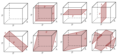
Figure 4: Counting GSD on $T^{2}_{o}$, that is $\text{Tr}_{{\cal H}_{T^{2}_{\text{o}}}}\,1$. The shaded 2-tori embedded into a $T^{3}$ represent Poincaré duals to elements of $H^{1}(M_{3},{\mathbb{Z}}_{2})\cong{\mathbb{Z}}_{2}^{3}$. The red letters A/P denote Anti-periodic/Periodic boundary conditions on the embedded 2-tori.

Similarly,

$$\text{Tr}_{{\cal H}_{T^{2}_{\text{o}}}}\,(-1)^{F}=Z(T^{2}_{\text{o}}\times S^{1}_{\text{P}})=\frac{1}{2}(1+7(-1)^{\nu})=\left\{\begin{array}[]{ll}-3,&\nu=1\mod 2\\ 4,&\nu=0\mod 2\end{array}\right.$$ (5.16)

which means that for $\nu=1\mod 2$ all states are femrionic. For the even spin structure on $T^{2}$ we have:

$$\text{Tr}_{{\cal H}_{T^{2}_{\text{e}}}}\,1=Z(T^{2}_{\text{e}}\times S^{1}_{\text{A}})=\frac{1}{2}(7+(-1)^{\nu})=\left\{\begin{array}[]{ll}3,&\nu=1\mod 2\\ 4,&\nu=0\mod 2\end{array}\right.$$ (5.17)

$$\text{Tr}_{{\cal H}_{T^{2}_{\text{e}}}}\,(-1)^{F}=Z(T^{2}_{\text{e}}\times S^{1}_{\text{P}})=\frac{1}{2}(7+(-1)^{\nu})=\left\{\begin{array}[]{ll}3,&\nu=1\mod 2\\ 4,&\nu=0\mod 2\end{array}\right..$$ (5.18)

So all states are bosonic. The result for all allowed spin structures, can be summarized as follows:

• For odd $\nu$: 3 fermionic states for ${T^{2}_{\text{o}}}$ and 3 bosonic states for ${T^{2}_{\text{e}}}$.

• For even $\nu$: 4 states, all bosonic, for both ${T^{2}_{\text{o}}}$ and ${T^{2}_{\text{e}}}$.

We can implement the similar counting for other 2+1D and 3+1D spin TQFTs given in [7]. Notice that at least for 2+1D fermionic topological orders/TQFTs up to some finite states of GSD were classified in [95]. Our GSD counting can be compared with [95].

So far we have focused on a 2+1D example, but more 2+1D/3+1D spin TQFT examples are given in Sec. 6.2 using the dimensional reduction scheme for GSD counting. We summarize these fermionic TQFTs and GSD data in Table 2.

6 Dimensional Reduction Scheme of Partition Functions and Topological Vacua

6.1 Bosonic Dimensional Reduction Scheme

Here we perform the dimensional reduction of TQFTs described in Sec. 2 for explicit bosonic examples, and match with data computed in Sec. 3 and 4. We write the decomposition in terms of eqn. (2.12), but applicable also to eqn. (2.1) and eqn. (2.2). The notation ${\cal C}^{d\mathrm{D}}$ below means a $d+1$D TQFTs.

For 3+1D ${{\mathbb{Z}}_{2}}$-gauge theory reduction to 2+1D, we can write the continuum field theory form

$${{\cal C}^{3\mathrm{D}}_{{\frac{2}{2\pi}}\int BdA}}=2{{\cal C}^{2\mathrm{D}}_{{\frac{2}{2\pi}}\int BdA}},\;\;\;\;\;$$ (6.1)

or equivalently in terms of the cocycle ${{\cal C}^{3\mathrm{D}}_{1}}=2{{\cal C}^{2\mathrm{D}}_{1}}$. The sub-index $1$ means a trivial cocycle. The $B$ fields represent a 2-form gauge field in ${\cal C}^{3\mathrm{D}}$, but represent a 1-form gauge field in ${\cal C}^{2\mathrm{D}}$. Here we take the compact $z$-direction (among the $x$-$y$-$z$-$t$ in 3+1D) as the compactification direction, and each sector comes from holonomy around the direction that is $\oint_{z}A=0$ or $\pi$ (in terms of the 1-cochain field $\oint_{z}a=0$ or $1$) respectively. The resulting sectors of 2+1D ${\mathbb{Z}}_{2}$ gauge theories are equivalent in this case. See Fig.3 for a physical illustration.

For 3+1D twisted ${({\mathbb{Z}}_{2})^{2}}$-gauge theory reduction to 2+1D, we obtain

$${{\cal C}^{3\mathrm{D}}_{\frac{2}{2\pi}\underset{i=1}{\overset{2}{\sum}}\int B_{i}dA_{i}+c_{122}A_{1}A_{2}dA_{2}}}={{\cal C}^{2\mathrm{D}}_{\frac{2}{2\pi}\int\underset{i=1}{\overset{2}{\sum}}B_{i}dA_{i}}}\oplus{{\cal C}^{2\mathrm{D}}_{\frac{2}{2\pi}\int(\underset{i=1}{\overset{2}{\sum}}B_{i}dA_{i}+A_{2}dA_{2})}}\oplus 2{{\cal C}^{2\mathrm{D}}_{\frac{2}{2\pi}\int(\underset{i=1}{\overset{2}{\sum}}B_{i}dA_{i}+A_{1}dA_{2})}}.\;\;\;\;\;$$ (6.2)

We can explain this easily by converting those continuous descriptions to the cochain-field theory description with 4-cocycle and 3-cocycles. Relevant cocycles are a 4-cocycle $\omega_{4,\text{II}}^{(12)}=(-1)^{\int{a_{1}\cup a_{2}\cup a_{2}\cup a_{2}}}$ in 3+1D; and also 3-cocycles 1, $\omega_{3,\text{I}}^{(1)}=(-1)^{\int{a_{1}\cup a_{1}\cup a_{1}}}\equiv(-1)^{\int(a_{1})^{3}}$ and $\omega_{3,\text{II}}^{(12)}=(-1)^{\int{a_{1}\cup a_{2}\cup a_{2}}}$ in 2+1D. Here all the $a_{i}$ (say $a_{1}$, $a_{2}$, etc.) are the ${\mathbb{Z}}_{2}$-valued 1-cochain field. In this section, all these $a_{i}$, $B$ and $A$ are dynamical fields, which we need to sum over all configurations in the path integral also in ${\cal C}^{d\mathrm{D}}$ to obtain long-ranged entangled TQFTs (instead of short-ranged entangled SPTs). The above eqn. (6.2) can be derived, effectively, as

$$\begin{split}{{\cal C}^{3\mathrm{D}}_{a_{1}\cup a_{2}\cup a_{2}\cup a_{2}}}&={{\cal C}^{2\mathrm{D}}_{1}}\oplus{{\cal C}^{2\mathrm{D}}_{(a_{2})^{3}}}\oplus{{\cal C}^{2\mathrm{D}}_{a_{1}\cup a_{2}\cup a_{2}}}\oplus{{\cal C}^{2\mathrm{D}}_{(a_{1}+a_{2})\cup a_{2}\cup a_{2}}}\\ &={{\cal C}^{2\mathrm{D}}_{1}}\oplus{{\cal C}^{2\mathrm{D}}_{(a_{2})^{3}}}\oplus 2{{\cal C}^{2\mathrm{D}}_{a_{1}\cup a_{2}\cup a_{2}}}.\end{split}$$ (6.3)

In the first line, we decompose the 3+1D theory with respect to holonomies around the compactifying $z$-direction (among the $x$-$y$-$z$-$t$ in 3+1D) which are $(\oint_{z}a_{1},\oint_{z}a_{2})=(0,0),(1,0),(0,1),(1,1)$. Then we obtain the second line by field redefinition, or equivalently a $\mathrm{SL}(2,\mathbb{Z}_{2})$ transformation, sending $a_{1}+a_{2}\to a_{1}$ in the last sector.

For 3+1D twisted ${({\mathbb{Z}}_{2})^{4}}$-gauge theory reduction to 2+1D, we can also use the cochain-field expression to ease the calculation,

$$\begin{split}{{\cal C}^{3\mathrm{D}}_{a_{1}\cup a_{2}\cup a_{3}\cup a_{4}}}&={{\cal C}^{2\mathrm{D}}_{1}}\oplus 4{{\cal C}^{2\mathrm{D}}_{a_{j}\cup a_{k}\cup a_{l}}}\oplus 6{{\cal C}^{2\mathrm{D}}_{{a_{j}\cup a_{k}\cup a_{l}}+{a_{j}\cup a_{k}\cup a_{l^{\prime}}}}}\\ &\;\;\;\;\;\;\oplus 4{{\cal C}^{2\mathrm{D}}_{{a_{j}\cup a_{k}\cup a_{l}}+{a_{j}\cup a_{k}\cup a_{m}}+{a_{j}\cup a_{l}\cup a_{m}}}}\oplus{{\cal C}^{2\mathrm{D}}_{{a_{1}\cup a_{2}\cup a_{3}}+{a_{1}\cup a_{2}\cup a_{4}}+{a_{1}\cup a_{3}\cup a_{4}}+{a_{2}\cup a_{3}\cup a_{4}}}}\\ &={{\cal C}^{2\mathrm{D}}_{1}}\oplus 10\;{{\cal C}^{2\mathrm{D}}_{a_{j}\cup a_{k}\cup a_{l}}}\oplus 5\;{{\cal C}^{2\mathrm{D}}_{{a_{1}\cup a_{2}\cup a_{3}}+{a_{1}\cup a_{2}\cup a_{4}}+{a_{1}\cup a_{3}\cup a_{4}}+{a_{2}\cup a_{3}\cup a_{4}}}}.\end{split}$$ (6.4)

In the first line, we get the each sector in the right hand side from the each holonomy $(\oint_{z}a_{1},\oint_{z}a_{2},\oint_{z}a_{3},\oint_{z}a_{4})\in\mathbb{Z}_{2}^{4}$ around the compactifying $z$-direction. We decompose the 16 sectors into a multiplet with multiplicities (1,4,6,4,1), where the first 1 selects $\vec{a}^{T}=(a_{1,z},a_{2,z},a_{3,z},a_{4,z})=(0,0,0,0)$; The second 4 selects only one element of $\vec{a}$ as 1 as nontrivial, given by the combinatory ${4\choose 1}=4$; The third 16 selects only two elements out of $\vec{a}$ as 1 as nontrivial, given by the combinatory ${4\choose 2}=6$; Similarly, the fourth ${4\choose 3}=4$ and the fifth ${4\choose 4}=1$ are selected. All these indices $j,k,l,l^{\prime},m$ given above are dummy but fixed and distinct indices, selected from the set $\{1,2,3,4\}$. In the second line of eqn. (6.4), it turns out that we can do a $M\in$ SL$(4,{\mathbb{Z}}_{2})$ transformation in the dimensional reduced sector, among the $\vec{a}^{T}=(a_{1},a_{2},a_{3},a_{4})$, to redefine the fields through $M\vec{a}=\vec{a}^{\prime}\to\vec{a}$. The second sector and third sector turn out to be the same, via a $M=M_{2\leftrightarrow 3}$. The fourth sector and fifth sector turn out to be the same, via a $M=M_{4\leftrightarrow 5}$.

$$M_{2\leftrightarrow 3}=\left(\begin{array}[]{cccc}1&1&0&0\\ 0&1&0&0\\ 0&0&1&0\\ 0&0&0&1\\ \end{array}\right),\;\;\;\;M_{4\leftrightarrow 5}=\left(\begin{array}[]{cccc}1&1&1&1\\ 0&1&0&0\\ 0&0&1&0\\ 0&0&0&1\\ \end{array}\right)\in\mathrm{SL}(4,{\mathbb{Z}}_{2}).$$

For example, we see $M_{23}$ can change ${(a_{1}+a_{2})\cup a_{3}\cup a_{4}}$ to ${a_{1}\cup a_{3}\cup a_{4}}$, thus we can combine the 6 of third sectors into the 4 of second sectors. Overall, similar forms of $M=M_{2\leftrightarrow 3}$ does the job to identify these 10 sectors as 10 equivalent copies of a TQFT written as $10\;{{\cal C}^{2\mathrm{D}}_{a_{j}\cup a_{k}\cup a_{l}}}$. Similarly, we can use the similar forms of $M=M_{4\leftrightarrow 5}$ to identify the last fourth and fifth sectors, obtaining 5 copies of a TQFT, written as $5\;{{\cal C}^{2\mathrm{D}}_{{a_{1}\cup a_{2}\cup a_{3}}+{a_{1}\cup a_{2}\cup a_{4}}+{a_{1}\cup a_{3}\cup a_{4}}+{a_{2}\cup a_{3}\cup a_{4}}}}$.

In terms of continuum gauge field theory, we can rewrite eqn. (6.4) as

$$\begin{split}&{{\cal C}^{3\mathrm{D}}_{\frac{2}{2\pi}\underset{i=1}{\overset{4}{\sum}}\int B_{i}dA_{i}+\frac{1}{\pi^{3}}A_{1}A_{2}A_{3}A_{4}}}={{\cal C}^{2\mathrm{D}}_{\frac{2}{2\pi}\underset{i=1}{\overset{4}{\sum}}\int B_{i}dA_{i}}}\\ &\;\;\;\;\oplus 10{{\cal C}^{2\mathrm{D}}_{\frac{2}{2\pi}\underset{i=1}{\overset{4}{\sum}}\int B_{i}dA_{i}+\frac{1}{\pi^{2}}A_{1}A_{2}A_{3}}}\oplus 5{{\cal C}^{2\mathrm{D}}_{\frac{2}{2\pi}\underset{i=1}{\overset{4}{\sum}}\int B_{i}dA_{i}+\frac{1}{\pi^{2}}(A_{1}A_{2}A_{3}+A_{1}A_{2}A_{4}+A_{1}A_{3}A_{4}+A_{2}A_{3}A_{4})}}.\end{split}$$ (6.5)

In terms of TQFT dimensional decomposition, eqn. (6.4)/eqn. (6.5) is the information we can obtain based on the field theory actions. What else topological data can we obtain to check the decompositions in eqn. (6.5)? We can consider:

1. GSD data on ${T^{3}}$ shows that

   $$\begin{split}&\text{GSD}_{T^{3},\;3+1\text{D-TQFT}}=\sum_{b}\text{GSD}_{T^{2},\;2+1\text{D-TQFT}^{\prime}(b)}\\ &\Rightarrow{\text{GSD}_{{T^{3}},\frac{2}{2\pi}\underset{i=1}{\overset{4}{\sum}}\int B_{i}dA_{i}+\frac{1}{\pi^{3}}A_{1}A_{2}A_{3}A_{4}}}=1576=256+15\times(2^{2}\times 22).\end{split}$$ (6.6)

   The GSD data only distinguish the $b=0$ trivial sector ${{\cal C}^{2\mathrm{D}}_{\frac{2}{2\pi}\underset{i=1}{\overset{4}{\sum}}\int B_{i}dA_{i}}}$ with GSD${}_{T^{2}}$=256 from the remaining 15 sectors. Each of the remaining 15 sectors has GSD $=88$, which is the same as the tensor product (${\mathbb{Z}}_{2}$ gauge theory) $\otimes$ (a non-Abelian $D_{4}$ gauge theory) with trivial DW cocycle in 2+1D [10]. Therefore, GSD cannot distinguish the second and the last sector of the decomposition eqn. (6.5).

2. GSD data on ${{\mathbb{RP}}^{3}}$ shows that

   $$\begin{split}{\text{GSD}_{{{\mathbb{RP}}^{3}},\frac{2}{2\pi}\underset{i=1}{\overset{4}{\sum}}\int B_{i}dA_{i}+\frac{1}{\pi^{3}}A_{1}A_{2}A_{3}A_{4}}}=11&=1\times 1+4\times{3\over 4}+6\times{3\over 4}+4\times{1\over 2}+1\times{1\over 2}.\\ &=1\times 1+10\times{3\over 4}+5\times{1\over 2}.\end{split}$$ (6.7)

   In this case, we first compute $Z({\mathbb{RP}}^{3}\times S^{1})=11$ for ${\frac{2}{2\pi}\underset{i=1}{\overset{4}{\sum}}\int B_{i}dA_{i}+\frac{1}{\pi^{3}}A_{1}A_{2}A_{3}A_{4}}$. This data matches with the dimensional reduced 16 sectors of 2+1D TQFTs in terms of their $Z({\mathbb{RP}}^{3})$ that we also compute. In terms of 2+1D TQFTs grouping in eqn. (6.4) as a multiplet (1,4,6,4,1), the first sector contributes $Z({\mathbb{RP}}^{3})=1$, each of the second (4) and third (6) contributes $Z({\mathbb{RP}}^{3})={3\over 4}$, and each of the fourth (4) and fifth (1) contributes $Z({\mathbb{RP}}^{3})={1\over 2}$.

3. We can also adopt additional data such as the modular ${\cal T}$ matrix of SL$(2,{\mathbb{Z}})$ representation, measuring the topological spin or the self-statistics of anyonic particle/string excitations, in [10]. The diagonal ${\cal T}$ matrix contains only four distinct eigenvalues, $(1,-1,i,-i)$. We can specify a ${\cal T}$ matrix by a tuple of numbers containing these eigenvalues, as $(N_{1},N_{-1},N_{i},N_{-i})$. We find

   $$\begin{split}{{\cal T}^{3D}_{\frac{2}{2\pi}\underset{i=1}{\overset{4}{\sum}}\int B_{i}dA_{i}+\frac{1}{\pi^{3}}A_{1}A_{2}A_{3}A_{4}}}&\text{in terms of }(N_{1},N_{-1},N_{i},N_{-i})=(836,580,80,80)\\ &=1\times(136,120,0,0)+10\times(48,32,4,4)+5\times(44,28,8,8).\end{split}$$ (6.8)

   The 10 sectors of ${\cal T}^{2D}$ with $(N_{1},N_{-1},N_{i},N_{-i})=(48,32,4,4)$ are again the same as ${\cal T}^{2D}$ of the (${\mathbb{Z}}_{2}$ gauge theory) $\otimes$ (a non-Abelian $D_{4}$ gauge theory) in 2+1D. The overall structure of ${\cal T}^{3D}$ decomposition agrees with $Z({\mathbb{RP}}^{3}\times S^{1})$ decomposition.

In summary, eqn. (6.5) suggest that there are at most three distinct classes among the 16 sectors of dimensional reduced 2+1D TQFTs, and the distinction among the three is guaranteed by the data of $Z({\mathbb{RP}}^{3})$ and ${\cal T}$ matrices.

For untwisted gauge theories, one can derive:

$${\cal C}^{3\mathrm{D}}_{\text{3+1D-${D_{4}}$ gauge}}=2{\cal C}^{2\mathrm{D}}_{\text{2+1D-${D_{4}}$ gauge}}\oplus 2{\cal C}^{2\mathrm{D}}_{\text{2+1D-$(Z_{2})^{2}$ gauge}}\oplus{\cal C}^{2\mathrm{D}}_{\text{2+1D-$Z_{4}$ gauge}},$$ (6.9)

$${\cal C}^{3\mathrm{D}}_{\text{3+1D-${Q_{8}}$ gauge}}=2{\cal C}^{2\mathrm{D}}_{\text{2+1D-${Q_{8}}$ gauge}}\oplus 3{\cal C}^{2\mathrm{D}}_{\text{2+1D-${Z_{4}}$ gauge}}.$$ (6.10)

Each conjugacy class of holonomy round the compactifying circle gives the lower dimensional theory with the maximal subgroup commuting with the holonomy as its subgroup. These results can be checked by the information of [10, 75] and our earlier section’s GSD data.

6.2 Fermionic Dimensional Reduction Scheme

Based on Sec. 2’s strategy, we examine the dimensional decomposition of some of the spin TQFTs listed in Sec. 5. We obtain these spin TQFTs from gauging some global symmetries of fermionic Symmetry-Protected Topological states (fSPTs).

6.2.1 2+1D $\rightarrow$ 1+1D gauged fSPT reduction: 2+1D ${\mathbb{Z}}_{2}^{2}\times{\mathbb{Z}}_{2}^{f}$ fSPT and its gauged spin-TQFT

Consider a 2+1D fSPT state with ${\mathbb{Z}}_{2}^{2}\times{\mathbb{Z}}_{2}^{f}$ symmetry and its partition function

$$Z_{\text{2+1D fSPT}}=e^{\frac{\pi}{2}i\int a_{1}\cup a_{2}\cup\tilde{\eta}}$$ (6.11)

where the precise definition of the action is spelled out in point 2) in the beginning of Sec. 5. When implementing the theory on a $M^{3}=M^{2}\times S^{1}$, depending on the spin structure and ${\mathbb{Z}}_{2}$ holonomies along $S^{1}$, it reduces to a 1+1D fSPT with ${\mathbb{Z}}_{2}^{2}\times{\mathbb{Z}}_{2}^{f}$ symmetry of one of the 3 following types:

1. Trivial.

   $$Z_{\text{1+1D fSPT}}=1.$$ (6.12)

   Gauged theory has GSD${}^{\text{I}}=4b$ (given by the partition function of $M^{2}=S^{1}\times S^{1}$) independently on the spin structure on $S^{1}$.

2. $$Z_{\text{1+1D fSPT}}=e^{\pi i\int(\sum_{i,j=1}^{2}\epsilon_{ij}\alpha_{i}\,a_{j})\cup\eta}.$$ (6.13)

   Where $\alpha_{i}\in{\mathbb{Z}}_{2}$ are some parameters not all simultaneously zero, $a_{i}\in H^{1}(M^{2},{\mathbb{Z}}_{2})$ describe background ${\mathbb{Z}}_{2}$ gauge fields and $\epsilon_{ij}$ is the standard anti-symmetric tensor. The formal expression for the action has the following definition:

   $$\int_{M^{2}}a\cup\eta\equiv\eta[\text{PD}(a)]\equiv\left\{\begin{array}[]{cc}1,&\text{odd spin structure on PD}[a],\\ 0,&\text{even spin structure on PD}[a].\end{array}\right.$$ (6.14)

   where the spin-structure on 1-manifold $\text{PD}[a]$ is induced from the spin structure on $M^{2}$ in on obvious way (cf. beginning of Sec. 5). Note that

   $$\int_{M^{2}}(a_{1}+a_{2})\cup\eta=\int_{M^{2}}a_{1}\cup\eta+\int_{M^{2}}a_{2}\cup\eta+\int_{M^{2}}a_{1}\cup a_{2}.$$ (6.16)

   The gauged theory has GSD${}^{\text{II}}_{\text{P}}=2\times(1f+0b)$ for the odd spin structure on $S^{1}$ and GSD${}^{\text{II}}_{\text{A}}=2\times(0f+1b)$ for the even spin structure on $S^{1}$.

3. $$Z_{\text{1+1D fSPT}}=e^{\pi i\int a_{1}\cup a_{2}+(\sum_{i,j=1}^{2}\epsilon_{ij}\alpha_{i}\,a_{j})\cup\eta}.$$ (6.17)

   Gauged theory, for any $\alpha_{i}$, has GSD${}^{\text{III}}=1b$ independently on the spin structure on $S^{1}$.

Namely, for the even spin strucutre and trivial ${\mathbb{Z}}_{2}$ holonomies along $S^{1}$, the 2+1D fSPT reduces to trivial (type I) theory on $M^{2}$. For the odd spin strucutre and non-trivial ${\mathbb{Z}}_{2}$ holonomies, it reduces to a theory of type II with $\alpha_{i}=\int_{S^{1}}a_{i}$. For the odd spin strucutre and trivial ${\mathbb{Z}}_{2}$ holonomies along $S^{1}$, or the even spin strucure and non-trivial ${\mathbb{Z}}_{2}$ holonomies, it reduces to a theory of type III with $\alpha_{i}=\int_{S^{1}}a_{i}$.

Consider now the gauged 2+1D fSPT on $M^{3}=T^{3}$. Let us order the circles in $T^{3}$ such that the first one is the time circle and the last one is the $S^{1}$ on which we are doing reduction. The GSD decomposition then reads as follows:

$$\begin{array}[]{c}\text{GSD}_{\text{PP}}=\text{GSD}_{\text{P}}^{\text{III}}+3\,\text{GSD}_{\text{P}}^{\text{II}}=1b+3\times 2\times(1f+0b)=6f+1b,\\ \text{GSD}_{\text{AP}}=\text{GSD}_{\text{A}}^{\text{III}}+3\,\text{GSD}_{\text{A}}^{\text{II}}=1b+3\times 2\times(0f+1b)=7b,\\ \text{GSD}_{\text{PA}}=\text{GSD}_{\text{P}}^{\text{I}}+3\,\text{GSD}_{\text{P}}^{\text{III}}=4b+3\times 1b=7b,\\ \text{GSD}_{\text{AA}}=\text{GSD}_{\text{A}}^{\text{I}}+3\,\text{GSD}_{\text{A}}^{\text{III}}=4b+3\times 1b=7b.\end{array}$$ (6.18)

The decompositions of GSDs can be promoted to the decomposition of the spin-TQFT functor. For odd spin structure on $S^{1}$:

$${\cal C}^{\text{2D}}_{\frac{\pi}{2}\int a_{1}\cup a_{2}\cup\tilde{\eta}}={\cal C}^{\text{1D}}_{\pi\int a_{1}\cup a_{2}}\oplus{\cal C}^{\text{1D}}_{\pi\int a_{1}\cup\eta}\oplus{\cal C}^{\text{1D}}_{\pi\int a_{2}\cup\eta}\oplus{\cal C}^{\text{1D}}_{\pi\int(a_{1}+a_{2})\cup\eta}=\\ {\cal C}^{\text{1D}}_{\pi\int a_{1}\cup a_{2}}\oplus 3{\cal C}^{\text{1D}}_{\pi\int a_{1}\cup\eta},$$ (6.19)

For even spin structure on $S^{1}$:

$${\cal C}^{\text{2D}}_{\frac{\pi}{2}\int a_{1}\cup a_{2}\cup\tilde{\eta}}={\cal C}^{\text{1D}}_{0}\oplus{\cal C}^{\text{1D}}_{\pi\int a_{1}\cup a_{2}+a_{1}\cup\eta}\oplus{\cal C}^{\text{1D}}_{\pi\int a_{1}\cup a_{2}+a_{2}\cup\eta}\oplus{\cal C}^{\text{1D}}_{\pi\int a_{1}\cup a_{2}+(a_{1}+a_{2})\cup\eta}=\\ {\cal C}^{\text{1D}}_{0}\oplus 3{\cal C}^{\text{1D}}_{\pi\int a_{1}\cup a_{2}+a_{1}\cup\eta},$$ (6.20)

where we used field redefinitions to combine equivalent theories together. Note that all the summands except the first one give isomorphic Hilbert spaces on $S^{1}$. This is the reason for the factors of 3 in (6.18).

6.2.2 3+1D $\rightarrow$ 2+1D gauged fSPT reduction: 3+1D ${\mathbb{Z}}_{4}^{2}\times{\mathbb{Z}}_{2}^{f}$ fSPT and its gauged spin-TQFT

Consider a 3+1D fSPT state with ${\mathbb{Z}}_{4}^{2}\times{\mathbb{Z}}_{2}^{f}$ symmetry and its partition function

$$Z_{\text{3+1D fSPT}}=e^{\pi\int(a_{1}\mod 2)\cup(a_{2}\mod 2)\cup\text{Arf}}$$ (6.21)

where the precise definition of the action is spelled out in point 4) in the beginning of Sec. 5. When putting on $M^{4}=M^{3}\times S^{1}$, depending on the spin structure and ${\mathbb{Z}}_{2}$ holonomies along $S^{1}$, it reduces to a 2+1D fSPT with ${\mathbb{Z}}_{4}^{2}\times{\mathbb{Z}}_{2}^{f}$ symmetry of one of the 3 following types:

1. Trivial.

   $$Z_{\text{2+1D fSPT}}=1.$$ (6.22)

   Gauged theory has GSD${}^{\text{I}}=256b$ independently on spin structure on $T^{2}$.

2. $$Z_{\text{2+1D fSPT}}=e^{\pi i\int(\sum_{i,j}^{2}\epsilon_{ij}\alpha_{i}\,a_{j}\mod 2)\cup\text{Arf}}.$$ (6.23)

   Where $\alpha_{i}\in{\mathbb{Z}}_{2}$ are some parameters not all simultaneously zero and $a_{i}\mod 2\in H^{1}(M^{3},{\mathbb{Z}}_{2})$ describes background ${\mathbb{Z}}_{2}$ gauge fields. Gauged theory has GSD${}^{\text{II}}_{\text{PP}}=16\times 12f$ for the odd spin structure on $T^{2}$ and $\text{GSD}^{\text{II}}_{\text{PA}}=\text{GSD}^{\text{II}}_{\text{AP}}=\text{GSD}^{\text{II}}_{\text{AA}}=16\times 12b$ for an even spin structure on $T^{2}$.

3. $$Z_{\text{2+1D fSPT}}=e^{\pi i\int(\sum_{i,j}^{2}\epsilon_{ij}\alpha_{i}\,a_{j}\mod 2)\cup\text{Arf}+(a_{1}\mod 2)\cup(a_{2}\mod 2)\cup\eta}$$ (6.24)

   where $\alpha_{i}\in{\mathbb{Z}}_{2}$ are not all simultaneously zero. Gauged theory, for any $\alpha_{i}$, has GSD${}^{\text{III}}=16\times 9b$ independently on spin structure on $T^{2}$. Note that from the definition eqn. (5.5), we derive

   $$\int_{M^{3}}(b_{1}+b_{2})\cup\text{Arf}=\int_{M^{3}}b_{1}\cup\text{Arf}+\int_{M^{3}}b_{2}\cup\text{Arf}+\int_{M^{3}}b_{1}\cup b_{2}\cup\eta.$$ (6.25)

4. $$Z_{\text{2+1D fSPT}}=e^{\pi i\int(a_{1}\mod 2)\cup(a_{2}\mod 2)\cup\eta}.$$ (6.26)

   Gauged theory has GSD${}^{\text{IV}}_{\text{PP}}=16\times(6f+1b)$ for the odd spin structure on $T^{2}$ and $\text{GSD}^{\text{IV}}_{\text{PA}}=\text{GSD}^{\text{IV}}_{\text{AP}}=\text{GSD}^{\text{IV}}_{\text{AA}}=16\times 7b$ for an even spin structure on $T^{2}$.

As for 2+1D $\rightarrow$ 1+1D reduction, for the even spin strucutre on $S^{1}$ and trivial mod 2 holonomies along $S^{1}$, the 3+1D fSPT reduces to trivial (type I) theory on $M^{3}$. For the odd spin strucutre and non-trivial mod 2 holonomies it reduces to a theory of type II with $\alpha_{i}=\int_{S^{1}}a_{i}\mod 2$. For the odd spin strucutre and trivial mod 2 holonomies along $S^{1}$ it reduces to the type IV theory. For the even spin strucure and non-trivial mod 2 holonomies, it reduces to a theory of type III with $\alpha_{i}=\int_{S^{1}}a_{i}\mod 2$.

Consider now 3+1D fSPTs on $M^{4}=T^{4}$. Let us again order the circles in $T^{4}$ such that the first one is the time circle and the last one is the $S^{1}$ on which we are doing reduction. The GSD decomposition than reads as follows:

$$\begin{array}[]{c}\text{GSD}_{\text{(odd)P}}=4\text{GSD}_{\text{(odd)}}^{\text{IV}}+12\,\text{GSD}_{\text{(odd)}}^{\text{II}}=4\times 16\times(6f+1b)+12\times 16\times 12f=64\times(42f+1b),\\ \text{GSD}_{\text{(even)P}}=4\text{GSD}_{\text{(even)}}^{\text{IV}}+12\,\text{GSD}_{\text{(even)}}^{\text{II}}=4\times 16\times 7b+12\times 16\times 12b=64\times 43b,\\ \text{GSD}_{\text{(odd)A}}=4\text{GSD}_{\text{(odd)}}^{\text{I}}+12\,\text{GSD}_{\text{(odd)}}^{\text{III}}=4\times 16\times 16b+12\times 16\times 9b=64\times 43b,\\ \text{GSD}_{\text{(even)A}}=4\text{GSD}_{\text{(even)}}^{\text{I}}+12\,\text{GSD}_{\text{(even)}}^{\text{III}}=4\times 16\times 16b+12\times 16\times 9b=64\times 43b.\\ \end{array}$$ (6.27)

where (odd) denotes even PP spin structure on $T^{2}$ and (even) denotes any of the even spin structures, PA, AP or AA, on $T^{2}$.

The decompositions of GSDs can be promoted to the decomposition of the spin-TQFT functor. For odd spin structure on $S^{1}$:

$${\cal C}^{\text{3D}}_{\pi\int(a_{1}\mod 2)\cup(a_{2}\mod 2)\cup\text{Arf}}=4{\cal C}^{\text{2D}}_{\pi\int(a_{1}\mod 2)\cup(a_{1}\mod 2)\cup\eta}\oplus 12{\cal C}^{\text{2D}}_{\pi\int(a_{1}\mod 2)\cup\text{Arf}}$$ (6.28)

For even spin structure on $S^{1}$:

$${\cal C}^{\text{3D}}_{\pi\int(a_{1}\mod 2)\cup(a_{2}\mod 2)\cup\text{Arf}}=4{\cal C}^{\text{2D}}_{0}\oplus 12{\cal C}^{\text{2D}}_{\pi\int(a_{1}\mod 2)\cup\text{Arf}+(a_{2}\mod 2)\cup\text{Arf}}$$ (6.29)

We used field redefinitions to identify equivalent theories. Note that all the summands except the first one give isomorphic Hilbert spaces on $T^{2}$. This is the reason for the factors of 7 in (6.27).

This dimension decomposition method can be applied to all examples given in Table 2.

7 Long-Range Entangled Bulk/Boundary Coupled TQFTs

Now we consider bulk/boundary coupled TQFT system. In the work of Ref. [26], for a given bulk $d+1$ dimensional $G$-symmetry protected phase characterized by a Dijkgraaf-Witten (DW) cocycle $\omega^{d+1}\in{\cal H}^{d+1}(BG,{U(1)})$, a $d$D boundary $K$-gauge theory coupled with the $d+1$D bulk SPT is constructed via a so-called the group extension or symmetry extension scheme. The groups $G$ and $K$ form an exact sequence

$$1\to K\to H\stackrel{{\scriptstyle r}}{{\to}}G\to 1,$$

such that $r^{*}\omega^{d+1}=1\in{\cal H}^{d+1}(BH,{U}(1))$ where $r^{*}$ is the pullback of the homomorphism $r$. The $r$ is a surjective group homomorphism. The $H$ is a total group associated to the boundary. To help the readers to remember the group structure assignment to the bulk/boundary, we can abbreviate the above group extension as,

$$1\to K_{\text{boundary}}\to H_{\text{boundary}}\stackrel{{\scriptstyle r}}{{\to}}G_{\text{bulk}}\to 1.$$ (7.1)

This structure is used throughout Sec. 7. In Appendix of [26], some examples of GSDs are computed for both bulk SRE (ungauged) case and bulk LRE (dynamically gauged) case, based on the explicit lattice spacetime path integral. Here we examine some examples exposed there, and will argue that when bulk is gauged, some of the boundary degrees of freedom “dissolve” into the bulk. In other words, we will show that after gauging the whole system, a certain group-extension construction in eqn. (7.1) is actually equivalent (dual or indistinguishable) to a group-breaking construction also explained in Ref. [26] associated to an inclusion $\iota$:

$$G^{\prime}_{\text{boundary}}\stackrel{{\scriptstyle\iota}}{{\to}}G_{\text{bulk}}.$$ (7.2)

where $G^{\prime}$ is a subgroup that $G$ breaks to, and the inclusion should satisfy $\iota^{*}\omega^{d+1}=1\in{\cal H}^{d+1}(BG^{\prime},{U}(1))$ where $\iota^{*}$ is its pullback. The annotations below $G^{\prime}$ and $G$ indicate site/link variables are valued in those groups in boundary and bulk respectively as was the case of eqn. (7.1).

A heuristic reasoning is the following. This is a generalization of the statement of [97, 98] that a 1+1D gauge theory, with an abelian finite gauge group $K$ but without Dijkgraaf-Witten cocycle twist, has a global symmetry group isomorphic to $K$, and when the global $K$ is further gauged, the resulting theory is trivial [97, 98]. In the setup given by eqn. (7.1), the $K$ gauge theory on the boundary is coupled with anomalous $G$-symmetry. Gauging the bulk $G$ symmetry reduces the boundary degrees of freedom as in the pure 1+1D set up. When $K$ is small enough, the boundary degrees of freedom can even be completely gauged away, and no boundary degrees of freedom remain. Before gauging, the bulk $G$ symmetry have the $G$-preserving boundary condition and coupled with the boundary degrees of freedom. However, when the boundary $K$-gauge theory is gauged away by gauging the bulk $G$, the whole bulk/boundary coupled system should be equivalent to just bulk $G$ symmetry with some boundary condition without being coupled with 1+1D system, possibly accompanied by a decoupled 1+1D system on the boundary. Namely, we stress the following:
There is an equivalence, only after gauging, between “a certain bulk/boundary coupled system” and “the bulk system with only some boundary conditions.”
For such a system to be consistent, the boundary condition should break $G$ into some non-anomalous subgroup $G^{\prime}$. This discussion is summarized in Figure 5.

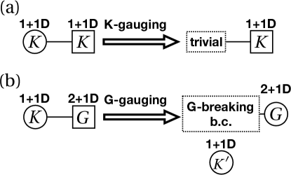
Figure 5: (a) The “re-gauging” of a 1+1D (or 2d) abelian finite $K$-gauge theory [97, 98]. In general, a group surrounded by a circle means a gauged symmetry, and a group surrounded by a square means a global symmetry. There is a global non-anomalous $K$ group acting on the theory faithfully, which is shown by the $K$ surrounded by a square. When $K$ is gauged, the whole system becomes trivial, meaning the Hilbert space is 1-dimensional on any topology. (b) This case is what we focus on in Sec. 7.1. We start from 1+1D $K$ gauge theory coupled with anomalous $G$ symmetry. The anomalous symmetry is thought to be realized as an SPT phase in 2+1D. After gauging the bulk $G$-symmetry, resulting system would be equivalent to a 2+1D $G$-theory with some boundary condition breaking $G$ into a subgroup $G^{\prime}$ and without coupling with a 1+1D system. There can possibly be a decoupled $K^{\prime}$ gauge theory on the boundary. In the examples, however, we may neglect $K^{\prime}$ as absence.

In the rest of this section, we show how the above scenario occurs in more detail in two examples, in Sec. 7.1 and Sec. 7.2. We will then compute partition functions on the $I^{1}\times S^{1}$ topology in two ways: using the explicit lattice path-integral model coming from [26]’s eqn. (7.1) and using the non-trivial boundary condition on $G$ with no boundary degrees of freedom. Furthermore, we will try to generalize the discussion to 3+1D/2+1D system, in Sec. 7.3. However, we will see that a certain exotic type of boundary condition of the bulk theory occurs after the bulk gauging. The complete understanding of the higher dimensional case remained for a future work.

We clarify that in the discussions of Sec. 7, when we state “breaking” this means breaking the (gauge/global) symmetry with respect to the electric sector (instead of the magnetic sector), and when we state “preserving” this means preserving the (gauge/global) symmetry with respect to the electric sector (instead of the magnetic sector), too.

We will also use the language of [26] summarized in Table 3 throughout Sec. 7.

System	$d+1$D Bulk/ $d$D Boundary Entanglement property;	Group Extension Construction
System (i)	SRE/SRE SPT/Symmetry	$1\to K_{\text{boundary}}^{\text{global sym}}\to H_{\text{boundary}}^{\text{global sym}}\stackrel{{\scriptstyle r}}{{\to}}G_{\text{bulk}}^{\text{global sym}}\to 1$
System (ii)	SRE/LRE SPT/SET(TQFT)	$1\to K_{\text{boundary}}^{\text{gauge}}\to H_{\text{boundary}}^{\text{total}}\stackrel{{\scriptstyle r}}{{\to}}G_{\text{bulk}}^{\text{global sym}}\to 1$
System (iii)	LRE/LRE TQFT/TQFT	$1\to K_{\text{boundary}}^{\text{gauge}}\to H_{\text{boundary}}^{\text{gauge}}\stackrel{{\scriptstyle r}}{{\to}}G_{\text{bulk}}^{\text{gauge}}\to 1$

Table 3: We re-examine the $d+1$D Bulk/ $d$D Boundary coupled system based on a group extenssion construction, developed in [26], in terms of more field theoretic understandings in Sec. 7. The system we analyze the most is System (iii)’s LRE/LRE Bulk/Boundary TQFT. LRE/SRE stands for Long/Short Ranged Entangled. SPT/SET stands Symmetry Protected/Enriched Topological states. We will especially comment about the gauging process (say, from System (i) to (ii), or (ii) to (iii)), and especially focus on the issue still left open: The boundary conditions and some of their dualities to breaking construction eqn. (7.2), after gauging $G_{\text{bulk}}$.

7.1 2+1/1+1D LRE/LRE TQFTs: Gauging an extension construction is dual to a gauge-breaking construction

Let us start from the easiest case as a warm up, where the bulk is a 2+1D $G=\mathbb{Z}_{2}$ gauge theory. Namely, the bulk is the $\mathbb{Z}_{2}$ gauge theory of field $A$ (represented by a ${\mathbb{Z}}_{2}$-valued 1-cochain) with the unique non-trivial cocycle $(-1)^{\int A\cup A\cup A}$. This cocycle can be cancelled by a boundary cochain when the boundary has a $K=\mathbb{Z}_{2}$ gauge theory, as shown in [26]. In this case the sequence eqn. (7.1) is

$$1\to{\mathbb{Z}_{2}^{K}}_{\text{boundary}}\to{\mathbb{Z}_{4}^{H}}_{\text{boundary}}\to{\mathbb{Z}_{2}^{G}}_{\text{bulk}}\to 1.$$ (7.3)

We use the upper indices $G$ to denote the group for the bulk, and the indices $K$ and $H$ to denote the groups for the boundaries following eqn. (7.1) and [26]. In [26], the GSD on $D^{2}$ is computed to be $Z(D^{2}\times S^{1})=1$ when both bulk and boundary are dynamical. This hints that the boundary $\mathbb{Z}_{2}^{K}$ degrees of freedom are actually absent when the bulk $\mathbb{Z}_{2}^{G}$ is gauged. Below we aim to show that, only after gauging $\mathbb{Z}_{2}^{G}$, this extension construction eqn. (7.3) becomes equivalent to the breaking construction eqn. (7.2) (also formulated in [26]) as

$$1_{\text{boundary}}^{G^{\prime}}\to{\mathbb{Z}_{2}^{G}}_{\text{bulk}}.$$ (7.4)

We use the upper indices $G^{\prime}$ to denote the preserved group for the boundary as eqn. (7.2).

In brief, it can be explained as follows. On boundary, there is a vortex operator $\phi(x)$ localized at a point $x$. For the boundary $\mathbb{Z}_{2}^{K}$ gauge theory to be coupled with the bulk $\mathbb{Z}_{2}^{G}$ symmetry, the operator should be shifted under the bulk $\mathbb{Z}_{2}$ transformation: $\phi\to\phi+\lambda,$ where $\lambda$ is a $\mathbb{Z}_{2}$ valued parameter of the bulk symmetry transformation. Then, we have an operator invariant under the bulk $\mathbb{Z}_{2}$ transformation

$$\exp(\mathrm{i}\pi(\int_{x_{1}}^{x_{2}}A-\phi(x_{1})+\phi(x_{2}))),$$ (7.5)

where $A$ is the bulk $\mathbb{Z}_{2}^{G}$ field, $x_{1}$ and $x_{2}$ are the boundary points. When the bulk $\mathbb{Z}_{2}^{G}$ is gauged, the boundary vortex operator $\phi$ is gauged out and therefore there is no longer a $\mathbb{Z}_{2}^{K}$ degeneracy on boundary, and the bulk electric electric $\mathbb{Z}_{2}$ Wilson line can end on the boundary. Thus, the whole system is indistinguishable to just a bulk $\mathbb{Z}_{2}^{G}$ gauge theory with boundary condition breaking the electric $\mathbb{Z}_{2}^{G}$, without any additional degrees of freedom on the boundary.

We give a more explicit explanation in the following. Before gauging the bulk $\mathbb{Z}_{2}^{G}$, the partition function of the full spacetime, with bulk ${M^{3}}$ of 2+1D $\mathbb{Z}_{2}^{G}$-SPTs and boundary $({\partial M})^{2}$ of 1+1D $\mathbb{Z}_{2}^{K}$-gauge theory, is

$$Z_{A}=(-1)^{\int_{M^{3}}A\cup A\cup A}\sum_{{\alpha\in C^{1}((\partial M)^{2},{\mathbb{Z}}_{2}),}\atop{\phi\in C^{0}((\partial M)^{2},{\mathbb{Z}}_{2})}}(-1)^{\int_{\partial M}\phi\delta\alpha+\alpha\cup A+\phi A\cup A},$$ (7.6)

where $\phi$ and $\alpha$ are ${\mathbb{Z}}_{2}$-valued 0-cochain and 1-cochain fields respectively. We denote all such ${\mathbb{Z}}_{n}$ valued $m$-cochain fields on the spacetime manifold ${\cal M}$ in the cochain $C^{m}({\cal M},{\mathbb{Z}}_{n})$. The $Z_{A}$ depends on the background $\mathbb{Z}_{2}^{G}$ field $A$, and only $\phi$ and $\alpha$ are dynamical here. Under their gauge transformations, $A\to A+\delta\lambda$, $\phi\to\phi+\lambda$ and $\alpha\to\alpha+\lambda\delta\lambda$ with $\lambda$ is an integral 0-cochain ($\lambda\in C^{0}(M,{\mathbb{Z}}_{2})$), similar to the gauge-invariant calculation done in [77], we find the $Z_{A}$ is gauge invariant.

After gauging the bulk $\mathbb{Z}_{2}^{G}$, we propose the partition function of the full spacetime, with bulk ${M^{3}}$ of 2+1D $\mathbb{Z}_{2}^{G}$-gauge theory with boundary (of 1+1D $\mathbb{Z}_{4}^{H}$-gauge theory including also $\mathbb{Z}_{2}^{K}$ gauge sector), in continuum field description, is

$$Z={\cal N}^{-1}\sum_{A}Z_{A}=\int[DA][DB][D\phi]\;e^{i(\frac{1}{2\pi}\int\limits_{M^{3}}(2BdA+AdA)+\frac{1}{2\pi}\int\limits_{\partial M}(2\phi dB+2BA+\phi dA))}.$$ (7.7)

Here we use continuum field notations, where $A$ and $B$ are 1-form gauge fields, and $\phi$ becomes a 0-form scalar. The whole partition function $Z$ is gauge invariant, under $A\to A+d\eta_{A}$, $B\to B+d\eta_{B}$ and $\phi\to\phi-\eta_{A}$, where $\eta_{A}$/$\eta_{B}$ are locally 0-forms. The $\alpha$ as a 1-cochain field in eqn. (7.6) is related to the B as the continuum 1-form field in eqn. (7.7). We give several remarks in order to explain the gauging $\mathbb{Z}_{2}^{G}$ process:

1. SRE/SRE bulk/boundary: Starting from System (i) SRE/SRE bulk/boundary in Table 3, as shown in [26], this is a $\mathbb{Z}_{2}^{G}$-SPTs in a bulk, while it has a $\mathbb{Z}_{4}^{H}$-symmetry extended boundary. All global symmetries are preserved and unbroken.

2. SRE/LRE bulk/boundary $\Rightarrow$ SRE/(SRE+LRO) bulk/boundary: After gauging the ${\mathbb{Z}}_{2}^{K}$ on the boundary, we arrive System (ii)’s SRE/LRE bulk/boundary in Table 3, whose partition function is $Z_{A}$ in eqn. (7.6). In Sec. 3.3 of Ref. [26], it is found that the two holonomies of ${\mathbb{Z}}_{2}^{K}$ (or two ground states on a disk $D^{2}$ for this System (ii)) has different ${\mathbb{Z}}_{2}^{G}$-symmetry charge. The trivial holonomy of ${\mathbb{Z}}_{2}^{K}$ has a trivial (no or even) ${\mathbb{Z}}_{2}^{G}$ charge. The non-trivial holonomy of ${\mathbb{Z}}_{2}^{K}$ has an odd ${\mathbb{Z}}_{2}^{G}$ charge. We find this fact can be understood as eqn. (7.6)’s $Z_{A}$ has the ${\mathbb{Z}}_{2}^{K}$-holonomy $\int\alpha$ coupled to the ${\mathbb{Z}}_{2}^{G}$-background field in $(-1)^{\int_{\partial M}\alpha\cup A}$. Such a ${\mathbb{Z}}_{2}^{K}$-gauge theory turns out to develop ${\mathbb{Z}}_{2}^{G}$-spontaneous global symmetry breaking (SSB) long-range order (LRO) [26]. Thus, it turns out that this SRE/LRE bulk/boundary by design turns into an SRE/SRE bulk/boundary, because the ${\mathbb{Z}}_{2}^{G}$-SSB boundary has a gapped edge, which has LRO (but no Goldstone modes) but is SRE.

3. LRE/LRE bulk/boundary: After gauging the ${\mathbb{Z}}_{2}^{G}$ in the bulk (the boundary ${\mathbb{Z}}_{2}^{K}$ is also gauged), we arrive System (iii)’s LRE/LRE bulk/boundary in Table 3, whose partition function we propose as $Z$ in eqn. (7.7). By massaging eqn. (7.7), we obtain

   $$Z=\int[DA][DB][D\phi]\;e^{i(\frac{2}{2\pi}\int\limits_{M^{3}}(A+d\phi)dB+\frac{1}{2\pi}\int\limits_{M^{3}}(A+d\phi)d(A+d\phi))}.$$ (7.8)

   From this expression of the partition function we can make several physical observations and predictions listed in below.

   (1). When we gauge bulk’s ${\mathbb{Z}}_{2}^{G}$, both $A$, $\phi$ and $\alpha$ (cochain fields of eqn. (7.6)) become dynamical. This yields $A+\delta\phi$ having no gauge transformation on the boundary, thus $B$ integration implies

   $$(A+\delta\phi)|_{\partial M}=0.$$ (7.9)

   The dynamical vortex field $\phi$ (at the open ends of $A$) becomes deconfined on the boundary. This can be viewed as the ${\mathbb{Z}}_{2}$ electric charge particle (the $e$ anyon) becomes deconfined and condensed on the boundary. By anyon condensed on the boundary, we mean that there can be nontrivial expectation value

   $$\langle\exp(i\phi)\rangle\neq 0,$$ (7.10)

   for the ground state(s), since the $\phi$ are freely popped up and absorbed into the boundary. Thus, gauging bulk’s ${\mathbb{Z}}_{2}^{G}$ causes however the $\mathbb{Z}_{2}^{G}$ gauge symmetry broken on the boundary.

   (2) We can (and later will) also read the boundary condition directly from the cochain fields in eqn. (7.6). The ${\mathbb{Z}}_{2}^{G}$-SPT partition function indicates the following boundary condition after gauging ${\mathbb{Z}}_{2}^{G}$:

   $${A|_{\partial M}=0,\;\;\;A\cup A|_{\partial M}=0},$$

   in terms of cohomology. For example, integrating out $\alpha$ in eqn. (7.6) forces $A$ to be exact on the boundary. The first condition is equivalent to eqn. (7.9), while the second condition automatically holds at the path integral after imposing the first condition.

   (3). After gauging $\mathbb{Z}_{2}^{G}$, we expect all boundary operators can be dissolved into the bulk. Which means the apparent boundary operator $(-1)^{\int_{C}\alpha},$ where $C$ is a 1-cycle in $\partial M$, should be identified with the magnetic $\mathbb{Z}_{2}^{G}$ line operator in the bulk, since the electric $\mathbb{Z}_{2}^{G}$ is broken on the boundary as we saw. Thus we can physically understand the conversion from ${\int\alpha}$ (1-cochain field) to ${\int B}$ (1-form magnetic ${\mathbb{Z}}_{2}$ field), from eqn. (7.6)’s $Z_{A}$ to eqn. (7.7)’s $Z$, only after gauging the $\mathbb{Z}_{2}^{G}$. This agrees with the fact that the GSD is $Z(D^{2}\times S^{1})=1$ in [26].

   (4). As an additional check, we consider GSD on $I^{1}\times S^{1}$. From [26], the lattice computation shows $Z(I^{1}\times T^{2})=2$. This is consistent with the alternative description of the symmetry breaking boundary condition, since the $\int A$ line can have a nontrivial $\mathbb{Z}_{2}$ value along the interval $I^{1}$, while cannot have nontrivial holonomy along the spatial $S^{1}$. (This coincides with the gauge symmetry breaking boundary condition explored in [19], e.g. Table II). See also Table 4

LRE/LRE 2+1D bulk/1+1D boundary coupled TQFTs
$Z(M^{2}\times S^{1})$	$Z(T^{3})$	$Z(D^{2}\times S^{1})$	$Z(I^{1}\times T^{2})$
spatial topology	$T^{2}$	$D^{2}$	$I^{1}\times S^{1}$
GSD	4	1	2

Table 4: The GSDs of the LRE/LRE bulk/boundary TQFT theory of dynamically gauged $(-1)^{\int A\cup A\cup A}$ SPT. The boundary theory is constructed via eqn. (7.3) in [26]. Our Sec. 7.1 can explain the GSD data in terms of field theoretic description.

In summary, the LRE/LRE bulk-boundary coupled TQFT systems given by the exact sequence eqn. (7.3), only when $\mathbb{Z}_{2}^{G}$ is gauged, is equivalent to just $\mathbb{Z}_{2}^{G}$ breaking boundary condition, namely, the double semion condensation (see [19]), when both bulk and boundary groups are gauged. The gauge symmetry breaking condition is given in [26] eqn. (7.4) as $1\to\mathbb{Z}_{2}^{G}.$ In 2+1D/1+1D LRE/LRE bulk/boundary, the underlying physics of eqn. (7.3) and eqn. (7.4) coincides with the double semion condensation. For example, we can write the bulk gauge theory as a twisted ${\mathbb{Z}}_{2}$ gauge theory or ${\mathbb{Z}}_{2}$ double-semion topological order, ${\int\frac{2}{2\pi}BdA}+\frac{1}{2\pi}AdA,$ then the double semion condensation can be achieved by $\left.A\right|_{\partial M}=0$ boundary condition in eqn. (7.9). We can gap the boundary by turning on the cosine sine-Gordon term

$$g\int dtdx\cos(2\phi)$$ (7.11)

at a strong coupling $g$, where the scalar field $\phi(x,t)$ is the same vortex operator mentioned above. Under SL$(2,{\mathbb{Z}})$ field redefinition, we can rewrite the bulk theory as ${\int\frac{1}{4\pi}\Big{(}\begin{smallmatrix}2&0\\ 0&-2\end{smallmatrix}}\Big{)}_{IJ}\,A_{I}^{\prime}dA_{J}^{\prime},$ then we can gap the boundary by the cosine term of vortex field $\phi^{\prime}_{I}$ of $A_{I}^{\prime}$, [19]

$$g\int dtdx\cos(2(\phi^{\prime}_{1}+\phi^{\prime}_{2}))$$ (7.12)

at a strong coupling $g$. See the comparison of the physical setup of double semion condensation, or precisely the condensation of semion $s$ and anti-semion $\bar{s}$ in [19].

7.2 2+1/1+1D LRE/LRE TQFTs: Gauging an extension construction is dual to a partially gauge-breaking construction

We would like to generalize the argument in the previous subsection into a more nontrivial case, namely 2+1/1+1D coupled system associated to the following exact sequence:

$$1\to(\mathbb{Z}_{2})^{K}_{\text{boundary}}\to(D_{4}\times\mathbb{Z}_{2})^{H}_{\text{boundary}}\to(\mathbb{Z}_{2}^{3})^{G}_{\text{bulk}}\to 1,$$ (7.13)

where the leftmost $(\mathbb{Z}_{2})^{K}$ goes into the order-8 non-Abelian dihedral group $D_{4}$, and the $\mathbb{Z}_{2}$ in the middle just become one of the factors of $(\mathbb{Z}^{3}_{2})^{G}$. Again the upper index $G$ denotes the group for the bulk, and the indices $K$ and $H$ denote the groups for the boundaries following eqn. (7.1) and [26]. The bulk $\mathbb{Z}^{3}_{2}$ gauge fields $A_{1},A_{2},A_{3}$ have the exponentiated action

$$(-1)^{\int_{M}A_{1}\cup A_{2}\cup A_{3}}.$$ (7.14)

To cancel the anomaly induced by the bulk, the boundary dynamical $\mathbb{Z}_{2}$ cochain fields $\alpha$ and $\phi$ have the coupling

$$Z_{A}=(-1)^{\int_{M}A_{1}\cup A_{2}\cup A_{3}}\sum_{{\alpha\in C^{1}((\partial M)^{2},{\mathbb{Z}}_{2}),}\atop{\phi\in C^{0}((\partial M)^{2},{\mathbb{Z}}_{2})}}(-1)^{\int_{{\partial}M}(\phi\delta\alpha+\alpha\cup A_{1}+\phi A_{2}\cup A_{3})}.$$ (7.15)

This indicates the boundary conditions

$$A_{1}=0,\quad A_{2}\cup A_{3}=0,$$ (7.16)

for the LRE/LRE system.

Let us compute the partition function on $I^{1}\times T^{2}$ with the boundary condition eqn. (7.16), and compare it with the result from the method of the Appendix of [26]. To be precise, the boundary condition “$A_{1}=0$” means that the field $A_{1}$ is an element of the relative cohomology $H^{1}(M,\partial M;\mathbb{Z}_{2})$, while keeping $A_{2,3}$ to be inside $H^{1}(M;\mathbb{Z}_{2})$. The second condition of eqn. (7.16) will be imposed by the path-integral, as we will see. Then, the partition function is

$$Z(I^{1}\times T^{2})={\cal N}^{-1}\sum_{A}Z_{A}={\cal N}^{-1}\sum_{(A_{1},A_{2},A_{3})}(-1)^{\int_{I\times T^{2}}A_{1}\cup A_{2}\cup A_{3}},$$ (7.17)

where $(A_{1},A_{2},A_{3})$ runs through $H^{1}(M,\partial M;\mathbb{Z}_{2})\oplus H^{1}(M;\mathbb{Z}_{2})^{\oplus 2}$ with $M=I\times T^{2}$ as said, and ${\cal N}$ is a normalization constant which is to be determined. Note that $A_{1}\cup A_{2}\cup A_{3}$ defines an element of $H^{3}(M,\partial M)$ so that it can be integrated over the fundamental class $[M]\in H_{3}(M,\partial M)$. In this expression, only the first condition of eqn. (7.16) is imposed by hand, while the summation over $A_{1}$ with the sign acts as a projection (times an integer) imposing the second condition.

Let us first compute the partition function eqn. (7.17) up to the normalization constant ${\cal N}$. It is convenient to pack the holonomy data $(A_{1},A_{2},A_{3})$ into a $3\times 3$ matrix

$$H_{ij}=\int_{\text{$i$-th direction}}A_{j}\in\mathbb{Z}_{2},$$ (7.18)

where the first direction is $I^{1}$ and the second and third directions are $S^{1}$’s in $T^{2}$ of $M=I^{1}\times T^{2}$. The partition function up to the normalization constant can be computed by

$${\cal N}Z(I^{1}\times T^{2})=\sum_{H}(-1)^{\mathrm{det}H}=20,$$ (7.19)

where the summation is constrained by the conditions $A_{1}\in H^{1}(M,\partial M;\mathbb{Z}_{2})$ and $A_{2},A_{3}\in H^{1}(M;\mathbb{Z}_{2})^{\oplus 2}$, which mean $H_{21}=H_{31}=H_{12}=H_{13}=0$. In the sum of eqn. (7.19), contribution from the configurations which do not satisfy the second equation of eqn. (7.16) on boundary is automatically canceled. For example, take a configuration given by

$$H=\begin{pmatrix}H_{11}&0&0\\ 0&1&0\\ 0&0&1\end{pmatrix}.$$ (7.20)

With this configuration, $\int_{T^{2}}A_{2}\cup A_{3}=1$ which does not satisfy the second equation of eqn. (7.16). However, summation over $H_{11}$ yeilds

$$\sum_{H_{11}=0,1}(-1)^{\mathrm{det}\,\mathrm{diag}(H_{11},1,1)}=0.$$ (7.21)

In this way, the summation over $H_{11}$ in eqn. (7.19) is essentially just projecting out the configurations which does not satisfy the second equation of eqn. (7.16), and therefore the partition function $Z$ counts the number of configurations satisfying eqn. (7.16) up to some constant.

The normalization constant ${\cal N}$ should be the number of residual gauge transformations which fixes the cohomology classes $(A_{1},A_{2},A_{3})$. Such gauge transformations are given by elements of $H^{0}(M,\partial M;\mathbb{Z}_{2})\oplus H^{0}(M;\mathbb{Z}_{2})^{\oplus 2}=\mathbb{Z}_{2}^{\oplus 2}$, therefore the normalization constant ${\cal N}$ is $4$. Then, the partition function can be computed to be

$$Z(I^{1}\times T^{2})=5.$$ (7.22)

Our independent computation matches exactly with the lattice model computation [26] based on the exact sequence eqn. (7.13), see Table 5.

LRE/LRE 2+1D bulk/1+1D boundary coupled TQFTs
$Z(M^{2}\times S^{1})$	$Z(T^{3})$	$Z(D^{2}\times S^{1})$	$Z(I^{1}\times T^{2})$
spatial topology	$T^{2}$	$D^{2}$	$I^{1}\times T^{1}$
GSD	22	1	5

Table 5: The GSDs of the LRE TQFT theory of dynamically gauged eqn. (7.14). The boundary theory is constructed via eqn. (7.13). Our Sec. 7.2 can explain the GSD data in terms of field theoretic description.

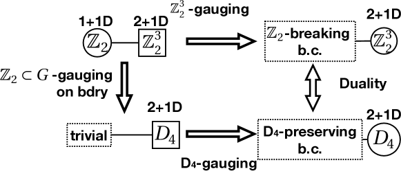
Figure 6: The interpretation of the boundary condition eqn. (7.16). The downward arrow is due to [98]. The boundary condition eqn. (7.16) breaks one of $\mathbb{Z}_{2}\subset(\mathbb{Z}_{2}^{3})^{G}$, and preserves (the electric parts of) the other two. On the other hand, we can do the same gauging in two steps. First we gauge one $\mathbb{Z}_{2}$ only on boundary, getting the trivial theory coupled with non-anomalous $D_{4}$, and then we gauge every symmetry realized in the system. In this way, we get $D_{4}$ gauge theory in the bulk with $D_{4}$ preserving boundary condition, which should be dual to the twisted $(\mathbb{Z}_{2}^{3})^{G}$ gauge theory in the bulk with ${\mathbb{Z}}_{2}$-breaking boundary condition.

The $\mathbb{Z}_{2}^{3}$ gauge theory with the action is known to be equivalent to the $D_{4}$ gauge theory (the order 8 dihedral group)[39]. The boundary condition eqn. (7.16) can be understood as the $D_{4}$ preserving boundary condition. Then, the partition function $Z(I^{1}\times T^{2})=5$ exactly counts the number of $D_{4}$ holonomies up to conjugacy around the $S^{1}$ inside a time slice $I^{1}\times S^{1}$. This observation is in line with a result in [98]. In [98], it was shown that when a $\mathbb{Z}_{2}$ subgroup of $\mathbb{Z}_{2}^{3}$ symmetry with anomaly eqn. (7.14) of a 1+1D theory is dynamically gauged, the resulting theory has a non-anomalous $D_{4}$ symmetry. We can divide the bulk $(\mathbb{Z}_{2}^{3})^{G}$ gauging into two parts, as depicted in Fig. 6, one is gauging of the $\mathbb{Z}_{2}$ subgroup on boundary, and the other is gauging of the rest of the symmetry. When the first $\mathbb{Z}_{2}\in G$ global symmetry is gauged on boundary, the $\mathbb{Z}_{2}^{K}$ gauge theory on the boundary is gauged away, and the resulting system is the trivial theory coupled with non-anomalous $D_{4}$ symmetry due to the result of [98]. Then, gauging the rest of the global symmetry merely results in the bulk $D_{4}$ gauge theory with $D_{4}$ preserving boundary condition. This is consistent with the fact that the $D_{4}$ gauge theory in $2+1$D is dual to the twisted $\mathbb{Z}_{2}^{3}$ gauge theory[39]. See also Figure 6.

In summary, the group extension construction eqn. (7.13) of coupled bulk/boundary (after gauging $G$) system is equivalent/dual to the partially gauge breaking construction as eqn. (7.2) into

$$(\mathbb{Z}_{2}^{2})^{G^{\prime}}_{\text{boundary}}\to(\mathbb{Z}_{2}^{3})^{G}_{\text{bulk}}.$$ (7.23)

7.3 3+1/2+1D LRE/LRE TQFTs: Comment on constructions of gauging an extension, and 1-form breaking v.s. “fuzzy-composite” breaking

The system described by the action eqn. (7.15) can be generalized to $3+1$D $\mathbb{Z}_{2}^{4}$ gauge theory whose exponentiated action is

$$(-1)^{\int A_{1}\cup A_{2}\cup A_{3}\cup A_{4}}$$ (7.24)

where $(A_{1},A_{2},A_{3},A_{4})\in H^{1}(M;\mathbb{Z}_{4})^{\oplus 4}$ are $\mathbb{Z}_{2}^{4}$ cocycle fields. Correspondingly, we consider the following new exact sequence, following eqn. (7.1):

$$1\to(\mathbb{Z}_{2})^{K}_{\text{boundary}}\to(D_{4}\times\mathbb{Z}_{2}^{2})^{H}_{\text{boundary}}\to(\mathbb{Z}_{2}^{4})^{G}_{\text{bulk}}\to 1,$$ (7.25)

with an order-8 non-Abelian dihedral group $D_{4}$. Namely, the anomaly described by eqn. (7.24) can be cancelled by a $\mathbb{Z}_{2}^{K}$ gauge theory on a 2+1D boundary. GSDs of this bulk-boundary coupled system when both bulk and boundary are gauged for some topologies, computed by the lattice model described in [26], now we compute the new data and list it in Table 6.

LRE/LRE 3+1D bulk/2+1D boundary coupled TQFTs
$Z(M^{3}\times S^{1})$	$Z(T^{4})$	$Z(D^{3}\times S^{1})$	$Z(D^{2}\times T^{2})$	$Z(I^{1}\times T^{3})$
spatial topology	$T^{3}$	$D^{3}$	$D^{2}\times S^{1}$	$I^{1}\times T^{2}$
GSD	1576	1	50	484

Table 6: The GSDs of the LRE TQFT theory of dynamically gauged eqn. (7.24) on spatial topologies $M_{\text{time slice}}^{3}$, which are equal to partition functions $Z(M^{3}\times S^{1})$, computed by lattice path integral construction [26]. On each boundary of $M_{\text{time slice}}^{3}$, there is a $\mathbb{Z}_{2}^{K}$ gauge theory and coupled with the bulk through the exact sequence eqn. (7.25) via $1\to\mathbb{Z}_{2}^{K}\to(D_{4}\times\mathbb{Z}_{2}^{2})^{H}\to(\mathbb{Z}_{2}^{4})^{G}\to 1$. Here both the bulk/boundary are LRE/LRE coupled TQFTs. Our Sec. 7.3 can explain the GSD data in terms of field theoretic description.

For the boundary $\mathbb{Z}_{2}^{K}$ gauge theory to cancel the anomaly eqn. (7.24), there should be the following coupling:

$$(-1)^{\int_{\partial M}(\alpha\cup A_{1}\cup A_{2}+\beta\cup A_{3}\cup A_{4})},$$ (7.26)

where $\alpha$ is the boundary $\mathbb{Z}_{2}$ gauge field, $\beta$ is its magnetic dual. Integrating $\alpha$ and $\beta$ out, we get the following boundary conditions

$$A_{1}\cup A_{2}=0,\quad A_{3}\cup A_{4}=0.$$ (7.27)

The partition function on $M$ with this boundary condition would be counted by

$$Z(M)={\cal N}(M)\sum_{(A_{1},A_{2},A_{3},A_{4})}(-1)^{\int_{M}{A_{1}\cup A_{2}\cup A_{3}\cup A_{4}}}$$ (7.28)

where summation should be taken over some cohomology group which precisely realizes the boundary condition implicated by eqn. (7.27), and ${\cal N}(M)$ is the normalization factor counting the residual gauge transformations. Unfortunately, the precise cohomology group which actually realize the above condition is harder to determine. We don’t have an exact answer for ${\cal N}(M)$ yet. Nonetheless, we can at least count the possible $\mathbb{Z}_{2}^{4}$ holonomies consistent with eqn. (7.27).

For $M=I^{1}\times T^{2}\times S^{1}$, we can parametrize possible holonomies by a 3 by 4 matrix

$$H_{ij}=\int_{S_{i}^{1}}A_{j}\in\mathbb{Z}_{2},$$ (7.29)

where $S_{i}^{1}$ is the $i$th 1-cycle of $T^{3}$. We define 2 by 2 submatrices $H(a,b;c,d)$ of $H$ by taking $a$th and $b$th rows and $c$th and $d$th columns of $H$. The boundary condition eqn. (7.27) forces that

$$\mathrm{Det}(H(a,b;c,d))=0$$ (7.30)

for $(c,d)=(1,2)$ or $(c,d)=(3,4)$. The number of matrices $H$ with elements $0$ or $1$ satisfying eqn. (7.30) is 484. Since we are yet to determine the physics affected by the $I^{1}$ direction and the normalization constant ${\cal N}(M)$, this is not a complete computation. However, the fact that the number of possible holonomies around $T^{3}$ with the condition eqn. (7.27) coincides with the GSD computed by the lattice computation, it suggest that the condition eqn. (7.27) is physically sensible in some way. Similarly, for the topology $M=D^{2}\times T^{2}$, we can count the holonomies around $T^{2}$ satisfying eqn. (7.27) to be 100, which is different from $Z(D^{2}\times T^{2})$ calculated by the lattice model by a factor of two, which is controlled by ${\cal N}(M)$.

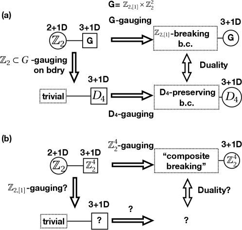
Figure 7: (a) A straightforward generalization of Figure 6. In one higher dimension, one $\mathbb{Z}_{2}$ of $(\mathbb{Z}_{2}^{3})^{G}$ in 2+1D/1+1D case is replaced by higher form $\mathbb{Z}_{2}$ symmetry here in 3+1D/2+1D, see eqn. (7.33). (b) Currently we do not know precisely how to generalize from the previous Fig. 6 associated to eqn. 7.13 to the present case associated to eqn. (7.25). A possible relationship with the case of (a) is discussed in the main text. The downord arrow should be $\mathbb{Z}_{2,[1]}$-gauging on the boundary in some sense to get a trivial theory out of the $\mathbb{Z}_{2}$ gauge theory in 2+1D, but the precise relation of $\mathbb{Z}_{2,[1]}$ to the $(\mathbb{Z}_{2}^{4})^{G}$ is left open for future investigation.

Mysteriously the situation here is not an obvious generalization of what was studied in the previous section. Rather, a straightforward generalization of the situation eqn. (7.13) is that the bulk theory has a $\mathbb{Z}_{2,[1]}\times\mathbb{Z}_{2}^{2}$ symmetry, where $\mathbb{Z}_{2,[1]}$ is a 1-form $\mathbb{Z}_{2}$ symmetry, with an action

$$(-1)^{\int_{M^{4}}A^{(2)}\cup A_{3}\cup A_{4}},$$ (7.31)

where $A^{(2)}$ is the 2-form gauge field of $\mathbb{Z}_{2,[1]}$ symmetry and $a_{1,2}$ are 1-form gauge fields of $\mathbb{Z}_{2}^{2}$. See Figure 7(a). A boundary $\mathbb{Z}_{2}$ gauge field $\alpha$ can be coupled with the field $A^{(2)}$ through

$$(-1)^{\int_{\partial M}\alpha\cup A^{(2)}+\beta\cup A_{3}\cup A_{4}}.$$ (7.32)

The recent paper [99] shows that when $\mathbb{Z}_{2,[1]}$ of $\mathbb{Z}_{2,[1]}\times(\mathbb{Z}_{2}^{2})^{G}$ with an anomaly eqn. (7.31) is gauged in 2+1D, the resulting theory has a non-anomalous $D_{4}$ symmetry. Therefore the whole picture of Figure 6 can be lifted in this case, by lifting one $\mathbb{Z}_{2}$ symmetry into $\mathbb{Z}_{2,[1]}$. In particular, a breaking boundary condition

$$\mathbb{Z}_{2}^{2}\to\mathbb{Z}_{2,[1]}\times(\mathbb{Z}_{2}^{2})^{G}$$ (7.33)

should be dual to the $D_{4}$ preserving boundary condition.

What was studied in this subsection is more involved. Instead of eqn. (7.32), we have the coupling eqn. (7.26). Still, we can observe a similarity between the eqn. (7.26) and eqn. (7.32). Namely, $A_{1}\cup A_{2}$ plays the roll of $A^{(2)}$ in eqn. (7.32). Thus, one might somehow find relations between these $\mathbb{Z}_{2}^{2}$ fields and a “composite” $\mathbb{Z}_{2,[1]}$ field. One might regard the boundary condition eqn. (7.27) relating to a boundary condition breaking this “composite” $\mathbb{Z}_{2,[1]}$. See Figure 7(b).

The boundary condition eqn. (7.27) suggests that, on the boundary, some composite strings, composed of particles charged under the $(\mathbb{Z}_{2}^{4})^{G}$ symmetries, are condensed, and thus this boundary condition might have some novel feature. Since the dimensionality of the composite strings (1+1D) and their composed particles (0+1D) is different, here we introduce the new concept of the “fuzzy composite object” composed by one-lower-dimensional object. We add fuzzy to emphasize the dimensionality differences between the two objects. The condensation of such “fuzzy composite objects” on the boundary can be understood as the “fuzzy composite-breaking” boundary condition.

Investigating this boundary condition in detail, in particular constructing a microscopic model (other than the lattice Hamiltonian and lattice path integral given in Ref. [26]) to realize the physical mechanism at the microscopic level on the lattice will be interesting.

8 Conclusions

Below we conclude with remarks on long-range entanglements and entanglement entropy, the generalization of topological boundary conditions, and the potential application to strongly-coupled gauge theories, and quantum cosmology.

8.1 Remarks on Long-Range Entanglement and Entanglement Entropy with Topological Boundaries

It is well known that the long range entanglement (LRE) can be partially captured by the topological entanglement entropy (TEE) [100, 101]. In 2+1D, the topological entanglement entropy is the constant part of the entanglement entropy (EE), and one can extract the TEE by computing a linear combination of entanglement entropy as suggested[100, 101]. For discrete gauge theories with gauge group $G$, when the entanglement cut does not wrap around the spatial cycle, the topological entanglement entropy is $-\log|G|$. For instance, the $(\mathbb{Z}_{N})^{k}$ gauge theory has the TEE $=-k\log n$. Notice that the value of the TEE is independent of the twisting parameter (i.e. cocycle) of twisted gauge theories, hence one is not likely to distinguish different Dijkgraaf-Witten (DW) theories with the same gauge group using the TEE of the ground state wavefunctions on a closed manifold.

In the following, we consider two generalizations to obtain a richer structure of the entanglement entropy.

One generalization is to go to 3+1 dimensions and consider the Walker-Wang twisted theory. As was discussed in [102] and [56], for discrete gauge theories of Walker-Wang type [103] with gauge group $\mathbb{Z}_{N}$ and twisting parameter $p$ (namely, $\int BF+BB$ in Sec. 3.3), the topological entanglement entropy across a torus (which does not wrap around the spatial cycle) is $-\log\gcd(N,2p)$, which depends on the twisting parameter. Hence the TEE can probe the twisting level $p$ of Walker-Wang model. This fact can be understood as follows: The genuine line and surface operators of the Walker-Wang model coincide with the line and surface operators of ${\mathbb{Z}}_{\gcd(n,2p)}$ gauge theory, see [35] and Sec. 3.3. The TEE of the $\mathbb{Z}_{N}$ Walker-Wang model with twists is precisely the TEE of the $\mathbb{Z}_{\gcd(N,2p)}$ ordinary gauge theory without twists, i.e. $-\log|G_{\text{eff}}|=-\log\gcd(N,2p)$.

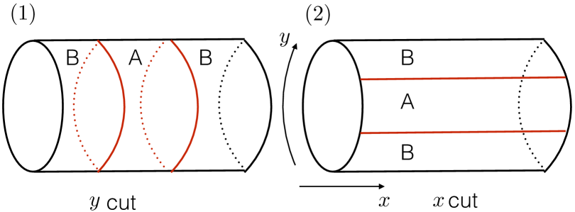
Figure 8: In the left panel, the entanglement cuts wrap around the $y$-cycle, which we denote the $y$-cut. In the right panel, the entanglement cuts extend along $x$ direction, and end at the two boundaries, which we denote the $x$-cut.

Another generalization is to consider the entanglement entropy on a spatial manifold with boundaries where the entanglement cut wraps around spatial cycles. We consider the $\mathbb{Z}_{2}$ gauge theories (i.e., ${\mathbb{Z}}_{2}$-toric code model and ${\mathbb{Z}}_{2}$-double semion [a twisted $\mathbb{Z}_{2}$] model) on a cylinder geometry with two boundaries, as shown in Fig. 8. Let us first focus on the left panel and discuss the ${\mathbb{Z}}_{2}$-toric code model. In the toric code model, there are four types of anyons $\{1,e,m,\epsilon\}$. Let us denote $|W_{x},T_{x}\rangle$ to be the eigenstate of the line operators $W_{x}=e^{i\oint_{x}A_{x}dx}$ (i.e., $e$-line in the $x$ direction) and $T_{x}=e^{i\oint_{x}B_{x}dx}$ (i.e., $m$-line in the $x$ direction). A generic ground state is a linear combination of $|W_{x},T_{x}\rangle$,

$$|\psi\rangle=c_{1}|1\rangle+c_{e}|e\rangle+c_{m}|m\rangle+c_{\epsilon}|\epsilon\rangle$$ (8.1)

where we label $|1\rangle\equiv|0,0\rangle,|e\rangle=|1,0\rangle,|m\rangle=|0,1\rangle,|\epsilon\rangle=|1,1\rangle$, and the coefficients are properly normalized $|c_{1}|^{2}+|c_{e}|^{2}+|c_{m}|^{2}+|c_{\epsilon}|^{2}=1$. Following the computation in [104], we can derive that the entanglement entropy of $|\psi\rangle$ is a linear combination of the entanglement entropy of $|1\rangle,|e\rangle,|m\rangle,|\epsilon\rangle$, denoted as $S^{y}(|\psi\rangle)=-\sum_{i=1,e,m,\epsilon}|c_{i}|^{2}\log|c_{i}|^{2}+\sum_{i=1,e,m,\epsilon}|c_{i}|^{2}S^{y}(|i\rangle)$ where the super-script $y$ indicates the direction of the entanglement cut. In the following, we are only interested in the subleading (topological) part of the entanglement entropy, i.e.,

$$S^{y}_{\mathrm{topo}}(|\psi\rangle)=-\sum_{i=1,e,m,\epsilon}|c_{i}|^{2}\log|c_{i}|^{2}+\sum_{i=1,e,m,\epsilon}|c_{i}|^{2}S^{y}_{\mathrm{topo}}(|i\rangle)$$ (8.2)

Because $e$ and $m$ are both self and mutual bosons, they can separately condense on the boundaries. Let us denote $a|b$ as $a$-condensation on the left boundary and $b$-condensation on the right boundary. There are 3 types of boundary conditions on a cylinder: the $e|e$, $m|m$ and $e|m$. When both boundaries are $e$-condensation, i.e, the $e|e$ boundary condition, there are two distinct sectors, with odd/even number of $e$-lines across the entanglement cut respectively. The generic ground state is

$$|\psi,e|e\rangle=c_{1}|1\rangle+c_{e}|e\rangle$$ (8.3)

where we have explicitly shown the boundary condition. Notice that there are no $|m\rangle$ and $|\epsilon\rangle$ in the expansion because the $m$-particle and $\epsilon$-particle cannot end on the boundary. Therefore the $m$-line and the $\epsilon$-line must cross the entanglement cut twice. For each sector, the even/odd-ness of the $e$-line crossing the entanglement cut is fixed, hence $S^{y}_{\mathrm{topo}}(|1\rangle)=S^{y}_{\mathrm{topo}}(|e\rangle)=-\log 2$. According to Eq. (8.2), we have

$$\begin{split}S^{y}_{\mathrm{topo}}(|\psi,e|e\rangle)&=-|c_{1}|^{2}\log|c_{1}|^{2}-|c_{e}|^{2}\log|c_{e}|^{2}-\log 2\\ &=-|c_{1}|^{2}\log|c_{1}|^{2}-(1-|c_{1}|^{2})\log(1-|c_{1}|^{2})-\log 2\end{split}$$ (8.4)

When $|c_{1}|^{2}=|c_{e}|^{2}=\frac{1}{2}$, the entanglement entropy $S^{y}_{\mathrm{topo}}(|\psi,e|e\rangle)$ is maximized, $S^{y}_{\mathrm{MaxES},\mathrm{topo}}(|\psi,e|e\rangle)=0$. When $|c_{1}|^{2}=0,|c_{e}|^{2}=1$ or $|c_{1}|^{2}=1,|c_{e}|^{2}=0$, the entanglement entropy is minimized, $S^{y}_{\mathrm{MinES},\mathrm{topo}}(|\psi,e|e\rangle)=-\log 2$. We can further consider other boundary conditions and the entanglement cuts along the $x$ direction, and the results are summarized in Table 7(a). Furthermore, we also consider the entanglement entropy of the double semion model as shown in Table 7(b). In the double semion model, there are four types of anyons $\{1,s,\bar{s},b\}$, where the only nontrivial boson is $b$. Hence there is only one type of boundary condition, i.e., $b$ condensation on both boundaries, which we denote as $b|b$. From the data in Table 7(a) and 7(b), we have the following observations:

(a) b.c $e|e$ $m|m$ $e|m$ $S_{\mathrm{MaxES}}^{y}$ 0 0 $-\log 2$ $S_{\mathrm{MinES}}^{y}$ $-\log 2$ $-\log 2$ $-\log 2$ $S_{\mathrm{MaxES}}^{x}$ 0 0 $0$ $S_{\mathrm{MinES}}^{x}$ $-\log 2$ $-\log 2$ $0$           (b) b.c $b|b$ $S_{\mathrm{MaxES}}^{y}$ 0 $S_{\mathrm{MinES}}^{y}$ $-\log 2$ $S_{\mathrm{MaxES}}^{x}$ 0 $S_{\mathrm{MinES}}^{x}$ $-\log 2$

Table 7: (a) Maximal and minimal entanglement entropy of the ${\mathbb{Z}}_{2}$-toric code associated with various boundary conditions. (b) Maximal and minimal entanglement entropy of the ${\mathbb{Z}}_{2}$-double semion model associated with various boundary conditions.

1. The maximal and minimal entanglement entropy depend on the boundary condition. In particular, when the types of boundary conditions are the same, $S_{\mathrm{MaxES}}-S_{\mathrm{MinES}}=\log 2$. However, when the types of boundary conditions are different, $S_{\mathrm{MaxES}}-S_{\mathrm{MinES}}=0$.

2. When the types of boundary conditions differ on two sides, the entanglement entropy is sensitive to whether the cut is in the $x$-direction or the $y$-direction. This enables us to use the entanglement entropy to probe the boundary conditions.

We can implement the above approach to other examples studied in Sec. 7. In particular, given a bulk LRE system, we can design various boundary conditions (by group extension or by 0-form/higher-form breaking) on different boundaries. By generalizing the above analysis, we expect that EE is sensitive to not only the bulk but also the boundary/interface conditions. We leave a systematic analysis of the interplay between other boundary/interface conditions and the long range entanglement for future work.

8.2 More Remarks

1. Counting extended (line/surface) operators: For 3+1D bosonic Abelian-$G$ TQFTs (with or without cocycle twists) we studied, the number of distinct types of pure line operators (viewed as the worldline of particle excitations) and the number of distinct types of pure surface operators (viewed as the worldsheet of string/loop excitations) are the same, equal to the number of group elements in $G$ (thus the order of group $|G|$). By a pure surface operator, we mean that the particular surface operator does not have additional lower dimensional line operators attached; and vice versa. In a spacetime picture, a pure surface operator is associated to the worldsheet of pure string/loop excitations (of a constant time slice) that does not have additional particles attached. For 3+1D bosonic non-Abelian-$G$ TQFTs, with or without cocycle twists, we however expect that the number of distinct line/surface operators is related to the number of representation/conjugacy classes of $G$. In both case, we find that the number of pure line and pure surface operators are equivalent. One simple argument [44, 81] is that the number of ground states on the spatial manifold $S^{2}\times S^{1}$ in the Hilbert space must be spanned by (1) the eigenstates obtained from inserting all possible pure line operators along $S^{1}$ into $D^{3}\times S^{1}$ or (2) the eigenstates obtained from inserting all possible pure surface operators along $S^{2}$ into $S^{2}\times D^{2}$, because TQFT assigns a state-vector in a Hilbert space to an open manifold, in the spacetime path integral picture. Here we use the fact that $\partial(D^{3}\times S^{1})=\partial(S^{2}\times D^{2})=S^{2}\times S^{1}$ and the gluing along their boundary produces $(D^{3}\times S^{1})\sqcup(S^{2}\times D^{2})=S^{4}$ [44]. It is obviously that the operators along $S^{1}$ must be 1-lines, and the operators along $S^{2}$ must be 2-surfaces where the loop excitations created by this surface can be shrunk to nothing into the vacuum. Thus, they correspond to pure line/surface operators creating pure particle/string excitations. Because the GSD on $S^{2}\times S^{1}$ from two derivations is the same, the numbers of linear-independent pure line operators equal that of pure surface operators.

   For fermionic spin-TQFTs (with or without twists from gauging the cobordism topological terms), the line/surface operators in general will have additional labels compared to the bosonic case. In particular, for line operators, one can introduce a 0+1D fermionic SPT (labelled by ${\mathbb{Z}}_{2}$) supported on the line operator. Note that, as often required in QFT, the line operators should be equipped with framing (trivialization of the normal bundle) in order to be well defined. Then, the spin structure on the spacetime manifold induces a spin structure on the support of the line operator. For a non-trivial choice (i.e. $1\in{\mathbb{Z}}_{2}$) of the 0+1D SPT, the expectation value of the line operator will be multiplied by $\pm 1$ for even/odd induced spin structure. As in the bosonic case, the surface operators can be understood in terms of drilling out a tabular neighborhood of the operator and considering the theory on the resulting manifold with boundary with some condition on the holonomies on the boundary. For fermionic theories, one has to also choose a spin-structure on this manifold with boundary. This choice corresponds to the extra label assigned to the surface operator.

2. Fuzzy-composite object/breaking and extended operators: Earlier in Introduction eqn. (1.9) and in Sec. 7.3’s eqn. (7.27), we introduce a new mechanism to obtain a peculiar gapped topological boundary condition: $\left.{A_{i}\cup A_{j}}\right|_{\Sigma^{3}}=0$ that could be viewed as the condensation of a fuzzy-composite string formed by two different particles (associated to the ends of two different line operators). We term it as the condensation of the fuzzy-composite object associated to the open ends of a set of extended operators. More generally, we could anticipate that in higher spacetime dimensions, say ${M^{d+1}}$, there could be other general topological boundary conditions on ${\Sigma^{d}}=\partial{M^{d+1}}$ as

   $$\left.{A_{i}\cup A_{j}}\cup B_{k}\cup\dots\right|_{\Sigma^{d}}=0,$$ (8.6)

   in terms of the condensation of the composite object from a set of extended operators of different dimensionality (1-form, 2-form fields, etc., or 1-cochain, 2-cochain fields, etc.). Its further detailed study is left for the future.

3. Boundary/Interface Deconfinement: We had discussed in Sec. 7 (See also [26]), gauging dynamically the bulk of SRE/LRE Bulk/Boundary coupled TQFTs to obtain the LRE/LRE Bulk/Boundary coupled TQFTs in Sec. 7. We notice that the former system has a SRE bulk (e.g. SPT state) thus naturally has only non-fractionalized excitations in the bulk. The later system has a LRE bulk (e.g. topologically ordered state) thus can have also deconfined fractionalized excitations even in the bulk. However, we stress that the important ingredient, for both cases, is that the deconfined fractionalized excitations happen on the boundary/interface, without much energy penalty. In Sec. 7, we find that the deconfined fractionalized excitations indeed condense on the boundary/interface. On the lattice scale, the energy cost for having deconfined excitations in the SRE bulk is $\Delta E\to\infty$ (i.e. impossible), while that in the LRE bulk costs only $\Delta E\simeq\#J$ (some order of lattice coupling $J$, see Fig. 1). But having deconfined excitations on the boundary/interface is $\Delta E\simeq 0$, if the ground state is obtained from extended operators ending on the boundary.

   We note that there are some recent interests to study the deconfined domain walls [107, 108, 109] (See also footnote 33, and Reference therein [105]), where the bulks of systems are however confined without fractionalized excitations but only the boundary harbors deconfined excitations. Our work potentially could help to understand such systems systematically and quantitatively.

4. Besides the generic mixed (gauge/global) symmetry-breaking/extension construction of topological interfaces in Ref. [26], there are many other recent work and applications on related issues. For example, we can study the quantum code or topological quantum computation with boundary[71, 110, 111, 112, 113, 114, 115]. One can construct Hamiltonian models for gapped boundaries [116, 117, 118, 119]. For LRE/LRE topological bulk/boundary coupled states, there are applications to LRE fractional topological insulators and SETs [120, 121, 122, 123]. One can also consider entanglement entropy involving the topological interfaces, this is analyzed recently in 2+1D case[124]. There are other formal aspects of studying on boundaries and surface defects in the categorical set-up (e.g. [25, 125, 126] and References therein).

5. Tunneling between topological quantum vacua: We had discussed our interpretations of tunneling between topological quantum vacua in Sec. 1.1, Sec. 1.4. The tunneling rate $P$ is determined by the probability to create a pair of excitations and anti-excitations out of the vacuum and then winding the pair along a non-contractible spatial cycle. By dimensional analysis, the tunneling rate $P$ is about $P\sim f[(E_{T}/\Delta),(a/L)]$. It is a function $f$ proportional (up to some power) to the energy fluctuation $E_{T}$ (quantum or thermal) but anti-proportional to the energy gap $\Delta=E_{n}-E_{0}$ between excited states and ground states. It is also anti-proportional to the system size $L$ over the lattice constant $a$ (or the Planck scale). In TQFT, the energy gap $\Delta$ and system size $L/a$ is usually assumed to send to the infinite limit. Thus, $P\sim 0$, it is not possible simply based on the TQFT alone to obtain further detailed calculations of the tunneling rate. In other words, the $P\sim 0$ also guarantees the robustness of fault-tolerant topological quantum computation [28]: The ground state (and data) is topologically robust against local perturbations, unless the artificial manual process dragging the excitations along a non-contractible spatial cycle. However, it is possible to consider some lattice models or TQFT coupling to other massive QFT with some physical tunneling rate $P$.

   The original motivation of our systems is inspired by long-range entangled condensed matter and strongly correlated electron systems with intrinsic topological orders. These systems are fully quantum and highly entangled. In contrast, in a different discipline, most of the set-up and analysis in cosmology on vacuum-tunneling is somehow semi-classical, for example, S. Coleman’s study on the fate of the false vacuum [127] to a more recent work[128], mostly in a semiclassical theory, and references therein [129]. We anticipate (or at least speculate) the potential use of topological quantum vacua tunneling, through the extended operators (for example, in terms of cosmic strings or higher dimensional analogs), in quantum cosmology.

9 Acknowledgements

The authors thank Zhenghan Wang and Edward Witten for conversations. KO and JW thank Yuji Tachikawa for helpful discussions, especially during the stay in IPMU, and also for conversations about his recent paper. JW thanks Meng Cheng, Clay Cordova and Xueda Wen for informing their recent works, and thanks Ling-Yan Hung for the past conversations on entanglements. JW gratefully acknowledges the Corning Glass Works Foundation Fellowship and NSF Grant PHY-1314311. Partial work of JW is performed in 2015 at Center for Mathematical Sciences and Applications at Harvard University. KO gratefully acknowledges support from IAS and NSF Grant PHY-1314311. PP gratefully acknowledges the support from Marvin L. Goldberger Fellowship and the DOE Grant DE-SC0009988. ZW gratefully acknowledges support from NSFC grants 11431010, 11571329. MG thanks the support from U.S.-Israel Binational Science Foundation. YZ thanks H. He and C. von Keyserlingk for collaboration on a related project, and thanks B. A. Bernevig and Physics Department of Princeton University for support. HL thanks H. Wang and K. Zeng for conversations. This work is also supported by NSF Grant PHY-1306313, PHY-0937443, DMS-1308244, DMS-0804454, DMS-1159412 and Center for Mathematical Sciences and Applications at Harvard University.

References

- [1] A. Einstein, B. Podolsky and N. Rosen, Can quantum-mechanical description of physical reality be considered complete?, Phys. Rev. 47 777–780 (May, 1935).
- [2] X.-G. Wen, Zoo of quantum-topological phases of matter, Rev. Mod. Phys. 89 041004 (2017), [arXiv:1610.03911].
- [3] F. Wilczek, Fractional Statistics and Anyon Superconductivity, Fractional Statistics and Anyon Superconductivity. Series: Series on Directions in Condensed Matter Physics, ISBN:978-981-02-0048-0.WORLD SCIENTIFIC, Edited by Frank Wilczek, vol. 10 10 (Oct., 1990).
- [4] M. Freedman, A. Kitaev, M. Larsen and Z. Wang, Topological quantum computation, Bulletin of the American Mathematical Society 40 31–38 (2003).
- [5] J. Preskill, Lecture Notes for Physics 219: Quantum Computation. 2004.
- [6] C. Nayak, S. H. Simon, A. Stern, M. Freedman and S. D. Sarma, Non-abelian anyons and topological quantum computation, Reviews of Modern Physics 80 1083 (2008).
- [7] P. Putrov, J. Wang and S.-T. Yau, Braiding statistics and link invariants of bosonic/fermionic topological quantum matter in 2+1 and 3+1 dimensions, Annals of Physics 384 254–287 (Sept., 2017), [arXiv:1612.09298].
- [8] C. Wang and M. Levin, Braiding statistics of loop excitations in three dimensions, Phys. Rev. Lett. 113 080403 (2014), [arXiv:1403.7437].
- [9] S. Jiang, A. Mesaros and Y. Ran, Generalized Modular Transformations in (3+1)D Topologically Ordered Phases and Triple Linking Invariant of Loop Braiding, Phys. Rev. X4 031048 (2014), [arXiv:1404.1062].
- [10] J. C. Wang and X.-G. Wen, Non-Abelian string and particle braiding in topological order: Modular SL (3 ,Z ) representation and (3 +1 ) -dimensional twisted gauge theory, Phys. Rev. B 91 035134 (Jan., 2015), [arXiv:1404.7854].
- [11] E. Witten, Quantum Field Theory and the Jones Polynomial, Commun. Math. Phys. 121 351–399 (1989).
- [12] J. C. Wang, Z.-C. Gu and X.-G. Wen, Field theory representation of gauge-gravity symmetry-protected topological invariants, group cohomology and beyond, Phys. Rev. Lett. 114 031601 (2015), [arXiv:1405.7689].
- [13] F. Wilczek and A. Zee, Appearance of gauge structure in simple dynamical systems, Phys. Rev. Lett. 52 2111–2114 (Jun, 1984).
- [14] M. Levin and X.-G. Wen, Colloquium: Photons and electrons as emergent phenomena, Reviews of Modern Physics 77 871–879 (July, 2005), [arXiv:cond-mat/0407140].
- [15] X. G. Wen, Topological orders in rigid states, International Journal of Modern Physics B 4 239–271 (1990).
- [16] M. Oshikawa and T. Senthil, Fractionalization, Topological Order, and Quasiparticle Statistics, Physical Review Letters 96 060601 (Feb., 2006), [arXiv:cond-mat/0506008].
- [17] X.-G. Wen and A. Zee, Topological degeneracy of quantum Hall fluids, Phys. Rev. B 58 15717–15728 (Dec., 1998), [arXiv:cond-mat/9711223].
- [18] L. Savary and L. Balents, Quantum spin liquids: a review, Reports on Progress in Physics 80 016502 (Jan., 2017), [arXiv:1601.03742].
- [19] J. Wang and X.-G. Wen, Boundary Degeneracy of Topological Order, Phys. Rev. B91 125124 (2015), [arXiv:1212.4863].
- [20] A. Kapustin, Ground-state degeneracy for Abelian anyons in the presence of gapped boundaries, Phys. Rev. B 89 125307 (Mar., 2014), [arXiv:1306.4254].
- [21] L.-Y. Hung and Y. Wan, Ground-State Degeneracy of Topological Phases on Open Surfaces, Physical Review Letters 114 076401 (Feb., 2015), [arXiv:1408.0014].
- [22] T. Lan, J. C. Wang and X.-G. Wen, Gapped Domain Walls, Gapped Boundaries and Topological Degeneracy, Phys. Rev. Lett. 114 076402 (2015), [arXiv:1408.6514].
- [23] F. Haldane, Stability of chiral luttinger liquids and abelian quantum hall states, Phys. Rev. Lett. 74 2090 (1995).
- [24] A. Kapustin and N. Saulina, Topological boundary conditions in abelian Chern-Simons theory, Nuclear Physics B 845 393–435 (Apr., 2011), [arXiv:1008.0654].
- [25] A. Kitaev and L. Kong, Models for Gapped Boundaries and Domain Walls, Communications in Mathematical Physics 313 351–373 (July, 2012), [arXiv:1104.5047].
- [26] J. Wang, X.-G. Wen and E. Witten, Symmetric Gapped Interfaces of SPT and SET States: Systematic Constructions, ArXiv e-prints (May, 2017), [arXiv:1705.06728].
- [27] X.-G. Wen, Classifying gauge anomalies through symmetry-protected trivial orders and classifying gravitational anomalies through topological orders, Phys. Rev. D 88 045013 (Aug., 2013), [arXiv:1303.1803].
- [28] A. Y. Kitaev, Fault-tolerant quantum computation by anyons, Annals of Physics 303 2–30 (Jan., 2003), [arXiv:quant-ph/9707021].
- [29] Y. Hu, Y. Wan and Y.-S. Wu, Twisted quantum double model of topological phases in two dimensions, Phys. Rev. B 87 125114 (Mar., 2013), [arXiv:1211.3695].
- [30] Y. Wan, J. C. Wang and H. He, Twisted Gauge Theory Model of Topological Phases in Three Dimensions, Phys. Rev. B92 045101 (2015), [arXiv:1409.3216].
- [31] F. J. Wegner, Duality in Generalized Ising Models and Phase Transitions without Local Order Parameters, Journal of Mathematical Physics 12 2259 (1971).
- [32] E. Fradkin and L. Susskind, Order and disorder in gauge systems and magnets, Phys. Rev. D 17 2637–2658 (May, 1978).
- [33] R. Dijkgraaf and E. Witten, Topological gauge theories and group cohomology, Commun. Math. Phys. 129 393 (1990).
- [34] J. Wang and et al., “unpublished.” July, 2015.
- [35] D. Gaiotto, A. Kapustin, N. Seiberg and B. Willett, Generalized Global Symmetries, JHEP 02 172 (2015), [arXiv:1412.5148].
- [36] Z.-C. Gu, J. C. Wang and X.-G. Wen, Multi-kink topological terms and charge-binding domain-wall condensation induced symmetry-protected topological states: Beyond Chern-Simons/BF theory, Phys. Rev. B93 115136 (2016), [arXiv:1503.01768].
- [37] C. Wang and M. Levin, Topological invariants for gauge theories and symmetry-protected topological phases, Phys. Rev. B 91 165119 (Apr., 2015), [arXiv:1412.1781].
- [38] X.-G. Wen, Exactly soluble local bosonic cocycle models, statistical transmutation, and simplest time-reversal symmetric topological orders in 3+1 dimensions, Phys. Rev. B 95 205142 (May, 2017), [arXiv:1612.01418].
- [39] M. D. F. de Wild Propitius, Topological interactions in broken gauge theories. PhD thesis, Amsterdam U., 1995. arXiv:hep-th/9511195.
- [40] J. Wang, L. H. Santos and X.-G. Wen, Bosonic Anomalies, Induced Fractional Quantum Numbers and Degenerate Zero Modes: the anomalous edge physics of Symmetry-Protected Topological States, Phys. Rev. B91 195134 (2015), [arXiv:1403.5256].
- [41] A. Kapustin and R. Thorngren, Anomalies of discrete symmetries in various dimensions and group cohomology, arXiv:1404.3230.
- [42] P. Ye and Z.-C. Gu, Topological quantum field theory of three-dimensional bosonic Abelian-symmetry-protected topological phases, Phys. Rev. B93 205157 (2016), [arXiv:1508.05689].
- [43] X. Chen, A. Tiwari and S. Ryu, Bulk-boundary correspondence in (3+1)-dimensional topological phases, Phys. Rev. B 94 045113 (July, 2016), [arXiv:1509.04266].
- [44] J. Wang, X.-G. Wen and S.-T. Yau, Quantum Statistics and Spacetime Surgery, arXiv:1602.05951.
- [45] A. Tiwari, X. Chen and S. Ryu, Wilson operator algebras and ground states of coupled BF theories, Phys Rev B 95 245124 (June, 2017), [arXiv:1603.08429].
- [46] H. He, Y. Zheng and C. von Keyserlingk, Field Theories for Gauged Symmetry Protected Topological Phases: Abelian Gauge Theories with non-Abelian Quasiparticles, arXiv:1608.05393.
- [47] S.-Q. Ning, Z.-X. Liu and P. Ye, Symmetry enrichment in three-dimensional topological phases, Phys. Rev. B 94 245120 (Dec., 2016), [arXiv:1609.00985].
- [48] P. Ye, (3+1)D Anomalous Twisted Gauge Theories with Global Symmetry, arXiv:1610.08645.
- [49] A. P. O. Chan, P. Ye and S. Ryu, Borromean-Rings Braiding Statistics in (3+1)-dimensional Spacetime, ArXiv e-prints (Mar., 2017), [arXiv:1703.01926].
- [50] A. Tiwari, X. Chen, K. Shiozaki and S. Ryu, Bosonic topological phases of matter: bulk-boundary correspondence, SPT invariants and gauging, ArXiv e-prints (Oct., 2017), [arXiv:1710.04730].
- [51] S.-Q. Ning, Z.-X. Liu and P. Ye, Topological gauge theory, symmetry fractionalization, and classification of symmetry-enriched topological phases in three dimensions, ArXiv e-prints (Jan., 2018), [arXiv:1801.01638].
- [52] A. Mesaros and Y. Ran, Classification of symmetry enriched topological phases with exactly solvable models, Phys. Rev. B 87 155115 (Apr., 2013), [arXiv:1212.0835].
- [53] L.-Y. Hung and X.-G. Wen, Quantized topological terms in weak-coupling gauge theories with a global symmetry and their connection to symmetry-enriched topological phases, Phys. Rev. B 87 165107 (Apr., 2013), [arXiv:1212.1827].
- [54] J. C. Bridgeman and D. J. Williamson, Anomalies and entanglement renormalization, Phys. Rev. B96 125104 (2017), [arXiv:1703.07782].
- [55] N. Tantivasadakarn, Dimensional reduction and topological invariants of symmetry-protected topological phases, Phys. Rev. B 96 195101 (Nov., 2017), [arXiv:1706.09769].
- [56] Y. Zheng, H. He, B. Bradlyn, J. Cano, T. Neupert and B. A. Bernevig, Structure of the Entanglement Entropy of (3+1)D Gapped Phases of Matter, ArXiv e-prints (Oct., 2017), [arXiv:1710.01747].
- [57] X. Wen, H. He, A. Tiwari, Y. Zheng and P. Ye, Entanglement entropy of (3+1)D topological orders with excitations, ArXiv e-prints (Oct., 2017), [arXiv:1710.11168].
- [58] A. Kapustin and R. Thorngren, Fermionic SPT phases in higher dimensions and bosonization, ArXiv e-prints (Jan., 2017), [arXiv:1701.08264].
- [59] Q.-R. Wang and Z.-C. Gu, Towards a complete classification of fermionic symmetry protected topological phases in 3D and a general group supercohomology theory, Phys. Rev. X8 011055 (2018), [arXiv:1703.10937].
- [60] M. Cheng, N. Tantivasadakarn and C. Wang, Loop Braiding Statistics and Interacting Fermionic Symmetry-Protected Topological Phases in Three Dimensions, Phys. Rev. X8 011054 (2018), [arXiv:1705.08911].
- [61] L. Fidkowski, M. Metlitski and A. Vishwanath, in preparation, to appear.
- [62] F. A. Bais and C. J. M. Mathy, The breaking of quantum double symmetries by defect condensation, Annals of Physics 322 552–598 (Mar., 2007), [arXiv:cond-mat/0602115].
- [63] F. A. Bais and J. K. Slingerland, Condensate-induced transitions between topologically ordered phases, Phys. Rev. B 79 045316 (Jan., 2009), [arXiv:0808.0627].
- [64] F. A. Bais, J. K. Slingerland and S. M. Haaker, Theory of Topological Edges and Domain Walls, Physical Review Letters 102 220403 (June, 2009), [arXiv:0812.4596].
- [65] L. Kong, Anyon condensation and tensor categories, Nuclear Physics B 886 436–482 (Sept., 2014), [arXiv:1307.8244].
- [66] L.-Y. Hung and Y. Wan, Symmetry-enriched phases obtained via pseudo anyon condensation, International Journal of Modern Physics B 28 1450172 (July, 2014), [arXiv:1308.4673].
- [67] F. J. Burnell, Anyon condensation and its applications, ArXiv e-prints (June, 2017), [arXiv:1706.04940].
- [68] M. Levin, Protected edge modes without symmetry, Phys. Rev. X3 021009 (2013), [arXiv:1301.7355].
- [69] M. Barkeshli, C.-M. Jian and X.-L. Qi, Classification of topological defects in Abelian topological states, Phys. Rev. B 88 241103 (Dec., 2013), [arXiv:1304.7579].
- [70] M. Barkeshli, C.-M. Jian and X.-L. Qi, Theory of defects in Abelian topological states, Phys. Rev. B 88 235103 (Dec., 2013), [arXiv:1305.7203].
- [71] S. B. Bravyi and A. Y. Kitaev, Quantum codes on a lattice with boundary, eprint arXiv:quant-ph/9811052 (Nov., 1998), [arXiv:quant-ph/9811052].
- [72] R. B. Laughlin, Quantized hall conductivity in two dimensions, Phys. Rev. B 23 5632–5633 (May, 1981).
- [73] L. H. Santos and J. Wang, Symmetry-protected many-body Aharonov-Bohm effect, Phys.Rev. B89 195122 (2014), [arXiv:1310.8291].
- [74] C.-T. Hsieh, O. M. Sule, G. Y. Cho, S. Ryu and R. G. Leigh, Symmetry-protected topological phases, generalized Laughlin argument, and orientifolds, Phys. Rev. B 90 165134 (Oct., 2014), [arXiv:1403.6902].
- [75] H. Moradi and X.-G. Wen, Universal Topological Data for Gapped Quantum Liquids in Three Dimensions and Fusion Algebra for Non-Abelian String Excitations, Phys. Rev. B91 075114 (2015), [arXiv:1404.4618].
- [76] H. Moradi and X.-G. Wen, Universal Wave-Function Overlap and Universal Topological Data from Generic Gapped Ground States, Physical Review Letters 115 036802 (July, 2015), [arXiv:1401.0518].
- [77] A. Kapustin, Symmetry Protected Topological Phases, Anomalies, and Cobordisms: Beyond Group Cohomology, ArXiv e-prints (Mar., 2014), [arXiv:1403.1467].
- [78] A. Kapustin, R. Thorngren, A. Turzillo and Z. Wang, Fermionic Symmetry Protected Topological Phases and Cobordisms, JHEP 12 052 (2015), [arXiv:1406.7329].
- [79] D. S. Freed and M. J. Hopkins, Reflection positivity and invertible topological phases, ArXiv e-prints (Apr., 2016), [arXiv:1604.06527].
- [80] C. Delcamp and B. Dittrich, From 3D topological quantum field theories to 4D models with defects, Journal of Mathematical Physics 58 062302 (June, 2017), [arXiv:1606.02384].
- [81] T. Lan, L. Kong and X.-G. Wen, A classification of 3+1D bosonic topological orders (I): the case when point-like excitations are all bosons, ArXiv e-prints (Apr., 2017), [arXiv:1704.04221].
- [82] C. Delcamp, Excitation basis for (3+1)d topological phases, ArXiv e-prints (Sept., 2017), [arXiv:1709.04924].
- [83] T. Lan and X.-G. Wen, A classification of 3+1D bosonic topological orders (II): the case when some point-like excitations are fermions, ArXiv e-prints (Jan., 2018), [arXiv:1801.08530].
- [84] N. Read and S. Sachdev, Large-N expansion for frustrated quantum antiferromagnets, Phys. Rev. Lett. 66 1773–1776 (Apr, 1991).
- [85] X. G. Wen, Mean-field theory of spin-liquid states with finite energy gap and topological orders, Phys. Rev. B 44 2664–2672 (Aug, 1991).
- [86] H.-L. Huang, Z. Wan and Y. Ye, Explicit cocycle formulas on finite abelian groups with applications to braided linear Gr-categories and Dijkgraaf-Witten invariants, ArXiv e-prints (Mar., 2017), [arXiv:1703.03266].
- [87] X. G. Wen and A. Zee, Classification of abelian quantum hall states and matrix formulation of topological fluids, Phys. Rev. B 46 2290–2301 (1992).
- [88] Z.-C. Gu and X.-G. Wen, Tensor-entanglement-filtering renormalization approach and symmetry protected topological order, Phys. Rev. B 80 155131 (2009).
- [89] M. Guo, K. Ohmori, P. Putrov, Z. Wan and J. Wang, Fermionic finite group gauge theories via cobordisms, to appear.
- [90] M. Cheng, Z. Bi, Y.-Z. You and Z.-C. Gu, Towards a Complete Classification of Symmetry-Protected Phases for Interacting Fermions in Two Dimensions, ArXiv e-prints (Jan., 2015), [arXiv:1501.01313].
- [91] C. Wang, C.-H. Lin and Z.-C. Gu, Interacting fermionic symmetry-protected topological phases in two dimensions, Phys. Rev. B 95 195147 (May, 2017), [arXiv:1610.08478].
- [92] R. C. Kirby and L. R. Taylor, Pin structures on low-dimensional manifolds, .
- [93] N. Tarantino and L. Fidkowski, Discrete spin structures and commuting projector models for two-dimensional fermionic symmetry-protected topological phases, Phys. Rev. B 94 115115 (Sept., 2016), [arXiv:1604.02145].
- [94] B. Ware, J. H. Son, M. Cheng, R. V. Mishmash, J. Alicea and B. Bauer, Ising anyons in frustration-free Majorana-dimer models, Phys. Rev. B 94 115127 (Sept., 2016), [arXiv:1605.06125].
- [95] T. Lan, L. Kong and X.-G. Wen, Theory of (2+1)-dimensional fermionic topological orders and fermionic/bosonic topological orders with symmetries, Phys. Rev. B 94 155113 (Oct., 2016), [arXiv:1507.04673].
- [96] E. Guadagnini and F. Thuillier, Deligne-Beilinson cohomology and Abelian links invariants, SIGMA 4 078 (2008), [arXiv:0801.1445].
- [97] C. Vafa, Quantum Symmetries of String Vacua, Mod. Phys. Lett. A4 1615 (1989).
- [98] L. Bhardwaj and Y. Tachikawa, On finite symmetries and their gauging in two dimensions, arXiv:1704.02330.
- [99] Y. Tachikawa, On gauging finite subgroups, arXiv:1712.09542.
- [100] A. Kitaev and J. Preskill, Topological Entanglement Entropy, Physical Review Letters 96 110404 (Mar., 2006), [arXiv:hep-th/0510092].
- [101] M. Levin and X.-G. Wen, Detecting Topological Order in a Ground State Wave Function, Physical Review Letters 96 110405 (Mar., 2006), [arXiv:cond-mat/0510613].
- [102] T. Grover, A. M. Turner and A. Vishwanath, Entanglement entropy of gapped phases and topological order in three dimensions, Phys. Rev. B 84 195120 (Nov., 2011), [arXiv:1108.4038].
- [103] K. Walker and Z. Wang, (3+1)-TQFTs and topological insulators, Frontiers of Physics 7 150–159 (Apr., 2012), [arXiv:1104.2632].
- [104] S. Dong, E. Fradkin, R. G. Leigh and S. Nowling, Topological entanglement entropy in Chern-Simons theories and quantum Hall fluids, Journal of High Energy Physics 5 016 (May, 2008), [arXiv:0802.3231].
- [105] T. Senthil, Symmetry-Protected Topological Phases of Quantum Matter, Annual Review of Condensed Matter Physics 6 299–324 (Mar., 2015), [arXiv:1405.4015].
- [106] A. Vishwanath and T. Senthil, Physics of Three-Dimensional Bosonic Topological Insulators: Surface-Deconfined Criticality and Quantized Magnetoelectric Effect, Physical Review X 3 011016 (Jan., 2013), [arXiv:1209.3058].
- [107] M. M. Anber, E. Poppitz and T. Sulejmanpasic, Strings from domain walls in supersymmetric Yang-Mills theory and adjoint QCD, Phys. Rev. D92 021701 (2015), [arXiv:1501.06773].
- [108] T. Sulejmanpasic, H. Shao, A. Sandvik and M. Unsal, Confinement in the bulk, deconfinement on the wall: infrared equivalence between compactified QCD and quantum magnets, Phys. Rev. Lett. 119 091601 (2017), [arXiv:1608.09011].
- [109] Z. Komargodski, T. Sulejmanpasic and M. Ünsal, Walls, Anomalies, and (De)Confinement in Quantum Anti-Ferromagnets, ArXiv e-prints (June, 2017), [arXiv:1706.05731].
- [110] B. Yoshida, Gapped boundaries, group cohomology and fault-tolerant logical gates, Annals of Physics 377 387–413 (Feb., 2017), [arXiv:1509.03626].
- [111] I. Cong, M. Cheng and Z. Wang, Topological Quantum Computation with Gapped Boundaries, ArXiv e-prints (Sept., 2016), [arXiv:1609.02037].
- [112] I. Cong, M. Cheng and Z. Wang, On Defects Between Gapped Boundaries in Two-Dimensional Topological Phases of Matter, ArXiv e-prints (Mar., 2017), [arXiv:1703.03564].
- [113] I. Cong, M. Cheng and Z. Wang, Hamiltonian and Algebraic Theories of Gapped Boundaries in Topological Phases of Matter, Communications in Mathematical Physics 355 645–689 (Oct., 2017), [arXiv:1707.04564].
- [114] I. Cong, M. Cheng and Z. Wang, Universal Quantum Computation with Gapped Boundaries, Physical Review Letters 119 170504 (Oct., 2017), [arXiv:1707.05490].
- [115] I. Cong and Z. Wang, Topological Quantum Computation with Gapped Boundaries and Boundary Defects, ArXiv e-prints (Oct., 2017), [arXiv:1710.07197].
- [116] Y. Hu, Y. Wan and Y.-S. Wu, Boundary Hamiltonian Theory for Gapped Topological Orders, Chinese Physics Letters 34 077103 (June, 2017), [arXiv:1706.00650].
- [117] Y. Hu, Z.-X. Luo, R. Pankovich, Y. Wan and Y.-S. Wu, Boundary Hamiltonian theory for gapped topological phases on an open surface, ArXiv e-prints (June, 2017), [arXiv:1706.03329].
- [118] A. Bullivant, Y. Hu and Y. Wan, Twisted quantum double model of topological order with boundaries, Phys. Rev. B 96 165138 (Oct., 2017), [arXiv:1706.03611].
- [119] Y. Hu, Y. Wan and Y.-S. Wu, From effective Hamiltonian to anomaly inflow in topological orders with boundaries, ArXiv e-prints (June, 2017), [arXiv:1706.09782].
- [120] C. Wang and M. Levin, Weak symmetry breaking in two-dimensional topological insulators, Phys. Rev. B 88 245136 (Dec., 2013), [arXiv:1311.0767].
- [121] L. Fidkowski and A. Vishwanath, Realizing anomalous anyonic symmetries at the surfaces of 3d gauge theories, ArXiv e-prints (Nov., 2015), [arXiv:1511.01502].
- [122] S. Sahoo, A. Sirota, G. Y. Cho and J. C. Y. Teo, Surfaces and slabs of fractional topological insulator heterostructures, Phys Rev B 96 161108 (Oct., 2017), [arXiv:1701.08828].
- [123] G. Y. Cho, J. C. Y. Teo and E. Fradkin, Symmetric-gapped surface states of fractional topological insulators, Phys Rev B 96 161109 (Oct., 2017), [arXiv:1706.00429].
- [124] J. R. Fliss, X. Wen, O. Parrikar, C.-T. Hsieh, B. Han, T. L. Hughes et al., Interface contributions to topological entanglement in abelian Chern-Simons theory, Journal of High Energy Physics 9 56 (Sept., 2017), [arXiv:1705.09611].
- [125] J. Fuchs, C. Schweigert and A. Valentino, A Geometric Approach to Boundaries and Surface Defects in Dijkgraaf-Witten Theories, Communications in Mathematical Physics 332 981–1015 (Dec., 2014), [arXiv:1307.3632].
- [126] J. Fuchs and C. Schweigert, Symmetries and defects in three-dimensional topological field theory, ArXiv e-prints (Jan., 2015), [arXiv:1501.01885].
- [127] S. Coleman, Fate of the false vacuum: Semiclassical theory, Phys. Rev. D 15 2929–2936 (May, 1977).
- [128] N. Turok, On quantum tunneling in real time, New Journal of Physics 16 063006 (June, 2014), [arXiv:1312.1772].
- [129] S. Coleman, Aspects of Symmetry: Selected Erice Lectures. Cambridge University Press, 1988.