The Stretch to Stray on Time: Resonant Length of Random Walks in a Transient

Abstract

First-passage times in random walks have a vast number of diverse applications in physics, chemistry, biology, and finance. In general, environmental conditions for a stochastic process are not constant on the time scale of the average first-passage time, or control might be applied to reduce noise. We investigate moments of the first-passage time distribution under a transient describing relaxation of environmental conditions. We solve the Laplace-transformed (generalized) master equation analytically using a novel method that is applicable to general state schemes. The first-passage time from one end to the other of a linear chain of states is our application for the solutions. The dependence of its average on the relaxation rate obeys a power law for slow transients. The exponent $\nu$ depends on the chain length $N$ like $\nu=-N/(N+1)$ to leading order. Slow transients substantially reduce the noise of first-passage times expressed as the coefficient of variation (CV), even if the average first-passage time is much longer than the transient. The CV has a pronounced minimum for some lengths, which we call resonant lengths. These results also suggest a simple and efficient noise control strategy, and are closely related to the timing of repetitive excitations, coherence resonance and information transmission by noisy excitable systems. A resonant number of steps from the inhibited state to the excitation threshold and slow recovery from negative feedback provide optimal timing noise reduction and information transmission.

I Introduction

Continuous-time random walks are a unifying concept across physics Wei et al. (2000); Chupeau et al. (2015); Guérin et al. (2016); Molini et al. (2011); Panja (2010); Turiv et al. (2013); Démery et al. (2014); Ernst et al. (2012); Baranovskii (2014); Metzler and Klafter (2000); Blumen et al. (2002); Hofmann and Ivanyuk (2003); Sokolov and Klafter (2005); Shlesinger (2006), chemistry van Kampen (2001); Oppenheim et al. (1977); Bénichou et al. (2010), biology Berg (1993); Gazzola et al. (2009); Bressloff and Newby (2013); Ivanov et al. (2016), and finance Scott (1997); Steele (2000). The drunkard’s straying on his way home from the pub is the graphic example frequently used to illustrate the randomness of step timing and direction. In particular, the time of first passage of a specific state given the stochastic nature of the process is of interest in many applications. It describes the time the drunkard arrives home, the time necessary for a chemical reaction or gene expression to reach a certain number of product molecules van Kampen (2001); Ivanov et al. (2016), or a quantity in one of the many other applications Chupeau et al. (2015); Guérin et al. (2016); Hofmann and Ivanyuk (2003); Bénichou et al. (2010); Mayo et al. (2011); Winter and von Hippel (1981); Berg et al. (1981); Riggs et al. (1970a, b); Shimamoto (1999); Albert et al. (2012); Scher and Lax (1973); Britton (2010); Redner et al. (2014); Redner (2001); Condamin et al. (2007); Shlesinger (2007); Hormoz et al. (2016).

While noise happens on the small length scales and short time scales of a system, it may trigger events on a global scale. One of the most important functions of noise for macroscopic dynamics arises from its combination with thresholds García-Ojalvo and Schimansky-Geier (2000); Kostur et al. (2003); Lindner et al. (2004). These are defined by the observation that the dynamics of a system remains close to a stable state as long as it does not cross the threshold value, and an actively amplified deviation from this state happens when the threshold is crossed. Noise drives the system across the threshold in a random manner. First passage is a natural concept to describe the timing of threshold crossings. Ignition processes are an illustrative textbook example. Although a small random spark might not be capable of igniting an inflammable material, a few of them might cause an explosion or forest fire. If the system again attains its stable state upon recovery from a deviation, such behavior is called excitable and the large deviation an excitation. The excitation is terminated by negative feedback. A forest is excitable, because it regrows after a fire. Consumption of inflammable trees acts as the negative feedback. Excitability describes not only forest fires but also the dynamics of heterogeneous catalysis Falcke et al. (1992), the firing of neurons Keener and Sneyd (1998), the properties of heart muscle tissue Keener and Sneyd (1998), and many other systems in physics, chemistry, and biology Scott (1975); Pei et al. (1995); Cross and Hohenberg (1993); Mikhailov (1994); Ebeling and Feistel (1986).

Random walks are frequently defined on a set of discrete states. The rates $f_{i,j}$ or waiting-time distributions $\Psi_{i,j}$ for transitions from state $i$ to $j$ set the state dwell times. The first-passage time between two widely separated states is much longer than the individual dwell times, and the conditions setting the rates and parameters of the $\Psi_{i,j}$ are likely to change or external control acts on the system between start and first passage. The conditions for igniting a forest fire change with the seasons or because the forest recovers from a previous fire. The occurrence of subcritical sparks during recovery has essentially no affect on the process of regrowth. More generally, noise does not affect recovery on large space and long time scales, and the random process experiences recovery as a slow deterministic change of environmental conditions. Since recovery is typically a slow relaxation process Cross and Hohenberg (1993); Mikhailov (1994); Ebeling and Feistel (1986), it dominates event timing. Hence, first passage in an exponential transient is a natural concept through which to understand the timing of sequences of excitations. We will investigate it in this study.

We will take Markovian processes as one of the asymptotic cases of transient relaxation. There are several reasons for also considering non-Markovian formulations of continuous-time random walks. A description of a diffusing particle becomes non-Markovian whenever the particle not only passively experiences the thermal fluctuations causing its diffusive motion, but also acts back on its immediate surroundings Wei et al. (2000); Guérin et al. (2016); Franosch et al. (2011); Panja (2010); Turiv et al. (2013); Démery et al. (2014); Ernst et al. (2012). Non-Markovian waiting-time distributions for state transitions arise naturally in transport theory Esposito and Lindenberg (2008); Albert et al. (2012, 2016); Koch et al. (2005). Frequently in biological applications, the discrete states that arise are lumped states consisting of many “microscopic” states. Groups of open and closed states of ion channels lumped into single states are examples of this Hille (2001); Sneyd et al. (2004). Transitions between lumped states are non-Markovian owing to the internal dynamics. We may also use waiting-time distributions if we lack information on all the individual steps of a process, but we do know the inter-event interval distributions. This is usually the case with in vivo measurements such as stimulation of a cell and the appearance of a response, or differentiation sequences of stem cells Hormoz et al. (2016). The state probabilities of non-Markovian processes obey generalized master equations, which we will use here Oppenheim et al. (1977); Kenkre (1978); Hänggi and Talkner (1985); Masoliver et al. (1986); Metzler and Klafter (2000); Metzler et al. (1999).

In Sec. II, we present a formulation of the general problem in terms of the normal and generalized master equations and give analytic solutions for both of these. These solutions apply to general state schemes. We continue with investigating first passage on linear chains of states in Sec. III. We present results on scaling of the average first-passage time with the relaxation rate of the transient $\gamma$ and the chain length $N$ in Sec. IV, and results on the phenomenon of resonant lengths in Sec. V.

II Basic equations

II.1 The asymptotically Markovian master equation

In this section, we consider transition rates relaxing with rate $\gamma$ to an asymptotic value $\lambda_{i,j}$ like

$$f_{i,j}(t)=\lambda_{i,j}\left(1+B_{i,j}e^{-\gamma t}\right),\ \ \lambda_{i,j}\geq 0,\ B_{i,j}\geq-1.$$ (1)

They reach a Markov process asymptotically. The dynamics of the probability $P_{i,j}(t)$ to be in state $j$ for a process that started in $i$ at $t=0$ obey the master equation

$$\frac{dP_{i,j}}{dt} = \sum_{k=0}^{N}\lambda_{k,j}P_{i,k}-\lambda_{j,k}P_{i,j}$$ (2)

$$+e^{-\gamma t}\left(\lambda_{k,j}B_{k,j}P_{i,k}-\lambda_{j,k}B_{j,k}P_{i,j}\right).$$

In matrix notation with the vector of probabilities $P_{i}$, we have

$$\frac{dP_{i}}{dt} = EP_{i}+e^{-\gamma t}DP_{i},$$ (3)

with the matrices $E$ and $D$ defined by Eq. (2). The initial condition defines the vector $r_{i}=\{\delta_{ij}\},j=0,\ldots,N$. The Laplace transform of the master equation allows for a comfortable calculation of moments of the first-passage times, which we will carry out in Sec. III. The Laplace transform of Eq. (3) is the system of linear difference equations

$$s\tilde{P}_{i}(s)-r_{i} = E\tilde{P}_{i}(s)+D\tilde{P}_{i}(s+\gamma).$$ (4)

II.2 The generalized master equation

II.2.1 The waiting-time distributions

Waiting-time distributions $\Psi_{j,k}$ in a constant environment depend on the time $t-t^{\prime}$ elapsed since the process entered state $j$ at time $t^{\prime}$. The change in conditions causes an additional dependence on $t$: $\Psi_{j,k}(t,t-t^{\prime})$. The lumping of states, which we introduced as a major cause of dwell-time-dependent transition probabilities, often entails $\Psi_{j,k}\left(t,0\right)=\Psi_{j,k}\left(t,\infty\right)=0$, with a maximum of $\Psi_{j,k}\left(t,t-t^{\prime}\right)$ at intermediate values of $t-t^{\prime}$. Waiting-time distributions used in transport theory exhibit similar properties Davies et al. (1992); Esposito and Lindenberg (2008); Albert et al. (2012, 2016). We use a simple realization of this type of distributions by a biexponential function in $t-t^{\prime}$:

$$\Psi_{j,k}\left(t,t-t^{\prime}\right) = A_{j,k}\big{(}e^{-\alpha_{j,k}(t-t^{\prime})}-e^{-\beta_{j,k}(t-t^{\prime})}\big{)}$$ (5)

$$\times\left(1+M_{j,k}e^{-\gamma t}\right)$$

$$= g_{j,k}(t-t^{\prime})+h_{j,k}(t-t^{\prime})e^{-\gamma t}.$$ (6)

The transient parts $h_{j,k}(t-t^{\prime})e^{-\gamma t}$ of $\Psi_{j,k}\left(t,t-t^{\prime}\right)$ collect all factors of $e^{-\gamma t}$ in Eq. (5). The functions $g_{j,k}(t-t^{\prime})$ describe the asymptotic part of the waiting-time distributions remaining after the transient. The $\Psi_{j,k}(t,t-t^{\prime})$ are normalized to the splitting probabilities $C_{j,k}=\int_{t^{\prime}}^{\infty}dt\,\Psi_{j,k}\left(t,t-t^{\prime}\right)$ (the total probability for a transition from $j$ to $k$ given the system entered $j$ at $t^{\prime}$). They satisfy

$$\sum_{k=1}^{N_{\mathrm{out}}^{(j)}}C_{j,i_{k}}(t^{\prime}) = 1-C_{j,j}(t^{\prime}),$$ (7)

where $N_{\mathrm{out}}^{(j)}$ is the number of transitions out of state $j$.

II.2.2 The generalized master equation and its Laplace transform

In the non-Markovian case, the dynamics of the probabilities $P_{i,j}(t)$ obey a generalized master equation Kenkre et al. (1973); Montroll and Scher (1973); Burshtein et al. (1986); Chechkin et al. (2005); Sokolov and Klafter (2007)

$$\frac{dP_{i,j}(t)}{dt}=\sum_{l=1}^{N_{\mathrm{in}}^{(j)}}I^{i}_{k_{l},j}(t)-\sum_{l=1}^{N_{\mathrm{out}}^{(j)}}I^{i}_{j,i_{l}}(t),$$ (8)

where $I^{i}_{l,j}(t)$ is the probability flux due to transitions from state $l$ to $j$ given that the process started at state $i$ at $t=0$, and $N_{\mathrm{in}}^{(j)}$ is the number of transitions toward $j$. The fluxes are the solutions of the integral equation

$$I_{l,j}^{i}(t)=\int_{0}^{t}dt^{\prime}\,\Psi_{l,j}(t,t-t^{\prime})\sum_{k=1}^{N_{\mathrm{in}}^{(l)}}I_{i_{k},l}^{i}(t^{\prime})+q_{l,j}^{i}(t).$$ (9)

The second factor in the convolution is the probability of arriving in state $l$ at time $t^{\prime}$, and the first factor is the probability of leaving toward $j$ at time $t$ given arrival at $t^{\prime}$. The $q_{l,j}^{i}$ are the initial fluxes, with $q_{l,j}^{i}(t)\equiv 0$ for $i\neq l$.

The Laplace transform of the probability dynamics equation (8) is

$$s\tilde{P}_{i,j}(s)-\delta_{ij}=\sum_{l=1}^{N_{\mathrm{in}}^{(j)}}\tilde{I}_{k_{l},j}^{i}(s)-\sum_{l=1}^{N_{\mathrm{out}}^{(j)}}\tilde{I}_{j,i_{l}}^{i}(s),$$ (10)

which contains the Laplace-transformed probability fluxes $\tilde{I}_{l,j}^{i}$. The Kronecker delta $\delta_{ij}$ captures the initial condition.

Laplace-transforming Eq. (9) is straightforward for terms containing the asymptotic part $g_{l,j}(t-t^{\prime})$ of the $\Psi_{l,j}\left(t,t-t^{\prime}\right)$ [see Eq. (6)], since they depend on $t-t^{\prime}$ only and the convolution theorem applies directly. The terms containing the transient part $h_{l,j}(t-t^{\prime})e^{-\gamma t}$ depend on both $t-t^{\prime}$ and $t$ and require a little more attention:

$$\int_{0}^{\infty}dt\,e^{-st}\int_{0}^{t}dt^{\prime}\,h_{l,j}(t-t^{\prime})e^{-\gamma t}\sum_{k=1}^{N_{\mathrm{in}}^{(l)}}I_{i_{k},l}^{i}(t^{\prime})$$ (11)

$$= \int_{0}^{\infty}dt\,e^{-(s+\gamma)t}\int_{0}^{t}dt^{\prime}\,h_{l,j}(t-t^{\prime})\sum_{k=1}^{N_{\mathrm{in}}^{(l)}}I_{i_{k},l}^{i}(t^{\prime})$$

$$= \tilde{h}_{l,j}(s+\gamma)\sum_{k=1}^{N_{\mathrm{in}}^{(l)}}\tilde{I}_{i_{k},l}^{i}(s+\gamma).$$

This leads to the Laplace transform of Eq. (9):

$$\tilde{I}_{l,j}^{i}(s) = \tilde{q}_{l,j}^{i}(s)+\tilde{g}_{l,j}(s)\sum_{k=1}^{N_{\mathrm{in}}^{(l)}}\tilde{I}_{i_{k},l}^{i}(s)$$ (12)

$$+\tilde{h}_{l,j}(s+\gamma)\sum_{k=1}^{N_{\mathrm{in}}^{(l)}}\tilde{I}_{i_{k},l}^{i}(s+\gamma).$$

We write the $\tilde{I}_{l,j}^{i}(s)$ and $\tilde{q}_{l,j}^{i}(s)$ as the vectors $\tilde{I}^{i}(s)$ and $\tilde{q}^{i}(s)$, respectively, to obtain

$$\tilde{I}^{i}(s) = \tilde{G}(s)\tilde{I}^{i}(s)+\tilde{H}(s+\gamma)\tilde{I}^{i}(s+\gamma)+\tilde{q}^{i}(s).$$ (13)

Solving for $\tilde{I}^{i}(s)$ results in

$$\tilde{I}^{i}(s)=\big{[}\mathbb{1}-\tilde{G}(s)\big{]}^{-1}\big{[}\tilde{H}(s+\gamma)\tilde{I}^{i}(s+\gamma)+\tilde{q}^{i}(s)\big{]}.$$ (14)

This is again a system of linear difference equations. The entries in the matrices $\tilde{G}(s)$ and $\tilde{H}(s)$ are the functions $\tilde{g}_{l,j}(s)$ and $\tilde{h}_{l,j}(s)$, which are the Laplace transforms of $g_{l,j}(t-t^{\prime})$ and $h_{l,j}(t-t^{\prime})$ [Eq. (6)].

II.2.3 Solving the Laplace-transformed generalized and asymptotically Markovian master equations

All elements of $\tilde{H}(s)$ [Eq. (14)] vanish for $s\rightarrow\infty$. We also expect $\tilde{I}^{i}(s)$ to be bounded for $s\rightarrow\infty$. Hence, the solution for $\gamma=\infty$ is

$$\tilde{I}_{\infty}^{i}(s) = \big{[}\mathbb{1}-\tilde{G}(s)\big{]}^{-1}\tilde{q}^{i}(s).$$ (15)

Consequently, for $k\gamma\gg$1,

$$\tilde{I}^{i}(s+k\gamma) \approx \big{[}\mathbb{1}-\tilde{G}(s+k\gamma)\big{]}^{-1}\tilde{q}^{i}(s+k\gamma)$$

holds for the solution $\tilde{I}^{i}(s)$ for all values of $\gamma>0$ and for $k$ a natural number. Once we know $\tilde{I}^{i}(s+k\gamma)$, we can use Eq. (14) to find $\tilde{I}^{i}(s+(k-1)\gamma)$:

$$\tilde{I}^{i}(s+(k-1)\gamma)\approx\big{[}\mathbb{1}-\tilde{G}(s+(k-1)\gamma)\big{]}^{-1}\\ \times\big{\{}\tilde{H}(s+k\gamma)\big{[}\mathbb{1}-\tilde{G}(s+k\gamma)\big{]}^{-1}\tilde{q}^{i}(s+k\gamma)\\ +\tilde{q}^{i}(s+(k-1)\gamma)\big{\}},\ \ \ k\gg\gamma^{-1}.$$ (16)

In this way, we can consecutively use Eqs. (14) and (15) to express $\tilde{I}^{i}(s+(k-j)\gamma)$, $j=0,\ldots,k$, by known functions. The solution becomes exact with $k\rightarrow\infty$. With the definition $\tilde{A}(s)=\big{[}\mathbb{1}-\tilde{G}(s)\big{]}^{-1}\tilde{H}(s+\gamma)$, we obtain

$$\tilde{I}^{i}(s)=\big{[}\mathbb{1}-\tilde{G}(s)\big{]}^{-1}\tilde{q}^{i}(s)\\ +\sum_{k=1}^{\infty}\prod_{j=0}^{k-1}\tilde{A}(s+j\gamma)\big{[}\mathbb{1}-\tilde{G}(s+k\gamma)\big{]}^{-1}\tilde{q}^{i}(s+k\gamma)$$ (17)

as the solution of Eq. (14). Equation (17) is confirmed by verifying that it provides the correct solution in the limiting cases $\gamma=0$ and $\gamma=\infty$. In the latter, all entries of the matrix $\tilde{H}(s)$ vanish, and we obtain directly the result without transient, Eq. (15). For $\gamma=0$, we notice that

$$\sum_{k=1}^{\infty}\prod_{j=0}^{k-1}\tilde{A}(s) = \big{\{}\mathbb{1}-\big{[}\mathbb{1}-\tilde{G}(s)\big{]}^{-1}\tilde{H}(s)\big{\}}^{-1}-\mathbb{1}$$

holds, which leads to the correct solution of Eq. (14):

$$\tilde{I}^{i}(s) = \big{[}\mathbb{1}-\tilde{G}(s)-\tilde{H}(s)\big{]}^{-1}\tilde{q}^{i}(s).$$ (18)

We now turn to the asymptotically Markovian master equation (2) and write its Laplace transform (4) as

$$\tilde{P}_{i}(s) = \left(\mathbb{1}s-E\right)^{-1}\big{[}D\tilde{P}_{i}(s+\gamma)+r_{i}\big{]}.$$ (19)

This equation has the same structure as Eq. (14), and since the matrix $\left(\mathbb{1}s-E\right)^{-1}$ also vanishes for $s\rightarrow\infty$, we can calculate the Laplace transform of the $P_{i,j}$ completely analogously to the non-Markovian case. We define $\tilde{B}(s)=\left(\mathbb{1}s-E\right)^{-1}D$ and obtain

$$\tilde{P}_{i}(s)=\left(\mathbb{1}s-E\right)^{-1}r_{i}\\ +\sum_{k=1}^{\infty}\prod_{j=0}^{k-1}\tilde{B}(s+j\gamma)\big{[}\mathbb{1}(s+k\gamma)-E\big{]}^{-1}r_{i}$$ (20)

as the solution of Eq. (19).

These solutions for the Laplace transforms of the generalized and asymptotically Markovian master equations with a transient, Eqs. (14) and (20), are not restricted to state-independent waiting-time distributions or rates. They also apply to random walks with space- or state-dependent waiting-time distributions and to arbitrary state networks.

III The probability density of the first-passage time for a linear chain of states

A large class of stochastic processes, including all the examples mentioned in the introduction, are represented by state schemes like

$$0\stackrel{{\scriptstyle[}}{{\Psi}}_{1,0}]{\Psi_{0,1}}{\rightleftarrows}1\stackrel{{\scriptstyle[}}{{\Psi}}_{2,1}]{\Psi_{1,2}}{\rightleftarrows}2\ \ldots\ N-1\stackrel{{\scriptstyle[}}{{\Psi}}_{N,N-1}]{\Psi_{N-1,N}}{\rightleftarrows}N,$$ (21)

which we consider from now on. The definition of the transition probabilities for both the asymptotically Markovian system and the non-Markovian system completes its specification. We use the asymptotically Markovian rates

$$f_{i,i+1}(t)=\lambda\left(1-e^{-\gamma t}\right),\ \ f_{i,i-1}(t) = \lambda$$ (22)

corresponding to $\lambda_{i,j}=\lambda$, $B_{i,i+1}=-1$, and $B_{i,i-1}=0$ in Eq. (1). The process has a strong initial bias for motion toward 0, $C_{i,i-1}(t^{\prime}=0)>C_{i,i+1}(t^{\prime}=0)$. It relaxes with rate $\gamma$ to a symmetric random walk with $C_{i,i-1}(t^{\prime}=\infty)=C_{i,i+1}(t^{\prime}=\infty)=\frac{1}{2}$.

We specify the input for the generalized master equation of the non-Markovian system as

$$\Psi_{i,i+1} = \frac{\big{(}e^{-\alpha(t-t^{\prime})}-e^{-\beta(t-t^{\prime})}\big{)}\left(1-e^{-\gamma t}\right)}{\dfrac{\beta-\alpha}{\alpha\beta}+\dfrac{(\beta-\alpha)(\epsilon+\gamma)(\delta+\gamma)}{\epsilon\delta(\alpha+\gamma)(\beta+\gamma)}},$$ (23)

$$\Psi_{i,i-1} = \frac{\big{(}e^{-\delta(t-t^{\prime})}-e^{-\epsilon(t-t^{\prime})}\big{)}\left(1+e^{-\gamma t}\right)}{\dfrac{(\epsilon-\delta)(\alpha+\gamma)(\beta+\gamma)}{\alpha\beta(\epsilon+\gamma)(\delta+\gamma)}+\dfrac{\epsilon-\delta}{\epsilon\delta}}.$$ (24)

The denominators in Eqs. (23) and (24) arise from the normalization to $C_{i,i+1}(t^{\prime})+C_{i,i-1}(t^{\prime})$=1 [Eq. (7) with $C_{i,i}=0$]. We use identical waiting-time distributions for all transitions $i\rightarrow i+1$ ($i>0$) and all transitions $i\rightarrow i-1$. The process defined by Eqs. (23) and (24) also has a strong bias toward 0 in the beginning, and is approximately symmetric in the limit $t\rightarrow\infty$. Figure 1 illustrates the $\Psi_{i,i\pm 1}$ and their development with increasing $t^{\prime}$. The limit of $\gamma\ll\alpha,\beta,\epsilon,\delta$ illustrates the consequences of the transient. The $C_{i,k}$ relax from 0 to an asymptotic value with rate $\gamma$, but the dwell times of individual states $i$ ($i\neq 0$) are essentially constant (Fig. 1).

There is only one transition away from 0. That changes the normalization to $C_{0,1}(t^{\prime})=1$ and we cannot use the form of Eqs. (23) and (24) for $\Psi_{0,1}$. We use instead

$$\Psi_{0,1}=\frac{\alpha_{0}\beta_{0}}{\beta_{0}-\alpha_{0}Z_{0}}\bigg{[}\big{(}e^{-\alpha_{0}(t-t^{\prime})}-Z_{0}e^{-\beta_{0}(t-t^{\prime})}\big{)}$$ (25)

$$-e^{-\gamma t}\frac{(1-Z_{0})(\epsilon_{0}+\gamma)}{\delta_{0}-\epsilon_{0}}\left(\frac{\delta_{0}+\gamma}{\epsilon_{0}+\gamma}e^{-\delta_{0}(t-t^{\prime})}-e^{-\epsilon_{0}(t-t^{\prime})}\right)\bigg{]}$$

$$\qquad=g_{0,1}(t-t^{\prime})+h_{0,1}(t-t^{\prime})e^{-\gamma t}.$$ (26)

The transient here causes a decrease of the dwell time in state 0 (see Fig. 1).

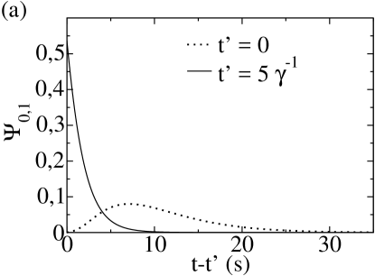
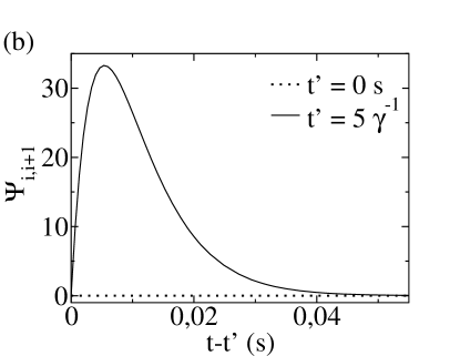
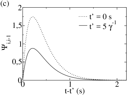
Figure 1: Waiting-time distributions. (a) $\Psi_{0,1}$ with $\alpha_{0}$=0.6 s^-1, $\beta_{0}$=1.07 s^-1, $\delta_{0}$=0.25 s^-1, $\epsilon_{0}$=0.225 s^-1, $Z_{0}$=0.25. (b) $\Psi_{i,i+1}$ with $\alpha$=160 s^-1, $\beta$=211 s^-1, $\delta$=4.5 s^-1, $\epsilon$=5.0 s^-1. (c) $\Psi_{i,i-1}$ with the same parameter values as (b). (a–c) $\gamma$=0.01 s^-1. The parameter values of (a–c) are the standard parameter set, which are used if not mentioned otherwise. The dwell time in state 0 decreases owing to the slow transient, but is always in the range of seconds (a). Upon entering state $i$, the dependences of $\Psi_{i,i+1}$ and $\Psi_{i,i-1}$ on $t-t^{\prime}$ with these large values of $\alpha$ and $\beta$ entail transitions either to $i+1$ very early or to $i-1$ later [see the abscissa range in (b) and (c)]. (d) Since $C_{i,i-1}$ is initially close to 1, the process lingers around state 0 until $t\approx\gamma^{-1}$, as shown by the simulation results for the average state index $\langle$i($\gamma$t)$\rangle$. When $C_{i,i-1}$ approaches $\frac{1}{2}$ at $t>\gamma^{-1}$, states further away from 0 with larger index $i$ are also reached.

The first-passage-time probability density $F_{0,N}(t)$ provides the probability of arrival for the first time in state $N$ in $(t,t+dt)$ when the process started in state $0$ at $t$=0. It is given by the probability flux out of the state range from 0 to $N-1$:

$$F_{0,N}(t) = -\frac{d}{dt}\sum_{k=0}^{N-1}P_{0,k}(t).$$ (27)

We denote its Laplace transform by $\tilde{F}_{0,N}(s)$. The moments of the first-passage-time distribution are given by van Kampen (2001)

$$\langle t^{n}\rangle=\left.(-1)^{n}\frac{\partial^{n}}{\partial s^{n}}\tilde{F}_{0,N}(s)\right|_{s=0}.$$ (28)

$F_{0,N}(t)$ can be determined by solving the master equations, setting state 0 as the initial condition and considering the state $N$ as absorbing, i.e., $\Psi_{N,N-1}\left(t,t-t^{\prime}\right)\equiv 0$:

$$0\stackrel{{\scriptstyle[}}{{\Psi}}_{i,i-1}]{\Psi_{0,1}}{\rightleftarrows}1\stackrel{{\scriptstyle[}}{{\Psi}}_{i,i-1}]{\Psi_{i,i+1}}{\rightleftarrows}2\ \ldots\ N-1\stackrel{{\scriptstyle[}}{{]}}{\Psi_{i,i+1}}{\rightarrow}N.$$ (29)

$F_{0,N}(t)$ captures not only the first-passage time $0\rightarrow N$, but also, to a good approximation, transitions starting at states with indices larger than 0 (and $<N$), since, owing to the initial bias, the process quickly moves into state 0 first and then slowly starts from there.

With the non-Markovian waiting-time distributions, the matrices $\tilde{G}(s)$ and $\tilde{H}(s)$ and the vector $\tilde{q}^{i}(s)$ of Eq. (17) specific to this problem are

$$\tilde{G}(s)_{1,2} =\tilde{g}_{0,1}(s),$$ (30)

$$\tilde{G}(s)_{2i,2i-1} =\tilde{G}(s)_{2i,2i+2}$$

$$=\tilde{g}_{i,i-1}(s),\quad i=1,\ldots,N-2,$$

$$\tilde{G}(s)_{2i+1,2i-1} =\tilde{G}(s)_{2i+1,2i+2}$$

$$=\tilde{g}_{i,i+1}(s),\quad i=1,\ldots,N-2,$$

$$\tilde{G}(s)_{2N-2,2N-3} =\tilde{g}_{N-1,N-2}(s),$$

$$\tilde{G}(s)_{2N-1,2N-3} =\tilde{g}_{N-1,N}(s),$$

$$\tilde{H}(s)_{1,2} =\tilde{h}_{0,1}(s),$$

$$\tilde{H}(s)_{2i,2i-1} =\tilde{H}(s)_{2i,2i+2}$$

$$=\tilde{h}_{i,i-1}(s),\quad i=1,\ldots,N-2,$$

$$\tilde{H}(s)_{2i+1,2i-1} =\tilde{H}(s)_{2i+1,2i+2}$$

$$=\tilde{h}_{i,i+1}(s),\quad i=1,\ldots,N-2,$$

$$\tilde{H}(s)_{2N-2,2N-3} =\tilde{h}_{N-1,N-2}(s),$$

$$\tilde{H}(s)_{2N-1,2N-3} =\tilde{h}_{N-1,N}(s),$$

$$\tilde{q}^{i}_{1}(s) =\Psi_{0,1}(s).$$

All other entries are equal to 0. Specifically for the first-passage problem, the matrices $D$ and $E$ are

$$E_{1,1} =-E_{i,i\pm 1}=-E_{1,2}=\lambda,\quad E_{i,i}=2\lambda,$$

$$D_{1,1} =D_{i,i}=-D_{i,i-1}=\lambda,\quad i=2,\ldots,N-1,$$

with all other entries being 0. The vector $\tilde{r}$ is equal to $\delta_{1i}$, $i=1,\ldots,N-1$. The Laplace transforms of the first-passage-time distributions are

$$\tilde{F}_{0,N}(s) = \tilde{I}_{N-1,N}^{0}(s)$$ (31)

with Eq. (8) and

$$\tilde{F}_{0,N}(s) = \lambda\big{[}\tilde{P}_{0,N-1}(s)-\tilde{P}_{0,N-1}(s+\gamma)\big{]}$$ (32)

with Eq. (2). Figure 2 (a) and (b) compare analytical results for the average first-passage time $T$ with the results of simulations. The agreement is very good, thus confirming the solutions given by Eqs. (17) and (20). This confirmation by simulations is important, since there is no method of solving difference equations that guarantees a complete solution.

Figure 2: The average first-passage time $T$ has a power-law dependence on the relaxation rate $\gamma$ of the initial transient of the form $\varpropto\gamma^{-\nu}$ for $\gamma\rightarrow 0$. (a, c) Results from solution of the generalized master equation (17) and Eqs. (23)–(25). (b, d) Results from solution of the asymptotically Markovian master equation (20) and Eq. (22) with $\lambda=0.4$ s^-1. $N_{\nu}$ is the number of edges with identical waiting-time distributions. $N_{\nu}$ is equal to $N-1$ in (c) and to $N$ in (d). The variable $u$ in (c) and (d) is defined as $u=N_{\nu}/(N_{\nu}+1)$. In (a) and (b), simulations (lines) are compared with analytical results ($\circ$).

IV Scaling of the average first-passage time with the relaxation rate

Figure 2 shows results for the average first-passage time $T$ across four orders of magnitude of the relaxation rate $\gamma$. The results strongly suggest that $T$ grows according to a power law $\gamma^{-\nu}$ with decreasing $\gamma$, if $\gamma$ is sufficiently small. The exponent exhibits a simple dependence on the number $N_{\nu}$ of edges with identical waiting-time distributions. That number is equal to $N$ for processes according to Eqs. (22) and to $N-1$ for processes obeying Eqs. (23)– (25), since the $0\rightarrow 1$ transition is different there. The exponent $\nu$ depends to leading order on $N_{\nu}$ like $N_{\nu}/(N_{\nu}+1)$. This applies to both the asymptotically Markovian and non-Markovian waiting-time distributions, and to both parameter sets of waiting-time distributions simulated in the non-Markovian case.

The exponent $\nu$ is equal to $\frac{1}{2}$ for $N_{\nu}=1$, as has previously been shown analytically for $f_{i,i\pm 1}$ according to Eq. (22) (see Dupont et al. (2016), Chapter 5). The process is very unlikely to reach large $N$ with a bias toward 0, even if this is only small. Hence, the random walk “waits” until the transient is over and symmetry of the transition rates has been reached [see Fig. 1(d)], and then goes to $N$. This waiting contributes a time $\varpropto\gamma^{-1}$ to $T$, and $\nu$ approaches 1 for large $N_{\nu}$.

The average first-passage time for a symmetric random walk increases with $N$ like $N(N-1)$ Jouini and Dallery (2008), i.e., it is very long for large $N$. We see a contribution of the transient to $T$ only if relaxation is slow enough for $\gamma^{-1}$ to be comparable to this long time. Consequently, $T$ is essentially independent of $\gamma$ for large $\gamma$ and large $N$ (see $N=200$ in Fig. 2(a, b)).

V Resonant length

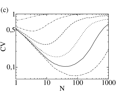
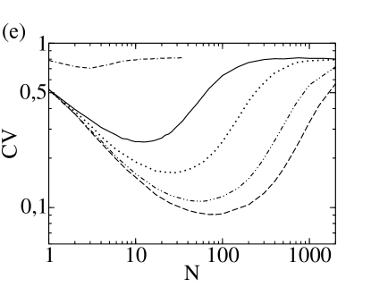
Figure 3: The coefficient of variation CV shows a pronounced minimum in its dependence on the chain length $N$. (a) Analytical results using the solution of the generalized master equation (17) and Eqs. (23)–(25) with $\alpha=0.4$ s^-1 and $\beta=0.5275$ s^-1. (b) Analytical results using the solution of the asymptotically Markovian master equation (20) and Eq. (22) with $\lambda=0.4$ s^-1. (c, d) Simulations using Eqs. (23)–(25). In (c), from top to bottom, $\gamma=1$, $1.156\times 10^{-1}$, $1.156\times 10^{-2}$, $1.015\times 10^{-3}$, $1.156\times 10^{-4}$, and $10^{-5}$ s^-1; $C_{i,i-1}(t^{\prime}=\infty)\gtrsim\frac{1}{2}$. In (d), $\alpha=0.4$ s^-1, $\beta=0.5275$ s^-1, and, from top to bottom $\gamma=0.1$, $1.156\times 10^{-2}$, $1.015\times 10^{-3}$, $1.156\times 10^{-4}$, and $10^{-5}$ s^-1; $C_{i,i-1}(t^{\prime}=\infty)\lesssim\frac{1}{2}$. (e) Simulations using Eqs. (22) with $\lambda=0.4$ s^-1, $C_{i,i-1}(t^{\prime}=\infty)=\frac{1}{2}$, $\gamma=1$, $10^{-3}$, $10^{-4}$, $10^{-5}$, and $10^{-5.5}$ s^-1. (f) Properties of the minima of the CV as a function of the relaxation rate $\gamma$. The splitting probability $C_{i,i-1}(t^{\prime}=T)$ at the minimum changes only slightly over four orders of magnitude of $\gamma$ [between 0.515 and 0.565 in (c), 0.531 and 0.564 in (d), and 0.516 and 0.555 in (e)]. The dependence of the minimal CV on $\gamma$ shown in (d) is well fitted by $\gamma^{0.181}$ in the asymptotically Markovian case (c), and by $\gamma^{0.186}$ for $\gamma<2\times 10^{-3}$ s^-1 for the parameter values in (b), but deviates from a power law for the values in (a).

The coefficient of variation CV [= standard deviation (SD)/average $T$] of the first-passage time reflects the relative fluctuations. Its dependence on the chain length $N$ is illustrated in Fig. 3. CV increases monotonically with increasing $\gamma$. Its dependence on $N$ is not monotonic. We find a pronounced minimum of CV($N$) for small values of $\gamma$, where the minimal value is up to one order of magnitude smaller than CVs with $N=1$ and with large $N$. Both simulations and analytical results show this behavior.

How can we get a heuristic understanding of the decrease in CV with decreasing $\gamma$ and initially with increasing $N$? The lingering close to state 0 shown in Fig. 1(d) means that states with index $i$ larger than 1 are not reached before a time $t\approx\gamma^{-1}$ with almost certainty. This initial part of the process contributes to $T$ but little to SD. Hence, its growth with decreasing $\gamma$ and (initially) increasing $N$ decreases CV. Additionally, the standard deviation is determined by the rates and splitting probabilities at the end of the transient, which are more favorable for reaching $N$ than the splitting probabilities at the beginning. It is therefore less affected than the average by the $\gamma$ values. This also causes a decrease in CV with decreasing $\gamma$.

To gain more insight into the $N$ dependence of CV, we look at processes with constant transition rates and a symmetric process with transient rates but constant splitting probabilities $C_{i,i-1}=C_{i,i+1}=\frac{1}{2}$ [see Eq. (33)]. The permanently symmetric process exhibits only a very shallow minimum, and the minimal value of CV appears to be independent of $\gamma$ [Fig. 4(a): discrete case]. Processes with constant transition rates exhibit decreasing CV with decreasing $C_{i,i-1}$ Jouini and Dallery (2008) [Fig. 4(b)]. However, this decrease is minor and does not explain the data in Fig. 3 in the range $C_{i,i-1}\geq\frac{1}{2}$ covered by the transient.

The comparison shows that the dynamics of the splitting probabilities provide the major part of the reduction in CV with increasing $N$ in Fig. 3. The splitting probability $C_{i,i-1}$ relaxes from 1 to its asymptotic value set by the parameters of the process. The larger the value of $N$, the later is the absorbing state reached and the smaller is the value of $C_{i,i-1}$ when it is reached. As long as $C_{i,i-1}(t^{\prime}=T)$ decreases sufficiently rapidly with increasing $N$, so does CV. At values of $N$ such that $\gamma T\gtrsim 2$, the decrease in $C_{i,i-1}(t^{\prime}=T)$ is negligible, and CV starts to rise again with increasing $N$ toward its large-$N$ value.

These considerations suggests that the $N$ with minimal CV could be fixed by a specific value of the splitting probability. This value of $C_{i,i-1}$ cannot be smaller than $\frac{1}{2}$, since we would expect a monotonically decreasing CV in that regime [the $N^{-\frac{1}{2}}$ regime in Fig. 3(d)]. Since this should hold also for minima with $N\gg 1$, this value of $C_{i,i-1}$ also cannot be much larger than $\frac{1}{2}$, since $T$ would then diverge. This is confirmed by the results shown in Fig. 3(f). The splitting probability $C_{i,i-1}(t^{\prime}=T)$ at the minimum changes by less than 8% over four orders of magnitude of $\gamma$, and is slightly larger than $\frac{1}{2}$. Hence, CV starts to rise again when the length $N$ is so large that the average first-passage time is long enough for $C_{i,i-1}(t^{\prime}=T)$ to approach the symmetric limit .

The value of CV($N=\infty$) depends on $\gamma$ in the case with non-Markovian waiting-time distributions. It is 1 for large $\gamma$ values, since the asymptotic splitting probability $C_{i,i-1}(t^{\prime}=\infty)$ is larger than $\frac{1}{2}$ [Fig. 3(c); see also Fig. 4(b)]. CV($N=\infty$) is approximately equal to $\sqrt{2/3}$ for small values of $\gamma$, since $C_{i,i-1}(t^{\prime}=\infty)\approx\frac{1}{2}$ applies in that case [Fig. 3(c)]. CV($N=\infty$) is exactly $\sqrt{2/3}$ with asymptotically Markovian waiting-time distributions [Fig. 3(e)].

The parameter values in Fig. 3(d) entail $C_{i,i-1}(t^{\prime}=\infty)\lesssim\frac{1}{2}$. The process has a bias toward $N$ and we see the well-known behavior CV($N$) $\propto N^{-\frac{1}{2}}$ for large $N$. The onset of the $N^{-\frac{1}{2}}$ behavior moves to smaller $N$ with increasing values of $\gamma$ until finally the minimum of the CV is lost. We found minima if $\gamma^{-1}\gtrsim$ (four times the average state dwell time), but we have not determined a precise critical value.

The transition from the CV of $\Psi_{0,1}$ to CV($N=\infty$) for large values of $\gamma$ is monotonic in Fig. 3(c) for the asymptotically non-Markovian case. The asymptotically Markovian system exhibits a minimum even for large $\gamma$ values [$\gamma\approx\lambda$: Fig. 3(e)]. However, it is comparably shallow, and is in line with the results of Jouini and Dallery for systems without transient Jouini and Dallery (2008) [Fig. 4(b)].

Figure 4: (a) The coefficient of variation CV shows a shallow minimum in its dependence on the chain length $N$ with processes that are discrete and always symmetric (symbols), but not for the continuous symmetric case (lines), which is the solution of the Fokker–Planck equation (34). The symbols + and $\circ$ show results from simulations using Eq. (33). The calculations used $\lambda=0.4$ s^-1 (all), and $\gamma=10^{-4}$ s^-1 ($\circ$, full line), $\gamma=3.6\times 10^{-6}$ s^-1 (+, dashed line). The value of the CV at the minimum is essentially unaffected by the change in the value of $\gamma$. The $\bigtriangleup$ marks the analytical result with $N=1$ for both discrete cases, which are indistinguishable at the resolution of the plot and are in agreement with the simulations. The continuous large-$L$ and discrete large-$N$ results agree very well. (b) CV with constant transition rates calculated using the equations of Jouini and Dallery Jouini and Dallery (2008). CV $\geq\sqrt{2/3}$ holds for $C_{i,i-1}\geq\frac{1}{2}$.

VI Discussion and Conclusion

VI.1 (Generalized) master equation with exponential time dependence of rates and waiting-time distributions

In general, stochastic processes occur in changing environments or may be subjected to control. The corresponding mathematical description is provided by (generalized) master equations with time-dependent coefficients. The analytical solution of these equations is complicated even in the simplest case [see Eq. (A)] Skupin, A. and Falcke, M. (2010). The Laplace-transform approach is not applicable in general, but the exponential time dependences of the master equation (2) or the generalized master equation (8) with (9) do allow the transform to be performed on them, leading to difference equations in Laplace space. The solutions of these equations are given by Eqs. (17) and (20), resp. To the best of our knowledge, this is a novel (and efficient) method of solving the generalized master equation with this type of time dependence in the kernel, or the master equation with this type of time-dependent rates.

Equations (17) and (20) also apply in the case of state schemes more complicated than that in (21). It is only necessary to make appropriate changes to the definitions of $\tilde{H}(s)$ and $\tilde{G}(s)$ or of $D$ and $E$. Hence, we can use the method presented here to investigate the dynamics of complicated networks in a transient. This is of interest for studies of ion-channel dynamics Sneyd et al. (2004); Gin et al. (2009), transport in more than one spatial dimension, gene regulatory networks, and many other applications. Many quantities of interest in these investigations are moments of first-passage type and thus can be calculated from the derivatives of the Laplace transforms. Some of these calculations might require knowledge of the probability time dependence $P_{i,j}(t)$, i.e., the residues of $\tilde{P}_{i,j}(s)$. In many cases, determination of these residues will be only slightly more complicated than for the system without transient, since all terms arising from the transient involve the same factors, but with shifted argument, together with the matrix $\tilde{H}(s)$. In general, if we know the set of residues $\{S_{0}\}$ of the Laplace transform of the system without transient and the matrix $\tilde{H}(s)$, we can immediately write down the residues of the Laplace transform of the system with transient by shifting $\{S_{0}\}$ by integer multiples of $\gamma$. This allows easy generalization of many results and might be of particular interest for renewal theory Cox (1970); van Kampen (2001).

VI.2 The average first-passage time

The average first-passage time decreases with increasing relaxation rate according to a power law, if the transient is sufficiently slower than the time scale of the individual steps (Fig. 2). The exponent depends on the chain length to leading order like $-N/(N+1)$. Remarkably, this behavior has been found for substantially different parameters in both the asymptotically non-Markovian and asymptotically Markovian cases, and therefore appears to be rather universal.

VI.3 Resonant length

Transients can substantially reduce the coefficient of variation. We have found a monotonic decrease of CV with decreasing $\gamma$ when the relaxation rate is slow compared with state transition rates. CV exhibits a minimum in its dependence on the chain length $N$ (Fig. 3) if the transient is slow compared with state dynamics. This minimum exists for both asymptotically Markovian and non-Markovian discrete systems. At a time-scale separation between the state transition rates and the transient of about $10^{6}$, the CV at the minimum is reduced by about one order of magnitude compared with CV($N=1$).

Exploiting our results for control purposes, we can use a transient if more precise arrival timing at the outcome of a process is desired. Applying a transient that relaxes a bias toward 0 reduces CV. In the context of charge carrier transport, such a transient could be realized by a time-dependent electric field. If we include the rising part of CV($N$) beyond the minimum in our consideration and consider all CVs smaller than CV($N=1$) as reduced, we may still see a reduction of CV even if the average first-passage time is an order of magnitude longer than $\gamma^{-1}$. Hence, the initial transient may have surprisingly long-term consequences and is therefore a rather robust method for CV reduction. Additionally, or if a transient is given, the state and step number can be used for optimizing the precision of arrival time. The optimum may also be at smaller lengths than that of the non-optimized process; i.e., optimization of precision may even lead to acceleration.

VI.4 How can negative feedback robustly reduce noise in timing?

Most studies investigating the effect of negative feedback have focused on amplitude noise—we are looking at noise in timing. Timing noise substantially reduces information transmission in communication systems. Variability in timing and protein copy numbers in gene expression or cell differentiation causes cell variability Yurkovsky and Nachman (2013); Hormoz et al. (2016). Therefore, many studies have investigated the role of noise in gene regulatory networks and have found that immediate negative feedback is not suitable for reducing timing noise Kontogeorgaki et al. (2016); Hinczewski and Thirumalai (2016); Ghusinga et al. (2017). This agrees with our results for large $\gamma$ values.

We have shown that slow recovery from negative feedback is a robust means of noise reduction. The recovery process corresponds to the slow transient in our present study. Negative feedback terminating the excited state is a constitutive element of many systems generating sequences of pulses or spikes, such as oscillating chemical reactions Totz et al. (2015); Falcke and Engel (1994), the electrical membrane potential of neurons Kandel et al. (1991), the sinoatrial node controlling the heart beat Pohl et al. (2016), the tumor suppressor protein p53 Vousden and Lane (2007); Mönke et al. (2017), Ca²⁺ spiking in eukaryotic cells Falcke (2004); Skupin et al. (2008); Thurley et al. (2014), cAMP concentration spikes in Dictyostelium discoideum cells and other cellular signaling systems Goldbeter (1996); Falcke and Levine (1998).

In particular, our results apply to noisy excitable spike generators in cells, where single molecular events or sequences of synaptic inputs form a discrete chain of states toward the threshold. Beside examples from membrane potential spike generation Grewe et al. (2017), Ca²⁺ spiking and p53 pulse sequences have been shown to be noise-driven excitable systems Mönke et al. (2017); Thurley et al. (2014); Skupin et al. (2008); Thurley and Falcke (2011). The information content of frequency-encoding spiking increases strongly with decreasing CV of spike timing Skupin and Falcke (2009). A value of the coefficient of variation between 0.2 and 1.0 has been measured for the sequence of interspike intervals of intracellular Ca²⁺ signaling Skupin et al. (2008); Thurley et al. (2014); Dragoni et al. (2011); Cao et al. (2014); Lembong et al. (2017). Hence, CV is decreased compared with that of a Poisson process and even compared with that for first passage of a symmetric random walk. The experimental data are also compatible with the finding that the slower the recovery from negative feedback, the lower is CV Skupin et al. (2008); Thurley et al. (2014); Dragoni et al. (2011); Cao et al. (2014); Lembong et al. (2017). This strongly suggests that this ubiquitous cellular signaling system uses the mechanism of noise reduction described here to increase information transmission.

Optimal noise amplitudes minimize the CV of interspike intervals in noisy excitable systems Jung and Mayer-Kress (1995); Pikovski and Kurths (1997); Gang et al. (1993); Beato et al. (2008); Lindner et al. (2004), which has been termed coherence resonance. Our results define the conditions of optimal CV reduction in terms of system properties—an optimal number of steps from the inhibited state to the excitation threshold during slow recovery. At the same time, our results shed light on new aspects of coherence resonance, and indeed may indicate that a more fundamental phenomenon underlies it. Since we believe excitable systems to be one of the most important applications of our results, we have chosen the term resonant length.

Coming back to the widely used graphic example, what can the drunkard learn from our results? If he chooses a pub at the right distance from home, he will arrive home sober and relatively in time for breakfast.

Appendix A The symmetric asymptotically Markovian case and its continuum limit

The permanently symmetric case with a transient is defined by

$$f_{i,i\pm 1}(t) = \lambda\left(1-e^{-\gamma t}\right).$$ (33)

Its continuum limit on a domain of length $L$ (with spatial coordinate $x$) satisfies

$$\frac{\partial P(x,t)}{\partial t} = 2\lambda\left(1-e^{-\gamma t}\right)\frac{\partial^{2}P(x,t)}{\partial x^{2}}.$$ (34)

The Fokker–Planck equation (34) can be solved after applying a time transformation $t\rightarrow\tau$:

$$\tau(t)=2\int_{0}^{t}f_{i,i\pm 1}(t^{\prime})\,dt^{\prime}=2\lambda\left(t+\frac{e^{-\gamma t}}{\gamma}-\frac{1}{\gamma}\right).$$ (35)

The boundary and initial conditions, $P(L,t)=0$, $\partial P(x,t)/\partial x|_{x=0}=0$, and $P(x,0)=\delta(x)$ specify the first-passage problem. We find

$$P(x,\tau)=\frac{2}{L}\sum_{n=0}^{\infty}\cos\left(k_{n}x\right)e^{-k_{n}^{2}\tau},$$ (36)

where $k_{n}=\pi(2n+1)/(2L)$. The $i$th moment of the first-passage time is given by

$$\langle t^{i}\rangle = \int_{0}^{\infty}t^{i}F(t)\,dt,$$ (37)

$$F(t) = -\frac{d}{dt}\int_{0}^{L}P(x,\tau(t))\,dx.$$ (38)

With $a_{n}=2\lambda k_{n}^{2}/\gamma$, we obtain

$$\langle t\rangle=\frac{4}{\pi\gamma}\sum_{n=0}^{\infty}\frac{(-1)^{n}}{2n+1}e^{a_{n}}a_{n}^{-a_{n}}\Gamma\left(a_{n},a_{n}\right),$$ (39)

where $\Gamma(y,x)$ is the lower incomplete gamma function. The second moment is

$$\langle t^{2}\rangle={} \frac{32L^{4}}{\lambda^{2}\pi^{5}}\sum_{n=0}^{\infty}\frac{(-1)^{n}}{(2n+1)^{5}}e^{a_{n}}$$

$$\times{}_{2}F_{2}\left(\left\{a_{n},a_{n}\right\};\left\{a_{n}+1,a_{n}+1\right\};-a_{n}\right)$$ (40)

where ${}_{2}F_{2}$ is a hypergeometric function. Results for CV are shown in Fig. 4(a). In the continuous case, CV does not exhibit a minimum in its dependence on the length $L$. Interestingly, CV at small $L$ is very close to the minimum value of the discrete case.

The $a_{n}$ are small for $L\gg\lambda/\gamma$. Therefore, in that limit, we can approximate the incomplete $\Gamma$ function and hypergeometric function by

$$\Gamma\left(a_{n},a_{n}\right)\approx a_{n}^{a_{n}-1}\ e^{-a_{n}},$$

$$e^{a_{n}}\,{}_{2}F_{2}\left(\left\{a_{n},a_{n}\right\};\left\{a_{n}+1,a_{n}+1\right\};-a_{n}\right)\approx 1,$$

and find

$$\mathrm{CV}(L\gg\lambda/\gamma)\approx\sqrt{\frac{5}{3}\frac{L^{4}}{\lambda^{2}}\frac{\lambda^{2}}{L^{4}}-1}=\sqrt{\frac{2}{3}}\;,$$ (41)

i.e., CV approaches monotonically the value of a symmetric random walk with constant transition rates for large $L$.

Appendix B Numerical methods

Evaluation of Eqs. (17) and (20): If $N$ is large and the ratio between the fastest state transition rate and the relaxation rate $\gamma$ is larger than $10^{4}$, high precision of the numerical calculations is required for the use of Eqs. (17) and (20). A priori known values like $\tilde{I}_{N-1,N}^{0}(s=0)=1$ can be used to monitor the precision of the calculations. The matrix products become very large at intermediate values of $j\gamma$ during the summation in Eqs. (17) and (20), and their sign alternates such that two consecutive summands nearly cancel. Intermediate summands are of order larger than $10^{17}$, and thus we face loss of significant figures even with the numerical floating-point number format long double. We used Arb, a C numerical library for arbitrary-precision interval arithmetic Johansson (2017), to circumvent this problem. It allows for arbitrary precision in calculations with Eqs. (17) and (20). Computational speed is the only limitation with this library and has determined the parameter range for which we established analytical results. We were able to go to a time-scale separation of $\approx 10^{6}$ using this library.

Simulation method: We use simulations for comparison with the analytic solutions and for systems with large $N$. The $\Psi_{l,j}(t,t-t^{\prime})$ are functions only of $t$ for a given $t^{\prime}$. Since $t^{\prime}$ is the time when the process moved into state $l$, it is always known. The simulation algorithm generates in each iteration the cumulative distribution $\int_{t^{\prime}}^{t}d\theta\,\sum_{i=1}^{N_{\mathrm{out}}^{(l)}}\Psi_{l,j_{i}}(\theta,\theta-t^{\prime})$ and then draws the time $t_{\mathrm{tr}}$ for the next transition. The specific transition is chosen from the relative values $\Psi_{l,j_{k}}(t_{\mathrm{tr}},t_{\mathrm{tr}}-t^{\prime})/\sum_{i=1}^{N_{\mathrm{out}}^{(l)}}\Psi_{l,j_{i}}(t_{\mathrm{tr}},t_{\mathrm{tr}}-t^{\prime})$ by a second draw. We verified the simulation algorithm by comparison of simulated and calculated stationary probabilities [Eq. (45)], splitting probabilities at a variety of $t^{\prime}$ values, simulations without recovery (“$\gamma=\infty$”) and the comparisons in Fig. 2. We used at least 20 000 sample trajectories to calculate moments and up to 160 000 to determine the location of the minima of CV.

Appendix C The stationary probabilities

The stationary probabilities are reached for $t\rightarrow\infty$. This entails $\Psi_{i,i\pm 1}(t,t-t^{\prime})=\Psi_{i,i\pm 1}^{\infty}(t-t^{\prime})=g_{i,i\pm 1}\left(t-t^{\prime}\right)$. We start from the idea that the stationary probability $P_{i}$ of being in state $i$ is equal to the ratio of the total average time $T_{i}$ spent in $i$ divided by the total average time for large $t$:

$$P_{i} = \frac{T_{i}}{\sum_{j}^{N}T_{j}}.$$ (42)

$T_{i}$ is equal to the number $N_{i}$ of visits to state $i$ multiplied by the average dwell time $t_{i}$ in $i$:

$$P_{i} = \frac{t_{i}N_{i}}{\sum_{j}^{N}t_{j}N_{j}}.$$ (43)

Each visit to state $i$ starts with a transition to $i$. The average number of transitions into $i$ is equal to the number of visits to its neighboring states multiplied by the probability that the transition out of the neighboring states is toward $i$. With the splitting probabilities $C_{i,i\pm 1}(t=\infty)$ denoted by $C_{i,i\pm 1}$, the $N_{i}$ obey

$$N_{i} = C_{i-1,i}N_{i-1}+C_{i+1,i}N_{i+1}.$$ (44)

Dividing by the total number of visits $\sum_{j=0}^{N}N_{j}$, we get

$$n_{i} = C_{i-1,i}n_{i-1}+C_{i+1,i}n_{i+1},$$ (45)

$$1 = \sum_{j=0}^{N}n_{j},$$ (46)

$$P_{i} = \frac{t_{i}n_{i}}{\sum_{j=0}^{N}t_{j}n_{j}}.$$ (47)

We write Eq. (45) in matrix form, $\mathbb{M}\mathbb{n}=\mathbb{0}$, with

$$M_{i,i\pm 1} = -\tilde{g}_{i\pm 1,i}(0),$$ (48)

$$M_{i,i} = 1,$$ (49)

and all other entries 0. We checked for $N=2,3,4$ that $\det\mathbb{M}=0$ holds. Equation (45) determines $\mathbb{n}$ only up to a common factor, which is then fixed by Eq. (46).

The average dwell times $t_{i}$ in the states are initially affected by the recovery from negative feedback, but are constant at large $t$. They have contributions $t_{i,i\pm 1}$ from both transitions to $i\pm 1$, with weights set by $C_{i,i\pm 1}$:

$$t_{i} = C_{i,i+1}t_{i,i+1}+C_{i,i-1}t_{i,i-1}.$$ (50)

$C_{i,i\pm 1}t_{i,i\pm 1}=-(\partial/\partial s)\tilde{g}_{i,i\pm 1}|_{s=0}$ holds owing to the normalization of the $\Psi_{i,i\pm 1}$. This leads finally to

$$t_{i} = \left.-\frac{\partial}{\partial s}\left(\tilde{g}_{i,i-1}+\tilde{g}_{i,i+1}\right)\right|_{s=0}.$$ (51)

To give a specific example, the stationary-state probabilities for $N=2$ are

$$\mathbb{P}={} \frac{1}{(\partial/\partial s)\left(C_{1,0}\tilde{g}_{0,1}+\tilde{g}_{1,0}+\tilde{g}_{1,2}+C_{1,2}\tilde{g}_{2,1}\right)}$$

$$\left.\times\begin{pmatrix}C_{1,0}(\partial/\partial s)\tilde{g}_{0,1}\\[4.0pt] (\partial/\partial s)\left(\tilde{g}_{1,0}+\tilde{g}_{1,2}\right)\\[4.0pt] C_{1,2}(\partial/\partial s)\tilde{g}_{2,1}\end{pmatrix}\right|_{s=0}.$$

References

- Wei et al. (2000) Q.-H. Wei, C. Bechinger, and P. Leiderer, Science 287, 625 (2000).
- Chupeau et al. (2015) M. Chupeau, O. Bénichou, and R. Voituriez, Nature Physics 11, 844 (2015).
- Guérin et al. (2016) T. Guérin, N. Levernier, O. Bénichou, and R. Voituriez, Nature 534, 356 (2016).
- Molini et al. (2011) A. Molini, P. Talkner, G. Katul, and A. Porporato, Physica A: Statistical Mechanics and its Applications 390, 1841 (2011).
- Panja (2010) D. Panja, Journal of Statistical Mechanics: Theory and Experiment 2010, P06011 (2010).
- Turiv et al. (2013) T. Turiv, I. Lazo, A. Brodin, B. I. Lev, V. Reiffenrath, V. G. Nazarenko, and O. D. Lavrentovich, Science 342, 1351 (2013).
- Démery et al. (2014) V. Démery, O. Bénichou, and H. Jacquin, New Journal of Physics 16, 053032 (2014).
- Ernst et al. (2012) D. Ernst, M. Hellmann, J. Kohler, and M. Weiss, Soft Matter 8, 4886 (2012).
- Baranovskii (2014) S. D. Baranovskii, Physica Status Solidi (b) 251, 487 (2014).
- Metzler and Klafter (2000) R. Metzler and J. Klafter, Physics Reports 339, 1 (2000).
- Blumen et al. (2002) A. Blumen, J. Klafter, and I. Sokolov, Phys. Today 55, 48 (2002).
- Hofmann and Ivanyuk (2003) H. Hofmann and F. A. Ivanyuk, Phys Rev Lett 90, 132701 (2003).
- Sokolov and Klafter (2005) I. M. Sokolov and J. Klafter, Chaos: An Interdisciplinary Journal of Nonlinear Science 15, 026103 (2005).
- Shlesinger (2006) M. F. Shlesinger, Nature 443, 281 (2006).
- van Kampen (2001) N. van Kampen, Stochastic processes in physics and chemistry (North-Holland, Amsterdam, 2001).
- Oppenheim et al. (1977) I. Oppenheim, K. E. Shuler, and G. H. Weiss, Stochastic processes in chemical physics: the master equation (MIT Press, 1977).
- Bénichou et al. (2010) O. Bénichou, C. Chevalier, J. Klafter, B. Meyer, and R. Voituriez, Nature Chemistry 2, 472 (2010).
- Berg (1993) H. C. Berg, Random walks in Biology (Princeton University Press, 1993).
- Gazzola et al. (2009) M. Gazzola, C. J. Burckhardt, B. Bayati, M. Engelke, U. F. Greber, and P. Koumoutsakos, PLOS Computational Biology 5, 1 (2009).
- Bressloff and Newby (2013) P. C. Bressloff and J. M. Newby, Rev Mod Phys 85, 135 (2013).
- Ivanov et al. (2016) I. V. Ivanov, X. Qian, and R. Pal, Emerging Research in the Analysis and Modeling of Gene Regulatory Networks (IGI Global, Hershey, PA, 2016).
- Scott (1997) L. O. Scott, Mathematical Finance 7, 413 (1997).
- Steele (2000) J. M. Steele, Stochastic Calculus and Financial Applications, edited by B. Rozovskii and M. Yor, Stochastic Modelling and Applied Probabilty, Vol. 45 (Springer, 2000).
- Mayo et al. (2011) M. L. Mayo, E. J. Perkins, and P. Ghosh, BMC Bioinformatics 12, S18 (2011).
- Winter and von Hippel (1981) R. B. Winter and P. H. von Hippel, Biochem 20 (1981).
- Berg et al. (1981) O. G. Berg, R. B. Winter, and P. H. von Hippel, Biochem 20 (1981).
- Riggs et al. (1970a) A. D. Riggs, S. Suzuki, and S. Bourgeois, J. Mol. Biol 48 (1970a).
- Riggs et al. (1970b) A. D. Riggs, S. Bourgeois, and M. Cohn, J. Mol. Biol 53 (1970b).
- Shimamoto (1999) N. Shimamoto, J. Biol. Chem 274 (1999).
- Albert et al. (2012) M. Albert, G. Haack, C. Flindt, and M. Büttiker, Phys Rev Lett 108, 186806 (2012).
- Scher and Lax (1973) H. Scher and M. Lax, Phys. Rev. B 7, 4491 (1973).
- Britton (2010) T. Britton, Mathematical Biosciences 225, 24 (2010).
- Redner et al. (2014) S. Redner, R. Metzler, and G. Oshanin, eds., First-Passage Phenomena and Their Applications (World Scientific Publishing Co. Pte. Ltd., 2014).
- Redner (2001) S. Redner, A Guide to First-Passage Processes (Cambridge University Press, 2001).
- Condamin et al. (2007) S. Condamin, O. Bénichou, V. Tejedor, R. Voituriez, and J. Klafter, Nature 450, 77 (2007).
- Shlesinger (2007) M. F. Shlesinger, Nature 450, 40 (2007).
- Hormoz et al. (2016) S. Hormoz, Z. S. Singer, J. M. Linton, Y. E. Antebi, B. I. Shraiman, and M. B. Elowitz, Cell Systems 3, 419 (2016).
- García-Ojalvo and Schimansky-Geier (2000) J. García-Ojalvo and L. Schimansky-Geier, J.Stat.Phys. 101, 473 (2000).
- Kostur et al. (2003) M. Kostur, X. Sailer, and L. Schimansky-Geier, Fluctuation and Noise Letters 03, L155 (2003).
- Lindner et al. (2004) B. Lindner, J. Garcia-Ojalvo, A. Neimann, and L. Schimansky-Geier, Physics Reports 392, 321 (2004).
- Falcke et al. (1992) M. Falcke, M. Bär, H. Engel, and M. Eiswirth, The Journal of Chemical Physics 97, 4555 (1992).
- Keener and Sneyd (1998) J. Keener and J. Sneyd, Mathematical Physiology (Springer, New York, 1998).
- Scott (1975) A. C. Scott, Rev Mod Phys 47, 487 (1975).
- Pei et al. (1995) X. Pei, K. Bachmann, and F. Moss, Physics Letters A 206, 61 (1995).
- Cross and Hohenberg (1993) M. Cross and P. Hohenberg, Rev Mod Phys 65, 851 (1993).
- Mikhailov (1994) A. Mikhailov, Foundations of Synergetics, Springer Series in Synergetics, Vol. 1,2 (Springer, 1994).
- Ebeling and Feistel (1986) W. Ebeling and R. Feistel, Physik der Selbstorganisation und Evolution (Akademieverlag Berlin, 1986).
- Franosch et al. (2011) T. Franosch, M. Grimm, M. Belushkin, F. M. Mor, G. Foffi, and L. Forro, Nature 478, 85 (2011).
- Esposito and Lindenberg (2008) M. Esposito and K. Lindenberg, Phys Rev E 77, 051119 (2008).
- Albert et al. (2016) M. Albert, D. Chevallier, and P. Devillard, Physica E 76, 209 (2016).
- Koch et al. (2005) J. Koch, M. E. Raikh, and F. von Oppen, Phys Rev Lett 95, 056801 (2005).
- Hille (2001) B. Hille, Ion Channels of excitable Membranes, 3rd ed. (Sinauer Assoicates, Inc. Publishers, Sunderland, MA USA, 2001).
- Sneyd et al. (2004) J. Sneyd, M. Falcke, J. F. Dufour, and C. Fox, Progress in Biophysics and Molecular Biology 85, 121 (2004), modelling Cellular and Tissue Function.
- Kenkre (1978) V. Kenkre, Physics Letters A 65, 391 (1978).
- Hänggi and Talkner (1985) P. Hänggi and P. Talkner, Phys Rev A 32, 1934 (1985).
- Masoliver et al. (1986) J. Masoliver, K. Lindenberg, and B. J. West, Phys Rev A 34, 2351 (1986).
- Metzler et al. (1999) R. Metzler, E. Barkai, and J. Klafter, EPL (Europhysics Letters) 46, 431 (1999).
- Davies et al. (1992) J. H. Davies, P. Hyldgaard, S. Hershfield, and J. W. Wilkins, Phys. Rev. B 46, 9620 (1992).
- Kenkre et al. (1973) V. M. Kenkre, E. W. Montroll, and M. F. Shlesinger, J Stat Phys 9, 45 (1973).
- Montroll and Scher (1973) E. W. Montroll and H. Scher, J Stat Phys 9, 101 (1973).
- Burshtein et al. (1986) A. I. Burshtein, A. A. Zharikov, and S. I. Temkin, Theoretical and Mathematical Physics 66, 166 (1986).
- Chechkin et al. (2005) A. V. Chechkin, R. Gorenflo, and I. M. Sokolov, Journal of Physics A: Mathematical and General 38, L679 (2005).
- Sokolov and Klafter (2007) I. Sokolov and J. Klafter, Chaos, Solitons & Fractals 34, 81 (2007).
- Dupont et al. (2016) G. Dupont, M. Falcke, V. Kirk, and J. Sneyd, Models of Calcium Signalling, edited by S. Antman, L. Greengard, and P. Holmes, Interdisciplinary Applied Mathematics, Vol. 43 (Springer, 2016).
- Jouini and Dallery (2008) O. Jouini and Y. Dallery, Mathematical Methods of Operations Research 68, 49 (2008).
- Note (1) The minima of the CV are less correlated with a specific value of the product , since at the minima changes by about 20% in Fig. 3(c) and about 80% in Fig. 3(d) and (e) across the -range.
- Skupin, A. and Falcke, M. (2010) Skupin, A. and Falcke, M., Eur. Phys. J. Special Topics 187, 231 (2010).
- Gin et al. (2009) E. Gin, M. Falcke, L. E. Wagner, D. I. Yule, and J. Sneyd, Biophys.J. 96, 4053 (2009).
- Cox (1970) D. Cox, Renewal Theory (Methuen & Co, 1970).
- Yurkovsky and Nachman (2013) E. Yurkovsky and I. Nachman, Briefings in Functional Genomics 12, 90 (2013).
- Kontogeorgaki et al. (2016) S. Kontogeorgaki, R. J. Sánchez-García, R. M. Ewing, K. C. Zygalakis, and B. D. MacArthur, Scientific Reports 7, 532 (2016).
- Hinczewski and Thirumalai (2016) M. Hinczewski and D. Thirumalai, The Journal of Physical Chemistry B 120, 6166 (2016).
- Ghusinga et al. (2017) K. R. Ghusinga, J. J. Dennehy, and A. Singh, Proc Nat Acad Sci USA 114, 693 (2017).
- Totz et al. (2015) J. F. Totz, R. Snari, D. Yengi, M. R. Tinsley, H. Engel, and K. Showalter, Phys Rev E 92, 022819 (2015).
- Falcke and Engel (1994) M. Falcke and H. Engel, Phys Rev E 50, 1353 (1994).
- Kandel et al. (1991) E. Kandel, J. Schwartz, and T. Jessel, Principles of Neural Science (Appleton & Lange, Norwalk, Connecticut, 1991).
- Pohl et al. (2016) A. Pohl, A. Wachter, N. Hatam, and S. Leonhardt, Biomedical Physics & Engineering Express 2, 035006 (2016).
- Vousden and Lane (2007) K. H. Vousden and D. P. Lane, Nature Reviews. Molecular Cell Biology 8, 275 (2007).
- Mönke et al. (2017) G. Mönke, E. Cristiano, A. Finzel, D. Friedrich, H. Herzel, M. Falcke, and A. Loewer, Scientific Reports 7, 46571 (2017).
- Falcke (2004) M. Falcke, Advances in Physics 53, 255 (2004).
- Skupin et al. (2008) A. Skupin, H. Kettenmann, U. Winkler, M. Wartenberg, H. Sauer, S. C. Tovey, C. W. Taylor, and M. Falcke, Biophys J 94, 2404 (2008).
- Thurley et al. (2014) K. Thurley, S. C. Tovey, G. Moenke, V. L. Prince, A. Meena, A. P. Thomas, A. Skupin, C. W. Taylor, and M. Falcke, Sci. Signal. 7, ra59 (2014).
- Goldbeter (1996) A. Goldbeter, Biochemical Oscillations and Cellular Rhythms (Cambridge University Press, Cambridge, 1996).
- Falcke and Levine (1998) M. Falcke and H. Levine, Phys.Rev.Lett. 80, 3875 (1998).
- Grewe et al. (2017) J. Grewe, A. Kruscha, B. Lindner, and J. Benda, Proc Nat Acad Sci USA 114, E1977 (2017).
- Thurley and Falcke (2011) K. Thurley and M. Falcke, Proc Nat Acad Sci USA 108, 427 (2011).
- Skupin and Falcke (2009) A. Skupin and M. Falcke, Chaos 19, 037111 (2009).
- Dragoni et al. (2011) S. Dragoni, U. Laforenza, E. Bonetti, F. Lodola, C. Bottino, R. Berra-Romani, G. Carlo Bongio, M. P. Cinelli, G. Guerra, P. Pedrazzoli, V. Rosti, F. Tanzi, and F. Moccia, Stem Cells 29, 1898 (2011).
- Cao et al. (2014) P. Cao, X. Tan, G. Donovan, M. J. Sanderson, and J. Sneyd, PLoS Comput Biol 10, e1003783 (2014).
- Lembong et al. (2017) J. Lembong, B. Sabass, and H. A. Stone, Physical Biology 14, 045006 (2017).
- Jung and Mayer-Kress (1995) P. Jung and G. Mayer-Kress, Phys Rev Lett 74, 2130 (1995).
- Pikovski and Kurths (1997) A. Pikovski and J. Kurths, Phys.Rev.Lett. 78, 775 (1997).
- Gang et al. (1993) H. Gang, T. Ditzinger, C. Z. Ning, and H. Haken, Phys Rev Lett 71, 807 (1993).
- Beato et al. (2008) V. Beato, I. Sendiña-Nadal, I. Gerdes, and H. Engel, Philos Trans R Soc Lond A 366, 381 (2008).
- Johansson (2017) F. Johansson, IEEE Transactions on Computers 66, 1281 (2017).