Spitzer Microlensing Parallax for OGLE-2016-BLG-1067:
a sub-Jupiter Orbiting an M-dwarf in the Disk

Abstract

We report the discovery of a sub-Jupiter mass planet orbiting beyond the snow line of an M-dwarf most likely in the Galactic disk as part of the joint Spitzer and ground-based monitoring of microlensing planetary anomalies toward the Galactic bulge. The microlensing parameters are strongly constrained by the light curve modeling and in particular by the Spitzer-based measurement of the microlens parallax, $\pi_{\mathrm{E}}$. However, in contrast to many planetary microlensing events, there are no caustic crossings, so the angular Einstein radius, $\theta_{\mathrm{E}}$ has only an upper limit based on the light curve modeling alone. Additionally, the analysis leads us to identify 8 degenerate configurations: the four-fold microlensing parallax degeneracy being doubled by a degeneracy in the caustic structure present at the level of the ground-based solutions. To pinpoint the physical parameters, and at the same time to break the parallax degeneracy, we make use of a series of arguments: the $\chi^{2}$ hierarchy, the Rich argument, and a prior Galactic model. The preferred configuration is for a host at $D_{L}=3.73_{-0.67}^{+0.66}~{}\mathrm{kpc}$ with mass $M_{\mathrm{L}}=0.30_{-0.12}^{+0.15}~{}\mathrm{M_{\odot}}$, orbited by a Saturn-like planet with $M_{\mathrm{planet}}=0.43_{-0.17}^{+0.21}~{}\mathrm{M_{\mathrm{Jup}}}$ at projected separation $a_{\perp}=1.70_{-0.39}^{+0.38}~{}\mathrm{au}$, about 2.1 times beyond the system snow line. Therefore, it adds to the growing population of sub-Jupiter planets orbiting near or beyond the snow line of M-dwarfs discovered by microlensing. Based on the rules of the real-time protocol for the selection of events to be followed up with Spitzer, this planet will not enter the sample for measuring the Galactic distribution of planets.

1 Introduction

The Spitzer satellite is conducting a 5 year campaign (2014-18) to measure the “microlens parallax” of about 750 microlensing events toward the Galactic bulge by taking advantage of Spitzer’s roughly 1 au projected separation from Earth (Gould et al., 2013, 2014, 2015a, 2015b, 2016). The main goal of this program is to measure or constrain the mass and distance of lens systems that contain planets. This is why the target selection is designed to maximize event sensitivity to planets (Yee et al., 2015), with 4 planetary systems already characterized (Udalski et al., 2015; Street et al., 2016; Shvartzvald et al., 2017; Ryu et al., 2017). At the same time the survey is also probing a wide variety of other key science questions, including massive remnants (Shvartzvald et al., 2015), binary brown dwarfs (Han et al., 2017), and the low-mass isolated-object mass function (Zhu et al., 2016; Chung et al., 2017).

The microlens parallax ${\mbox{\boldmath$\pi$}}_{\rm E}$ is a vector that quantifies the displacement of the lens-source separation in the Einstein ring due to a displacement of the observer,

$${\mbox{\boldmath$\pi$}}_{\rm E}\equiv\pi_{\rm E}\,{{\mbox{\boldmath$\mu$}}\over\mu};\qquad\pi_{\rm E}\equiv{\pi_{\rm rel}\over\theta_{\rm E}}=\sqrt{\pi_{\rm rel}\over\kappa M};\qquad\kappa\equiv{4G\over c^{2}{\rm au}}\simeq 8.144\,{\textrm{mas}\over M_{\odot}},$$ (1)

where $M$ is the lens mass, and $\mu$ and $\pi_{\rm rel}$ are respectively the lens-source relative proper motion and parallax (we refer to Gould 2000 for an introduction to the formalism of microlensing).

For a substantial majority of published microlensing planets, $\theta_{\rm E}$ is measured because the planet is only noticed by the passage of the source close to a caustic. If the planet actually transits the caustic (or comes very close), then it is possible to measure the source radius crossing time, $t_{*}$, which is related to the Einstein radius by

$$\mu={\theta_{*}\over t_{*}}={\theta_{\rm E}\over t_{\rm E}},$$ (2)

where $\theta_{*}$ is the source angular radius, $\theta_{\rm E}$ the Einstein angular radius, and $t_{\rm E}$ is the Einstein timescale (which is well measured for almost all events). For this subclass of events, the addition of a parallax measurement directly yields

$$M={\theta_{\rm E}\over\kappa\pi_{\rm E}}\,;\qquad\pi_{\rm rel}=\theta_{\rm E}\pi_{\rm E}\,.$$ (3)

However, Zhu et al. (2014) argued that in the era of pure-survey detection of microlensing planets, only about half of the planets that are robustly detected would yield $\theta_{\rm E}$ measurements. Hence, there is a real question of what can be said about the mass and distance of planets with Spitzer parallax measurements if $\theta_{\rm E}$ is unknown.

In fact, there is a substantial amount of work that bears on this question, mostly related to point-lens events, for which $\theta_{\rm E}$ measurements are extremely rare. Han & Gould (1995) argued that while $\pi_{\rm E}$ and $\theta_{\rm E}$ appear symmetrically in Equation (3), the parallax information is intrinsically more valuable. This is basically because the great majority of microlenses have proper motions spanning a range of a factor 3, $2\,{\rm mas\,yr^{-1}}<\mu<6\,{\rm mas\,yr^{-1}}$. Hence if one simply guesses $\mu=4\,{\rm mas\,yr^{-1}}$, one already has a pretty good estimate of $\theta_{\rm E}=\mu t_{\rm E}$. Therefore, actually measuring $\theta_{\rm E}$ adds relatively little statistical information, although it can be extremely important in the handful of cases that $\mu$ lies substantially outside this range. By the same token, this means that a measurement of $\pi_{\rm E}$ by itself can give a good estimate of the mass: $M\sim(4\,{\rm mas\,yr^{-1}})t_{\rm E}/\kappa\pi_{\rm E}$. Han & Gould (1995) did not restrict themselves to such qualitative arguments but showed, using their eponymous Galactic model, that distances could be quite well constrained.

Calchi Novati et al. (2015a) and Zhu et al. (2017a) applied variants of this approach to find the distance distribution of point lenses in the Spitzer sample, which acts as the “denominator” in determining the planet frequency as a function of distance.

Nevertheless, while these arguments and methods are quite adequate for determining the statistical properties of the lens populations, they obviously can fail catastrophically in individual cases. The possibilities of such failures, whether catastrophic or not, is of greater concern for planetary detections for two reasons. First, there are many fewer planets than point lenses, so information about each one is intrinsically more valuable. Second, planets have other measurable parameters, namely their mass ratio $q$ and their projected separation in units of the Einstein radius $s$. Full interpretation of these other parameters requires a mass and distance measurement.

Here, we report on the second Spitzer planet that lacks a $\theta_{\rm E}$ measurement, OGLE-2016-BLG-1067Lb. This planet joins the very first Spitzer microlensing planet, OGLE-2014-BLG-0124, which also lacked a $\theta_{\rm E}$ measurement, and for which therefore additional techniques had to be developed to constrain the mass and distance (Udalski et al., 2015). (A new determination of the mass for this system, refining the original one in Udalski et al. (2015), has been carried out by Beaulieu et al. (2017) combining the Spitzer-based microlens parallax with a constraint on the lens flux based upon Keck II adaptive optic (AO) observations.) In the case of OGLE-2016-BLG-1067Lb we show that a mathematical analysis of the light curve alone leads to an 8-fold degeneracy, in addition to the fact that $\theta_{\rm E}$ is not measured. Hence, while we draw on the techniques of Udalski et al. (2015), we must incorporate other techniques as well, including some that are ultimately dependent on Han & Gould (1995) and Calchi Novati et al. (2015a). In the end, we are able to identify this as a Saturn-mass planet orbiting a mid M dwarf.

2 Observations

2.1 Ground observations

The new microlensing event OGLE-2016-BLG-1067 was first alerted by the Optical Gravitational Lensing Experiment (OGLE) collaboration on June 10 2016, UT 19:32 based on observations with the OGLE-IV $1.4$ deg² camera mounted on the $1.3~{}\mathrm{m}$ Warsaw Telescope at Las Campanas Observatory in Chile through the Early Warning System (EWS) real-time event detection software (Udalski et al., 2015). The event is located at equatorial coordinates $\mathrm{R.A.}=18:12:49.08$, $\mathrm{decl.}=-27:00:45.5$ (corresponding to $(l,b)=(4^{\circ}.66,-4^{\circ}.25)$) in OGLE field BLG523, with a relatively low cadence of 0.5-1 observations per night, mostly in $I$ band, and only sparse $V$-band data. In this analysis we make use of the OGLE re-reduced difference image analysis photometry (Udalski, 2003).

The microlensing event has also been reported and observed by the Microlensing Observations in Astrophysics (MOA) collaboration with the $1.8~{}\mathrm{m}$ MOA-II telescope located at the Mt. John Observatory in New Zealand (Sumi et al., 2003), and named MOA-2016-BLG-339. The observations were carried out in the “MOA-Red” filter (a wide $R+I$ filter) with a cadence $\sim 2\,{\mathrm{hr}}^{-1}$; in addition $V$-band observations have been taken, in particular during the decreasing part of the microlensing-event magnification. We will use these data to constrain the color of the source. The data were reduced using the MOA re-reduced difference image analysis (DIA) photometry (Bond et al., 2001).

Additionally, the event was monitored by the KMTNet lensing survey (Kim et al., 2016) with three identical $1.6~{}\mathrm{m}$ telescopes located at the Cerro Tololo Interamerican Observatory in Chile (KMTC), South African Astronomical Observatory in South Africa (KMTS), and Siding Spring Observatory in Australia (KMTA). It lies in KMTNet field BLG32, which has a cadence of $0.4\,{\rm hr}^{-1}$, enabling almost round-the-clock coverage at reasonably high density. The KMTNet data, in the $I$ band, are reduced using the difference imaging algorithm of Albrow et al. (2009).

For the OGLE and MOA surveys, we make use of the data starting from the 2015 season, overall (excluding a few outliers) 198 and 1463 data points, respectively; for KMT we use 2016 data (339, 310 and 210 for KMTC, KMTS and KMTA, respectively), for a total of 2520 ground-based data points.

2.2 Spitzer observations

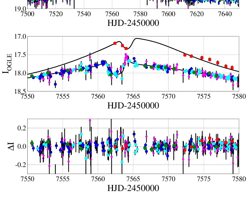
Figure 1: Light curve data of OGLE-2016-BLG-1067 (top panel), zoom around the anomaly (middle panel), and residual light curve (bottom panel). Spitzer and ground base data have square and circle symbols, respectively. The data from the different data sets are color coded. The model and the residual light curve are for the $\pi_{\mathrm{E,-,-}}$-large-$s$ solution, the best model according to the $\chi^{2}$ hierarchy (Table 1) with $\chi^{2}$/dof=2562/2545.

The microlensing program with Spitzer for 2016, Cycle 12 of the warm mission (Storrie-Lombardi & Dodd, 2010), was awarded a total of 300 hours (Gould et al., 2015a, b). One part of the project was specifically devoted to the follow up of events in the K2C9 footprint (Henderson et al., 2016). The larger part of the time was allocated with the aim of determining the Galactic distribution of planets (Calchi Novati et al., 2015a; Zhu et al., 2017a). OGLE-2016-BLG-1067 is located outside of the K2C9 footprint and therefore its selection followed the rules dictated by the “Criteria for Sample Selection to Maximize Planet Sensitivity and Yield from Space-Based Microlens Parallax Surveys” (Yee et al., 2015). We recall that, on a weekly basis, the list of the events to be followed up is finalized 4 days prior to the beginning of the observational sequence (Figure 1 from Udalski et al. 2015). Yee et al. (2015) defined a set of criteria for selecting events, and the corresponding observing strategy, according to which they may (or may not) be included in the sample of events for building up the statistics for determining the Galactic distribution of planets. These criteria allow events to be selected “objectively” (if they meet some pre-defined criteria), “subjectively” (at the discretion of the team), or “secretly”. “Objective” events must be observed by Spitzer. Therefore, planets detected in these events are included in the Galactic-distribution sample regardless of whether they give rise to signatures before or after the time they meet these criteria. See for example the analysis by Ryu et al. (2017) of OGLE-2016-BLG-1190. “Subjective” events must be publicly announced, together with a complete specification of the observation plan. Hence, planets that give rise to signatures in data that are available prior to this announcement cannot be included in the sample. For this reason, it is also possible to choose events “secretly”, in case it is unknown whether the event will be promising (and so worth extended Spitzer observations) at the time of the Spitzer upload. In this case, the event may subsequently be announced as a “subjective” event (with public commitment to carry out extended observations), or dropped. In the latter case, the planets discovered in the event prior to announcement cannot be included in the sample.

OGLE-2016-BLG-1067 fell in the last category. It was chosen “secretly” for the first week of Spitzer observations. Because it lay far to the East, the Spitzer Sun-angle restrictions prevented it from being observed until near the end of that week, so that only 3 observations were made. By the decision time for the second week, it appeared that the event was turning over at low magnification and so was dropped without making a “subjective” announcement. However, on June 24 UT 16:20, the MOA group announced an anomaly in this event based on their real-time data analysis. Based on this, it was decided to resume observations (after a 1-week hiatus), although it was recognized that the planet could not be included in the sample.

In order to verify the team’s original assessment that the planet could not be included in the Galactic-distribution sample, it is necessary to determine whether the decision to stop observations (rather than select the event “subjectively”) was influenced by the presence of the planet. That is, just as planets cannot be included in the sample if the decision to observe them is influenced by the presence of the planet, they equally cannot be excluded from the sample if the decision to stop observations is made due to its presence. This is a concern in the present case because the planet was first recognized from a dip in the light curve. Such a dip could in principle have been misinterpreted by the team as the event “turning over”. Hence, we reviewed the decision process quite carefully. We find that the decision was made based on data ${\rm HJD}^{\prime}\leq 7557.644$, i.e., roughly 4 days before the onset of the “dip” that led to the MOA alert. The effect of the planet on the magnification profile during these earlier observations is far below the observational error bars. Therefore, we conclude that the presence of the planet did not in any way influence the team’s decision.

Overall we have obtained 25 “epochs” of Spitzer data, on average 1 each 24 hours, except during the one-week gap after the first 3 data points. Each epoch is composed by six $30~{}\mathrm{s}$ dithered exposures. For the observations we use the $3.6~{}{\mu}\mathrm{m}$ channel 1 of the IRAC camera (Fazio et al., 2004). The data reduction follows the specific pipeline described in Calchi Novati et al. (2015b).

3 Light Curve Analysis

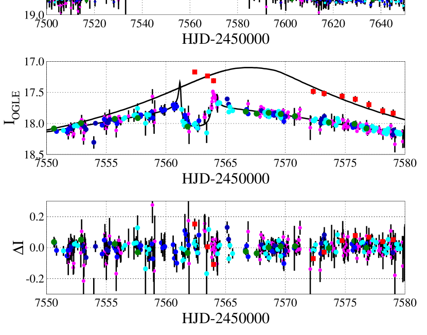
Figure 2: Light curve data of OGLE-2016-BLG-1067 (top panel), zoom around the anomaly (middle panel), and residual light curve (bottom panel). Spitzer and ground base data have square and circle symbols, respectively. The data from the different data sets are color coded. The model and the residual light curves are for the $\pi_{\mathrm{E,+,-}}$-small-$s$ solution, the worst model according to the $\chi^{2}$ hierarchy (Table 2) with $\chi^{2}$/dof=2591/2545.

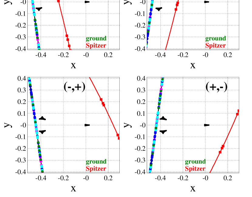
Figure 3: The caustic curves and the source trajectory in the lens plane as seen from ground and from Spitzer for the four large-$s$ solutions (Table 1). Spitzer and ground base data have square and circle symbols, respectively. The data from the different data sets are color coded as in Figure 1 and Figure 2.

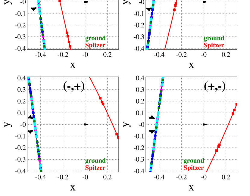
Figure 4: The caustic curves and the source trajectory in the lens plane as seen from ground and from Spitzer for the four small-$s$ solutions (Table 2). Spitzer and ground base data have square and circle symbols, respectively. The data from the different data sets are color coded as in Figure 1 and Figure 2.

The light curve of the event mostly follows a single-lens model except for a deviation occurring at about peak magnification. The single-lens model indicates a low magnification event that is punctuated by a short dip (Figures 1 and 2), which is the classic signature of a “minor image” perturbation due to a planet. The host star gives rise to two images, which according to Fermat’s principle are at stationary points of the time-delay surface. The smaller of these two images is at a saddle point and so can easily be annihilated if a planet lies at or close to this position. The ratio of the unperturbed magnification of these two images is $(A-1)/(A+1)$, where $A$ is the total magnification. Hence for a low-magnification $A_{\rm max}\sim 2.5$ event such as this one, at most a fraction $\sim 30\%$ of the flux can be eliminated. Moreover, the point where the flux is most strongly suppressed is flanked by two triangular caustics; however, the light curve does not exhibit any caustic crossings. Rather, it shows signs of cusp approaches just before and after the “dip”. Hence, we conclude that the source has passed close to, but has not intersected the two caustics that flank the dip in the magnification profile. This introduces a potential degeneracy with the source trajectory passing on either side on the planetary caustics with respect to the central caustic (Figures 3 and 4).

The microlensing magnification $A(t)$ for a single lens is, in the standard Paczyński (1986) form, a function of three parameters: the time of maximum magnification, $t_{0}$, the impact parameter, $u_{0}$, and the Einstein time, $t_{\mathrm{E}}$. Additionally, the effect of finite source size is parameterized by $\rho=\theta_{*}/\theta_{\mathrm{E}}$, where $\theta_{*}$ is the angular source size and $\theta_{\mathrm{E}}$ is the Einstein angular radius. To model a binary lens system we introduce three additional parameters: the mass ratio between the planet and its host star, $q$, their instantaneous projected separation, in units of the Einstein radius, $s$, and an angle specifying the source trajectory with respect to the binary axis, $\alpha$. In addition to this set of seven non-linear parameters, for a given model, there are two flux parameters, the source flux, $f_{s}$, and the blend, $f_{b}$, for each data set, entering linearly in the magnification model, $f(t)=f_{b}+f_{s}\cdot A(t)$.

From the observed ground-based light curve we may obtain a first guess on the values of the binary parameters based on the single lens model, for which $u_{0}\sim 0.4$ and $t_{\mathrm{E}}\sim 30~{}\mathrm{d}$, and the expected planetary model. Because of the absence of a caustic crossing and the anomaly occurring at about the peak magnification we expect $u_{0}=s-1/s$, giving the pair of solutions $s\sim 0.8$ and $s\sim 1.2$. The anomaly shape, a clear dip, indicates without ambiguity that only the first, close, solution is viable. For a trajectory approximately perpendicular to the binary axis, $\Delta t/t_{\mathrm{E}}\sim 2\eta_{c,0}$, where $\eta_{c,0}\simeq 2\sqrt{q}/s\cdot(1-0.5\,s^{2})$ is the position of the planetary caustic along the axis perpendicular to the binary axis (Han, 2006), and $\Delta t$ is the dip duration. For $\Delta t\sim 3~{}\mathrm{day}$ we evaluate therefore $q\sim 10^{-3}$. We note that this is the same preferred solution as in the Real-Time Microlensing Modeling by V. Bozza, which is the result of a completely independent and automated search algorithm across the full parameter space. (Comparing to the real-time models by V. Bozza, we note that these did not include KMTNet data. In the present analysis the dip, and therefore the solution with $s<1$, is much better constrained because of the dense coverage ensured by these data.)

In addition to the basic lensing parameters, the simultaneous observations from space with Spitzer allow us to constrain the microlensing parallax, which we parameterize with the two components along the North and East axes, $\pi_{\mathrm{E,N}},\,\pi_{\mathrm{E,E}}$ (Gould, 2004). For two fixed observers, the microlensing parallax is affected by a four-fold degeneracy (Refsdal, 1966; Gould, 1994), which in principle can be removed in the case of binary lens systems (as in the case of OGLE-2015-BLG-1212, Bozza et al. 2016). As we detail below however, also because of the gap in Spitzer data, we are unable to conclusively break this degeneracy from light-curve modeling alone. To constrain the microlens parallax with the simultaneous fit of ground and space-based data, we follow Gould (2004) using in particular the known position of Spitzer relative to Earth as a function of time from the Horizons Ephemeris System.

We search for the best model in the parameter space through $\chi^{2}$ minimization (for Spitzer we add a penalty term related to a constraint on the flux that we obtain from color-color regression, see below). To this purpose, as well as for the determination of the uncertainties on the parameters, we make use of a Markov chain Monte Carlo (MCMC), which we seed according to the heuristic analysis presented above. For the modeling we proceed in the geocentric frame (with $t_{0,\mathrm{par}}=7564$, i.e., about the time of maximum magnification). In order to evaluate the microlensing magnification given the model, we make use of a combination of codes: the contour integration (Gould & Gaucherel, 1997) as developed by Bozza (2010) and recently released to the public, in the anomaly region, and hexadecapole, quadrupole or monopole approximations (Pejcha & Heyrovský, 2009; Gould, 2008) elsewhere. For the finite source size we adopt (Yoo et al., 2004) linear limb darkening coefficients $\Gamma_{R,\mathrm{MOA}}=0.494$ (estimated out of the average of $\Gamma_{R}$ and $\Gamma_{I}$), $\Gamma_{I}=0.410$ and $\Gamma_{L}=0.144$ based on the source characterization described below and the model of Claret & Bloemen (2011). However, the lack of caustic crossings make the results only weakly dependent on these parameters.

As mentioned, the flux parameters (source and blend flux for each data set) enter the magnification model linearly. It is therefore common practice to fit for them analytically within the MCMC after the non-linear parameters are fixed in each trial. This increases the speed but comes at the price of losing the information of possible covariance terms from their cross-correlation with the non-linear parameters. As an exception, here we consider the Spitzer flux parameters as chain parameters, which thereby allows us a more reliable characterization of the $(R_{\mathrm{MOA}}-L)$ color, which is crucial for comparison to the color-color based constraint.

A preliminary analysis with the MCMC confirms the initial assessment of the lack of caustic crossings and in particular, as discussed in Section 1, the impossibility to measure the Einstein angular radius, $\theta_{\mathrm{E}}$, based on the light curve analysis of the finite source size effect, $\rho$, together with the characterization of the source size, $\theta_{*}$ (Equation (2) and Equation (3)). More specifically, we can only establish an upper limit for $\rho$, which in turn can be translated, given the parallax measurement, into a lower limit on the lens mass and an upper limit on its distance. We further explore this line of reasoning in the following sections devoted to the analysis of the physical parameters of the lens system. (It is worth recalling that with particular geometry configurations, as for OGLE-2016-BLG-1195Lb (Bond et al., 2017; Shvartzvald et al., 2017), it is indeed possible to obtain a clear measurement of the finite source parameter, $\rho$, even in absence of caustic crossings.)

Table 1: All solutions (“large”-$s$)

Parameters	small $\pi_{\rm E}$		large $\pi_{\rm E}$
$\chi^{2}$/dof	2561/2545	2567/2545	2573/2545	2589/2545
	$(-,-)$	$(+,+)$	$(-,+)$	$(+,-)$
$t_{0}$ [HJD-2457564.]	$0.325_{-0.064}^{+0.065}$	$0.300_{-0.063}^{+0.065}$	$0.308_{-0.065}^{+0.065}$	$0.241_{-0.066}^{+0.065}$
$u_{0}$	$-0.470_{-0.029}^{+0.029}$	$0.474_{-0.029}^{+0.030}$	$-0.451_{-0.034}^{+0.031}$	$0.444_{-0.030}^{+0.032}$
$t_{\mathrm{E}}$ [days]	$26.5_{-1.1}^{+1.2}$	$26.4_{-1.1}^{+1.2}$	$27.2_{-1.3}^{+1.3}$	$27.5_{-1.3}^{+1.3}$
$\rho$ [$10^{-3}$]	$<5.5$	$<5.8$	$<5.9$	$<5.2$
$\pi_{\mathrm{E,N}}$	$0.220_{-0.014}^{+0.015}$	$-0.223_{-0.015}^{+0.014}$	$0.620_{-0.048}^{+0.052}$	$-0.635_{-0.051}^{+0.048}$
$\pi_{\mathrm{E,E}}$	$-0.054_{-0.008}^{+0.006}$	$-0.010_{-0.008}^{+0.007}$	$-0.204_{-0.017}^{+0.015}$	$-0.085_{-0.010}^{+0.009}$
$\alpha$ [rad]	$1.427_{-0.006}^{+0.006}$	$4.854_{-0.006}^{+0.006}$	$1.426_{-0.006}^{+0.006}$	$4.853_{-0.006}^{+0.007}$
$s$	$0.812_{-0.012}^{+0.012}$	$0.811_{-0.012}^{+0.012}$	$0.820_{-0.014}^{+0.014}$	$0.824_{-0.014}^{+0.013}$
$q$ [$10^{-3}$]	$1.460_{-0.055}^{+0.063}$	$1.462_{-0.054}^{+0.065}$	$1.463_{-0.054}^{+0.063}$	$1.467_{-0.054}^{+0.062}$
$f_{\mathrm{s,OGLE}}$	$0.516_{-0.045}^{+0.049}$	$0.522_{-0.046}^{+0.050}$	$0.486_{-0.047}^{+0.054}$	$0.476_{-0.045}^{+0.051}$
$f_{\mathrm{b,OGLE}}$	$0.030_{-0.048}^{+0.045}$	$0.024_{-0.050}^{+0.046}$	$0.059_{-0.054}^{+0.047}$	$0.069_{-0.050}^{+0.045}$
$R_{\mathrm{MOA}}-L_{Spitzer}$	$1.131_{-0.050}^{+0.050}$	$1.150_{-0.050}^{+0.049}$	$1.110_{-0.059}^{+0.059}$	$1.122_{-0.060}^{+0.060}$
$\theta_{*}$ [$\mu$as]	$0.851_{-0.038}^{+0.039}$	$0.856_{-0.038}^{+0.040}$	$0.826_{-0.041}^{+0.045}$	$0.817_{-0.040}^{+0.042}$

Table 2: All solutions (“small”-$s$)

Parameters	small $\pi_{\rm E}$		large $\pi_{\rm E}$
$\chi^{2}$/dof	2566/2545	2572/2545	2575/2545	2590/2545
	$(-,-)$	$(+,+)$	$(-,+)$	$(+,-)$
$t_{0}$ [HJD-2457564.]	$0.312_{-0.063}^{+0.063}$	$0.289_{-0.062}^{+0.062}$	$0.300_{-0.062}^{+0.064}$	$0.231_{-0.062}^{+0.063}$
$u_{0}$	$-0.442_{-0.031}^{+0.029}$	$0.442_{-0.029}^{+0.031}$	$-0.444_{-0.033}^{+0.031}$	$0.440_{-0.030}^{+0.033}$
$t_{\mathrm{E}}$ [days]	$27.6_{-1.2}^{+1.3}$	$27.5_{-1.2}^{+1.3}$	$27.4_{-1.3}^{+1.3}$	$27.6_{-1.3}^{+1.3}$
$\rho$ [$10^{-3}$]	$<4.8$	$<4.7$	$<4.9$	$<4.4$
$\pi_{\mathrm{E,N}}$	$0.196_{-0.016}^{+0.016}$	$-0.198_{-0.017}^{+0.015}$	$0.611_{-0.047}^{+0.050}$	$-0.629_{-0.052}^{+0.048}$
$\pi_{\mathrm{E,E}}$	$-0.054_{-0.009}^{+0.008}$	$-0.015_{-0.009}^{+0.008}$	$-0.202_{-0.016}^{+0.015}$	$-0.085_{-0.010}^{+0.010}$
$\alpha$ [rad]	$1.430_{-0.006}^{+0.006}$	$4.851_{-0.006}^{+0.006}$	$1.431_{-0.006}^{+0.006}$	$4.847_{-0.006}^{+0.006}$
$s$	$0.785_{-0.011}^{+0.010}$	$0.785_{-0.011}^{+0.010}$	$0.784_{-0.012}^{+0.011}$	$0.786_{-0.012}^{+0.011}$
$q$ [$10^{-3}$]	$1.317_{-0.031}^{+0.033}$	$1.321_{-0.032}^{+0.032}$	$1.322_{-0.031}^{+0.032}$	$1.332_{-0.032}^{+0.034}$
$f_{\mathrm{s,OGLE}}$	$0.473_{-0.043}^{+0.049}$	$0.474_{-0.044}^{+0.049}$	$0.478_{-0.046}^{+0.052}$	$0.471_{-0.045}^{+0.052}$
$f_{\mathrm{b,OGLE}}$	$0.072_{-0.049}^{+0.043}$	$0.071_{-0.049}^{+0.043}$	$0.067_{-0.051}^{+0.046}$	$0.074_{-0.052}^{+0.044}$
$R_{\mathrm{MOA}}-L_{Spitzer}$	$1.166_{-0.056}^{+0.055}$	$1.186_{-0.055}^{+0.054}$	$1.115_{-0.060}^{+0.059}$	$1.123_{-0.060}^{+0.062}$
$\theta_{*}$ [$\mu$as]	$0.815_{-0.038}^{+0.041}$	$0.816_{-0.038}^{+0.041}$	$0.819_{-0.041}^{+0.043}$	$0.813_{-0.040}^{+0.044}$

Overall we find $(2\times 4)=8$ competitive event geometries, which are the product of the two degeneracies anticipated above. The first degeneracy is driven by ground-based data, with a larger (smaller) value for $s$ for the source trajectory passing outside (inside) the planetary caustics, with respect to the central caustic, with values about $0.81-0.82$ and $0.78-0.79$, respectively. (More precisely, the degeneracy occurs in the $s,q$ parameter space, with $q\sim 1.5\times 10^{-3}$ and $1.3\times 10^{-3}$ in the two cases, respectively). In the second model, the first sharp cusp approach falls in a gap of the data whereas both cusp approaches are well sampled for the first model. For each of these two possible source trajectories, as seen from the ground, we then have the four viable degenerate microlensing parallax solutions compatible with the data, i.e., the two-fold degeneracy for the microlensing parallax amplitude, $\pi_{\mathrm{E,-}}\sim 0.2$ and $\pi_{\mathrm{E,+}}\sim 0.6$ (the $(-,-)$, $(+,+)$ and $(-,+)$, $(+,-)$ solutions respectively). For the first solution, $\pi_{\mathrm{E,-}}$, the source trajectory as seen from Spitzer passes in between the central caustic and the planetary caustics, and near enough to the latter to show a deviation from the smooth single lens shape. In the second solution, $\pi_{\mathrm{E,+}}$, the trajectory passes far away from all the caustics. Although the first three data points along the Spitzer light curve before the gap hint at a non-Paczyński shape, by themselves they are not sufficient to unambiguously resolve the degeneracy.

In Tables 1 and 2, we report for each of the eight solutions (for the outer and inner ground-based source trajectory, respectively, to which we will hereafter refer as “large” and “small”-$s$) the minimum $\chi^{2}$, the best (median) value and the corresponding 16%-84% ranges of the non-linear parameters of the magnification model, the OGLE flux parameters and the $(R_{\mathrm{MOA}}-L)$ color. As discussed, the model can not constrain $\rho$, and we report a $3\,\sigma$ upper limit. In addition, we also report the MCMC outcome for the angular source radius, which is a derived quantity based on the model-independent prior knowledge of the source color (see Section 4.1). The $\chi^{2}$ difference does not break the degeneracy in the $s$ parameter space. Indeed, for each pair of degenerate microlensing parallax solutions, $\Delta\chi^{2}$ is at most $\sim 5$, although the large-$s$ solution is systematically favored. As for the microlensing parallax degeneracy, the $\pi_{\mathrm{E,-}}$ solutions have smaller $\chi^{2}$. For both $s$ cases, the $\chi^{2}$ hierarchy is $(-,-),\,(+,+),\,(-,+),\,(+,-)$ with $\Delta\chi^{2}\sim 6,\,12,\,28$ ($\Delta\chi^{2}\sim 6,\,9,\,24$) for the large (small)-$s$ solution, respectively, with the hierarchy being driven by the Spitzer data and only the $(+,-)$ solution clearly disfavored. The features of the different magnification models are driven by the microlens parallax for Spitzer, whereas for the ground-based observations, they are driven by the $(s,\,q)$ pair. The $\pi_{\mathrm{E,-}}$ solutions have the peak magnitication occuring earlier and showing, although smoothed, the same anomaly seen from ground. The solutions with large $s$ have, from ground, both cusp approaches very well sampled by the available data, whereas those with small $s$ have the first, sharper, cusp approach falling in a gap of the data. Finally, each pair of solutions that differ by the inversion $u_{0}\to-u_{0}$ is qualitatively indistinguishable. In Figures 1 and 2, we show the light curve for both ground and Spitzer data, together with the corresponding model and the residuals for the $(-,-)$-large-$s$ and the $(+,-)$-small-$s$ solutions. These two light curves therefore show, at least qualitatively, the full range of possible configurations. At the same time they are, respectively, the best and the worst ones according to the $\chi^{2}$ hierarchy. The caustic structure and the source trajectories, as seen from the ground and from Spitzer, are shown for all eight solutions in Figures 3 and 4. An additional analysis of Tables 1 and 2 reveals that except for the degenerate parameters in the corresponding degenerate solutions, $s,\,q,\,u_{0},\,\pi_{E,N},\,\pi_{E,E}$ and $\alpha$, the MCMC parameters for all the solutions , are compatible with one another at 68% level. Additionally, the pair $(s,\,q)$ even for the degenerate solutions are still compatible at the 90% level. Apart from the $\rho$ parameter, for each configuration the model is very well constrained. The binary lens topology is extremely well determined, with relative error about $2\%$ and $4\%$ in $s$ and $q$, respectively, and the error of the trajectory angle is $<0.5^{\circ}$. The relative error in the microlensing parallax is at most about $8\%$ and is about $5\%$ and $7\%$ for $t_{\rm E}$ and $u_{0}$, respectively.

4 Characterization of Source and Lens Fluxes

In this Section we carry out the photometric analysis of the source and discuss the limit that we can put on the lens flux based on the microlens modeling.

4.1 Color-Magnitude Diagram

The light curve microlensing model gives us the values for the source and the blend flux. Additionally, independently from the microlensing model, we can evaluate the source color. By combining this information with the analysis of the color-magnitude diagram (CMD), we can characterize the source, specifically obtain its angular radius, and, comparing to the blend, obtain an upper limit for the lens flux. Finally, cross-matching the optical and the Spitzer CMDs we can evaluate, again independently from the light curve model, a color-constraint between the ground-based and the Spitzer flux, which we can then use within the light curve modeling. (This is necessary to account for the incomplete coverage of the underlying primary microlensing event with Spitzer data, Calchi Novati et al. 2015a; Zhu et al. 2017a).

Following Yoo et al. (2004), the key in the color analysis, with the purpose to obtain the source dereddened color and magnitude, is the study of the offset of the measured to the intrinsic centroid of the “red giant clump”. For the latter we have $(V-I,I)_{\mathrm{cl,0}}=(1.06,14.31)$ (Bensby et al., 2013; Nataf et al., 2013). For the first, and for the overall source color analysis, we rely on the MOA and OGLE data.

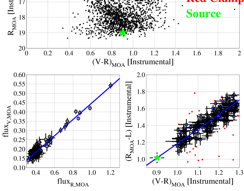
Figure 5: Top panel: MOA instrumental CMD of stars centered on the event position. The positions of the red clump centroid (filled circle) and of the source are indicated. Bottom left panel: MOA $V$ versus $R_{\mathrm{MOA}}$ flux for the source color analysis. The solid line shows the best fit linear model color solution. Here and in the bottom panel the red dots, without error bars, indicates the values iteratively rejected within the fit procedure. Bottom right panel: Instrumental MOA and Spitzer $(R_{\mathrm{MOA}}-L)$ vs $(V-R)_{\mathrm{MOA}}$ and best fit linear model. For the given value of the $(V-R)_{\mathrm{MOA}}$ source color, obtained from the data alone (therefore model-independent), the star indicates the position of the resulting $(R_{\mathrm{MOA}}-L)$.

We start by building the CMD with stars centered on the event position based on instrumental $V$-band and $R_{\mathrm{MOA}}$-band magnitudes. See Figure 5 (top panel). In particular following the DIA alignment procedure presented by Bond et al. (2017), we measure the instrumental color $(V-R)_{\mathrm{cl,MOA}}=1.195\pm 0.015$, which we translate, using the MOA calibration to the OGLE-III database (Szymański et al., 2011), to $(V-I)_{\mathrm{cl}}=1.766\pm 0.016$. Based on the light curve data, we determine the source color from regression of MOA-$V$ versus MOA-$R$ flux as the source magnification changes (Figure 5, middle panel). It is relevant to recall that this determination is independent from the light curve modeling. By correcting for the clump offset we obtain $(V-I)_{\mathrm{s,0}}=0.742\pm 0.035$.

Next, we consider the EWS OGLE-IV CMD for which we evaluate $I_{\mathrm{cl,OGLE-IV}}=15.110$. The resulting source magnitude, as inferred from the microlensing model, is given in Tables 1 and 2, where the OGLE source and blend flux values have a magnitude zero-point of 18. Assuming that the source lies behind the same column of dust as the red clump, we obtain for the (preferred) $(-,-)$ solutions, $I_{\mathrm{OGLE},0}=17.92\pm 0.10$ and $I_{\mathrm{OGLE},0}=18.01\pm 0.10$ for the large-s and small-$s$ geometries, respectively. Overall, based on its position in the CMD, the source appears to be a G5-G6 dwarf. As already mentioned in Section 3, in the analysis to establish the upper limit on the lens flux based on the measured blend flux, we also conservatively assume the lens to be behind the same column of dust as the red clump.

Combining these results, moving from $(V-I,I)$ to $(V-K,K)$ by means of standard color relations (Bessell & Brett, 1988) and using the relation between color and surface brightness (Kervella et al., 2004), we can finally estimate $\theta_{*}$, which spans the range of values $0.81-0.86\,\mu\mathrm{as}$ for the different models (via the source flux).

Finally, we can use the source color to constrain the Spitzer instrumental flux relative to the ground-based one. Specifically, cross-matching the MOA CMD to Spitzer field stars we establish a $(VR)_{\mathrm{MOA}}L_{Spitzer}$ color-color relation. See the bottom panel of Figure 5. Specifically, given the source instrumental color, we obtain $(R_{\mathrm{MOA}}-L_{Spitzer})=1.018\pm 0.063$ from linear regression of a sample of stars representative of the bulge population chosen around the clump position. As is the case for the source color, this determination is also independent of the light curve model.

4.2 Limit on the Lens Flux

As discussed in Section 3, the lack of caustic crossings in the lens geometry renders impossible the measurement of the source size parameter, $\rho$. This propagates to the measurement of the Einstein angular radius $\theta_{\rm E}=\theta_{*}/\rho$ and eventually to the determination of the lens parameters. (Rather, we obtained only an upper limit on $\rho$, and thus a lower limit on $\theta_{\rm E}=\theta_{*}/\rho$.) We can, however, combine the measurement of the microlens parallax $\pi_{\rm E}$ with an upper limit on the lens flux, to indirectly obtain an upper limit on $\theta_{\rm E}$ (Udalski et al., 2015) (see also the more general analysis of Yee 2015). That is, if $\pi_{\rm E}$ is known, then increasing $\theta_{\rm E}$ leads to both more massive ($M=\theta_{\rm E}/\kappa\pi_{\rm E}$) and closer ($\pi_{\rm rel}=\theta_{\rm E}\pi_{\rm E}$) lenses, whose inferred flux eventually exceeds the limits on lens flux set by the blended light. This upper limit on $\theta_{\rm E}$ can also be thought of as a lower limit on $\rho=\theta_{*}/\theta_{\rm E}$. This procedure is in principle always possible. However, in order to be effective it must happen, as is the case here, that the blend be faint enough so as to obtain a meaningful limit.

We are going to exploit this possibility in the simulation that we carry out to include the Galactic model in the determination of the physical parameters, Section 5.1.3. Given the lens mass and distance, based on a mass-luminosity relation (Baraffe & Chabrier, 1996), we can estimate the corresponding lens magnitude, which we can then compare with the (OGLE-based) blend magnitude given by the microlensing model. Accordingly, we eliminate too close, too bright lenses corresponding to, for a given source angular size, increasingly low values of $\rho$.

For reference, the threshold magnitude based on the blend flux, taking into account the extinction, is about $I\sim 19.5$, and for a distance of $1,\,2,\,4$ and $6\,\mathrm{kpc}$ this corresponds to a maximum mass of $0.25,\,0.48,\,0.68$ and $0.80\,\mathrm{M_{\odot}}$, respectively.

5 A Sub-Jupiter Mass Planet Beyond the Snow Line

With a planet to host mass ratio of about $q\simeq 1.3-1.5\times\,10^{-3}$, the light curve modeling suggests, most likely, a sub-Jupiter mass planet. However, because $\theta_{\rm E}$ is only weakly constrained, and because there are eight different possible topologies (comprised of two groups with substantially different values of $\pi_{\rm E}$), we cannot translate these results into an estimate of physical parameters based on the microlensing light curve alone.

We now seek to resolve and/or tighten all these degeneracies, both continuous and discrete, by combining four types of parameter measurements/constraints and three arguments. The parameter measurements/constraints are:

1. (1) Well-measured microlens parameters $(t_{\rm E},\pi_{{\rm E},N},\pi_{{\rm E},E},q,s)$ from the MCMC

2. (2) Function $\Delta\chi^{2}(\rho)$ derived from the MCMC

3. (3) Measurement of $\theta_{*}$

4. (4) Flux constraint, as described in Section 4.2.

The arguments are discussed in detail in Section 5.1 and are

1. (1) $\chi^{2}$ hierarchy

2. (2) “Rich argument”

3. (3) Galactic model

5.1 Resolution of the Degeneracies I: Framework

As discussed in Section 3 and tabulated in Tables 1 and 2, there is a $(2\times 4)=8$ fold degeneracy of solutions that need to at least be considered. In fact, these degeneracies can be further subdivided (and re-ordered) as a $(2\times 2\times 2)=8$ product of ($\pi_{{\rm E},+}$ vs. $\pi_{{\rm E},-}$)$\times$($\pi_{{\rm E},N}>0$ vs. $\pi_{{\rm E},N}<0$) $\times$($s_{\rm small}$ vs. $s_{\rm large}$). This ordering reflects both the relative importance of the degeneracies in terms of physical implications for the system and (happily) the ease with which they are broken.

To break these degeneracies, we consider three independent pieces of evidence: 1) $\chi^{2}$ of the best model for each local minimum, 2) “Rich argument”, and 3) Bayesian inference based on a Galactic model. We specifically evaluate to what extent these separate pieces of evidence support and/or contradict one another.

We begin by assuming that, in the absence of any other consideration, each of the eight separate minimum should be considered equally likely to be the location of the correct solution.

5.1.1 $\chi^{2}$ hierarchy

The values of $\chi^{2}$ for each of the eight minima are given in Tables 1 and 2. Since, each model contains the same number of dof, the nominal relative probability of these models is simply $\exp(-\Delta\chi^{2}/2)$. However, first, some of the models differ by only $\Delta\chi^{2}=3$ and even those with fundamentally different physical implications can differ by only $\Delta\chi^{2}=6$. Thus, even taken at face value, the $\chi^{2}$ differences do not decisively distinguish between solutions. Second, it is well known that microlensing light curves can have low-level systematics that generate spurious $\chi^{2}$ differences at these levels. Thus, depending on the specific $\chi^{2}$ differences between alternate solutions, additional arguments may be needed to distinguish between them.

5.1.2 “Rich Argument”

The “Rich argument” (Calchi Novati et al., 2015a) states that, other things being equal, small parallax solutions are preferred over large ones by a factor $(\pi_{{\rm E},+}/\pi_{{\rm E},-})^{2}$, which, for the case we will consider below, yields $(\pi_{{\rm E},+}/\pi_{{\rm E},-})^{2}\simeq 10$. The reason is that if the true parallax is small, it will generically give rise to a large-parallax alternate-degenerate solution, but if the true parallax is large, it will give rise to a small-parallax alternate solution with only $(\pi_{{\rm E},-}/\pi_{{\rm E},+})^{2}$ probability. Of course, “all other things” may not “be equal”. For example, in the case of the very massive planet OGLE-2016-BLG-1190Lb (Ryu et al., 2017), it was conclusively demonstrated, using two independent supplementary arguments, that the large parallax solution was correct. However, in that case, the balance of evidence favored the larte-parallax solution even in the absence of supplementary arguments. First, for OGLE-2016-BLG-1190Lb, the “Rich-argument” preference was much smaller, only 2.7 compared to the value that we will derive below, 10. Second, $\chi^{2}$ actually favored the large parallax solution by $\Delta\chi^{2}=13$ (and $\Delta\chi^{2}$ was not one of the independent arguments).

The key point is that, in contrast to the $\Delta\chi^{2}$ argument, which could in principle be subject to systematic errors, the “Rich argument” is purely statistical in nature, and its resulting probability ratio must be taken at face value.

5.1.3 Galactic Model

If the model fitting had resulted in unambiguous measurements of ${\mbox{\boldmath$\pi$}}_{\rm E}$ and $\rho$, then these would yield $\theta_{\rm E}=\theta_{*}/\rho$ (since we were able to measure $\theta_{*}$ in Section 4.1), and so also $M=\theta_{\rm E}/\kappa\pi_{\rm E}$ and $\pi_{\rm rel}=\theta_{\rm E}\pi_{\rm E}$. Then, because the source distance $D_{S}\simeq 7.66\,\mathrm{kpc}$ is also reasonably well known, there would be no need for a Galactic model.

Unfortunately, $\rho$ is not actually measured (although it is constrained in the sense that increasingly larger values of $\rho$ yield progressively worse $\chi^{2}$), while the measurement of ${\mbox{\boldmath$\pi$}}_{\rm E}$ suffers from the traditional four-fold degeneracy, including a two-fold ambiguity in its amplitude, $\pi_{\rm E}$.

Nevertheless, the information that we do have 1) precise (albeit four-fold degenerate) measurements of ${\mbox{\boldmath$\pi$}}_{\rm E}$, 2) precise measurement of $t_{\rm E}$, 3) constraints (albeit weak) on $\rho$, and 4) constraints on blended light, together act as powerful constraints on the Galactic model.

For each of the eight solutions, we begin by extracting from the MCMC the best fit $a_{0,i}$ and covariance $c_{ij}$ of the three measured quantities $a_{i}=(\tilde{v}_{{\rm hel},N},\tilde{v}_{{\rm hel},E},t_{\rm E})$. Here

$$\tilde{\mbox{\boldmath$v$}}_{\rm hel}=\tilde{\mbox{\boldmath$v$}}_{\rm geo}+\mbox{\boldmath$v_{\oplus,\perp}$}={{\mbox{\boldmath$\pi$}}_{\rm E}{\rm au}\over\pi_{\rm E}^{2}t_{\rm E}}+\mbox{\boldmath$v_{\oplus,\perp}$}$$ (4)

where ${\mbox{\boldmath$v$}}_{\oplus,\perp}(N,E)=(0.6,29.3)\,{\rm km}\,{\rm s}^{-1}$ is Earth’s velocity projected on the plane of the sky.

As we describe below, these measurements (together with the constraints on $\rho$) already rule out bulge lenses. We therefore consider disk lenses drawn according to a Han & Gould (1995) model (except with rotational velocity $v_{\rm rot}=235\,{\rm km}\,{\rm s}^{-1}$) and source distance $D_{S}=7.66\,{\rm kpc}$ (and specifically with the distance drawn according to $D_{l}^{2}\cdot\rho(D_{l})$, where $\rho(D_{l})$ is the spatial distribution along the given line of sight). For each simulated event, we draw a mass randomly from a Kroupa (2001) mass function. We then calculate the resulting $\theta_{\rm E}=\sqrt{\kappa M\pi_{\rm rel}}$, $\tilde{\mbox{\boldmath$v$}}_{\rm hel}={\mbox{\boldmath$\mu$}}_{\rm hel}{\rm au}/\pi_{\rm rel}$, $\tilde{\mbox{\boldmath$v$}}_{\rm geo}$ (from Equation (4)), $\mu_{\rm geo}=(\tilde{v}_{\rm geo}/\tilde{v}_{\rm hel})\mu_{\rm hel}$, $t_{\rm E}=\theta_{\rm E}/\mu_{\rm geo}$, and $\rho=\theta_{*}/\theta_{\rm E}$. Using $D_{l}$, $M$ and a mass-luminosity relation from Baraffe & Chabrier (1996) (and a conservative assumption that the lens lies behind all the dust) we also calculate the $I$-band flux from the lens.

We then evaluate

$$\chi^{2}_{\rm gal}=\chi^{2}(\tilde{\mbox{\boldmath$v$}}_{\rm hel},t_{\rm E})+\Delta\chi^{2}(\rho);\qquad\chi^{2}(\tilde{\mbox{\boldmath$v$}}_{\rm hel},t_{\rm E})=\sum_{i,j=1}^{3}(a-a0)_{i}b_{ij}(a-a0)_{j},$$ (5)

where $a_{i}=(\tilde{v}_{{\rm hel},N},\tilde{v}_{{\rm hel},E},t_{\rm E})$ and $b\equiv c^{-1}$. Each trial in the MCMC gives a value of $\chi^{2}(\rho)$; the lower envelope of this distribution gives the minimum $\chi^{2}$ for a gievn value of $\rho$. Thus, we can construct a function $\Delta\chi^{2}(\rho)$ from $\min(\chi^{2}(\rho)|\rho)-\min(\chi^{2})$, to create a $\chi^{2}$ penalty that increases as the value of $\rho$. We count all trials, $N_{\rm trial}$, but tabulate only those that contribute significantly to the total likelihood ($\chi^{2}_{\rm gal}<20$), $N_{\rm tabul}$. We also exclude trials that fail the flux constraint (Section 4.2). We then calculate a mean likelihood as the sum of weights evaluated by combining $\chi^{2}_{\rm gal}$ and the microlensing rate contribution

$$\langle L\rangle={\sum_{i=1}^{N_{\rm tabul}}w_{i}\over N_{\rm trial}}\,,\quad w_{i}=\exp(-\chi^{2}_{{\rm gal},i}/2)\times\theta_{{\rm E},i}\,\mu_{{\rm geo},i}\,.$$ (6)

Of course, these mean likelihoods are very small in all cases. This simply reflects the fact that $a_{0,i}=(\tilde{v}_{{\rm hel},N},\tilde{v}_{{\rm hel},E},t_{\rm E})$ is well measured, which immediately “rules out” the overwhelming majority of random trials drawn from the Galactic model. However, the only matters of concern to us are 1) what is the relative likelihood between different solutions, 2) what are the parameters (and errors) of each solution, and 3) are the parameters of the most likely (or several most likely) solutions “reasonable”?

5.1.4 Summary of Three Types of Information

Table 3: Resolution of the Degeneracies: the 8 solutions

Parameter	$(-,-)$		$(+,+)$		$(-,+)$		$(+,-)$
	“large”-$s$	“small”-$s$	“large”-$s$	“small”-$s$	“large”-$s$	“small”-$s$	“large”-$s$	“small”-$s$
$\chi^{2}-\chi^{2}_{\mathrm{best}}$	0.0	5.2	6.5	11.1	11.7	14.0	27.8	29.5
$(\pi_{\rm E}/\pi_{{\rm E},{\rm smallest}})^{2}$	$1.30\pm 0.27$	$1.04\pm 0.23$	$1.26\pm 0.26$	1.00	$10.8\pm 2.4$	$10.5\pm 2.4$	$10.4\pm 2.3$	$10.2\pm 2.3$
$\langle L\rangle/\langle L\rangle_{\mathrm{best}}$	0.59	1.00	$9.5\,10^{-4}$	$2.1\,10^{-3}$	$6.5\,10^{-2}$	$6.4\,10^{-2}$	$1.9\,10^{-3}$	$2.0\,10^{-3}$

Table 3 summarizes the results of the three types of information for the eight solutions. For each degenerate solution, following the combined effect of the four-fold microlensing parallax degeneracy and the $(s,\,q)$ topology degeneracy, for which details can be obtained from Tables 1 and 2, we report: the difference of $\chi^{2}$ relative to the best model; the “Rich argument” ratio, i.e,, $(\pi_{\rm E}/\pi_{{\rm E},{\rm smallest}})^{2}$ relative to the smallest $\pi_{\rm E}$; and finally, the Galactic model likelihood ratio $\langle L\rangle/\langle L\rangle_{\rm best}$.

5.2 Resolution of the Degeneracies II: Application

We now discuss how these three types of information discriminate between the three degeneracies.

5.2.1 Small vs. Large Microlens Parallax

The small vs large parallax degeneracy is the degeneracy between the first two columns of Tables 1 and 2 and the last two columns of these tables. It is the only one of the three degeneracies that impacts the interpretation of the internal nature of the system in a major way. That is, since $\pi_{{\rm E},-}/\pi_{{\rm E},+}\sim 1/3$ and since all other parameters are very similar in these solutions, the inferred mass $M=\theta_{\rm E}/\kappa\pi_{\rm E}$ (or range of allowed masses) will be three times smaller in the first than the second.

As shown in Table 3, all three arguments significantly favor the small parallax solutions. First, the best small parallax solution is favored over the best large parallax solution by $\Delta\chi^{2}=12$. Second, of course, the “Rich argument” (by definition) favors the small parallax solution by a ratio 10. Third, the Galactic model likelihood ratio also favors this small parallax solution. From Table 3, we see that the best small parallax solution has higher mean likelihood than the best large-parallax solution by a factor 15. This is primarily because the large-parallax solutions have more-nearby lenses and hence lower accessible Galactic volume. Taken together, the three arguments very strongly favor the small parallax solutions.

5.2.2 Positive vs. Negative $\pi_{{\rm E},N}$

Within this small-parallax $(\pi_{{\rm E},-})$ class of solutions, the solutions with $\pi_{{\rm E},N}>0$ $(-,-)$ are favored over those with $\pi_{{\rm E},N}>0$ $(+,+)$ by just $\Delta\chi^{2}\simeq 6$. This would not be conclusive, even under the assumption of purely Gaussian statistics. However, the Galactic model very strongly favors the $\pi_{{\rm E},N}>0$ $(-,-)$ solution, by a factor over 400. It is instructive to track exactly why the Galactic model favors these solutions, in part because this process allows us to understand why these solutions are not merely “better” but also intrinsically “reasonable”.

The two classes of solutions have very similar amplitudes $\tilde{v}_{\rm hel}\sim 290\,{\rm km}\,{\rm s}^{-1}$ and differ primarily in direction. Before continuing, we note that this projected velocity corresponds to a heliocentric proper motion,

$$\mu_{\rm hel}={\tilde{v}_{\rm hel}\pi_{\rm rel}\over{\rm au}}=0.9\,{{\rm mas}\,{\rm yr}^{-1}}{\tilde{v}_{\rm hel}\over 290\,{\rm km}\,{\rm s}^{-1}}\,{\pi_{\rm rel}\over 0.015\,{\rm mas}}.$$ (7)

Since bulge-bulge lensing typically yields $\pi_{\rm rel}\sim 0.015\,{\rm mas}$, Equation (7) implies that the lens is not likely to be in the bulge. Typical proper motions of bulge stars are about $2.7\,{\rm mas}\,{\rm yr}^{-1}$ in each direction, so that for bulge-bulge lensing, the relative motion is $\mu\sim 4\,{\rm mas}\,{\rm yr}^{-1}$. Of course, for any particular event it can in principle be smaller, but the prior probability that it is smaller than some value scales $p\sim(\mu/4\,{\rm mas}\,{\rm yr}^{-1})^{3}$, which is quite small in the present case. Moreover, such low proper motions would require $\rho=\theta_{*}/(\mu t_{\rm E})=0.012(\mu/0.9\,{\rm mas}\,{\rm yr}^{-1})^{-1}$. However, $\rho>0.006$ is ruled out by the fit at least at the $3\,\sigma$ level. Thus, we do not explicitly consider bulge lenses.

Next, we rotate the projected velocity to Galactic coordinates and evaluate it in the frame of the Local Standard of Rest (LSR), by adding $(12,7){\rm km}\,{\rm s}^{-1}$ in the $(l,b)$ directions. We then find $\tilde{v}_{\rm lsr}(l,b)=(235,182)\,{\rm km}\,{\rm s}^{-1}$ and $\tilde{v}_{\rm lsr}(l,b)=(-233,-154)\,{\rm km}\,{\rm s}^{-1}$ for the two solutions. If all disk stars were on a flat rotation curve of velocity $v_{\rm rot}$, and all bulge stars were at rest with respect to the center of the Galaxy, we would expect $\tilde{v}_{\rm lsr}(l,b)=((\pi_{s}/\pi_{\rm rel})v_{\rm rot},0)$. Adopting, $v_{\rm rot}=235\,{\rm km}\,{\rm s}^{-1}$, the offset from the ideal case for $\pi_{{\rm E},N}>0$ can be expressed in terms of proper motion by

$$\Delta{\mbox{\boldmath$\mu$}}_{\pi_{{\rm E},N}>0}=\biggl{(}{v_{\rm rot}\over{\rm au}}(\pi_{l}-2\pi_{s}),2.7\,{\rm mas}\,{\rm yr}^{-1}{\pi_{\rm rel}\over 0.07\,{\rm mas}}\biggr{)}\,.$$ (8)

Adopting $D_{S}=7.66\,{\rm kpc}$, one can see that the first component can be accommodated by the $1\,\sigma$ peculiar motion of bulge sources (i.e., without even considering the peculiar motion of disk lenses) for $3.6\,{\rm kpc}<D_{L}<4.2\,{\rm kpc}$, while the second component can be similarly accommodated for $D_{L}>5\,{\rm kpc}$. Hence, even without allowing for measurement errors and peculiar motion of the lens, this solution presents only mild tension. However, the corresponding expression for $\pi_{{\rm E},N}<0$ is:

$$\Delta{\mbox{\boldmath$\mu$}}_{\pi_{{\rm E},N}<0}=\biggl{(}-6.5\,{{\rm mas}\over\rm yr}\,{7.66\,{\rm kpc}\over D_{L}},-2.3\,{\rm mas}\,{\rm yr}^{-1}{\pi_{\rm rel}\over 0.07\,{\rm mas}}\biggr{)}.$$ (9)

The first requirement cannot be easily accommodated even for $D_{L}\simeq D_{S}$ Hence, the $\pi_{{\rm E},N}>0$ solution is strongly preferred by this argument.

5.2.3 Large vs. Small $s$

Although the large $s$ solution is favored by $\Delta\chi^{2}=5$ (and also looks substantially nicer because the data appear to track the model over the caustic), this is only marginal evidence in its favor. While the Galactic likelihood favors the small $s$ solution, this preference is even weaker than that of the $\chi^{2}$ discriminant. Hence, the large/small $s$ degeneracy cannot be resolved. Fortunately this does not significantly impact the conclusions about the physical nature of the system.

5.3 Physical Parameters

Table 4: Physical parameter: $(-,-)$ solutions

Parameter	“large”-$s$	“small”-$s$	Adopted
$M_{\mathrm{host}}$ ($\mathrm{M}_{\odot}$)	$0.28_{-0.10}^{+0.14}$	$0.31_{-0.13}^{+0.16}$	$0.30_{-0.12}^{+0.15}$
$M_{\mathrm{planet}}$ ($\mathrm{M}_{\mathrm{Jup}}$)	$0.43_{-0.16}^{+0.21}$	$0.43_{-0.18}^{+0.22}$	$0.43_{-0.17}^{+0.21}$
$D_{\mathrm{host}}$ (${\rm kpc}$)	$3.68_{-0.64}^{+0.65}$	$3.78_{-0.70}^{+0.68}$	$3.73_{-0.67}^{+0.66}$
$a_{\perp}$ (au)	$1.68_{-0.36}^{+0.37}$	$1.71_{-0.42}^{+0.39}$	$1.70_{-0.39}^{+0.38}$
$a_{\perp}/R_{\mathrm{snow\,line}}$	$2.21_{-0.41}^{+0.55}$	$2.02_{-0.37}^{+0.60}$	$2.11_{-0.40}^{+0.58}$
$\mu_{\rm hel}\,(N)$ (mas/yr)	$7.7_{-2.0}^{+2.4}$	$7.8_{-2.1}^{+2.4}$	$7.7_{-2.0}^{+2.4}$
$\mu_{\rm hel}\,(E)$ (mas/yr)	$-0.4_{-1.0}^{+1.6}$	$-0.4_{-1.3}^{+2.0}$	$-0.4_{-1.1}^{+1.8}$

Table 4 gives the final adopted parameters, which we derive by imposing the Galactic model prior described in Section 5.1.3. In particular, to evaluate the physical parameters of the planetary system we combine the MCMC binary-lens caustic topology parameters, $s$ and $q$, with the lens and distance from the Galactic model weighted as in Section 5.1.3. Following the arguments given in Sections 5.2.1 and 5.2.2, we exclude the six topologies that have $\pi_{{\rm E},+}$ and/or $\pi_{{\rm E},N}>0$. The remaining two topologies, with $(-,-)$ and either larger or small $s$, have physical parameters that differ by much less than their errors. Hence, we simply take the unweighted average of these two solutions, both for the values and the errors. In addition to reporting the physical properties of the system, we also report its heliocentric proper motion to enable comparison with future observations.

The adopted solution given in Table 4 has an M-dwarf ($M_{L}\sim 0.3~{}\mathrm{M}_{\odot}$) host in the Galactic disk ($D_{L}\sim 4.0~{}{\rm kpc}$), with a Saturn-mass planet ($M_{\mathrm{planet}}\sim 0.4~{}\mathrm{M}_{\mathrm{Jup}}$) at a projected distance $a_{\perp}\sim 1.7~{}\mathrm{au}$, about twice as far the snow-line distance (adopting $R_{\mathrm{snow\,line}}=2.7\,\mathrm{au}\,(M/M_{\odot})$). The error budget, relative error about 40%, is dominated by the poorly constrained finite source size effect, which then led us to carry out the Bayesian analysis to derive the physical parameters.

For reference, we report the values for the physical parameters for the remaining six topologies, again combining the large and small $s$ solutions. For the $(+,+)$ solution we find $M_{L}\sim 0.18~{}\mathrm{M}_{\odot}$, $D_{L}\sim 4.3~{}{\rm kpc}$, $M_{\mathrm{planet}}\sim 0.27~{}\mathrm{M}_{\mathrm{Jup}}$, and $a_{\perp}\sim 1.3~{}\mathrm{au}$. As expected the solutions with a larger value of the microlensing parallax yield a closer and less massive lens host (and planet). Specifically for the $(-,+)$ solution $M_{L}\sim 0.12~{}\mathrm{M}_{\odot}$, $D_{L}\sim 1.9~{}{\rm kpc}$, $M_{\mathrm{planet}}\sim 0.17~{}\mathrm{M}_{\mathrm{Jup}}$ and $a_{\perp}\sim 0.91~{}\mathrm{au}$; for the $(+,-)$ solution $M_{L}\sim 0.11~{}\mathrm{M}_{\odot}$, $D_{L}\sim 1.5~{}{\rm kpc}$, $M_{\mathrm{planet}}\sim 0.17~{}\mathrm{M}_{\mathrm{Jup}}$ and $a_{\perp}\sim 0.84~{}\mathrm{au}$.

5.4 Future Refinement

Because the vector parallax ${\mbox{\boldmath$\pi$}}_{\rm E}$ is well-measured, a future determination of the lens-source relative heliocentric proper proper motion ${\mbox{\boldmath$\mu$}}_{\rm hel}$ would give a precise measurement of the lens mass and lens-source relative parallax from

$$M={\mu_{\rm hel}\,t_{{\rm E},{\rm hel}}\over\kappa\pi_{\rm E}}={\pi_{\rm rel}\over\kappa\pi_{\rm E}^{2}},$$ (10)

and

$${\mbox{\boldmath$\mu$}}_{\rm hel}={\pi_{\rm rel}\over{\rm au}}\,\tilde{\bf v}_{\rm hel};\qquad\pi_{\rm rel}={\mu_{\rm hel}\,{\rm au}\over\tilde{v}_{\rm hel}},$$ (11)

where $t_{{\rm E},{\rm hel}}\equiv t_{\rm E}(\tilde{v}_{\rm geo}/\tilde{v}_{\rm hel})$.

The first form of Equation (10) is simpler than the second in that it relies on direct observables of the microlensing event $(t_{{\rm E},{\rm hel}},\pi_{\rm E})$ and of future resolved imaging of the lens and source $(\mu_{\rm hel})$. Since the errors in $\pi_{\rm E}$ and $t_{\rm E}$ are each about 10% (including the degeneracy between the two surviving solutions), and since these are roughly anti-correlated, this suggests that the mass can ultimately be constrained to $\pm 20\%$, provided that the proper-motion measurement is more precise than this. Similarly, the second form of Equation (11) gives $\pi_{\rm rel}$ directly in terms of a microlensing observable $(\tilde{v}_{\rm hel})$ and an observable from future imaging $(\mu_{\rm hel})$.

Indeed, if the errors for both $\tilde{\bf v}_{\rm hel}$ and ${\mbox{\boldmath$\mu$}}_{\rm hel}$ were isotropic (equal and uncorrelated), one can show that there is no more information available than can be derived from the approach of the previous paragraph. In fact, as one can see from Tables 1 and 2, the errors have quite different amplitudes in the two directions. In addition, the difference between the two solutions is far greater in $\pi_{{\rm E},N}$ than $\pi_{{\rm E},E}$. Thus, in principle, there is substantially more information in the first form of Equation (11) than the second, and the resulting measurement of $\pi_{\rm rel}$ could in principle be input into the second form of Equation (10) to obtain a more precise estimate of $M$.

Unfortunately, in this particular case, the direction of proper motion (almost due north), implies that there is almost no information coming from the eastward component, which is the better constrained component of the ${\mbox{\boldmath$\pi$}}_{\rm E}$ measurement. Hence, we do not expect any further improvement from using the slightly more complicated vector formalism.

The one important application of the vector (as opposed to scalar) proper motion measurement is that it would decisively rule out (or possibly confirm one of) the other six solutions. That is, of the eight solutions in Tables 1 and 2, it is only the two surviving solutions that predict lens-source proper motions directly in the north direction. As we have described, we think that it is extremely unlikely that any of these other six solutions is correct, but the proper motion measurement would confirm this.

Of course, by separately imaging the lens and source, one could also constrain the lens mass from its color and magnitude.

Since the source is relatively faint, $I_{s}\sim 18.8$, it is plausible that the lens could be separately resolved with current instrumentation when they are separated by $\sim 60\,$mas, as was done by Batista et al. (2015) for OGLE-2005-BLG-169. Based on the heliocentric proper motion estimates in Table 4, this could be done roughly a decade after the event, i.e., about 2026. Alternatively, resolution would also be possible at first light of AO cameras on next generation (“30 meter”) telescopes.

6 Conclusions

In this paper we have reported the discovery and characterized OGLE-2016-BLG-1067Lb, a new exoplanet detected through the microlensing method toward the Galactic bulge. The physical parameters of the system are strongly constrained thanks to the measurement of the microlensing parallax made possible by the simultaneous observations from the ground (specifically, the survey data from OGLE, MOA and KMT) and from Spitzer, a satellite orbiting the Sun at more than 1 au from Earth. The preferred solution is for a $\sim 0.3~{}\mathrm{M}_{\odot}$ host in the Galactic disk, orbited by a $0.4~{}\mathrm{M}_{\mathrm{Jup}}$ planet with projected separation at about twice the system snow line.

The detailed analysis of the data leads to an 8-fold degeneracy in the microlensing parameter space, with the usual 4-fold microlensing parallax degeneracy doubled by a degeneracy (anticipated by Gaudi & Gould 1997) in the caustic topology $(s,q)$ space, due to an ambiguity of the source trajectory with respect to the planetary caustics of the system. (This 8-fold degeneracy, however, reduces to a two-fold degeneracy, driven by the amplitude of the microlensing parallax, as far as the physical parameters of the system are concerned). In addition, the lack of any caustic crossings only allows us to determine an upper limit for the finite size source microlensing parameter which, given the microlensing parallax, translates into a lower limit for the lens (and planetary) mass. The light curve analysis already provides us with additional information on the maximum lens flux, which we can then turn into an upper limit for the lens mass. In order to carry out a more detailed analysis of the physical parameters of the system, however, we carry out a Bayesian analysis. Indeed, together with considerations based on the $\chi^{2}$ for the different solutions and the “Rich argument”, this also allows us to break the microlensing parallax degeneracy. In the end we are left with the $(s,q)$ degeneracy only, which however has no significant impact on our knowledge of the physical parameters.

We have also discussed in some detail, indeed addressing some new theoretical points along the lines of the analysis in Gould (2014), future mass measurement from the analysis of the proper motion. Specifically, we show that AO imaging with next generation instruments can definitively distinguish among the four degenerate microlensing parallax solutions, and so to decisively rule out (or possibly confirm one of) the three solutions excluded in the present analysis.

OGLE-2016-1067Lb is the fifth planet reported from the ongoing Spitzer microlensing campaign after OGLE-2014-0124Lb (Udalski et al., 2015), OGLE-2015-0966Lb (Street et al., 2016), OGLE-2016-1195Lb (Shvartzvald et al., 2017) and OGLE-2016-1190Lb (Ryu et al., 2017), and the fourth located in the Galactic disk. In compliance with the protocol explained in Yee et al. (2015), however, this planet does not enter the sample for the analysis of the Galactic distribution of planets. Indeed, after the first week, the observations with Spitzer were stopped and only resumed with knowledge of an ongoing anomaly.

At the time of writing 51 exoplanets have been discovered through the microlensing method. Compared to other detection methods, microlensing can more easily probe certain key parts of the exoplanet parameter space (Gaudi, 2012), and specifically exoplanets orbiting faint stars at large separation. Within this framework, OGLE-2016-BLG-1067Lb adds to the list of sub-Jupiter ($0.2\lesssim m_{\mathrm{p}}/\mathrm{M}_{\mathrm{Jup}}\lesssim 1$) planets orbiting M-dwarfs beyond the snow line discovered via the microlensing method. This population was studied in some detail by Fukui et al. (2015), who restricted attention to planetary systems for which the lens mass was constrained by microlens parallax and/or high-resolution imaging. They identified five cold sub-Jupiter planets orbiting M-dwarfs with such mass contraints. Subsequently, Bennett et al. (2016) showed that OGLE-2007-BLG-349L(AB)c contains a sub-Jupiter planet orbiting a pair of M dwarfs, based on a combination of a ground-based parallax measurement and direct imaging with the Hubble Space Telescope. Hence, OGLE-2016-BLG-1067Lb is the seventh such planet.

.

.

References

- Albrow et al. (2009) Albrow, M. D., et al. 2009, MNRAS, 397, 2099
- Baraffe & Chabrier (1996) Baraffe, I., & Chabrier, G. 1996, ApJ, 461, L51
- Batista et al. (2015) Batista, V., Beaulieu, J.-P., Bennett, D. P., Gould, A., Marquette, J.-B., Fukui, A., & Bhattacharya, A. 2015, ApJ, 808, 170
- Beaulieu et al. (2017) Beaulieu, J.-P., et al. 2017, arXiv:1709.00806, ApJsubmitted
- Bennett et al. (2016) Bennett, D. P., et al. 2016, AJ, 152, 125
- Bensby et al. (2013) Bensby, T., et al. 2013, A&A, 549, A147
- Bessell & Brett (1988) Bessell, M. S., & Brett, J. M. 1988, PASP, 100, 1134
- Bond et al. (2001) Bond, I. A., et al. 2001, MNRAS, 327, 868
- Bond et al. (2017) Bond, I. A., et al. 2017, MNRAS, 469, 2434
- Bozza (2010) Bozza, V. 2010, MNRAS, 408, 2188
- Bozza et al. (2016) Bozza, V., et al. 2016, ApJ, 820, 79