Keung-Senjanović process at LHC: from LNV to displaced vertices to invisible decays

Abstract

In the context of Left-Right symmetry, we revisit the Keung-Senjanović production of right-handed $W_{R}$ bosons and heavy neutrinos $N$ at high energy colliders. We develop a multi-binned sensitivity measure and use it to estimate the sensitivity for the entire range of $N$ masses, spanning the standard and merged prompt signals, displaced vertices and the invisible $N$ region. The estimated sensitivity of the LHC with 300/fb integrated luminosity ranges from 5 to beyond 7 TeV, while the future 33(100) TeV collider’s reach with 3/ab extends to 12(26) TeV.

The Standard Model (SM) of fundamental interactions continues to be experimentally verified, and yet we are short of having evidence for a mechanism providing mass to neutrinos. At the same time, the weak interactions are evidently parity asymmetric while the fermion sector appears to hint to a fundamentally parity symmetric spectrum. The Left-Right symmetric theories lr ; lrspont ; minkowskims address these issues simultaneously. The minimal model (LRSM) postulates that parity is broken spontaneously lrspont along with the breaking of the new right-handed (RH) weak interaction $SU(2)_{R}$. The breaking generates at the same time a Majorana mass for the RH neutrino $N$ and thus also implies Majorana masses of the known light neutrinos via the celebrated see-saw mechanism minkowskims ; seesaw .

Although the scale of breaking is not predicted, the Large Hadron Collider (LHC) would be especially fit for probing this scenario, if the mass of the new RH gauge boson $W_{R}$ were in the TeV range. Low energy processes, in particular quark flavor transitions were since the early times the main reason for a lower bound on the LR scale in the TeV region Beall:1981ze ; Ecker:1985vv ; Mohapatra:1983ae ; Zhang:2007fn ; Maiezza:2010ic ; Bertolini:2012pu . Updated studies of bounds from $K$ and $B$ oscillations Bertolini:2014sua and CP-odd $\varepsilon$, $\varepsilon^{\prime}$ Bertolini:2012pu set a lower limit of $M_{W_{R}}\gtrsim 3\text{--}4\text{ TeV}$, depending on the measure of perturbativity Maiezza:2016bzp ; Maiezza:2016ybz and barring the issue of strong $\mathcal{P}$ conservation Maiezza:2014ala . The bottom line is, there remains a significant potential to discover the $W_{R}$ at the LHC or future colliders, with the high scale hinted by tensions in the kaon sector Cirigliano:2016yhc .

The golden such channel is the Keung-Senjanović (KS) process Keung:1983uu , in which the Drell-Yan production of $W_{R}$ generates a lepton and RH neutrino $N$ that in turn decays predominantly through an off-shell $W_{R}$ into another lepton and two jets, as depicted in Fig. 1. Due to the Majorana nature of $N$, this process offers the possibility of revealing the breaking of lepton number, with the appearance of same sign leptons and two jets.

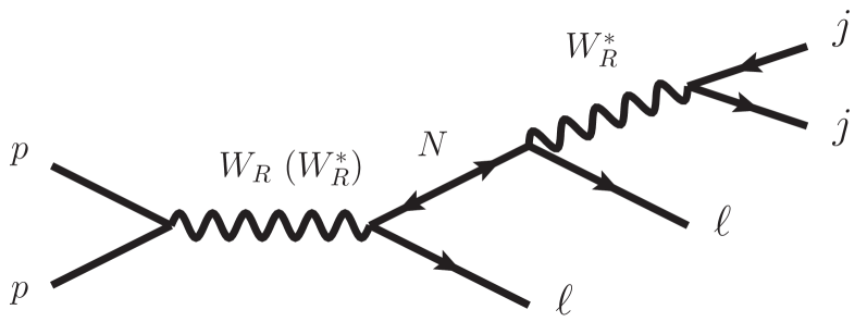
Figure 1: The Keung-Senjanović process. The final state leptons could be of same sign owing to the Majorana nature of $N$. The Drell-Yan production of $W_{R}$ and $N$ may be dominated by an off-shell $W_{R}^{*}$ exchange.

Pre-LHC studies of the KS process were performed by ATLAS Ferrari:2000sp and CMS Gninenko:2006br . Because the heavy neutrino lifetime $l_{N}$ depends on its mass, the KS process leads to substantially different signatures depending on $m_{N}$. A roadmap for different $m_{N}$ was performed in Nemevsek:2011hz , using the early LHC data, where transitions from prompt to displaced and invisible signals were sketched out.

The standard region is the usual golden channel with $l_{N}\lesssim 0.02\text{ mm}$ and two isolated leptons resulting in the $\ell\ell jj$ signature that was revisited in Ng:2015hba ; Ruiz:2017nip . For lighter $N$, it transitions into the merged region, where one lepton and two jets merge into a single neutrino (or lepton) jet Mitra:2016kov , the $\ell j_{N}$ signature. Eventually, the neutrino becomes long-lived and the jet vertex becomes displaced, $\ell j^{d}_{N}$; we call this the displaced region Helo:2013esa ; Izaguirre:2015pga ; Dib:2014iga . The displaced vertex may lie in the inner detector or even in the external parts like calorimeters or muon spectrometers. Finally, the invisible region covers the remaining case when $l_{N}\gtrsim 5\text{ m}$ decays outside of the detector. In this work we systematically analyze all four relevant regions and provide sensitivity estimates throughout the entire parameter space.

Existing experimental searches address the standard KS region ATLASKS ; CMSKS ; CMS:2017ilm , while searches for $W^{\prime}\to\ell\nu$ ATLASWpMissing ; CMSWpMissing apply to the invisible region. However, no active search has been devoted to the merged and displaced regions so far. The purpose of this work to provide an assessment of the sensitivity of LHC in these cases and realistically cover the entire $m_{N}$ range. We focus our search on $W_{R}$ masses beyond the limit of $\sim 3.5\,\text{TeV}$, already excluded by the $W_{R}\to jj$ search ATLASDijet , and RH neutrino masses that range from $m_{N}\sim\text{ few GeV}$, in the invisible region, to $m_{N}\leq M_{W_{R}}$ beyond which the process becomes kinematically suppressed.

The $m_{N}$ region below $\sim 20\text{ GeV}$ is relevant for phenomenology because of the connection between the KS process at the LHC and the new physics contributions to neutrinoless double beta decay, as studied in Mohapatra:1980yp ; Tello:2010am ; Nemevsek:2011aa . We will return to this interesting connection below.

The work is organized as follows. In the following section we review the kinematics and momentum scales involved in the KS process, for both on-shell and off-shell $W_{R}$ production, and describe the diverse resulting signatures. In section II we study both prompt and displaced regions by simulating the background and signal in order to assess the sensitivity. In section III we study the invisible region where we recast the available search in the lepton plus missing energy channel, and also provide the sensitivity at future colliders. Section IV contains conclusions and an outlook, and a few Appendices contain the analytical details as well as the detailed description of the binning method used to assess the statistical sensitivity.

I The Keung Senjanović process at LHC.

The minimal LRSM is based on the weak gauge group $\mathcal{G}_{LR}=SU(2)_{L}\otimes SU(2)_{R}\otimes U(1)_{B-L}$ and a symmetry between the left and right sectors with equal gauge couplings $g_{L}=g_{R}$. Correspondingly, quarks and leptons are arranged in LR symmetric representations, $q_{L,R}=(u,d)_{L,R}$ and $\ell_{L,R}=\left(\nu,e\right)_{L,R}$. The $SU(2)_{R}$ gauge symmetry is broken spontaneously at some high scale together with the discrete LR symmetry, and the new gauge bosons $W_{R}$, $Z_{R}$ acquire their masses at that scale. For our purposes it is enough to consider the scale as $M_{W_{R}}$, which, for $g_{L}\approx g_{R}$, is already limited to be larger than $\sim 3.5\,\text{TeV}$ by the di-jet searches ATLASDijet . This also ensures the smallness of the mixing between left and right gauge bosons, which plays no significant role in the rest of the paper.

We are focusing on the search for the $W_{R}$ gauge boson, which has the following charged-current interactions

$$\frac{g_{R}}{\sqrt{2}}\left[V^{q}_{R}\,\bar{u}_{R}{\not{W}}_{R}^{+}d_{R}+V^{\ell}_{R}\,\bar{N}\not{W}_{R}^{+}\ell_{R}\right]+{\rm h.c.}$$ (1)

where, suppressing flavour indices, $V^{q}_{R}$ is the RH analog of the Cabibbo-Kobayashi-Maskawa mixing matrix, and $V^{\ell}_{R}$ is the flavour mixing matrix of RH neutrinos $N\equiv\nu_{R}$. The RH quark mixing angles inside $V^{q}_{R}$ are predicted in the LRSM model to be equal or very near to the standard LH mixings Zhang:2007fn ; Maiezza:2010ic ; Maiezza:2014ala ; Senjanovic:2014pva . Potentially small deviations play no significant role at colliders and we use the standard CKM matrix for the quark sector.

With the KS process Keung:1983uu , the LRSM offers a golden search for the new interaction mediated by $W_{R}$ in the presence of $N$. Once $W_{R}$ is Drell-Yan produced, its decay generates an on-shell $N$ that further decays through another off-shell $W_{R}^{*}$ into two jets plus a lepton or anti-lepton with equal probability, owing to its Majorana nature (see Fig. 1). The whole process is kinematically favored in the region $M_{W_{R}}>m_{N}$.

In contrast to the quark sector, the leptonic mixing matrix $V^{\ell}_{R}$ is not predicted by the model. Instead, its entries can be probed directly at the LHC. The KS process allows to look for different leptonic flavours in the $\ell\ell jj$ signature Das:2012ii ; Vasquez:2014mxa . At the same time, also channels mediated by the Higgs $h$ or triplet Higgs $\Delta$ can be used to determine the heavy $N$ Majorana mass matrix. The Higgs option was dubbed the “Majorana Higgs” program, where channels such as $h\to NN$ Graesser:2007yj ; Maiezza:2015lza and $\Delta\to NN,h\to\Delta\Delta\to 4N$ Nemevsek:2016enw ; Dev:2016vle ; Dev:2017dui may be used to discover lepton number and flavour violation, and to measure the Majorana Yukawa couplings thereby discovering the spontaneous origin of $N$ masses.

Whichever is the source of information, measuring $V^{\ell}_{R}$ is essential to predict neutrino Dirac masses. Because of the LR parity that is built in the theory, an unambiguous connection between the Majorana and Dirac masses exists, which is transparent in the $\mathcal{C}$ Nemevsek:2012iq and slightly less so in the case of $\mathcal{P}$, see Senjanovic:2016vxw . The connection in turn predicts the Dirac couplings that can be observed at the LHC and low energies Nemevsek:2012iq .

The right-handed character of $W_{R}$ may be assessed by analyzing the final states angular correlations Ferrari:2000sp , as studied in Gopalakrishna:2010xm while invariant mass variables provide an additional handle for disambiguation Dev:2015kca . In addition, the extent of the Majorana nature character of $N$ can be characterized by same versus opposite sign of dileptons Das:2017hmg ; Gluza:2015goa .

Historically, searches Ferrari:2000sp ; Gninenko:2006br ; Nemevsek:2011hz ; ATLASKS ; CMSKS ; CMS:2017ilm focused on the on-shell production of $W_{R}$. The LHC however, especially in the designed high-luminosity phase, as well as future colliders, have the capability of probing higher masses for which the production may be dominantly off-shell (see for instance Ruiz:2017nip , where the analysis focuses on heavy to intermediate RH neutrino masses). Thus, in this section we review the features of the KS process in generality by describing the production of the prompt charged lepton and $N$ via an on- or off-shell $W_{R}$, making explicit the distribution of final states, which play a role in the LHC sensitivity.

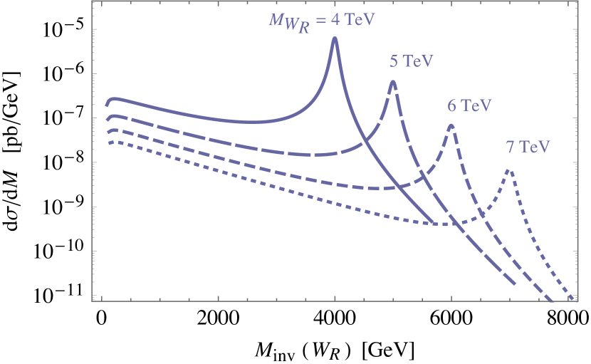
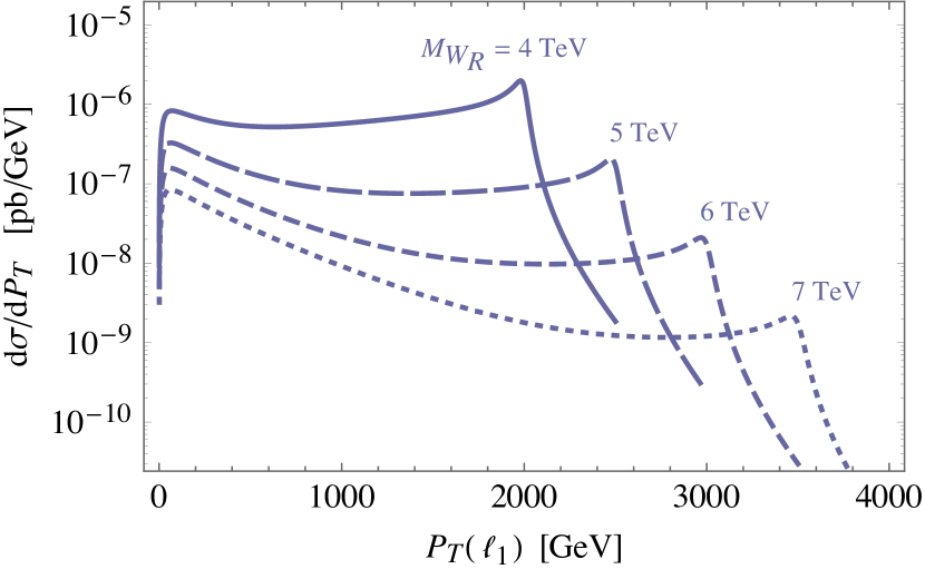
Figure 2: $W_{R}$ invariant mass distribution (upper) and primary lepton $p_{T}$ distribution (lower), for $M_{W_{R}}=4$–$7\,\text{TeV}$ (solid to dotted). For increasing $M_{W_{R}}$ the events on the on-shell $W_{R}$ peak become negligible, and the off-shell regime with a low invariant mass takes over. Similarly, the primary electron transverse momentum is peaked at low values on the lower plot.

On- and off-shell Drell-Yan production of $W_{R}$, $N$.
At the LHC the momentum available from parton constituents is enough to produce an on-shell $W_{R}$ until $M_{W_{R}}\lesssim 4\,\text{TeV}$, with the parton level cross section

$$\hat{\sigma}_{ij}^{W_{R}^{\pm}}(\hat{s})=\frac{\alpha_{2}\pi^{2}}{3}\left|V^{\text{\tiny CKM}}_{ij}\right|^{2}\delta\left(\hat{s}-M_{W_{R}}^{2}\right)\,.$$ (2)

For higher $W_{R}$ masses, the KS process takes place through an off-shell $W_{R}^{*}$. Assuming for simplicity a diagonal coupling of $W_{R}$ with a single generation lepton and RH neutrino, the parton level production cross section of $\ell N$ is

$$\hat{\sigma}_{ij}^{\ell N}(\hat{s})=\frac{\alpha_{2}^{2}\pi}{72\hat{s}^{2}}\left|V^{\text{\tiny CKM}}_{ij}\right|^{2}\frac{\left(\hat{s}-m_{N}^{2}\right)^{2}\left(2\hat{s}+m_{N}^{2}\right)}{\left(\hat{s}-M_{W_{R}}^{2}\right)^{2}+M_{W_{R}}^{2}\Gamma_{W_{R}}^{2}}$$ (3)

and we refer to Appendix B for details.

In the upper plot of Fig. 2 we show the distribution of $W_{R}$ invariant mass for the $\ell N$ production at LHC, which shows that the transition between the two regimes is gradual. The production clearly becomes dominated by the off-shell contribution when $M_{W_{R}}\gtrsim 5\,\text{TeV}$. One sees that the $s$-channel energy involved is always below $\sim\text{TeV}$, as the $W_{R}^{*}$ exchange becomes a contact interaction. A similar effect is seen in the momentum distribution of $N$ and that of the primary charged lepton $\ell_{1}$, which is progressively peaked at lower energies (lower plot in Fig. 2). This has implications for the boost inherited by the neutrino, and thus on its decay length to be analyzed below.

Taking kinematics and PDFs into account, the $pp\to W_{R}\to\ell N$ production cross section is shown in Fig. 3 as a function of the $W_{R}$ mass and for a selection of center of mass energies and $N$ masses $m_{N}=\left(50,100,500,1000,M_{W_{R}}/2\right)\text{ GeV}$ to cover both the light $N$ regime up to the standard KS regime.

While heavier $m_{N}$ are suppressed by phase space, for larger $M_{W_{R}}$ the off-shell process favors lighter $N$s that show a relative enhancement. Their production is still significant via $W_{R}^{*}$, as long as there is sufficient energy available from the parton distribution functions. This has implications for the signals analyzed below.

Indeed, one observes that the regime of light neutrino is particularly promising: already with an integrated luminosity of $100\text{ fb}^{-1}$, hadron colliders can probe $W_{R}$ up to scales comparable to the available center of mass energy. Keeping in mind the regime of light $N$, we review the kinematics of its decay at the parton level and as seen by the detector.

Figure 3: Drell-Yan production cross section of $pp\to W_{R}^{\pm}\to\ell^{\pm}N$. For each indicated interaction energy, the curves from upper to lower are relative to $m_{N}=50,100,500,1000,M_{W_{R}}/2$, showing normal phase space suppression. In addition, notice the relative enhancement of the lighter $m_{N}$ curves for heavier $W_{R}$, where the $\ell N$ is produced via off-shell intermediate $W_{R}$. The bands represent the uncertainty due to different PDF sets.

Neutrino width and displacement. The neutrino width is dominated by the decay into a lepton and a quark pair. Below the top mass, the width of $N$ is well approximated by

$$\frac{\alpha_{2}^{2}m_{N}^{5}}{64\pi M_{W_{R}}^{4}}\sum_{u,c;d,s}\left|V_{ud}^{\text{\tiny CKM}}\right|^{2}\simeq\frac{1}{2.5\,\text{mm}}\frac{(m_{N}/10\,\text{GeV})^{5}}{(M_{W_{R}}/3\,\text{TeV})^{4}}.$$ (4)

In Appendix A we discuss the exact width, valid also for heavier $m_{N}$.

For progressively lighter $N$ and heavier $W_{R}$, the lifetime becomes on the order of meters and in the regime of $m_{N}\sim 10\,\text{GeV}$ the ratio $\Gamma_{N}/m_{N}\sim 10^{-12}$ becomes tiny, leading to issues with event generation, as described in Section II.

The decay length in (4) is further increased by the boost from the $W_{R}$ decay. For instance, in case the $W_{R}$ is produced on shell and practically at rest, the boost is simply given by $M_{W_{R}}/2m_{N}$. On the other hand, for higher $M_{W_{R}}$ the $W_{R}^{*}$ is necessarily off-shell. Its invariant mass is small but it still transmits momentum to the primary lepton and to $N$ from the originating partons (see Fig. 2). For the LHC, these boost factors can be approximated by

$$\gamma_{N}\simeq\begin{cases}\frac{M_{W_{R}}}{2m_{N}},&W_{R}\to\text{on-shell},\\[4.30554pt] \frac{1\text{ TeV}}{m_{N}},&W_{R}\to\text{off-shell},\end{cases}$$ (5)

where the second estimate was performed by the Monte Carlo study. For e.g. $m_{N}=10\,\text{GeV}$ the boost factor changes from a maximum of $\sim 250$, to the asymptotic $\sim 100$. Fig. 4 reports such laboratory decay length including this transition.

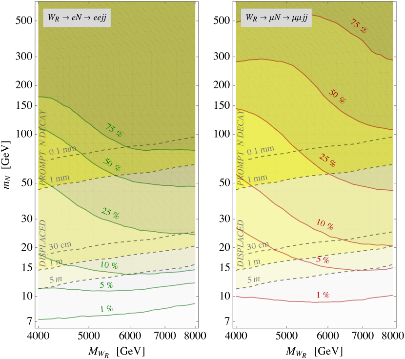
Figure 4: Left (right) plot: percentage of secondary leptons passing the isolation requirements is shown by the solid green(red) contours for the electron (muon) channel. Their average displacement from $N$ decay is shown in dashed black contours, and the yellow shaded regions mark the prompt or displaced $N$ decays showing that $\sim 25\%$ of electrons and $\%10$ of muons are isolated below 100 GeV. The lower white region corresponds to decays of $N$ outside of the inner tracker at $\gtrsim 30\text{ cm}$ or the entire detector $\gtrsim 5\text{ m}$.

Lepton isolation. For lower neutrino masses, the boost factor reduces the angular distance between the secondary lepton and the final jet(s) originating from $N$ decay. As soon as this angle goes below the isolation parameters required by the experimental detection, the lepton is not recognized and gets included in the jet instead. In Fig. 4 we display the percentage of surviving isolated leptons for the LHC at $\sqrt{s}=13\text{ TeV}$. We note that for $M_{W_{R}}\gtrsim 5\,\text{TeV}$, where $W_{R}$ is produced increasingly off-shell, the $N$ boost declines as in Eq. (5), such that secondary leptons are more easily isolated.

Already for $m_{N}<70\text{ GeV}$ where $N$ decays start to become visibly displaced, half or more of secondary leptons are not isolated anymore. The standard $\ell\ell jj$ case then turns into a single isolated lepton and another jet containing the secondary lepton, $\ell j$. The important conclusion here is that as $m_{N}$ is lowered, secondary leptons become non-isolated before being displaced. Thus the secondary lepton will be merged in a completely displaced merged neutrino jet.

In summary, in the light neutrino mass regime, the signature of the process consists typically of a single prompt lepton and another jet. While this final state does not offer the handle of LNV, it does show a characteristic displacement of the neutrino jet. Eventually for very low RH neutrino mass, the entire displaced jet is generated outside the detector and manifests as missing energy.

To analyze these different signatures, we separate the cases in four regions as outlined in the introduction:

1. The standard KS region, which for LHC requires $m_{N}\gtrsim$150–200 GeV, features two leptons and two jets ($\ell\ell jj$). The leptons are of same sign in half of the cases due to the Majorana nature of $N$, and the invariant masses $m_{\ell\ell jj}^{\text{inv}}$ and $m_{\ell jj}^{\text{inv}}$ can reconstruct the masses of $W_{R}$ and $N$.

2. The merged region where the signature is a prompt lepton and a jet containing the products of $N$ decay including the secondary lepton ($\ell j_{N}$). The small mass of $N$ makes it difficult to reconstruct its mass through the $j_{N}$ invariant mass. Still, $M_{W_{R}}$ can be identified via the invariant mass of $m_{\ell j_{N}}^{\text{inv}}$.

3. The displaced region where the merged neutrino jet appears at a visibly displaced distance from the primary vertex ($\ell j^{d}_{N}$).

4. The invisible region where the jet appears outside the detector and manifests itself as missing transverse momentum ($\ell\not{E}_{T}$).

The separation between the above regions is not sharp, a fraction of events leaks from one region to another and eventually results in overlapping exclusion regions.

II The standard, merged and displaced KS

In this section, we assess the reach of the LHC in the standard, merged and displaced regions defined above.

We first discuss the intricacies of event generation and the procedure for identifying the jet displacement at the detector level. We then describe the relevant backgrounds and finally adopt a dedicated statistical procedure for assessing the signal sensitivity, designed to deal with correlated kinematical variables.

Event Generation. Commonly used multi-purpose Monte Carlo event generators such as MadGraph are well suited to simulate the standard KS region. However, difficulties appear in dealing with extremely narrow resonances, as is the case in the merged, displaced and invisible regions where $\Gamma/M\simeq 10^{-12}$ or less. The difficulties are related to insufficient numeric precision as well as to phase space integration coverage (see thesis for a detailed discussion). To avoid these issues and generate a reliable signal, we developed a custom event generator, made available on lrsite and described in the Appendix C. It generates events at parton-level, including the case of the off-shell $W_{R}$ as well as light or heavy RH neutrino. The NLO corrections of $W_{R}$ production, are taken into account with a $K$-factor that is well approximated by a constant value of 1.3 (see Mitra:2016kov for a recent computation). Events are finally hadronized using Pythia 6.

The presence of an energetic primary lepton ensures triggering of the events, and leaves us with just the problem of identifying the possibly displaced jet.

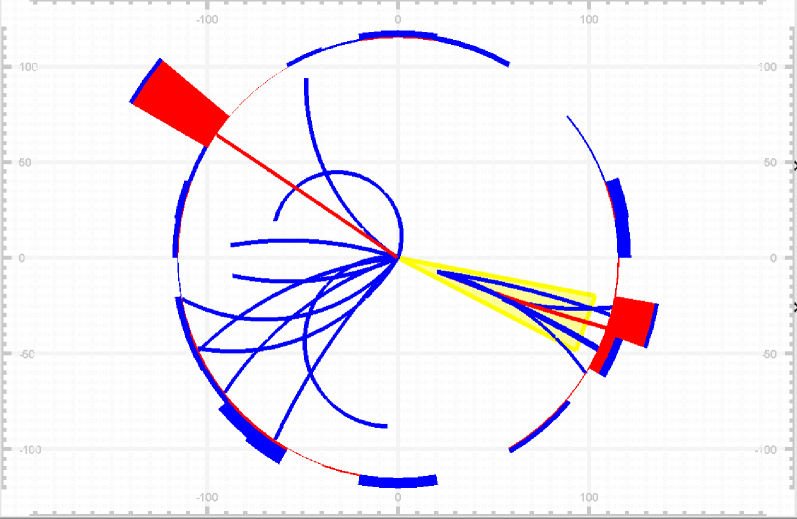
Figure 5: A typical event featuring the prompt electron and a merged jet on the opposite side, including the secondary electron and constituent tracks from a $\sim 3\,$cm-displaced vertex. Both electron tracks are drawn in red. (Picture produced using the Delphes deFavereau:2013fsa event viewer.)

Recognizing displaced jets. At detector level, we have adopted the Delphes software deFavereau:2013fsa , improved by developing a custom module for jet displacement recognition.

The problem of identifying the displacement of the jet origin is quite nontrivial for a number of reasons, mainly because inside of each jet a number of tracks with displaced origin are typically always present (due to decays of long-lived hadrons like e.g. $B$-mesons) and make part of the jet sub-structure. Moreover, a number of soft tracks are coming from the primary vertex processes that usually accompany any displaced hard process. These make it hard to detect its presence. A number of approaches to cope with these problems, i.e. to probe the jet-substructure have been devised that suit particular scenarios. The strategy that we adopt is as follows: jet displacement is defined as the minimum displacement among the tracks associated with the jet which have $p_{T}$ larger than some threshold, calibrated to $50\,\text{GeV}$. This simple but robust algorithm reproduces the correct displacement in 95% of the signal cases. In Fig. 5 we display a typical event where the displaced jet can be recognized by the displaced vertex from which its most energetic constituent tracks are originating.

It is worth mentioning that in defining each track displacement, also the smearing of the track vertex position due to (momentum dependent) detector resolution was implemented  vertexsmearing ). The minimal resolution is $\sim$0.01–0.02–0.1 mm, therefore below these values no displacement can in any case be appreciated. We do not apply extra suppression factors due to efficiency of displaced vertex recognition. In this regard, we note that at displacements between few millimeter and few centimeters, vertex efficiency is typically large $\sim 80\%$ Aaboud:2017iio , while a dedicated vertexing algorithm may need to be implemented to detect displacements below few millimeters. On the other hand, we discard jets with displacement beyond 30 cm, for which the vertex reconstruction by tracking appears largely unfeasible.

Finally, momentum resolution is also important especially for muons, because for one it gets progressively worse for large momentum $\sim\text{TeV}$, and because the secondary muon can become part of the jet, thus contributing to its invariant mass. As a benchmark, we assume the momentum resolution as studied in momentumresolution for the ATLAS detector.

  

  

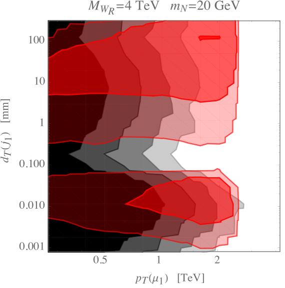
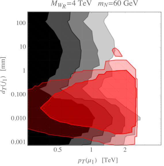
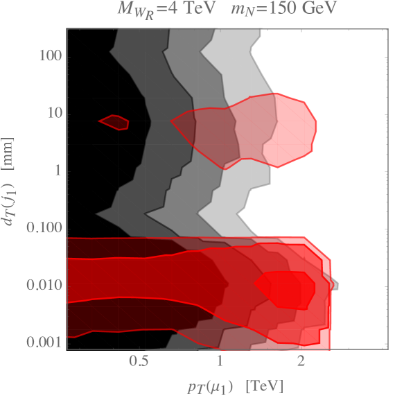
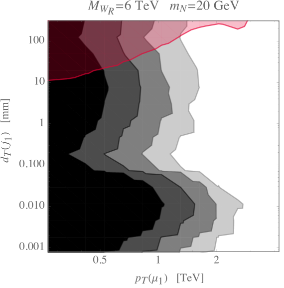
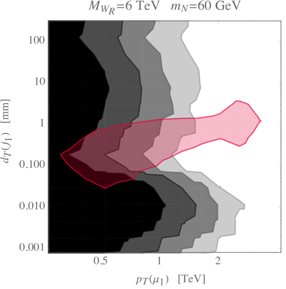
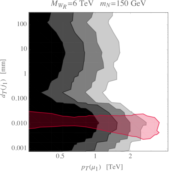
Figure 6: Event distribution in $p_{T}$ and displacement of the hardest jet. Shown are background (gray) and signal (red) for some sample values of $M_{W_{R}}=4,6\text{ TeV}$ (upper, lower) and $m_{N}=20,60,150\text{ GeV}$ (left to right). The distributions are exemplified with a binning grid of $15\times 15$, the increasingly dark shading referring to bins with respectively more than $0.1$, $1$, $10$, $100$ events.

Backgrounds. The dominant backgrounds contributing to this process are production of single or double vector bosons plus jets as well as production of $t\bar{t}$ plus jets.

While prohibitive to generate in full strength, we can take advantage of the fact that due to Eq. (5) the parton momenta in the signal are very rarely less than a few hundred GeV. Thus the background can be efficiently generated by imposing a cut of minimal $p_{T}>150\,\text{GeV}$ at parton level without loosing the signal. We use a stable version MadGraph 2.3.3, Pythia 6 and modified Delphes 3 with the anti-$k_{T}$ jet clustering algorithm with $\Delta R=0.3$. The number of background events simulated at generator level with the relative weights $\ll 1$, as well as the events recognized at detector level are:

background	# generator	weight	# detector
$V+012j$	22.46 M	0.021	9.93M
$VV+012j$	10.55 M	0.0028	4.61M
$t\bar{t}+012j$	10.47 M	0.024	4.38M

These are strongly reduced to respectively 378k, 15.6k, 65k expected detector level events when restricting the relevant kinematical variables to their loose range of interest (see below the first column of Table 1). A basic cut on $p_{T}(\ell)\gtrsim 1\,\text{TeV}$ could reduce them further to $\sim$ 250, 20, 7, or even less without sacrificing more than 20% of signal. Instead of adopting this rough procedure, we describe in the next paragraph a more efficient method of assessing the sensitivity.

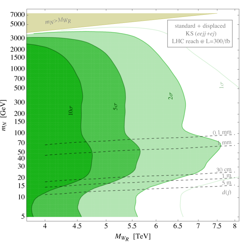
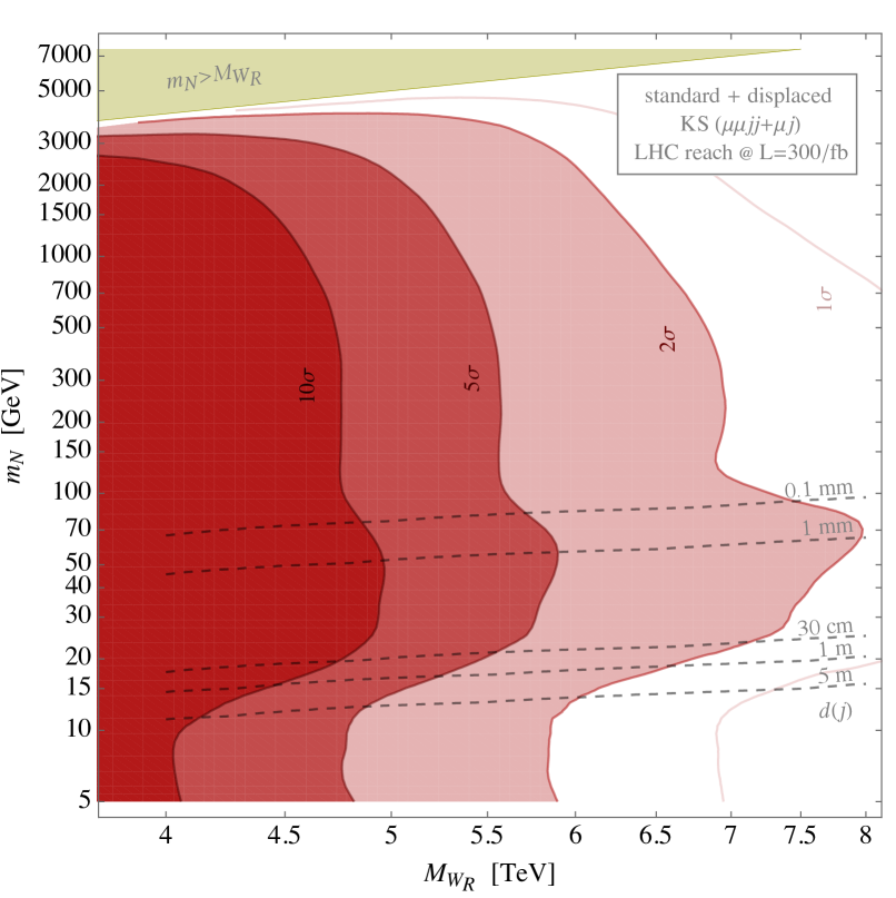
Figure 7: LHC sensitivity to the KS signal in the $M_{W_{R}}$ – $m_{N}$ plane, for integrated luminosity of $\mathcal{L}=300/$fb. Left, green (Right, red) frames show the sensitivity in the electron (muon) channel, obtained by combining the prompt $\ell\ell jj$ signature which features LNV as well as the displaced $\ell jj$ signature. Contours show the LHC reach at 1, 2, 5, 10 $\sigma$ C.L.

$\begin{array}[]{|lcc|rcccccccc|}\hline\cr~{}~{}~{}~{}~{}~{}\text{\color[rgb]{0.1,0.5,0.1} Electron Channel}\!\!\!\!\!\!\!\!\!\!\!\!\!\!\!\!&~{}~{}~{}~{}~{}~{}~{}~{}~{}~{}~{}~{}\mathcal{L}=300\,\mathrm{fb}^{-1}\!\!\!\!\!\!\!\!\!\!\!&&M_{W_{R}}\!:&4\,\text{TeV}&4\,\text{TeV}&4\,\text{TeV}&{}{}\hfil&6\,\text{TeV}&6\,\text{TeV}&6\,\text{TeV}&6\,\text{TeV}\\ \text{variable}&\text{range}&\text{\# bins}&m_{N}\!:&20\,\text{GeV}&300\,\text{GeV}&~{}2\,\text{TeV}{}&&20\,\text{GeV}&300\,\text{GeV}&~{}2\,\text{TeV}{}&~{}3\,\text{TeV}{}\\ \hline\cr p_{T}(\ell_{1})&\{150,4500\}\,\text{GeV}&{35}&&14.19&13.82&7.19&&1.03&1.77&1.22&0.80\\ d_{T}(j_{1})&\{0.001,300\}\,\text{mm}&{100}&&17.57&14.04&7.60&&2.02&1.91&1.38&0.97\\ \#(\text{jets})&1,2,3,4&{4}&&17.88&14.20&7.94&&2.24&2.04&1.47&1.08\\ \#(\text{leptons})&1,2&{2}&&17.97&14.90&9.08&&2.30&2.23&1.60&1.22\\ \#(\text{same sign})&0,1&{2}&&18.00&15.71&9.85&&2.32&2.61&1.70&1.30\\ m^{\text{inv}}_{\ell_{1}j_{1}}&\{200,8500\}\,\text{GeV}&{20}&&18.82&17.24&10.91&&2.81&3.03&1.91&1.47\\[2.15277pt] \hline\cr\end{array}$

Table 1: Grid binning variables and progressive sensitivities obtained with $300\,\text{fb}^{-1}$, for a selection of points in parameter space, representing the regimes of single lepton and displaced jet, single lepton and jet, and standard two leptons plus two jets.

Assessing the sensitivity. Examples of event distributions are reported in Fig. 6 in the plane of primary lepton momentum versus hardest jet displacement. We see that as the mass scales vary, the relative position of signal and background changes. In particular, because the jet displacement for the signal depends strongly on $m_{N}$, the signal region can overlap or instead be separated from one or more regions dominated by backgrounds. In situations like this, the effectiveness of the usual method of devising selection cuts is limited.

For this reason, instead of adapting the selection cuts to the values of model parameters, we prefer to devise a simpler and more robust method to assess the sensitivity. The method is a straightforward multi-bin generalization of the usual $s/\sqrt{s+b}$ measure relative to single bin Poisson-counting experiments. It combines single bin sensitivities of a multidimensional grid as the sum in quadrature, including the bins dominated by backgrounds,

$$\text{sensitivity}\ \Sigma=\left[\sum_{i\in\text{bins}}\frac{s_{i}^{2}}{s_{i}+b_{i}}\right]^{1/2}.$$ (6)

In Appendix D we describe in detail the formal aspects together with statistical and systematic uncertainties, also commenting on the binning dependence.

The binning grid that we adopt here spans the variables as described in the first column of Table 1, with broad enough intervals. In choosing the number of bins, we took care not to refine the binning below the resolution in the relevant kinematic variable(s). In the same table we also report the effectiveness of successive binning procedures in different kinematical variables for a selection of $(M_{W_{R}},m_{N})$. These are representative of the regime of lepton non-isolation with jet displacement, the standard KS regime with LNV, and also of on-shell versus off-shell $W_{R}$.

Finally, the maximal statistical and systematic uncertainty on the sensitivity can be quoted as $\pm 0.5$ and $\pm 0.01$, as discussed in Appendix D.

The result of the analysis is shown in Fig. 7 for both the muon and electron channel. Starting from below, i.e. from the most displaced region, we see that as soon as the displacement of neutrino decay can be detected by the tracker, i.e. below 30 cm, displacement helps in raising the sensitivity, which features a bump, for masses up to $m_{N}\sim 40$–$60\,\text{GeV}$. Thus, in this region, even if LNV is not observable, a very good sensitivity can be achieved by discriminating on the jet displacement. The result is a promising reach of more than 7 TeV, at 95% C.L..

Just above, in the prompt but merged region with $150\,\text{GeV}\lesssim m_{N}\lesssim\text{TeV}$, the sensitivity is lower due to phase space suppression. Nevertheless, as soon as genuine LNV becomes observable, the presence of same sign leptons acts as a complementary variable. In the standard KS regime where LNV helps, the combined effect leads to a plateau up to circa $m_{N}\sim\text{TeV}$ or 500 GeV, with sensitivity to circa $M_{W_{R}}\sim 6.5\,\text{TeV}$ at 95% C.L..

Above that, the KS process becomes increasingly suppressed by kinematics and sensitivity drops.

  

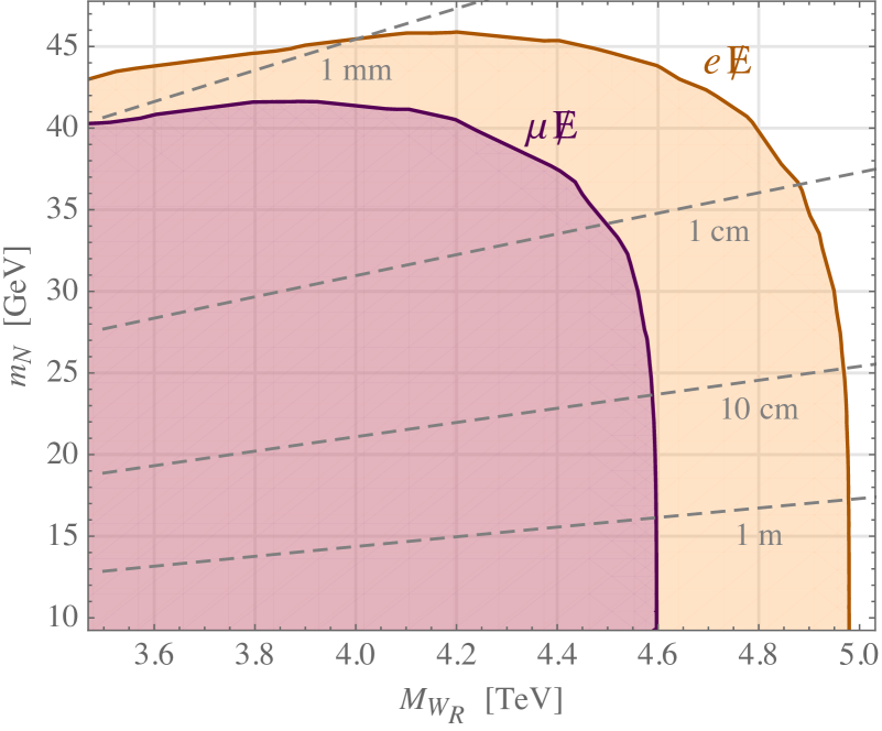
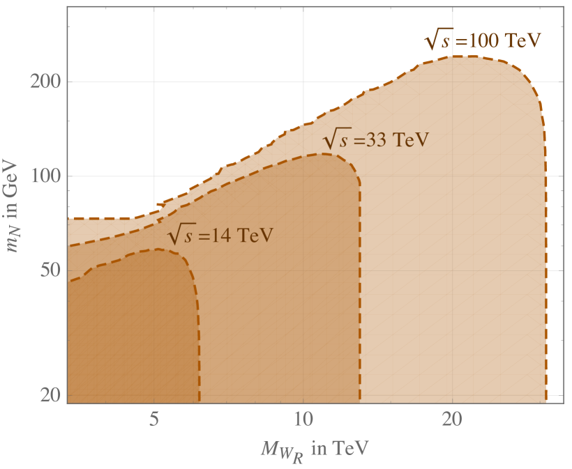
Figure 8: The $\ell+$missing energy channel. Left: exclusion region with present LHC data, recast from ATLASWpMissing ; the average boosted $N$ lifetime is also shown as dashed lines. The difference in electron and muon channels is due to the difference in measured events. Right: reach of this channel for 14, 33, 100 TeV center of mass energy; muon and electron channel basically coincide.

III The invisible KS

A separate assessment can be provided for the region where $N$ decays outside of the detector. In fact, in this region a very clean signature appears with a high-$p_{T}$ charged lepton and significant missing energy carried away by $N$. This happens for fairly light $m_{N}\lesssim 10\,\text{GeV}$, which may be motivated by having a warm DM candidate LR_WDM .

The simple $2\to 2$ kinematics of the process allows for a straightforward recast of the existing $W^{\prime}\to\ell\nu$ searches ATLASWpMissing ; CMSWpMissing , as well as sensitivity estimates for future colliders. To this end, it is useful to compute the distribution over $m_{T}=2p_{T}$ for signal events with $N$ decaying outside the detector radius, taken to be $l_{0}=5\,\text{m}$

$$\begin{split}\frac{\mathrm{d}\sigma}{\mathrm{d}m_{T}}=\alpha_{2}^{2}\frac{\pi}{24}p_{T}\int_{\tau_{-}}^{1}\int_{\frac{\tau_{-}}{x_{1}}}^{1}\mathrm{d}x_{1,2}\frac{\left(\hat{s}-m_{N}^{2}-2p_{T}^{2}\right)\pm 1}{\sqrt{\left(\hat{s}-m_{N}^{2}\right)^{2}-4p_{T}^{2}\hat{s}}}\\ \frac{e^{-l_{0}/L_{\pm}}\,\varepsilon^{\pm}_{\ell}(p_{T},\eta_{\ell})}{\left(\hat{s}-M^{2}\right)^{2}+\left(\Gamma M\right)^{2}}\left|V_{ud}V_{\ell N}\right|^{2}f_{u}(x_{1,2})f_{\overline{d}}(x_{2,1}),\end{split}$$ (7)

where $\tau_{-}=\frac{1}{s}\big{(}m_{N}^{2}+2p_{T}^{2}+2p_{T}\sqrt{m_{N}^{2}+p_{T}^{2}}\big{)}$ and $\hat{s}=x_{1}x_{2}s$. The sum goes over $u,d$ quarks, both lepton charges and the two $\hat{t}$ branches

$$\hat{t}_{\pm}=\frac{\hat{s}\left(\tau_{0}-1\right)}{2}\left(1\pm\sqrt{1-\frac{4p_{T}^{2}}{\hat{s}(\tau_{0}-1)^{2}}}\right),$$ (8)

with $\tau_{0}=m_{N}^{2}/\hat{s}$. The lab frame decay length

$$L=\frac{p_{T}}{m_{N}\,\Gamma_{N}}\sqrt{1+\left(1+\frac{m_{N}^{2}}{p_{T}^{2}}\right)\sinh(\eta_{N})^{2}},$$ (9)

is given by $p_{T}$ and $\exp(2\eta_{N})=-x_{1}/x_{2}\left(1+\hat{s}/\hat{t}\right)$. The $\varepsilon_{\ell}$ are experimentally determined charged lepton efficiency maps usually given in the $p_{T}-\eta_{\ell}$ plane, with $\exp(2\eta_{\ell})=-x_{2}/x_{1}\left(1+\hat{s}/(\hat{t}-m_{N}^{2})\right)$.

The main backgrounds to this process are the SM single $W$, top quark and multi-jet production. Integrating (7) in the entire $m_{T}\in[3-7]\,\text{TeV}$ bin and taking the corresponding background from ATLASWpMissing , the exclusion in the $M_{W_{R}}-m_{N}$ plane is obtained and shown on the left panel of Fig. 8 and reproduced below in the comprehensive Fig. 9.

Because of the exponential tail and the boost factor, the limit extends to a very small proper decay length of $N$ below 1 cm and thus covers the range of $m_{N}$ well in the $\mathcal{O}(10\,\text{GeV}$ range for the LHC, as seen in Fig. 8. Of course, in the $m_{N}\to 0$ case, the extremal limit in ATLASWpMissing is reproduced.

The limits in the electron and muon channels differ due to the difference in the observed data events, not so much due to the efficiencies or backgrounds. In addition to $e$ and $\mu$, the $\tau$ channel search was also performed by the CMS collaboration CMSWpMissing . However, because of lower luminosity used in the search as well as a slightly lower efficiency, the bound goes only up to 3.3 TeV and is not yet competitive with the di-jet limit.

Due to the cleanliness of the $\ell\not{E}$ final state, the process provides excellent sensitivity to $W_{R}$, going almost to the kinematical endpoint of $6.5\,\text{TeV}$ for the HL-LHC program with $\sqrt{s}=14\text{ TeV}$ and $3\text{ ab}^{-1}$, see Fig. 8. In order to estimate the sensitivity the background $m_{T}$ bins were rescaled to proper energies and the global sensitivity formula in Eq. (6) was used. Assuming the same collected luminosity, the future $\sqrt{s}=33(100)\,\text{TeV}$ $pp$ machines would cover the $W_{R}$ masses up to $M_{W_{R}}<13.5(33)\,\text{TeV}$ and $m_{N}\lesssim 120(250)\,\text{GeV}$, well in the $\mathcal{O}(100)\,\text{GeV}$ region, as seen on the right panel of Fig. 8.

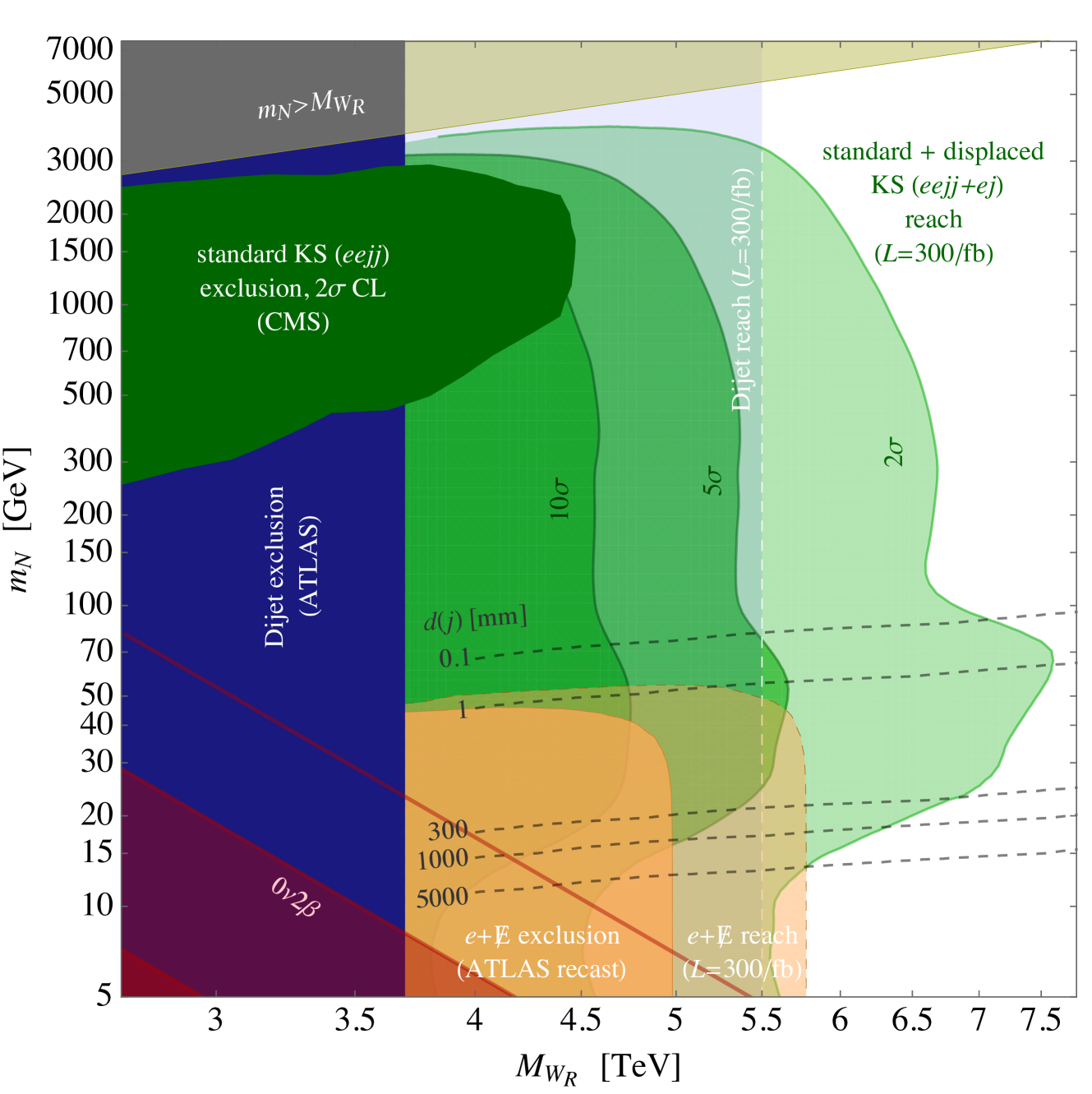
Figure 9: Summary plot collecting all searches involving the KS process at LHC, in the electron channel. The green shaded areas represent the LH sensitivity to the KS process at $300/$fb, according to the present work. The rightmost reaching contour represents the enhancement obtained by considering jet displacement.

IV Conclusions and roadmap

The case of a TeV-scale Left-Right symmetric extension of the Standard Model, which provides a complete theory of neutrino masses and an understanding of the origin of parity breaking, still resists as a viable case, notwithstanding the rapid progress of LHC in probing and excluding the scales of new physics. The main channel for discovering the RH gauge boson $W_{R}$ in connection with the RH neutrino $N$ is the so called Keung-Senjanović (KS) process Keung:1983uu , $pp\to W_{R}\to\ell N\to\ell\ell jj$. The constraints from direct searches CMSKS ; ATLASKS , from flavour changing processes Bertolini:2014sua ; Maiezza:2014ala and model perturbativity  Maiezza:2016bzp point to a scale of the new RH interaction which is now at the fringe of the LHC reach, so the residual kinematically accessible range will be probed in the next year of two.

In this work we reconsidered this process and addressed the regime of light $N$ ($m_{N}\lesssim 100\,\text{GeV}$) which leads Nemevsek:2011hz to long lived RH neutrino and thus to displaced vertices from its decay to a lepton and jets. This complements previous studies and gives a comprehensive overview of the collider reach covering the full parametric space.

To this aim, we classified the signatures resulting from the KS process, depending on the RH neutrino mass, in four regions: 1) a standard region where the final state is $\ell\ell jj$, with half of the cases featuring same-sign leptons, testifying the lepton number violation. 2) a merged region, with lighter and more boosted $N$, in which its decay products are typically merged in a single jet including the secondary lepton, resulting in a lepton and a so called neutrino jet $\ell j_{N}$. 3) a displaced region, for $m_{N}\sim 10-100\,\text{GeV}$, in which the merged jet $j_{N}$ is originated from the $N$ decay at some appreciable displacement from the primary vertex, typically from mm to 30 cm where the silicon tracking ends and detection of displaced tracks becomes unfeasible. 4) an invisible region, for $m_{N}\lesssim 40\,\text{GeV}$, in which $N$ can decay outside the tracking chambers of even the full detector, leading thus to a signature of a lepton plus missing energy, $\ell E\!\!\!\!/$.

We assessed the reach in all these regions by scanning the $m_{N}$, $M_{W_{R}}$ parameter space, up to $\mathcal{O}(10)\text{ TeV}$. For $W_{R}$ masses beyond $\sim 5\,\text{TeV}$ the process is dominated by the off-shell $W_{R}^{*}$ production, and we noted that, by this mechanism, for $m_{N}\lesssim 500\,\text{GeV}$ the final cross section gets an enhancement (see Fig. 3) due to the typical $W_{R}^{*}$ invariant mass $\sim\text{TeV}$ (see Fig. 2). This eases probing the light-$N$ region with respect to previous studies.

The results are summarized in the comprehensive Fig. 9. The analysis of the novel displaced region is offered for the first time in this work and shows that by using the decay displacement as a discriminating variable this region has a very promising highest potential of detection, reaching up to $M_{W_{R}}\simeq 7$–7.5 TeV.

In order to carry out the above analysis the following procedure was adopted. After noting that multipurpose event generators do not deal well with long lived particles, we developed a dedicated generator (see Appendix C and lrsite ). This was followed by standard Pythia hadronization and showering. Also detector simulation had to be updated by developing custom Delphes modules, in order to realistically detect the jet displacement (see section II). See thesis for additional details.

The basic signature of at least one energetic prompt lepton plus one possibly displaced jet ensures triggering and allowed us to estimate the relevant background of vector boson(s) plus jets, as described in section II.

The interplay between the primary lepton momentum, jet displacement and other variables calls for an ad hoc procedure for assessing the LHC sensitivity, whereas standard selection cuts would be cumbersome and ineffective. We devised a simple and robust statistical method which generalizes the $s/\sqrt{s+b}$ measure to binned distributions, and also cross checked it versus the more sophisticated method using Multi Variate neural networks. The results were broadly consistent but even better in sensitivity with respect to the neural network approach, which is also much slower.

In Fig. 9 we report the expected sensitivity in the electron channel as analyzed in this work, and collect all present constraints. These include the current KS search from CMS CMSKS and ATLAS ATLASKS and the $W_{R}\to jj$ ATLASDijet excluding up to $M_{W_{R}}\lesssim 3.7\,\text{TeV}$. A similar sensitivity on $Z_{LR}$ from dilepton bounds was reported in Lindner:2016lpp , while the $h,Z^{\prime}\to NN$ were studied in the context of a related $B-L$ model  Kang:2015uoc ; Accomando:2016rpc ; Accomando:2017qcs .

In the lower-left part of the plot, we add the region connected with $0\nu 2\beta$-decay, showing both the parameter space excluded by current probes  Agostini:2013mzu ; KamLAND-Zen:2016pfg as well as sensitivity of the next round of experiments. The relevant parameter space coincides by now with the lowest neutrino masses, i.e. with the invisible region.

The prospects for detection at LHC in the three standard, merged and displaced regions are put together as the green shaded areas for 2, 5, 10 $\sigma$ sensitivity. The upper part of this contour traces the standard KS case of the $\ell\ell jj$ signature, while in the lower part the displacement helps in raising the sensitivity.

In the intermediate merged region, for which $0.01<m_{N}/M_{W_{R}}<0.1$, i.e. $m_{N}\simeq 50$–$500\,\text{GeV}$ before the onset of displacement, we obtain a promising sensitivity to $M_{W_{R}}\simeq 6.5\,\text{TeV}$, at $2\sigma$ C.L.. This region was analyzed also by the first study Ferrari:2000sp , reporting a limiting sensitivity to $\sim 6\,\text{TeV}$, and also by the recent work Mitra:2016kov that reported a lower figure, circa 5.2 TeV. Having checked that the relevant simulated backgrounds are equivalent, we attribute the improvement to our new binning procedure replacing the usual kinematical cuts. This region is also sensitive to complementary searches at the LHeC electron-proton collider with a prompt jet and (possibly displaced) $ejj$ vertex Lindner:2016lxq .

With an orange area we report the analysis of the invisible region, obtained by recasting the current search for $W^{\prime}$ in the $\ell E\!\!\!\!/$ signature. It covers the region of $m_{N}\lesssim 40\,\text{GeV}$, and we can presently exclude up to $M_{W_{R}}<5\,\text{TeV}$. With $300/$fb of integrated luminosity LHC will be able to exclude up to circa 5.7 TeV.

The most prominent feature of our results is a sensible improvement of the sensitivity as soon as the jet displacement is effective as a discriminating variable, see Fig. 7 for both muon and electron channels. For displacements of the order of 10 mm, one can probe $M_{W_{R}}$ as large as $\sim 7(7.5)\,\text{TeV}$ in the electron(muon) channel. For displacements below few mm the sensitivity could be even larger, as shown by the bump in Fig. 9 but a realistic assessment of the vertexing capabilities should be carried out in the concrete detector environment.

While there are no existing experimental searches that directly address the displaced vertex region, a very recent study was performed in Cottin:2018kmq by recasting to an existing ATLAS search for displaced vertices and missing energy Aaboud:2017iio . The authors find the existing search has poor sensitivity, and propose a relaxed $N_{trk}$ and $m_{DV}$ requirements to significantly enhance the efficiency. The region of interest for that search is for $m_{N}$ below 40 GeV, where the invisible decay proves to be more competitive, see the lower part of Fig. 9. Nevertheless, an improvement in sensitivity and going below the fiducial 4 mm displacement to access higher $m_{N}$ seems promising.

From the above results one can conclude that if one extends the current searches by considering also displacement of jets, in a realistic range up to 30 cm, the LHC search for the KS process can reach a sensitivity up to 7–8 TeVat 95% C.L., for RH neutrino masses down to $\sim 20\,\text{GeV}$.

Further improvements in the recognition of even more displaced jets, like so called emerging jets, or displaced muons as distant as the muon chambers are also subject of current study emerging , and they could extend the sensitivities to even lower RH neutrino masses.

V Acknowledgments

The work of MN was supported by the Slovenian Research Agency under the research core funding No. P1-0035 and in part by the research grant J1-8137. FN and GP are partially supported by the H2020 CSA Twinning project No. 692194 “RBI-T-WINNING” and by the Croatian Science Foundation (HRZZ) project PhySMaB.

Appendix A Width of $N$

Computing the three-body decay width becomes involved when masses of decay products have to be taken into account. In the case of $N$ decaying into a lepton and a quark pair, further complications arise in the squared amplitude when mass of $N$ becomes comparable with mass of $W_{R}$, since the invariant mass of the quark pair cannot be neglected.

However, the width can be computed numerically. Full squared amplitude, although lengthy, is straightforward to calculate (using FORM, for instance) and phase space can be split into two pieces: two-body decay of $N$ into lepton and $W_{R}$, and decay of $W_{R}$ into a quark pair. This introduces a nontrivial integral over invariant mass $q^{2}$ of a quark pair and over the solid angle $\mathrm{d}\Omega^{*}$ of one of the quarks in the rest frame of $W_{R}$. After boosting the quarks into the rest frame of $N$, the integral over $\mathrm{d}\Omega$ is simple, since the squared amplitude is a polynomial in $\cos\theta$. The width of $N$ for decaying into a lepton of mass $m_{l}$ and quark pair with masses $m_{1}$ and $m_{2}$ is then

$$\begin{split}\frac{\mathrm{d}\Gamma}{\mathrm{d}q^{2}}&=\frac{\alpha_{2}^{2}N_{c}}{128\pi}\frac{1}{m_{N}\left(q^{2}-M_{W_{R}}^{2}\right)^{2}}\\ &\times\lambda^{\frac{1}{2}}\left(\frac{m_{l}^{2}}{m_{N}^{2}},\frac{q^{2}}{m_{N}^{2}}\right)\lambda^{\frac{1}{2}}\left(\frac{m_{1}^{2}}{q^{2}},\frac{m_{2}^{2}}{q^{2}}\right)\mathcal{A}(q^{2}),\end{split}$$ (10)

where $\mathcal{A}(q^{2})$ is the spin-averaged amplitude with angular dependency integrated out (coupling constants and scalar part of $W_{R}$ propagator are pulled out) and $\lambda(x,y)=1+x^{2}+y^{2}-2x-2y-2xy$. The remaining integral over $q^{2}$, $(m_{1}+m_{2})^{2}\leq q^{2}\leq(m_{N}-m_{l})^{2}$, can be easily evaluated numerically to a very high precision.

Appendix B $N$ production with off-shell $W_{R}$

We collect here the cross section of the KS process via on- and off-shell $W_{R}$. For ease of notation the mass and width of $W_{R}$ are denoted in this section as $M$ and $\Gamma$.

On-shell $W_{R}$ production.

$$\hat{\sigma}_{ij}(\hat{s})=\frac{\alpha_{2}\pi^{2}}{3}\left|V^{\text{\tiny CKM}}_{ij}\right|^{2}\delta\left(\hat{s}-M^{2}\right),$$ (11)

$$\sigma=\frac{\alpha_{2}\pi^{2}}{3s}\sum_{\begin{subarray}{c}i=u,c\\ j=\bar{d},\bar{s}\end{subarray}}\left|V^{\text{\tiny CKM}}_{ij}\right|^{2}\int\limits_{\frac{M^{2}}{s}}^{1}\frac{\mathrm{d}x}{x}\,f_{ij}\left(x,\frac{M^{2}}{xs},M^{2}\right).$$ (12)

$N$ production cross section. The rate for the process

$$u_{i}(k_{1})+\bar{d}_{j}(k_{2})\to W_{R}^{+}\to l^{+}(p_{1})+N(p_{2}),$$ (13)

where $u_{i}$ is up-type quark and $\bar{d}_{j}$ is down-type antiquark, at the parton level is

$$\frac{\mathrm{d}\hat{\sigma}_{ij}}{\mathrm{d}\hat{t}}=\frac{\alpha_{2}^{2}\pi}{12\hat{s}^{2}}\left|V^{\text{\tiny CKM}}_{ij}\right|^{2}\frac{\hat{t}(\hat{t}-m_{N}^{2})}{(\hat{s}-M^{2})^{2}+M^{2}\Gamma^{2}}.$$ (14)

In the parton CMS frame, $\hat{s}=(\hat{k}_{1}+\hat{k}_{2})^{2}$, and

$$\hat{t}=(\hat{k}_{1}-\hat{p}_{1})^{2}=-\frac{\hat{s}-m_{N}^{2}}{2}\left(1-\cos\theta\right),$$ (15)

where $\theta$ is the angle between $\hat{\mathbf{k}}_{1}$ and $\hat{\mathbf{p}}_{1}$. The total parton-level cross section is then

$$\hat{\sigma}_{ij}(\hat{s})=\frac{\alpha_{2}^{2}\pi}{72\hat{s}^{2}}\left|V^{\text{\tiny CKM}}_{ij}\right|^{2}\frac{(\hat{s}-m_{N}^{2})^{2}\left(2\hat{s}+m_{N}^{2}\right)}{(\hat{s}-M^{2})^{2}+M^{2}\Gamma^{2}}.$$ (16)

To obtain inclusive rates, convolution with parton distribution is needed,

$$\sigma =\int\limits_{\frac{m_{N}^{2}}{s}}^{1}\frac{\mathrm{d}x_{1}}{x_{1}}\int\limits_{m_{N}^{2}}^{x_{1}s}\frac{\mathrm{d}\hat{s}}{s}\,\sum_{\begin{subarray}{c}i=u,c\\ j=\bar{d},\bar{s}\end{subarray}}\hat{\sigma}_{ij}(\hat{s})\,f_{ij}\left(x_{1},\frac{\hat{s}}{x_{1}s};Q^{2}\right),$$ (17)

where $\sqrt{s}$ is the center of momentum energy in laboratory frame,

$$\begin{split}f_{ij}(x_{1},x_{2};Q^{2})&=f_{i/p}(x_{1};Q^{2})f_{j/p}(x_{2};Q^{2})\\ &+f_{i/p}(x_{2};Q^{2})f_{j/p}(x_{1};Q^{2}),\end{split}$$

where $f_{i,j/p}(x;Q^{2})$ are parton distribution functions evaluated at momentum fraction $x$ and factorization scale $Q^{2}=\hat{s}$ (default in MadGraph for KS process). Difference between production of $W_{R}^{+}$ and $W_{R}^{-}$ is only in the parton distributions.

Relevant (kinematical) distributions can easily be derived from (14) and (16) by inserting the appropriate $\delta$-functions, for instance

$$\frac{\mathrm{d}\hat{\sigma}}{\mathrm{d}y}=\int\frac{\mathrm{d}\hat{\sigma}}{\mathrm{d}\hat{t}}\,\delta\left(y-g(\hat{t})\right)\,\mathrm{d}\hat{t}.$$ (18)

$W_{R}$ invariant mass distribution. Invariant mass distribution for $W_{R}$ is simply

$$\frac{\mathrm{d}\hat{\sigma}_{ij}}{\mathrm{d}M^{2}}=\hat{\sigma}_{ij}(\hat{s})\,\delta(M^{2}-\hat{s})$$ (19)

and then

$$\frac{\mathrm{d}\sigma}{\mathrm{d}M^{2}} =\sum_{\begin{subarray}{c}i=u,c\\ j=\bar{d},\bar{s}\end{subarray}}\hat{\sigma}_{ij}(M^{2})\int\limits_{\frac{M^{2}}{s}}^{1}\frac{\mathrm{d}x_{1}}{x_{1}s}\,f_{ij}(x_{1},\frac{M^{2}}{x_{1}s};Q^{2}).$$ (20)

Prompt lepton $p_{{}_{T}}$ distribution. Transverse momentum distribution for the prompt lepton is obtained by inserting

$$1=\int\limits_{0}^{|\mathbf{p}_{1}|}\mathrm{d}p_{{}_{T}}\delta(p_{{}_{T}}-|\mathbf{p}_{1}|\sin\theta)$$ (21)

into (14) and integrating over $\hat{t}$,

$$\begin{split}\frac{\mathrm{d}\hat{\sigma}_{ij}}{\mathrm{d}p_{{}_{T}}}&=\frac{\alpha_{2}^{2}\pi}{6}\left|V^{\text{\tiny CKM}}_{ij}\right|^{2}\frac{p_{{}_{T}}}{\sqrt{(\hat{s}-m_{N}^{2})^{2}-4\hat{s}p_{{}_{T}}^{2}}}\\ &\times\frac{\hat{s}-2p_{{}_{T}}^{2}-m_{N}^{2}}{(\hat{s}-M^{2})^{2}+M^{2}\Gamma^{2}}.\end{split}$$ (22)

The convolution with parton distributions gives then

$$\begin{split}\frac{\mathrm{d}\sigma}{\mathrm{d}p_{{}_{T}}}&=\int\limits_{\frac{\varepsilon_{T}^{2}}{s}}^{1}\frac{\mathrm{d}x_{1}}{x_{1}}\int\limits_{\varepsilon_{T}^{2}}^{x_{1}s}\frac{\mathrm{d}\hat{s}}{s}\,\sum_{\begin{subarray}{c}i=u,c\\ j=\bar{d},\bar{s}\end{subarray}}\frac{\mathrm{d}\hat{\sigma}_{ij}}{\mathrm{d}p_{{}_{T}}}f_{ij}(x_{1},\frac{\varepsilon_{{}_{T}}^{2}}{x_{1}s};Q^{2}),\end{split}$$ (23)

where $\varepsilon_{{}_{T}}=p_{{}_{T}}+\sqrt{p_{{}_{T}}^{2}+m_{N}^{2}}$.

Appendix C Generation of events for small $N$ width

The cross section for the full KS process

$$q_{i}(k_{1})\bar{q}_{j}(k_{2})\to l^{\pm}(p_{1})l^{\pm}(p_{2})j(p_{3})j(p_{4})$$ (24)

can be written as

$$\sigma=\int\mathrm{d}x_{1}\mathrm{d}x_{2}\sum_{u,d,h}\hat{\sigma}_{ud,h}(x_{1},x_{2})f_{ud}(x_{1},x_{2},Q^{2}),$$ (25)

where $\hat{\sigma}_{ud,h}$ is the partonic cross section with quark flavors $u$ and $d$ and helicity configuration denoted by $h$. The phase space in $\hat{\sigma}_{ud,h}$ can easily be split into a sequence of 2-particle ones, for example

$$\begin{split}\mathrm{d}\Phi(k_{1}+k_{2}\to\textstyle\sum_{1}^{4}p_{i})=\mathrm{d}\Phi(k_{1}+k_{2}\to p_{1}+q_{234})\\ \mathrm{d}\Phi(q_{234}\to p_{2}+q_{34})\mathrm{d}\Phi(q_{34}\to p_{3}+p_{4})\frac{\mathrm{d}q_{234}^{2}\mathrm{d}q_{34}^{2}}{(2\pi)^{2}},\end{split}$$ (26)

and each of them is simply

$$\mathrm{d}\Phi(P\to p_{1}+p_{2})=\frac{1}{8\pi}\lambda^{\frac{1}{2}}\left(\frac{p_{1}^{2}}{P^{2}},\frac{p_{2}^{2}}{P^{2}}\right)\frac{\mathrm{d}\Omega}{4\pi},$$ (27)

where $\mathrm{d}\Omega=\mathrm{d}\phi\,\mathrm{d}\!\cos\theta$ is the solid angle of $\mathbf{p}_{1}$ or $\mathbf{p}_{2}$ in the rest frame of $P$ with respect to some axis, most conveniently taken in the direction of $\mathbf{P}$. In order to generate the events, angles and invariant masses in (26), as well as parton momentum fractions, $x_{1}$ and $x_{2}$ are randomly sampled. Eq. (26) corresponds to one possible phase space mapping, given by the kinematical structure of a diagram(s) describing the process.

Difficulties in Monte Carlo event generation of the KS process arise from the sharp (and dominant) peak in the invariant amplitude coming from a very small width in the neutrino propagator. Adaptive integration methods may not be able to handle such extreme cases, however this problem can be easily solved by sampling the appropriate phase space variables according to the Breit-Wigner distribution (importance sampling).

Since KS process consists of multiple subprocesses (helicity combinations, ingoing and outgoing quarks) each with one diagram for opposite sign leptons or two diagrams for same sign leptons in the final state, events are generated using the multichannel method. Each channel corresponds to a specific subprocess and phase space mapping for different diagrams and carries a weight $\alpha_{i}$ and a probability density $g_{i}(\mathbf{x})$, such that $g(\mathbf{x})=\sum_{i}\alpha_{i}g_{i}(\mathbf{x})$ and $\sum_{i}\alpha_{i}=1$, where $\mathbf{x}$ are phase space variables. Weights $\alpha_{i}$ are thus probabilities of selecting different channels and can be optimized during event generation fo better performance weight_optim . A suitable way to optimize $\alpha_{i}$ was proposed in madevent , by introducing a basis of functions

$$f(\mathbf{x})=\sum_{i}f_{i}(\mathbf{x}),\quad f_{i}(\mathbf{x})=\frac{\left|\mathcal{M}_{i}\right|^{2}}{\sum_{j}\left|\mathcal{M}_{j}\right|^{2}}\left|\mathcal{M}_{\text{tot}}\right|^{2},$$ (28)

where $\mathcal{M}_{\text{tot}}=\sum_{i}\mathcal{M}_{i}$. The integral is now the sum of contributions with different peaking structures (contained in the amplitudes $\mathcal{M}_{i}$),

$$I=\int\mathrm{d}\mathbf{x}\,f(\mathbf{x})=\sum_{i}\int\mathrm{d}\mathbf{x}\,g_{i}(\mathbf{x})\frac{f_{i}(\mathbf{x})}{g_{i}(\mathbf{x})}=\sum_{i}I_{i},$$ (29)

and optimized weights are $\alpha_{i}=I_{i}/I$. This approach avoids the evaluation of all $g_{i}(\mathbf{x})$ for every point in phase space and the complications related to the correlations between $\alpha_{i}$ when the number of channels is large.

For the event generation software, as well as custom detector simulation and analysis, visit te web site lrsite .

Appendix D Assessing sensitivity

It is a common problem, prior to having experimental data available, to assess the sensitivity of an experiment to a given hypothesis of new physics, defined as the number of signal ($s$) events expected on top of a number of background ($b$) events. These may be single numbers as in a simple counting experiment, or binned distributions in relevant kinematical variables like in the present case.

In a (Poisson) counting experiment, equivalent to the case of a single bin, it is customary to define the sensitivity as $s/\sqrt{s+b}$. This can be understood as a measure of the “separation” between the expected distributions in the hypotheses of background-only and background plus signal (see below).

In the case of more bins distributed in one or more kinematical variables, the usual procedure is to define cuts that exclude regions in which backgrounds dominate, and finally assess the surviving number of signal and background events ($S_{tot}$, $B_{tot}$). The choice of cuts must be optimized in order to maximize the global sensitivity e.g. $S_{tot}/\sqrt{S_{tot}+B_{tot}}$. This procedure can become quite complex with an increasing number of variables and if the region that one would like to cut has a nontrivial shape in their multidimensional space. Sometimes the procedure of cutting away the high-background low-sensitivity bins is even impossible.

Consequently, one can ask whether one could just define a measure that automatically weighs the various bins according to their contribution to the sensitivity. The answer is simple and amounts to adding in quadrature the sensitivities associated to each bin, such that the global sensitivity is defined as (6)

$$\text{sensitivity}\ \Sigma=\left[\sum_{i\in\text{bins}}\frac{s_{i}^{2}}{s_{i}+b_{i}}\right]^{1/2},$$ (30)

where $s_{i}$, $b_{i}$ are the expected number of signal and background events in each bin and we stress that the sum runs on the full grid of bins in the multidimensional space of kinematical variables. The resulting method is able to assess the global sensitivity of the experiment in a straightforward manner without having to impose cuts.

We discuss here first the formal justification, then the statistical uncertainty on this measure, as well as the systematics due to different binning.

For a Poisson counting experiment with expected number of events $\mu s+b$, the likelihood function is

$$L(\mu)=\frac{(\mu s+b)^{n}}{n!}e^{-(\mu s+b)},$$ (31)

where $s$ ($b$) is the number of signal (background) events and $\mu$ is the signal rate parameter, i.e. $\mu=0$ corresponds to the background only hypothesis, while $\mu=1$ to the signal plus background hypothesis. The maximum likelihood estimator of $\mu$ is $\hat{\mu}=(n-b)/s$ and has clearly expectation $E[\hat{\mu}]=\mu$, while its variance is

$$V[\hat{\mu}]=E[\hat{\mu}^{2}]-E[\hat{\mu}]^{2}=\frac{\mu s+b}{s^{2}}\,.$$ (32)

At $\mu=1$ (signal hypothesis) the standard deviation of the estimator $\hat{\mu}$ is $\sigma_{\hat{\mu}}=\sqrt{s+b}/s$ and thus $s/\sqrt{s+b}$ can be interpreted as the expected significance with which one could reject $s$ if the signal is absent statrpp .

One can proceed similarly in the case of more bins, but it is useful to first rescale $\mu$ into $\nu=\mu\,s/\sqrt{s+b}$ such that the likelihood is

$$L(\nu)=\frac{(\nu\sqrt{s+b}+b)^{n}}{n!}e^{-(\nu\sqrt{s+b}+b)}$$ (33)

and the estimator is $\hat{\nu}=(n-b)/\sqrt{s+b}$. This has clearly expectation $\nu=s\mu/\sqrt{s+b}$ and variance $(\nu\sqrt{s+b}+b)/(s+b)$. In the hypothesis of signal, expectation is $s/\sqrt{s+b}$ and variance is 1.

Now we consider together all (uncorrelated) bins. In the case of signal the distribution of the vector $\{\hat{\nu}_{i}\}$ is centered at position $\{s_{i}/\sqrt{s_{i}+b_{i}}\}$, still with unit variance 1 in each dimension. So, the distribution of $\{\hat{\nu}_{i}\}$ in the case of signal is peaked there, inside a “hypersphere” of radius 1. On the other hand, the case of no signal is represented by the origin, $\{\hat{\nu}_{i}=0\}$.

Thus, the definition of sensitivity in (6) represents the distance of the origin from the center of the unit hypersphere, and it can indeed be taken as a measure of the significance with which one can exclude the signal in case of no signal. The sum in quadrature in (30) takes contributions from the bins where significance is high, and negligible increase from the bins with no signal or dominant background, as it has to be.

Uncertainty in sensitivity. Let us briefly discuss the statistical and systematic uncertainties which affect the sensitivity measure (6).

We can discuss the statistical uncertainty, if the distribution in bins remains smooth as binning is refined, i.e. if locally $s$, $b\sim 1/N_{bins}$. In this case, for each bin the uncertainty on its contribution to the sensitivity, $s_{i}^{2}/(s_{i}+b_{i})$, is $[s_{i}^{3}(4b_{i}+s_{i})/(s_{i}+b_{i})^{3}]^{1/2}$, such that the uncertainty on $\Sigma$ is obtained by summing in quadrature all bins and is

$$\sigma_{stat}\left(\Sigma\right)=\frac{1}{2\Sigma}\left[\sum_{i}\frac{s_{i}^{3}\left(4b_{i}+s_{i}\right)}{(s_{i}+b_{i})^{3}}\right]^{\frac{1}{2}}$$ (34)

Notice that all terms in the sums in (6) and (34) scale as $\sim 1/N_{bins}$, so the final statistical uncertainty is not increased with finer binning.

More interesting is the systematic error that can arise when, in refining the binning, one hits the limit of smoothness of the distribution. Typically this happens first for the background, that may be simulated with less statistics, due to the higher required computing time. One can ask what happens in case in some region of parameter space this overbinning leads to a background events concentrated in isolated bins, while the signal is still smooth. In this case, the contribution to the sum (6) will contain an increasingly larger number of bins with just signal, increasing the sensitivity, plus a fixed number of bins with background. As a limiting example, let us describe the case in which in a region with total events $S$ and $B$, all background is concentrated in a single isolated bin, while the signal still scales as $1/N_{bins}$. For simplicity we assume also that in this region the signal distribution is constant, $s_{i}=S/N_{bin}$. In the limit of very fine binning the isolated background bin disappears from the final result of the sensitivity:

$$\Sigma_{1}=\left[A+S\right]^{1/2},$$ (35)

where $A$ represent the contribution of the rest of the bin. This should be compared with the standard smooth background case:

$$\Sigma=\left[A+\frac{S^{2}}{S+B}\right]^{\frac{1}{2}}.$$ (36)

The difference between these two is an estimate of the systematic error induced by overbinning the background, and it can be approximated as (for non negligible $\Sigma$):

$$\sigma_{syst}\left(\Sigma\right)\simeq\frac{1}{2\Sigma}\frac{BS}{B+S}\simeq\frac{1}{2\Sigma}\min(B,S)\,.$$ (37)

From this result one finds that the systematic error can be quite small even with large $B$: indeed, if $S$ is small in the regions where there is isolated background $B$, there is small contribution to the sensitivity and also to the uncertainty.

Similar to what is done in the MVA analysis (see e.g. MVA ) the optimal approach would be to estimate the magnitude of $S$ by exploring a region around isolated backgrounds, in order to check whether an increased contribution to the uncertainty is indeed present or not, and wether a more coarse grained binning would be needed. To delimit the regions where the background has isolated bins is however a typically hard task, and thus it is difficult to asses the relevant $S$. Fortunately, from (37) we note that it is actually sufficient to limit the value of $B$, i.e. of the total number of background events that remain in isolated bins. In this way one can control the systematic uncertainty, albeit overestimating it. The consequent upper limit is the figure of merit which we quote in the table in the text,

$$\sigma_{syst}\left(\Sigma\right)<B_{isolated}/{2\Sigma}\,,$$ (38)

in order to make sure that overbinning of background has negligible impact on our results.

References

- (1) J.C. Pati, A. Salam, Phys. Rev. D 10 (1974) 275; R.M. Mohapatra, J.C. Pati, Phys. Rev. D 11 (1975) 2558;
- (2) G. Senjanović and R. N. Mohapatra, Phys. Rev. D 12 (1975) 1502. G. Senjanović, Nucl. Phys. B 153 (1979) 334.
- (3) P. Minkowski, Phys. Lett. B 67 (1977) 421; R.N. Mohapatra, G. Senjanović, Phys. Rev. Lett. 44 (1980) 912.
- (4) T. Yanagida, Workshop on unified theories and baryon number in the universe, ed. A. Sawada, A. Sugamoto (KEK, Tsukuba, 1979); S. Glashow, Quarks and leptons, Cargèse 1979, ed. M. Lévy (Plenum, NY, 1980); M. Gell-Mann et al., P. Ramond, R. Slansky, Supergravity Stony Brook workshop, New York, 1979, ed. P. Van Niewenhuizen, D. Freeman (North Holland, Amsterdam, 1980).
- (5) G. Beall, M. Bander and A. Soni, Phys. Rev. Lett. 48 (1982) 848.
- (6) R.N. Mohapatra, G. Senjanović and M.D. Tran, Phys. Rev. D 28 (1983) 546; K. Kiers, J. Kolb, J. Lee, A. Soni and G.-H. Wu, Phys. Rev. D 66 (2002) 095002 [hep-ph/0205082].
- (7) G. Ecker and W. Grimus, Nucl. Phys. B 258, 328 (1985).
- (8) Y. Zhang, H. An, X. Ji and R.N. Mohapatra, Phys. Rev. D 76 (2007) 091301 [arXiv:0704.1662 [hep-ph]] and Nucl. Phys. B 802 (2008) 247 [arXiv:0712.4218 [hep-ph]].
- (9) A. Maiezza, M. Nemevšek, F. Nesti and G. Senjanović, Phys. Rev. D 82, 055022 (2010) [arXiv:1005.5160 [hep-ph]].
- (10) S. Bertolini, J.O. Eeg, A. Maiezza and F. Nesti, Phys. Rev. D 86 (2012) 095013 [arXiv:1206.0668 [hep-ph]]; S. Bertolini, A. Maiezza and F. Nesti, Phys. Rev. D 88 (2013) 3, 034014 [arXiv:1305.5739 [hep-ph]].
- (11) S. Bertolini, A. Maiezza and F. Nesti, Phys. Rev. D 89 (2014) 9, 095028 [arXiv:1403.7112 [hep-ph]].
- (12) A. Maiezza, M. Nemevšek and F. Nesti, Phys. Rev. D 94 (2016) no.3, 035008 [arXiv:1603.00360 [hep-ph]].
- (13) A. Maiezza, G. Senjanović and J. C. Vasquez, Phys. Rev. D 95 (2017) no.9, 095004 [arXiv:1612.09146 [hep-ph]].
- (14) A. Maiezza and M. Nemevšek, Phys. Rev. D 90 (2014) 9, 095002 [arXiv:1407.3678 [hep-ph]].
- (15) V. Cirigliano, W. Dekens, J. de Vries and E. Mereghetti, Phys. Lett. B 767 (2017) 1 [arXiv:1612.03914 [hep-ph]]. S. Alioli, V. Cirigliano, W. Dekens, J. de Vries and E. Mereghetti, JHEP 1705 (2017) 086 [arXiv:1703.04751 [hep-ph]].
- (16) W. Y. Keung and G. Senjanović, Phys. Rev. Lett. 50 (1983) 1427.
- (17) M. L. Graesser, Phys. Rev. D 76 (2007) 075006 [arXiv:0704.0438 [hep-ph]]; [hep-ph].
- (18) A. Maiezza, M. Nemevšek and F. Nesti, Phys. Rev. Lett. 115 (2015) 081802 [arXiv:1503.06834 [hep-ph]].
- (19) M. Nemevšek, F. Nesti and J. C. Vasquez, JHEP 1704 (2017) 114 [arXiv:1612.06840 [hep-ph]].
- (20) P. S. Bhupal Dev, R. N. Mohapatra and Y. Zhang, Phys. Rev. D 95 (2017) no.11, 115001 [arXiv:1612.09587 [hep-ph]].
- (21) P. S. B. Dev, R. N. Mohapatra and Y. Zhang, Nucl. Phys. B 923 (2017) 179 [arXiv:1703.02471 [hep-ph]].
- (22) S. P. Das, F. F. Deppisch, O. Kittel and J. W. F. Valle, Phys. Rev. D 86 (2012) 055006 [arXiv:1206.0256 [hep-ph]].
- (23) J. C. Vasquez, JHEP 1605 (2016) 176 [arXiv:1411.5824 [hep-ph]].
- (24) A. Ferrari, J. Collot, M. L. Andrieux, B. Belhorma, P. de Saintignon, J. Y. Hostachy, P. Martin and M. Wielers, Phys. Rev. D 62 (2000) 013001.
- (25) S. Gopalakrishna, T. Han, I. Lewis, Z. g. Si and Y. F. Zhou, Phys. Rev. D 82 (2010) 115020 [arXiv:1008.3508 [hep-ph]]; T. Han, I. Lewis, R. Ruiz and Z. g. Si, Phys. Rev. D 87 (2013) no.3, 035011 Erratum: [Phys. Rev. D 87 (2013) no.3, 039906] [arXiv:1211.6447 [hep-ph]].
- (26) P. S. B. Dev, D. Kim and R. N. Mohapatra, JHEP 1601 (2016) 118 doi:10.1007/JHEP01(2016)118 [arXiv:1510.04328 [hep-ph]].
- (27) A. Das, P. S. B. Dev and R. N. Mohapatra, Phys. Rev. D 97 (2018) no.1, 015018 doi:10.1103/PhysRevD.97.015018 [arXiv:1709.06553 [hep-ph]].
- (28) J. Gluza and T. Jeliński, Phys. Lett. B 748 (2015) 125 doi:10.1016/j.physletb.2015.06.077 [arXiv:1504.05568 [hep-ph]]. Phys. Rev. D 93 (2016) no.11, 113017 doi:10.1103/PhysRevD.93.113017 [arXiv:1604.01388 [hep-ph]].
- (29) S. N. Gninenko, M. M. Kirsanov, N. V. Krasnikov and V. A. Matveev, Phys. Atom. Nucl. 70 (2007) 441.
- (30) M. Nemevšek, F. Nesti, G. Senjanović and Y. Zhang, Phys. Rev. D 83 (2011) 115014 [arXiv:1103.1627 [hep-ph]].
- (31) J. N. Ng, A. de la Puente and B. W. P. Pan, JHEP 1512 (2015) 172 [arXiv:1505.01934 [hep-ph]].
- (32) R. Ruiz, Eur. Phys. J. C 77 (2017) no.6, 375 [arXiv:1703.04669 [hep-ph]].
- (33) M. Mitra, R. Ruiz, D. J. Scott and M. Spannowsky, Phys. Rev. D 94 (2016) no.9, 095016 [arXiv:1607.03504 [hep-ph]].
- (34) J. C. Helo, M. Hirsch and S. Kovalenko, Phys. Rev. D 89 (2014) 073005 Erratum: [Phys. Rev. D 93 (2016) no.9, 099902] [arXiv:1312.2900 [hep-ph]].
- (35) E. Izaguirre and B. Shuve, Phys. Rev. D 91 (2015) no.9, 093010 [arXiv:1504.02470 [hep-ph]].
- (36) C. Dib and C. S. Kim, Phys. Rev. D 89 (2014) no.7, 077301 doi:10.1103/PhysRevD.89.077301 [arXiv:1403.1985 [hep-ph]].
- (37) G. Aad et al. [ATLAS Collaboration], JHEP 1507 (2015) 162 [arXiv:1506.06020 [hep-ex]]. Eur. Phys. J. C 72 (2012) 2056 [arXiv:1203.5420 [hep-ex]].
- (38) V. Khachatryan et al. [CMS Collaboration], Phys. Lett. B 748, 144 (2015) [arXiv:1501.05566 [hep-ex]]; JHEP 1604, 169 (2016) [arXiv:1603.02248 [hep-ex]]. JHEP 1707 (2017) 121 [arXiv:1703.03995 [hep-ex]]. CMS-PAS-EXO-16-045.
- (39) CMS Collaboration [CMS Collaboration], CMS-PAS-EXO-17-011.
- (40) S. Chatrchyan et al. [CMS Collaboration], Phys. Lett. B 701 (2011) 160 [arXiv:1103.0030 [hep-ex]]. V. Khachatryan et al. [CMS Collaboration], Phys. Lett. B 770 (2017) 278 [arXiv:1612.09274 [hep-ex]]. CMS Collaboration [CMS Collaboration], CMS-PAS-EXO-16-006.
- (41) The ATLAS collaboration [ATLAS Collaboration], ATLAS-CONF-2017-016. M. Aaboud et al. [ATLAS Collaboration], arXiv:1706.04786 [hep-ex].
- (42) M. Aaboud et al. [ATLAS Collaboration], Phys. Rev. D 96 (2017) no.5, 052004 [arXiv:1703.09127 [hep-ex]].
- (43) R.N. Mohapatra, G. Senjanović, Phys. Rev. D23, 165 (1981).
- (44) V. Tello, M. Nemevšek, F. Nesti, G. Senjanović and F. Vissani, Phys. Rev. Lett. 106 (2011) 151801 [arXiv:1011.3522 [hep-ph]].
- (45) M. Nemevšek, F. Nesti, G. Senjanović and V. Tello, arXiv:1112.3061 [hep-ph].
- (46) G. Popara, Ph.D. thesis, in preparation.
- (47) The LRSM model files, KS event generator and customized Delphes and MadAnalysis tools used in this work are made available for download at https://sites.google.com/site/leftrighthep/
- (48) G. Senjanović and V. Tello, Phys. Rev. Lett. 114 (2015) no.7, 071801 [arXiv:1408.3835 [hep-ph]]. Phys. Rev. D 94 (2016) no.9, 095023 [arXiv:1502.05704 [hep-ph]].
- (49) M. Nemevšek, G. Senjanović and V. Tello, Phys. Rev. Lett. 110 (2013) no.15, 151802 [arXiv:1211.2837 [hep-ph]].
- (50) G. Senjanović and V. Tello, Phys. Rev. Lett. 119 (2017) no.20, 201803 [arXiv:1612.05503 [hep-ph]].
- (51) H.V. Klapdor-Kleingrothaus et al., Phys. Lett. B586 (2004) 198; H.V. Klapdor-Kleingrothaus, I.V. Krivosheina, Mod. Phys. Lett. A21 (2006) 1547.
- (52) V. Khachatryan et al. [CMS Collaboration], [arXiv:1012.4031 [hep-ex]] and [arXiv:1012.4033 [hep-ex]].
- (53) Using the final states of for both leptoquark and searches was suggested in V. Bansal, arXiv:0910.2215 [hep-ex], and M. Schmaltz, C. Spethmann, arXiv:1011.5918 [hep-ph] who also applied the analysis on Tevatron data.
- (54) J. Alwall et al., JHEP 0709, 028 (2007). [arXiv:0706.2334 [hep-ph]].
- (55) T. Sjostrand, S. Mrenna, P. Z. Skands, Comput. Phys. Commun. 178 (2008) 852-867. [arXiv:0710.3820 [hep-ph]].
- (56) R. Hamberg, W. L. van Neerven, T. Matsuura, Nucl. Phys. B359 (1991) 343-405.
- (57) M. Cacciari, G.P. Salam, Phys. Lett. B641 (2006) 57. [hep-ph/0512210].
- (58) G. Aad et al. [ATLAS Collaboration], Phys. Lett. B 707 (2012) 478 [arXiv:1109.2242 [hep-ex]]; G. Aad et al. [ATLAS Collaboration], JINST 7 (2012) P01013 [arXiv:1110.6191 [hep-ex]].
- (59) M. Aaboud et al. [ATLAS Collaboration], [arXiv:1710.04901 [hep-ex]].
- (60) The ATLAS collaboration [ATLAS Collaboration], ATLAS-CONF-2016-045; G. Aad et al. [ATLAS Collaboration], Eur. Phys. J. C 72 (2012) 1909 [arXiv:1110.3174 [hep-ex]]. For similar assessment in CMS see S. Chatrchyan et al. [CMS Collaboration], JINST 7 (2012) P10002 [arXiv:1206.4071 [physics.ins-det]].
- (61) F. Bezrukov, H. Hettmansperger and M. Lindner, Phys. Rev. D 81 (2010) 085032 [arXiv:0912.4415 [hep-ph]]. M. Nemevšek, G. Senjanović and Y. Zhang, JCAP 1207 (2012) 006 [arXiv:1205.0844 [hep-ph]]. M. Nemevšek, AIP Conf. Proc. 1534 (2012) 112 [arXiv:1212.1039 [hep-ph]]. Y. Zhang, AIP Conf. Proc. 1604 (2014) 279.
- (62) T. Aaltonen et al. [CDF Collaboration], [arXiv:1012.5145 [hep-ex]].
- (63) J. de Favereau et al. [DELPHES 3 Collaboration], JHEP 1402 (2014) 057 [arXiv:1307.6346 [hep-ex]].
- (64) R. Kleiss, R. Pittau, Comput. Phys. Commun. 83 141 (1994); F. Berends, R. Kleiss, R. Pittau, Comput. Phys. Commun. 85 437 (1995); F. Berends, R. Kleiss, R. Pittau, Nucl. Phys. B 424 308 (1994)
- (65) F. Maltoni, T. Stelzer, JHEP 0302, 027 (2003)
- (66) C. Patrignani et al. (Particle Data Group), Chin. Phys. C 40 100001 (2016), section 39
- (67) M. Lindner, F. S. Queiroz and W. Rodejohann, Phys. Lett. B 762 (2016) 190 doi:10.1016/j.physletb.2016.08.068 [arXiv:1604.07419 [hep-ph]].
- (68) Z. Kang, P. Ko and J. Li, Phys. Rev. D 93 (2016) no.7, 075037 doi:10.1103/PhysRevD.93.075037 [arXiv:1512.08373 [hep-ph]].
- (69) E. Accomando, L. Delle Rose, S. Moretti, E. Olaiya and C. H. Shepherd-Themistocleous, JHEP 1704 (2017) 081 doi:10.1007/JHEP04(2017)081 [arXiv:1612.05977 [hep-ph]].
- (70) E. Accomando, L. Delle Rose, S. Moretti, E. Olaiya and C. H. Shepherd-Themistocleous, arXiv:1708.03650 [hep-ph].
- (71) M. Agostini et al. [GERDA Collaboration], Phys. Rev. Lett. 111 (2013) 12, 122503 [arXiv:1307.4720 [nucl-ex]] and talk at Neutrino 2016.
- (72) A. Gando et al. [KamLAND-Zen Collaboration], Phys. Rev. Lett. 117 (2016) 082503 [arXiv:1605.02889 [hep-ex]].
- (73) M. Lindner, F. S. Queiroz, W. Rodejohann and C. E. Yaguna, JHEP 1606 (2016) 140 doi:10.1007/JHEP06(2016)140 [arXiv:1604.08596 [hep-ph]].
- (74) G. Cottin, J. C. Helo and M. Hirsch, [arXiv:1801.02734 [hep-ph]].
- (75) See e.g. talk by H. Lubatti, at “Neutrinos at the High Energy Frontier”, Amherst, July 2017, https://www.physics.umass.edu/acfi/seminars-and-workshops/neutrinos-at-the-high-energy-frontier/790.
- (76) See e.g. A. Hoecker et al., “TMVA - Toolkit for Multivariate Data Analysis”, PoS ACAT:040,2007, [arXiv:physics/0703039]