Tuning the Hybrid Monte Carlo algorithm using molecular dynamics forces’ variances

Abstract

Within the HMC algorithm, we discuss how, by using the shadow Hamiltonian and the Poisson brackets, one can achieve a simple factorization in the dependence of the Hamiltonian violations upon either the algorithmic parameters or the parameters specifying the integrator. We consider the simplest case of a second order (nested) Omelyan integrator and one level of Hasenbusch splitting of the determinant for the simulations of a QCD-like theory (with gauge group SU(2)). Given the specific choice of the integrator, the Poisson brackets reduce to the variances of the molecular dynamics forces. We show how the factorization can be used to optimize in a very economical and simple way both the algorithmic and the integrator parameters with good accuracy.

1 Introduction

Gauge theories formulated on Euclidean lattices can be treated as statistical systems and are amenable to numerical simulations. When matter fields (scalars or fermions) are also present, the gauge-field configurations are typically generated using molecular dynamics algorithms, which come with different variations of the Hybrid Monte Carlo (HMC) algorithm [1]. Such algorithms are characterized by a large number of parameters, whose optimal choices depend on the model and the regime (e.g., concerning masses and volumes) considered.

The case of QCD has been extensively studied because of its obvious phenomenological relevance. Roughly speaking HMC algorithms can be classified according to the factorization of the quark determinant adopted (typically either mass-preconditioning [2], or domain-decomposition [3], or rational factorization [4]) and the symplectic integrator(s) used, the simplest being the leapfrog integrator, and one of the most popular being the second order minimum norm integrator or Omelyan-integrator [5, 6]. The two choices are actually connected. The factorization of the determinant translates into a splitting of the fermionic forces in the molecular dynamics, and depending on the hierarchy of such forces various nested integrators can be used where each force is integrated along a trajectory with a different time-step [3, 7]. It is well known that for symplectic integrators a shadow Hamiltonian exists, which is conserved along the trajectory. This observation can be exploited to construct efficient integrators, as done in [8, 9]. In short, the idea is to minimize the fluctuations in the difference between the Hamiltonian of the HMC and the shadow Hamiltonian along the trajectory. Since the latter is constant, the procedure clearly minimizes, in particular, the difference between the initial and the final Hamiltonian, hence increasing the acceptance.

The relation between the shadow Hamiltonian and the Hamiltonian of the system involves complicated functions (Poisson brackets) of the HMC-momenta and of the field variables, however for a particular choice of the integrator, these expressions simplify and one is left with basically the variance of the fermionic forces. We specialize exactly to that choice, that we detail in the following, since in this way the forces computed (and stored in some form) from previous simulations can be used to find the optimal choice of parameters for the factorization of the determinant and for the step-sizes in the hierarchical integration scheme.

This is particularly relevant for the case of QCD-like theories which may provide viable strongly-interacting extensions of the Standard Model and therefore have to be studied within a non-perturbative approach. The field is now moving towards accurate quantitative predictions, and that requires efficient algorithms. Many such models for example feature matter fields in representations of the gauge group (not necessarily SU(3)) which are not the fundamental one. In this case the hierarchy between the gauge and fermionic forces may be very different from the case of QCD and that implies that the algorithmic optimization has to be repeated.

As mentioned, the approach we discuss here is rather economical, and although restricted to a particular integrator, it can be easily applied to different QCD-like models and to different factorizations of the determinant. We test the method here by considering an SU(2) gauge theory with one doublet of fermions in the fundamental representation and by adopting the (single) Hasenbusch factorization of the determinant[2]. Within this framework we show that we can predict the dependence (e.g.) of the acceptance on the different parameters at the 10% level. A preliminary account of this study has appeared in [10].

The paper is organized as follows: in the next Section we recall some basic properties of the HMC algorithm, of integrators and of the shadow Hamiltonians, in Section 3 we discuss Creutz’s formula for the acceptance and define our optimization procedure, Section 4 contains tests and results, and in Section 5 we present our conclusions and outlook.

2 (Not so) Basic facts about symplectic integrators and HMC

We briefly introduce the concepts about integrators and the Hybrid Monte Carlo algorithm that are necessary in order to present our optimization strategy. The reader familiar with dynamical simulations of lattice QCD can probably skip this Section.

2.1 The analytical mechanics case

The example of the numerical integration of the equations of motion for a classical Hamiltonian system is quite instructive also in view of the application to gauge theories. For the latter however one needs to formulate Hamiltonian mechanics on Lie groups, as explained for example in [12]. The classical system is described by an Hamiltonian $H$ which, by adopting standard notation, we write as $H(q,p)=\frac{1}{2}p^{2}+S(q)$ and further define $T(p)$ as $\frac{1}{2}p^{2}$. The term $S(q)$, which only depends on the coordinates $q$ (to be later identified with the gauge field) may sometimes be referred to as the potential. A symplectic (i.e. phase-space volume preserving) integrator is constructed by discretizing the time evolution operator

$$\exp\left(\tau\frac{d}{dt}\right)=\exp{\left(\tau\left(\frac{dp}{dt}\frac{\partial}{\partial p}+\frac{dq}{dt}\frac{\partial}{\partial q}\right)\right)}\equiv\exp{\left(\tau\hat{H}\right)}\;,$$ (2.1)

with $\hat{H}$ given by

$$\hat{H}=-\frac{\partial H}{\partial q}\frac{\partial}{\partial p}+\frac{\partial H}{\partial p}\frac{\partial}{\partial q}\equiv-S_{q}\frac{\partial}{\partial p}+T_{p}\frac{\partial}{\partial q}\equiv\hat{S}+\hat{T}\;.$$ (2.2)

It is easy to see, given that $T$ only depends on $p$ and $S$ on $q$, that the action of the time evolution operator on a function of coordinates and momenta simply implements Hamilton equations.

Upon discretizing time in steps of size $\delta\tau$ in view of computational applications, one is forced to introduce numerical integrators. For HMC those additionally need to be symmetric in time in order to satisfy detailed balance. A common choice is the second order minimum norm (or Omelyan) integrator [5], for which the evolution over a trajectory of length $\tau$ can be written as

$$U_{\rm Om}(\delta\tau,\alpha)^{\tau/\delta\tau}=\left(e^{\alpha\delta\tau\hat{S}}e^{\frac{\delta\tau}{2}\hat{T}}e^{\delta\tau(1-2\alpha)\hat{S}}e^{\frac{\delta\tau}{2}\hat{T}}e^{\alpha\delta\tau\hat{S}}\right)^{\tau/\delta\tau}\;,$$ (2.3)

where $\alpha$ is a free parameter, typically chosen between 0 and 1/2 for forward integrators. By applying the Baker-Campbell-Hausdorff formula, the operator above can be written as $\exp\left(\tau\hat{\tilde{H}}\right)$, with

$$\hat{\tilde{H}}=\hat{H}+\left(\frac{6\alpha^{2}-6\alpha+1}{12}\left[\hat{S},\left[\hat{S},\hat{T}\right]\right]+\frac{1-6\alpha}{24}\left[\hat{T},\left[\hat{S},\hat{T}\right]\right]\right)\delta\tau^{2}+O\left(\delta\tau^{4}\right)\;.$$ (2.4)

As discussed in [11] to each symplectic integrator corresponds an exactly conserved shadow Hamiltonian $\tilde{H}$, which, to a given order in $\delta\tau$, can be obtained by replacing the commutators $\left[\hat{A},\hat{B}\right]$ in the expansion of $\hat{\tilde{H}}$ with the Poisson brackets

$$\{A,B\}=\frac{\partial A}{\partial q}\frac{\partial B}{\partial p}-\frac{\partial A}{\partial p}\frac{\partial B}{\partial q}\;.$$

In the case of the Omelyan integrator considered here that yields

$${\tilde{H}}={H}+\left(\frac{6\alpha^{2}-6\alpha+1}{12}\left\{{S},\left\{{S},{T}\right\}\right\}+\frac{1-6\alpha}{24}\left\{{T},\left\{{S},{T}\right\}\right\}\right)\delta\tau^{2}+O\left(\delta\tau^{4}\right)\;.$$ (2.5)

It is worth having a closer look at such Poisson brackets. One easily obtains

$$\left\{{S},\left\{{S},{T}\right\}\right\} = S_{q}^{2}=F^{2}\;,$$ (2.6)

$$\left\{{T},\left\{{S},{T}\right\}\right\} = -p^{2}S_{qq}\;,$$ (2.7)

where we have introduced the driving force $F=-S_{q}$ that also appears in Hamilton’s equation $dp/dt=F$. The other Poisson bracket involves instead the second derivative of the potential, and may be computationally expensive, especially in the case of QCD-like theories (see [12] for a discussion and a numerical approach). Clearly the choice $\alpha=1/6$ simplifies the expression of the shadow Hamiltonian up to $O\left(\delta\tau^{4}\right)$. In particular, the difference $\delta H=\tilde{H}-H$, in that case, only depends on the driving forces already computed in order to integrate the equations of motion.

2.2 Mass-preconditioned HMC and multi time-scale integrators

We now consider the case of lattice gauge theories with fermionic matter (QCD-like theories) and we briefly introduce the mass-preconditioned algorithm [2] that we used in this study. Let us consider the massive Dirac operator in the Wilson regularization

$$D_{W}=D+m_{0}\;,\quad{\rm and}\;\;Q=\gamma_{5}D_{W}=Q^{\dagger}\;.$$ (2.8)

The version of Hasenbusch’s or mass preconditiong adopted here amounts to introducing an infrared parameter $\mu$ (a mass parameter) and then decomposing the Dirac operator as

$$D_{W}=\left(D_{W}+\mu\right)\times\left(D_{W}+\mu\right)^{-1}D_{W}\equiv D_{2}(\mu)\times D_{1}(\mu)\;,$$ (2.9)

and similarly for $Q$. The parameter $\mu$ can be chosen such that the two operators have, on average, the same condition number $\sqrt{\kappa}$, where $\kappa$ is the average condition number of the initial matrix $Q$ (see [13] for the case of two degenerate flavors). Given that the number of conjugate gradient iterations needed in order to invert an Hermitean operator on a given source (as it is needed in the computation of the driving forces) is proportional to the condition number, the mass preconditioning may provide a substantial speed-up of simulations. A different, perhaps more efficient strategy, consists in tuning $\mu$ such that the operator $\left(D_{W}+\mu\right)$ is rather cheap to invert but gives the largest contribution to the driving force of the momenta, whereas the other factor remains more expensive and contributes little to the force. For the case of lattice QCD the existence of such a choice has been first discussed, on the basis of numerical data, in [7]. As proposed there, it is then rather natural to introduce a multilevel integration scheme, where the different forces are integrated using different time-steps $\delta\tau$ inversely proportional to the magnitude of the force. We are going to discuss in some detail the origin and the properties of the different force contributions in the remaining part of this section. That will naturally lead to our optimization procedure, which is based on the variance of the forces, rather than on their magnitude.

A couple of remarks are in order on the splitting we have chosen in eq. 2.9. By looking at the cases $\mu=0$ and $\mu\to\infty$ one observes that $D_{1}(\mu)$ and $D_{2}(\mu)$ exchange role in these limits and therefore the hierarchy between the corresponding forces must flip around some critical value of the $\mu$ parameter. Secondly, notice that the operators $D_{1}(\mu)$ and $D_{2}(\mu)$ are not invariant under the exchange $\mu\leftrightarrow-\mu$, also when the case of two generate flavors is considered.

We write the Hamiltonian in the HMC evolution for the case of two degenerate fermions as

$$H = \frac{1}{2}\sum_{x,\mu}\,\hbox{Tr}\,\left[\pi_{\mu}(x)^{2}\right]+S_{\rm G}(U)+\phi_{1}^{\dagger}\left(Q^{-1}D_{2}^{\dagger}D_{2}Q^{-1}\right)\phi_{1}+\phi_{2}^{\dagger}\left[\left(\gamma_{5}D_{2}\right)^{2}\right]^{-1}\phi_{2}\;,$$ (2.10)

$$\equiv \frac{1}{2}(\pi,\pi)+S_{\rm G}(U)+S_{1}(U,\phi_{1}^{\dagger},\phi_{1})+S_{2}(U,\phi_{2}^{\dagger},\phi_{2})\;,$$

with the momenta $\pi$ defined as $\pi_{\mu}(x)=\pi_{\mu}^{a}(x)T^{a}_{f}$, with $T^{a}_{f}$ the hermitean generators of the Lie algebra ${\mathfrak{su}}(2)$ in the fundamental representation of the gauge group. $S_{\rm G}(U)$ is the Wilson plaquette action and the pseudo-fermion fields $\phi_{1,2}$ are introduced in order to re-express, upon integration, the fermionic determinant. They are generated through an heatbath step at the beginning of each trajectory and kept fixed during the evolution.

The update by a time-step $\delta\tau$ of the fields $\pi$ and $U$ (i.e., the action of the operators $e^{\delta\tau\hat{S}}$ and $e^{\delta\tau\hat{T}}$ respectively), can be defined as

$$\pi_{\mu}(x) \rightarrow \pi^{\prime}_{\mu}(x)=\pi_{\mu}(x)+\delta\tau\sum_{i}F_{i}^{\mu}(x)\;,\quad i={\rm G},1,2$$

$$U_{\mu}(x) \rightarrow U^{\prime}_{\mu}(x)=e^{i\delta\tau\pi_{\mu}(x)}U_{\mu}(x)\;,$$ (2.11)

where the forces $F_{i}^{\mu}(x)=F_{i}^{a\mu}(x)T^{a}_{f}$ are determined by loosely speaking deriving the action with respect to the gauge fields, more formally:

$$F_{i}^{a\mu}(x)=-\lim_{\varepsilon\to 0}\left\{\frac{1}{\varepsilon}\left(S_{i}|_{U\to U_{\varepsilon}}-S_{i}\right)\right\}\;,\quad(U_{\varepsilon})_{\mu}(x)=e^{i\varepsilon(x,\mu)T^{a}_{f}}U_{\mu}(x)\;,$$ (2.12)

with real variables $\varepsilon(x,\mu)$. For more details see for example [14].

In a multilevel (or nested) integration scheme instead of a common time-step $\delta\tau$ one introduces a different time-scale $\delta\tau_{i}$ for each force contribution and a corresponding operator $e^{\delta\tau_{i}\hat{S}_{i}}$. For example, the two-level second order Omelyan integrator, assuming that there are only two contributions to the force and that those are integrated using $\delta\tau_{1}=\delta\tau$ and $\delta\tau_{2}=\delta\tau/m$, is obtained by the following replacements

$$\hat{S}\rightarrow\hat{S}_{1}\;,\quad e^{\frac{\delta\tau}{2}\hat{T}}\rightarrow\left(e^{\alpha\frac{\delta\tau}{2m}\hat{S}_{2}}e^{\frac{\delta\tau}{4m}\hat{T}}e^{\frac{\delta\tau}{2m}(1-2\alpha)\hat{S}_{2}}e^{\frac{\delta\tau}{4m}\hat{T}}e^{\alpha\frac{\delta\tau}{2m}\hat{S}_{2}}\right)^{m}\;,$$ (2.13)

in eq. 2.3. The shadow Hamiltonian to $O(\delta\tau^{4})$ then reads

$${\tilde{H}}={H} + \frac{6\alpha^{2}-6\alpha+1}{12}\left(\left\{{S_{1}},\left\{{S_{1}},{T}\right\}\right\}+\frac{1}{4m^{2}}\left\{{S_{2}},\left\{{S_{2}},{T}\right\}\right\}\right)\delta\tau^{2}$$

$$+ \frac{1-6\alpha}{24}\left(\left\{{T},\left\{{S_{1}},{T}\right\}\right\}+\frac{1}{4m^{2}}\left\{{T},\left\{{S_{2}},{T}\right\}\right\}+\left\{{S_{1}},\left\{{S_{2}},{T}\right\}\right\}\right)\delta\tau^{2}\;.$$

One can construct higher level second order Omelyan integrators in a similar way. The generic expression for $\tilde{H}$ that we could obtain, can be cast in the form

$$\tilde{H}=H + \tau^{2}\sum_{i}\left[\frac{6\alpha^{2}-6\alpha+1}{3}\left(\frac{\left\{{S_{i}},\left\{{S_{i}},{T}\right\}\right\}}{\prod_{k=1}^{i}(2n_{k})^{2}}\right)\right.$$

$$+ \left.\frac{1-6\alpha}{6}\left(\frac{\left\{{T},\left\{{S_{i}},{T}\right\}\right\}+\left\{{S_{i}},\left\{\sum_{j>i}{S_{j}},{T}\right\}\right\}}{\prod_{k=1}^{i}(2n_{k})^{2}}\right)\right]+O(\delta\tau^{4})\;,$$

with $\delta\tau=\tau/n_{1}=\delta\tau_{1}$, where $\tau$ is the trajectory length. The step-sizes for the inner levels are given by $\delta\tau_{i}=\tau/(\prod_{k=1}^{i}n_{k})$.

We used a three-level integration scheme with the force $F_{1}$ on the coarsest scale $\delta\tau=\tau/n$, $F_{2}$ on $\delta\tau_{2}=\delta\tau/m$ and the gauge force $F_{\rm G}$ on the innermost level with time-step $\delta\tau_{2}/k$. The corresponding shadow Hamiltonian, setting $\alpha=1/6$ in each level, is given by

$$\tilde{H}=H+\frac{\delta\tau^{2}}{72}\sum_{x,\mu,a}\left[T_{R,1}(F_{1}^{a\mu}(x))^{2}+\frac{T_{R,2}(F_{2}^{a\mu}(x))^{2}}{4m^{2}}+\frac{T_{R,\rm G}(F_{\rm G}^{a\mu}(x))^{2}}{16m^{2}k^{2}}\right]+O(\delta\tau^{4})\;,$$ (2.16)

where the $T_{R,i}$ are the squared norms of the generators in the relevant representation for the conjugate momenta $\pi$. We stick to the fundamental representation in this study. In order to make contact with the Hamiltonian mechanics case we rewrite the above equation in the form

$$\tilde{H}\equiv H+\frac{\delta\tau^{2}}{72}\left(\left|{\mathcal{F}}_{1}\right|^{2}+\frac{\left|{\mathcal{F}}_{2}\right|^{2}}{4m^{2}}+\frac{\left|{\mathcal{F}}_{\rm G}\right|^{2}}{16m^{2}k^{2}}\right)+O(\delta\tau^{4})\;,$$ (2.17)

which indeed generalizes eqs. 2.5 and 2.6 (considering $\alpha=1/6$).

At this point we need to relate $\Delta H$ (the change in the Hamiltonian over a trajectory) to $\Delta(\delta H)$, with $\delta H=\tilde{H}-H$. We are actually mostly interested in the relation between the corresponding variances, as Var$(\Delta H)$ controls the HMC acceptance. We recall these relations in the next Section.

3 Cost definition and parameters optimization

There are clearly many possible definitions of the cost of an HMC simulation, on general grounds though they should all at least be inversely proportional to the acceptance and directly proportional to the computational cost.

The acceptance probability $P_{\rm acc}$ is related to the variance of $\Delta H$ through the Creutz formula [15, 16]

$$P_{\rm acc}(\Delta H)={\rm erfc}\left(\sqrt{{\rm Var}(\Delta H)/8}\right)\;,$$ (3.18)

which is derived from the reversibility relation $\langle e^{-\Delta H}\rangle=1$ (where $\langle\dots\rangle$ indicates the average over the gauge configurations) via a cumulant expansion, and it is therefore valid for $P_{\rm acc}$ close to 1.

From the fact that the shadow Hamiltonian is conserved along a trajectory, it immediately follows that Var$(\Delta H)=$ Var$[\Delta(\delta H)]$. By further assuming that for long enough trajectories the initial and final values of $\delta H$ are independently extracted from the same distribution $\propto e^{-H}$, one finally obtains

$${\rm Var}(\Delta H)={\rm Var}[\Delta(\delta H)]=2{\rm Var}(\delta H)\;,$$ (3.19)

as discussed in [17].

The cost function can now be defined as

$${\rm Cost}(n,m,k,\mu)=\frac{\#{\rm MVM}}{{P_{\rm acc}}}(n,m,k,\mu)\;,$$ (3.20)

where $\#$MVM is the average number of matrix-vector multiplications involving the operators $Q$ and $D_{2}$ over a trajectory. We are neglecting here the cost of computing the gauge contribution to the driving force, but we checked in a few cases that this is at the few percent level. It is easy to separate the dependencies on the integrator parameters and on the algorithmic ones (just $\mu$ in our case) in both $P_{\rm acc}$ (or better ${\rm Var}(\Delta H)$, as in eq. 3.18) and $\#$MVM. Namely, using eq. 2.17

$$\!\!\!\!\!\!\!{\rm Var}(\Delta H)\!\!\!\! = \!\!\!2{\rm Var}(\delta H)\!=\!\frac{2\delta\tau^{4}}{(72)^{2}}\!\left[{\rm Var}(\left|{\mathcal{F}}_{1}\right|^{2})(\mu)\!+\!\frac{{\rm Var}(\left|{\mathcal{F}}_{2}\right|^{2})(\mu)}{(4m^{2})^{2}}\!+\!\frac{{\rm Var}(\left|{\mathcal{F}}_{\rm G}\right|^{2})}{(16m^{2}k^{2})^{2}}\right],$$ (3.21)

$$\!\!\!\!\!\!\!\#{\rm MVM}\!\!\! = \!\!\!(2n+1)\#{\rm MVM}_{1}(\mu)+2n(2m+1)\#{\rm MVM}_{2}(\mu)\;,$$ (3.22)

where the index $i$ in ${\rm MVM}_{i}(\mu)$ is associated to the operator index ($D_{1}$ or $D_{2}$), or more precisely to the index of the force contribution. The computation of those requires inverting either $Q$ (for ${\mathcal{F}}_{1}$) or $D_{2}$ (for ${\mathcal{F}}_{2}$), see eq. 2.10. We tried to emphasize in the formulae above that $\mu$ controls the variance of the fermionic forces and the number of matrix-vector multiplications. We will model those dependencies in an empirical way and basically fit them. The dependencies on $n,m$ and $k$ are instead completely explicit.

In the definition of the cost we neglected, as customary, autocorrelations. Those are difficult to estimate and observable dependent. In addition they are not strongly affected by algorithmic parameters at fixed trajectory length and large acceptance, once the form of the HMC preconditioning is chosen [18, 19].

The proposed optimization strategy should now be clear and to a good extent, if we were simply aiming at maximizing the acceptance, it amounts to minimizing a combination of the variances of the forces as a function of the algorithmic parameters. We are therefore using the shadow Hamiltonian not only to optimize the integrators, as previously done [9, 12], but also in order to tune the parameters defining the factorization of the quark determinant. As a final remark, one could adopt the same strategy employing better, higher order, integrators, in which case one should in principle measure the variance of a number of Poisson brackets and miminize the cost using the variance of $\delta H$ to estimate the acceptance rate, through a formula equivalent to eq. 3.21.

4 Tests and Results

We first test some properties of the integrator used, mostly concerning the size and scaling in $\delta\tau$ of the Hamiltonian violations and of the higher order terms in the expansion of the shadow Hamiltonian. We also compare predictions from different versions of the Creutz formula with actual measurements of the acceptance. Finally, after having tested the setup and the accuracy of the approximations introduced, we discuss the actual implementation of our optimization procedure and present results in the form of predictions and checks.

As already mentioned, we work with two degenerate flavors of (un-improved) Wilson fermions and the plaquette (SU(2)) gauge action. That is then completely specified by the bare mass parameter $m_{0}$ and the inverse gauge coupling $\beta=4/g_{0}^{2}$. We use the setup and the code described in [20] with only a few modifications in order to extract the relevant quantities.

4.1 Testing properties of the integrator

A first simple test of the integrator concerns the scaling of $|\Delta H|$ as a function of $\delta\tau$ at constant trajectory length. Given that we are using a second order integrator, such Hamiltonian violations should be $O(\delta\tau^{2})$. In order to study that, we fix the the initial configurations of gauge links and conjugate momenta and run a trajectory of length one using different values of $\delta\tau$. In that way we obtain different discretized solutions of the same continuum Hamiltonian problem. Similarly one can look at $|\Delta\tilde{H}|$. If we were able to compute the shadow Hamiltonian exactly, that would clearly vanish, however, since we can only compute $\tilde{H}$ to a given order in $\delta\tau$ (by computing Poisson brackets), the shadow Hamiltonian violations should scale as the first neglected term. In our case, using eq. 2.17, that means as $\delta\tau^{4}$. That is precisely what one concludes from the data plotted in Fig. 1, which have been obtained by evolving a $8^{4}$ configuration at $\beta=2.2$ and $m_{0}=-0.72$ over one trajectory using different time-steps.

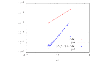
Figure 1: Scaling of $|\Delta H|$ and $|\Delta\tilde{H}|=|\Delta H+\Delta(\delta H)|$ with $\delta\tau$ at fixed $\mu=0.2$, $m=10$ and $k=10$.

It is also instructive to look at the scaling of $\Delta H$ with the trajectory length $\tau$. The conservation of the shadow Hamiltonian implies $\Delta H=-\Delta(\delta H)$, and again, by rewriting $\delta H$ using eq. 2.17 one gets

$$\Delta H=-\frac{\delta\tau^{2}}{72}\Delta\left(\left|{\mathcal{F}}_{1}\right|^{2}+\frac{\left|{\mathcal{F}}_{2}\right|^{2}}{4m^{2}}+\frac{\left|{\mathcal{F}}_{\rm G}\right|^{2}}{16m^{2}k^{2}}\right)\;,$$ (4.23)

up to $O(\delta\tau^{4})$. For one given, thermalized, initial configuration, the quantities on the two sides of the above equation are compared as a function of $\tau$ for two different values of $\delta\tau$ in the two upper panels of Fig. 2, while in the lower panel the quantity $\Delta H/\delta\tau^{2}$ is plotted. As suggested by eq. 4.23 such ratio is independent from the step-size (up to $O(\delta\tau^{2})$), since the same underlying continuous Hamilton equations with the same initial conditions are being discretized in the two cases.

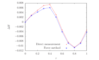
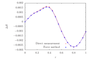
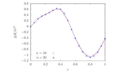
Figure 2: Comparison of the Hamiltonian violations computed directly and using the r.h.s. of eq. 4.23 as a function of the trajectory length and for different time-steps (upper-left: $\delta\tau=1/10$, $m=10$, $k=10$, upper-right: $\delta\tau=1/20$, $m=10$, $k=10$). The lower panel shows the data in the upper ones, for the “Force method” (i.e., r.h.s. of eq. 4.23) rescaled by $\delta\tau^{2}$). In all cases $V=16^{4}$, $\beta=2.2$, $m_{0}=-0.72$ and $\mu=0.2$.

4.2 Testing estimates of the acceptance

The previous tests serve the purpose of checking our computation of $\delta H$ up to $O(\delta\tau^{4})$. Here we want to assess how robust the estimates of the acceptance using $\delta H$ are. It is by modeling such expressions that we will be able to predict the efficiency of a simulation for a given choice of the parameters $\mu,\,n,\,m$ and $k$.

We can compare four different estimates of the acceptance:

• is obtained by trivially counting the number of accepted configurations (’Measurement’ in Fig. 3),

• requires measuring ${\rm Var}(\Delta H)$, which is then plugged into eq. 3.18 (’$\Delta H$ method’ in Fig. 3),

• instead of $\Delta H$ one measures the quantity on the r.h.s. of eq. 4.23 and its variance, which is then inserted in eq. 3.18 replacing ${\rm Var}(\Delta H)$ (’Forces method 2’ in Fig. 3),

• similarly to the estimate in $iii$, one replaces ${\rm Var}(\Delta H)$, in eq. 3.18 with the r.h.s. of eq. 3.21. Notice that in this case the variance is computed not only over the trajectories (as in $ii$ and $iii$), but also over the inner trajectory steps. This estimate (’Forces method 1’ in Fig. 3), is therefore expected to be the most reliable.

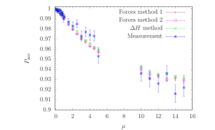
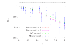
Figure 3: Comparison of the four different estimates of the acceptance described in the text as a function of the parameter $\mu$. Results refer to a $4^{4}$ lattice at $\beta=2.2$ and $m_{0}=-0.72$. We fixed $n=4$, $m=k=10$ and we ran $O(10^{3})$ trajectories of length 1 at each value of $\mu$. On the left the full range of $\mu$ explored, on the right a zoom of the area $0<\mu\leq 1$.

From Fig. 3 one concludes that, for large values of $P_{\rm acc}$, all estimates agree quite well with the measured acceptance within its errors. Also, they vary in a very smooth way, which suggests that the estimates are quite stable, and $O(10^{3})$ trajectories (as used for the figure) are enough to obtain reliable values. In the following we will use the estimate $iv$ from the list above.

4.3 Results and modelling of the data

The key observation in the proposed approach is that the variances in eq. 3.21 are functions of $\mu$ only, at fixed physical parameters (quark masses, gauge coupling and volume). We plot such variances as a function of the Hasenbusch mass-parameter $\mu$ for a $32^{4}$ lattice at $\beta=2.2$ and $m_{0}=-0.72$ in Fig. 4. These results have been obtained for $n=15$, $m=8$ and $k=10$ fixed, but in principle we could have combined results for different choices of such algorithmic parameters, as they should not affect the variances.

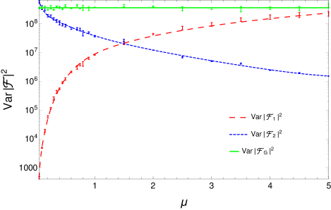
Figure 4: Variances of the forces as a function of the mass preconditioning parameter from a set of simulations at $\beta=2.2$, $m_{0}=-0.72$ and $V=32^{4}$. Curves only serve to guide the eye.

One can see that the variance of the gauge force is independent from $\mu$, as expected, whereas for ${\cal{F}}_{1}$ and ${\cal{F}}_{2}$ a region of weak dependence, for large values of $\mu$ and a region of strong dependence for small ones can be clearly identified. The interesting region for us is the one at small $\mu$, since there the hierarchy of the forces is consistent with the nested scheme adopted for the integrator (see remarks in Sect. 2.2).

Although a precise theoretical prediction on the functional form describing the dependence of such variances on $\mu$ is lacking, for small values of $\mu$ (say $\mu\lesssim 1$) one can use simple polynomial fits and impose a few reasonable constraints as the vanishing of ${\rm Var}(\left|{\mathcal{F}}_{1}\right|^{2})$ for $\mu=0$ and, following [21], a rapid growth of ${\rm Var}(\left|{\mathcal{F}}_{2}\right|^{2})$ for values of $\mu$ compensating for the quark mass (i.e., $\mu\simeq-(m_{0}-m_{\rm c})$, with $m_{\rm c}$ the critical value of the bare quark mass). Similar considerations can be used for the fit ansätze of the $\#{\rm MVM}_{i}(\mu)$ functions. We therefore adopt the following parameterizations:

$${\rm Var}(\left|{\mathcal{F}}_{1}\right|^{2})(\mu) = a\mu+b\mu^{2}+c\mu^{3}\;,$$ (4.24)

$${\rm Var}(\left|{\mathcal{F}}_{2}\right|^{2})(\mu) = \frac{a+b\mu+c\mu^{2}}{(\mu+m_{0}-m_{\rm c})^{2}}\;,$$ (4.25)

$${\rm Var}(\left|{\mathcal{F}}_{\rm G}\right|^{2})(\mu) = a\;,$$ (4.26)

$$\#{\rm MVM}_{1}(\mu) = a+b\mu\;,$$ (4.27)

$$\#{\rm MVM}_{2}(\mu) = \frac{a+b\mu+c\mu^{2}}{(\mu+m_{0}-m_{\rm c})^{2}}\;,$$ (4.28)

where of course the fit parameters $a,\,b$ and $c$ are independent for each of the quantities above. Notice that we include both even and odd terms in $\mu$ since the splitting we use is not invariant under $\mu\leftrightarrow-\mu$ (see Sect. 2.2). The fits provide good descriptions of the data with reasonable $\chi^{2}/d.o.f$ values. We stress however that any other parameterization reproducing the data would be equally good for the present purposes. In principle one could even decide to mimimize the algorithmic cost on a finite (fine) set of $\mu$ values, which would completely bypass the problem of modelling the results through smooth functional forms. At fixed quark mass, we will compare the two approaches and show that the choice does not significantly affect the final estimates, which gives us confidence on the chosen parameterizations. The advantage of modelling the data is that one can simultaneously fit the dependencies on $\mu$ and on the quark mass, which helps stabilizing the results when different sets of $\mu$ values have been considered for different quark masses. That is precisely our case. While for $m_{0}=-0.72$ we performed a rather fine scan in $\mu$, for $m_{0}=-0.735$ and $m_{0}=-0.75$ we ran simulations on a reduced set of $\mu$ values only (the lattice volume is fixed to $32^{4}$ at $\beta=2.2$, where $m_{\rm c}=-0.7676(2)$). In order to account for the quark mass dependence we promote some of the coefficients in the fit-forms above to functions of the bare subtracted quark mass and finally use:

$${\rm Var}(\left|{\mathcal{F}}_{1}\right|^{2})(\mu,m_{0}) = \frac{a\mu+b\mu^{2}+c\mu^{3}}{(m_{0}-m_{\rm c})^{2}}\;,$$ (4.29)

$${\rm Var}(\left|{\mathcal{F}}_{2}\right|^{2})(\mu,m_{0}) = \frac{a+b\mu+c\mu^{2}}{(\mu+m_{0}-m_{\rm c})^{2}}\;,$$ (4.30)

$${\rm Var}(\left|{\mathcal{F}}_{\rm G}\right|^{2})(\mu,m_{0}) = a\;,$$ (4.31)

$$\#{\rm MVM}_{1}(\mu,m_{0}) = \frac{a+b(m_{0}-m_{\rm c})+c\mu}{(m_{0}-m_{\rm c})^{2}}\;,$$ (4.32)

$$\#{\rm MVM}_{2}(\mu,m_{0}) = \frac{a+b\mu+c\mu^{2}}{(\mu+m_{0}-m_{\rm c})^{2}}\;.$$ (4.33)

The resulting fits are shown in Fig. 5.

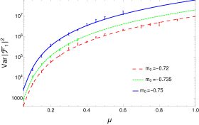
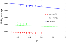
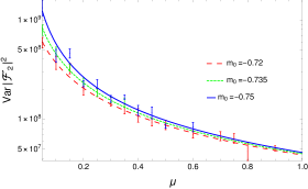
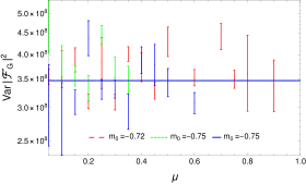
Figure 5: Left column: global fits to the forces’ variances as a function of $\mu$ for three different quark masses. Right column: global fits to the average number of matrix-vector multiplications per step in the computation of the fermionic forces vs $\mu$ and for $m_{0}=-0.72$, $-0.735$ and $-0.75$. The inverse gauge coupling $\beta$ is fixed to $2.2$ and $V=32^{4}$.

4.4 Cost predictions and verifications

Having now smooth functions of $\mu$ describing the variances in eq. 3.21 and the $\#$MVM_i in eq. 3.22, we plug the first in eq. 3.18 and then in the denominator of the r.h.s. of eq. 3.20 and the second in the numerator of the same expression, to obtain the Cost in closed form as a function of $n\;,m\;,k$ and $\mu$. At this point we minimize such function using Mathematica, under the additional constraint $P_{\rm acc}\gtrsim 0.75$, since for example the Creutz formula we used is valid in principle for large acceptances only. We further fix $k=10$ in order to reduce the parameter space for the minimization. The choice may be conservative, but since $k$ controls the frequency of the computation of the gauge force, which is very cheap, we do not expect large gains in optimizing this parameter.

What we obtain are level curves as the ones shown in Fig. 6. One can see that the minima are rather broad, especially as a function of $\mu$.

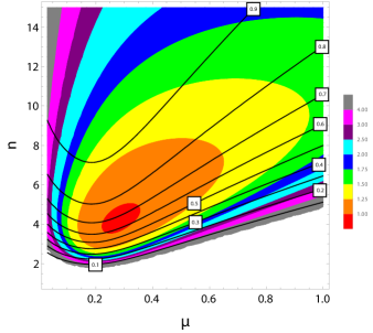
Figure 6: Slices of the Cost function at fixed $m=3$ and $k=10$ as a function of $\mu$ and $n$ (left) and at fixed $n=5$ and $k=10$ as a function of $\mu$ and $m$ (right). Solid lines represent constant acceptance curves. The cost is expressed relatively to the minimum. $\beta=2.2$, $m_{0}=-0.72$ and $V=32^{4}$.

Since we have the full Cost function (not just the minimum), we can compare predictions to actual simulations. We do that at fixed $n$, $m$ and $k$ (those corresponding to the minimum for the cost) because we are mostly interested in checking, a-posteriori, the assumptions made in fitting the dependencies on $\mu$ as described in the previous Section. In Fig. 7 we compare predictions obtained either by using the variances and average numbers of matrix-vector multiplications measured at specific values of $\mu$ (so without any fitting) or by using the parameterized forms, to actual simulations.

Figure 7: Comparison of the Cost between direct simulations and our final predictions. For the second we either used measurements at fixed values of $\mu$ (“rescaled data” in the plot) or we used fit results (“Fit prediction”). $n$, $m$ and $k$ are fixed to $5$, $3$ and $10$ respectively (again, $\beta=2.2$, $m_{0}=-0.72$ and $V=32^{4}$). Each simulation consists of about 1000 molecular dynamics units (MDU).

We see that in all cases the agreement is rather good, over a region where the cost changes by a factor of about three.

Finally, in Fig. 8 we compare our prediction for the dependence of the cost on the quark mass, to direct simulations. In this case we always fix the algorithmic parameters to the obtained minimum as we change $m_{0}$, again with the constraint $P_{\rm acc}\gtrsim 0.75$. Notice that the leftmost point corresponds to a value of $m_{0}-m_{\rm c}$ smaller than the ones previously considered in this paper and therefore the comparison provides a check of the functional dependencies on the quark mass that we have introduced in the previous Section. The agreement is quite satisfactory, and always within two combined sigmas, over a large range of cost values and that gives us confidence on the accuracy of the proposed method. More important than the discrepancy between simulations and predictions in units of combined standard deviations is actually their relative difference, which is 10% at most, so the predictions are indeed quite precise. As a final remark we point out that the dependence of the cost on the bare subtracted quark mass turns out to be consistent with a $1/(m_{0}-m_{\rm c})$ behavior.

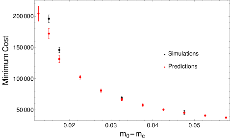
Figure 8: Cost from direct simulations and as predicted within our approach as a function of the bare subtracted quark mass. The algorithmic parameters at each point are chosen such that the cost is minimized (as usual $\beta=2.2$ and $V=32^{4}$). For each simulation we ran between 500 and 1000 MDU.

5 Conclusions

We presented a simple and general method to optimize the parameters of the integrators and those entering the determinant splitting in HMC simulations of lattice gauge theories. The main observation is that shadow Hamiltonians and Poisson brackets provide a clear way to separate the dependence of (e.g.) the violations of the energy (Hamiltonian) conservation on algorithmic and integrator parameters. The dependence on the latter is explicit, whereas that on the first is implicit in the arguments of the Poisson brackets. The idea has already been used in the past to optimize integrators, but we have extended it here in order to simultaneously optimize the algorithm (i.e., tuning the Hasenbusch mass $\mu$, in the case considered), by showing that the dependence of the Poisson brackets on the algorithmic parameters is rather smooth and can be easily parameterized. We looked at a simple case (Omelyan second order integrator, with $\alpha=1/6$, one level of Hasenbusch splitting), but more complicated ones can be straightforwardly considered, at the cost of computing Poisson brackets and model their dependence on the parameters defining the specific factorization of the quark determinant.

The considered case is however relevant as a significant amount of data is available within that setup in the framework of non-perturbative studies of strongly interacting extensions of the Standard Model. Those are becoming precise studies and simulations are getting computationally expensive, therefore it is crucial to be able to re-utilize existing results in order to optimize the efficiency of the algorithms. Since such an optimization may in principle be different for each model, a reliable and inexpensive way to do it, as the one proposed here, is highly desirable.

We indeed found a very satisfactory agreement (at the ten-percent level) between the cost predictions from our method and actual results from simulations.

Acknowledgements. We thank Ari Hietanen and Martin Hansen for help and discussions in the initial phase of the project. We wish to thank Tony Kennedy for useful discussions. This work was supported by the Danish National Research Foundation DNRF:90 grant and by a Lundbeck Foundation Fellowship grant number 2011-9799. Local computational facilities used in this work were provided by the DeIC national High Performance Computing (HPC) centre at University of Southern Denmark (SDU), funded by SDU and the Danish e-infrastructure Cooperation (DeIC). A.B. acknowledges support through the Spanish MINECO project FPA2015-68541-P, the Centro de Excelencia Severo Ochoa Programme SEV-2016-0597 and the Ramón y Cajal Programme RYC-2012-10819.

References

- [1] S. Duane, A. D. Kennedy, B. J. Pendleton and D. Roweth, Phys. Lett. B 195 (1987) 216.
- [2] M. Hasenbusch, Phys. Lett. B 519 (2001) 177, [hep-lat/0107019].
- [3] M. Lüscher, Comput. Phys. Commun. 165 (2005) 199, [hep-lat/0409106].
- [4] M. A. Clark and A. D. Kennedy, Phys. Rev. Lett. 98 (2007) 051601, [hep-lat/0608015].
- [5] I. P. Omelyan, I. M. Mryglod, and R. Folk, Comput. Phys. Commun. 151 (2003) 272.
- [6] T. Takaishi and P. de Forcrand, Phys. Rev. E 73 (2006) 036706, [hep-lat/0505020].
- [7] C. Urbach, K. Jansen, A. Shindler and U. Wenger, Comput. Phys. Commun. 174 (2006) 87, [hep-lat/0506011].
- [8] M. A. Clark, A. D. Kennedy and P. J. Silva, PoS LATTICE 2008 (2008) 041 [arXiv:0810.1315 [hep-lat]].
- [9] M. A. Clark, B. Joo, A. D. Kennedy and P. J. Silva, Phys. Rev. D 84 (2011) 071502, [arXiv:1108.1828 [hep-lat]].
- [10] A. Bussone, M. Della Morte, V. Drach, M. Hansen, A. Hietanen, J. Rantaharju and C. Pica, PoS LATTICE 2016 (2016) 260 [arXiv:1610.02860 [hep-lat]].
- [11] M. A. Clark and A. D. Kennedy, Phys. Rev. D 76 (2007) 074508 [arXiv:0705.2014 [hep-lat]].
- [12] A. D. Kennedy, P. J. Silva and M. A. Clark, Phys. Rev. D 87 (2013) no.3, 034511 [arXiv:1210.6600 [hep-lat]].
- [13] M. Della Morte et al. [ALPHA Collaboration], Comput. Phys. Commun. 156 (2003) 62, [hep-lat/0307008].
- [14] M. Luscher, arXiv:1002.4232 [hep-lat].
- [15] M. Creutz, Phys. Rev. D 38 (1988) 1228.
- [16] S. Gupta, A. Irback, F. Karsch and B. Petersson, Phys. Lett. B 242 (1990) 437.
- [17] M. A. Clark, B. Joo, A. D. Kennedy and P. J. Silva, PoS LATTICE 2010 (2010) 323, [arXiv:1011.0230 [hep-lat]].
- [18] H. B. Meyer, H. Simma, R. Sommer, M. Della Morte, O. Witzel and U. Wolff, Comput. Phys. Commun. 176 (2007) 91, [hep-lat/0606004].
- [19] M. Della Morte et al. [ALPHA Collaboration], JHEP 0807 (2008) 037, [arXiv:0804.3383 [hep-lat]].
- [20] L. Del Debbio, A. Patella and C. Pica, Phys. Rev. D 81 (2010) 094503, [arXiv:0805.2058 [hep-lat]].
- [21] L. Del Debbio, L. Giusti, M. Luscher, R. Petronzio and N. Tantalo, JHEP 0602 (2006) 011, [hep-lat/0512021].