Zipf and Heaps laws from dependency structures in component systems

Abstract

Complex natural and technological systems can be considered, on a coarse-grained level, as assemblies of elementary components: for example, genomes as sets of genes, or texts as sets of words. On one hand, the joint occurrence of components emerges from architectural and specific constraints in such systems. On the other hand, general regularities may unify different systems, such as the broadly studied Zipf and Heaps laws, respectively concerning the distribution of component frequencies and their number as a function of system size. Dependency structures (i.e., directed networks encoding the dependency relations between the components in a system) were proposed recently as a possible organizing principles underlying some of the regularities observed. However, the consequences of this assumption were explored only in binary component systems, where solely the presence or absence of components is considered, and multiple copies of the same component are not allowed. Here, we consider a simple model that generates, from a given ensemble of dependency structures, a statistical ensemble of sets of components, allowing for components to appear with any multiplicity. Our model is a minimal extension that is memoryless, and therefore accessible to analytical calculations. A mean-field analytical approach (analogous to the “Zipfian ensemble” in the linguistics literature) captures the relevant laws describing the component statistics as we show by comparison with numerical computations. In particular, we recover a power-law Zipf rank plot, with a set of core components, and a Heaps law displaying three consecutive regimes (linear, sub-linear and saturating) that we characterize quantitatively.

I Introduction

Several physical, biological, and artificial systems are modular and can be partitioned in well-defined basic components, revealing essential features of their architecture. For example, genomes can be regarded as sets of genes, operating systems as sets of packages, texts as sets of words van Nimwegen (2003); Gherardi et al. (2013); Pang and Maslov (2013); Altmann and Gerlach (2016); Mazzolini et al. (2017). A system showing this simple modular structure can be considered as a specific collection of partitions of elementary components (a “component system”), whose statistical properties may reveal information on the system’s generative mechanisms. For example, books in a linguistic corpus composed by $N$ words (the total number of “tokens” in quantitative-linguistics language) are partitions of $N$ elements in component classes identified by the different words, or “types”. These partitions, and their statistical properties, are generally an extension of the classic partitions intensively studied in probability Pitman (1995) as well as in statistical mechanics, for example related to the equilibrium statistics of particles in energy states Leinaas and Myrheim (1977), or to non-equilibrium site occupancy in driven diffusive systems Evans and Hanney (2005), or resulting from stochastic processes based on duplication-innovation mechanisms Angelini et al. (2010); Cosentino Lagomarsino et al. (2009).

The representation of complex systems as component systems reveals a variety of quantitative laws, which, intriguingly, are often conserved across very different systems. Prominent examples are Zipf’s law, concerning the power-law distribution of component frequencies Zipf (1935); Newman (2005); Mitzenmacher (2004); Lotka (1926); Huynen and van Nimwegen (1998); Axtell (2001), and the sublinear scaling of the number of different component classes with system size, often referred to as Heaps’ law Herdan (1960); Heaps (1978); Powers (1998); Cosentino Lagomarsino et al. (2009). The analysis of these laws has a long tradition in quantitative linguistics Altmann and Gerlach (2016); Zipf (1935). Several mechanisms of text generation, based on different hypotheses on the fundamental structures or principles of natural language, have been proposed to explain these statistical patterns i Cancho and Solé (2003); Zanette and Montemurro (2005); Gerlach and Altmann (2013). Analogously, in genomics, the coarse-grained view of genomes as component systems reveals emergent quantitative invariants pointing to relevant underlying evolutionary and architectural properties of genomes Koonin (2011); Grilli et al. (2012a); Lobkovsky et al. (2013); Maslov et al. (2009); Pang and Maslov (2013); van Nimwegen (2003).

Scale invariance (and universality), suggested by the presence of Zipf’s law, may be a natural consequence of criticality Mora and Bialek (2011), either due to evolutionary tuning or self-organization Bak et al. (1987); Hidalgo et al. (2014), as is well understood via the renormalization group in statistical mechanics. However, more and more often scale-free features in different contexts have been recognized as a possible consequence of stochastic processes based on specific features, such as preferential attachment Newman (2005); Mitzenmacher (2004) or a history-dependent entropic reduction of the accessible states Hanel and Thurner (2011); Corominas-Murtra et al. (2015). The plethora of possible mechanisms that can generate these pervasive statistical patterns raises questions concerning their true origin and their robustness Sornette (2006).

Typically, these proposed mechanisms do not explicitly take into account the functional specificities of single components, nor their functional dependencies, nor the possible synergy and conflicts between components. These interactions are essential in most empirical systems. For example, the importance of this aspect is clear in operating systems (or other large software projects), where a package performs a specific function and typically requires the presence of other components for functioning. Indeed, models based on dependency structures have emerged recently as a promising framework to rationalize component dependencies and analyze their consequences in terms of component statistics Pang and Maslov (2013). Similar dependency structures also emerge in preference prediction Heckerman et al. (2000), or for addressing causality in financial data Kenett et al. (2010).

More precisely, a dependency structure is a directed graph (most often, but not necessarily, acyclic), whose nodes are the components (e.g., Linux packages, or genes) and whose links are the dependency relations occurring between them (e.g. requirement constraints or regulatory pathways). A component depends on another if it is not functional unless the latter is present. A simple mechanism to build a component system compatible with a given dependency structure identifies a system realization (e.g., a genome or a book) with the choice of a node and all its direct and indirect dependencies Pang and Maslov (2013). This model allows to link quantitative laws of the component statistics to topological properties of the dependency structure (and hence to the generative processes sculpting it). For instance, a broad ensemble of dependency structures has the property that the number of total dependencies of each node is scale free in the limit of large system size (notice that this is a weaker condition than the power-law distribution of degrees, i.e., of only direct dependencies).

This topological property explains the fat-tailed distribution of component occurrences across realizations, both in genomes and operating systems Pang and Maslov (2013). However, since this simple model was inspired by software packages, it was developed in the restrictive case of binary (presence/absence) abundances of components. While a piece of software is either installed or absent, in most empirical component systems a component type can be present in many instances. For example, a gene is typically present in multiple copies (called paralogs) in a genome, and the same word is typically used several times in a single book.

Here, to capture this large class of component systems, we consider an extension of the model proposed in Ref. Pang and Maslov (2013) to the cases in which components can appear with arbitrary abundances. This extension is able to address the question of how dependency structures affect abundance-related features, such as Zipf’s laws and in particular Heaps’ law. The same question is not defined in the case of binary component abundances, where, for example, Heaps’ law is trivially linear.

II Model

We consider a simplified description of complex functional architectures as unordered sets of modular components. Let $\mathcal{U}$ be the set of all unique components (the universe), and let $U=\left|\mathcal{U}\right|$ denote its cardinality. A realization of this “component system” is a set $r=\left\{c_{i}\right\}$ of components $c_{i}\in\mathcal{U}$, with $i=0,\ldots,N$, where $N$ is the size of the realization. The rules for constructing a realization are specified by a network of dependencies, as we explain below.

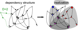
Figure 1: Illustration of the model. The model is defined by two steps. The first step creates a dependency structure by an incremental node-addition process with mean out-degree D. The second step builds realizations drawing at random $k$ precursor nodes (larger circles in figure, where $k=2$) and taking all components belonging to their forward “cones” of dependency (shaded in gray). This second step assigns multiplicities to the components appearing in each realization: the abundance of component $i$ is the number of precursors whose forward cones contain $i$. In the realization illustrated in the right panel, two precursor components (larger circles) are chosen; the nodes (components) in the light-gray regions have multiplicity 1, while those in the dark-gray region have multiplicity 2.

A dependency structure is a directed acyclic graph $\mathcal{G}$ on $\mathcal{U}$, which encodes the dependencies between the components. An edge $i\to j$ between two nodes $i$ and $j$ represents the relation “$i$ depends on $j$”. A component $i$ is said to depend on another component $j$ if $i$ is not functional without $j$. In empirical cases, such a relation can be more or less strict depending on the system; for instance it is enforced in software operating systems, where a package cannot function unless all its dependencies are installed, but not in metabolic networks, where alternative pathways can be followed to the same metabolite Fortuna et al. (2011); Maslov et al. (2009). The model assumes strict unbroken dependencies. Notice that acyclicity of $\mathcal{G}$ is not stringently necessary; however, as will be clear in the following, a cycle in $\mathcal{G}$ would behave as a single node in the model.

The topology of the dependency structure is conceptually separated from the procedure that generates realizations satisfying the dependency constraints. Here we use the ensemble of dependency structures introduced in Ref. Pang and Maslov (2013), and we define a novel method to build the realizations. Specifically, as sketched in Fig. 1, the growth process that creates the dependency network is an incremental node-addition process generating structures with power-law distributed sizes of direct and indirect dependencies (such property is crucial to reproduce Zipf’s law, see below). More specifically, let us fix an average out-degree $D\geq 1$, i.e., an average number of direct dependencies of a given component. Starting with an initial graph consisting of a single node, the full graph is built node by node, by attaching the new node to $d+1$ randomly chosen existing nodes (possibly with repetitions), where $d$ is a Poissonian random variable of mean $D-1$. The process is stopped when the network reaches the predetermined size $U$. A graph assembled with these rules is directed and acyclic, and hence a good dependency structure, as can be seen by labeling each node by the time $t=1,\ldots,U$ it was added to the network, and noticing that there can be no links $t\to t^{\prime}$ with $t<t^{\prime}$. Given a node $c$, the set $\wedge(c)\subseteq\mathcal{U}$ is defined as the set of all nodes $c^{\prime}$ such that there exists at least one directed path in $\mathcal{G}$ starting from $c$ and arriving at $c^{\prime}$. We will call the set $\wedge(c)$ the forward cone of $c$. Similarly, we define the backward cone $\vee(c)$ of $c$ as the set of all nodes $c^{\prime}$ such that there exists a path from $c^{\prime}$ to $c$. In other words, $\wedge(c)$ is the set of all components required be the (direct and indirect) dependencies of $c$, whereas $\vee(c)$ is the set of the nodes that depend (directly or indirectly) on $c$.

Once a dependency structure $\mathcal{G}$ is established, realizations of the model, i.e., sets of components, are generated by the following procedure (see also Fig. 1). Let us fix a positive integer $k$, which represents the number of “precursor” components determining a realization. The $k$ precursors $\left\{p_{j}\right\}$, $j=1,\ldots,k$, are chosen randomly and independently among the nodes of $\mathcal{G}$. Then the corresponding realization is produced by taking all components belonging to the forward cones of the precursors. To complete the model specification one needs a rule to choose the multiplicities of the components. We allow a component belonging to multiple cones to appear in multiple copies. Let us imagine that precursors are added one at a time to the realization. At the $j$-th step the existing realization $r_{j-1}$ (possibly empty, when $j=1$) is extended, by the addition of elements from the cone $\wedge(p_{j})$ of the precursor $p_{j}$:

$$r_{j}=r_{j-1}\cup\Delta_{j},\quad\Delta_{j}\subseteq\wedge(p_{j}).$$ (1)

The choice of the incrementing set $\Delta_{j}$ must be done so as to satisfy the dependency relations, i.e., $r_{j}\supseteq\wedge(p_{j})$. Doing this at every step ensures that the final realization $r_{k}$ will not have any unsatisfied dependency. Other than that, $\Delta_{j}$ is in principle unconstrained, and it may be a random variable even at fixed $p_{j}$ and $r_{j-1}$. Here we make the simplest choice

$$\Delta_{j}=\wedge(p_{j}).$$ (2)

This makes the process Markovian, in the sense that $r_{j}\setminus r_{j-1}\equiv\Delta_{j}$ is independent of $r_{j-1}$. The case $k=1$, when a realization is specified by a single precursor, reproduces the model of Pang and Maslov (2013).

III Results

Our description separates the relational constraints existing between the components, such as dependency and incompatibility, from their functional correlations, such as synergy, co-occurrence, interchangeability, conflict, and so on. For what concerns the functional correlations, our model is the simplest null model where no correlations between components are dictated, other than those arising from the dependencies. An advantage of this model is its analytical tractability. The form of Zipf’s law is basically the same as in the binary model, and the mean-field analysis parallels that in Pang and Maslov (2013). The main additional output of our extension is a non-trivial Heaps’ law, which is derived analytically below.

III.1 Zipf’s law and the occurrence-abundance relation

We now set out to compute the distribution of component abundance emerging from a set of realizations in this model, equivalent to the empirical Zipf’s law measured from a set of texts.

Given a set of $R$ realizations of a component system, the “popularity” of a component $i$ can be measured in two ways: by its abundance $a_{i}$ and by its occurrence $o_{i}$. The abundance counts the number of times that $i$ appears in all realizations (with multiplicities):

$$a_{i}=\frac{1}{kR}\sum_{r}\sum_{c\in r}\delta_{c,i}.$$ (3)

In the model, the maximum abundance of a component $i$ corresponds to drawing $i$ each time a cone is selected, for each realization. In such a case, the double sum in (3) is $kR$. Therefore, the abundance $a_{i}$ is normalized so that $0\leq a_{i}\leq 1$ (we will call $a_{i}$ the relative abundance when it is important to stress that it is an intensive quantity). The occurrence $o_{i}$ measures the fraction of realizations containing the component, regardless of its abundance:

$$o_{i}=\frac{1}{R}\sum_{r}\left[1-\prod_{c\in r}\left(1-\delta_{c,i}\right)\right].$$ (4)

With this definition, the occurrence is normalized so that $0\leq o_{i}\leq 1$.

Zipf’s law is a statement about the rank-frequency relation of components. Specifically, the frequency of a component decreases as a power of its rank $r$, $f_{r}\propto r^{-\gamma}$ (where the rank is $1$ for the most frequent component, $2$ for the second most frequent, and so on) Altmann and Gerlach (2016). The Zipf relation is expected to be independent of the number of cones $k$ (at least for large systems). In fact, the abundance $a_{i}$ of a given component in $R$ realizations constructed with $k$ cones each has the same distribution as that in $kR$ single-cone realizations, since the choices of the cones are independent. $a_{i}$ can be estimated as the probability of choosing a cone that contains $i$, which is proportional to the size $\left|\vee(i)\right|$ of the backward cone of $i$:

$$a_{i}=\frac{\left|\vee(i)\right|}{U}.$$ (5)

Let us call $\mathrm{rank}(i)$ the rank of component $i$ when all components are ranked by their abundance. Following Pang and Maslov (2013), an approximate relation can be derived between $\left|\vee(i)\right|$ and $\mathrm{rank}(i)$, which will allow to obtain an analytical estimate of Zipf’s plot. The $t$-th node in the network (the one added at the $t$-th step of the construction, when a network of size $t-1$ has been already generated) has approximately $(U/t)^{D}$ nodes that depend on it. This result can be obtained by writing an equation stating that the backward cone of the $t$-th node is the union of the backward cones of all the nodes that, at later times $t^{\prime}$, will directly attach to the $t$-th node. Neglecting the intersections between these cones allows one to write the recursion

$$\left|\vee(t)\right|=1+\sum_{t^{\prime}=t+1}^{U}\frac{D}{t^{\prime}}\left|\vee(t^{\prime})\right|,$$ (6)

where the factor $D/t^{\prime}$ estimates the probability that the $t^{\prime}$-th node attaches to the $t$-th node (with a slight abuse of notation, we write $\wedge(t)$ and $\vee(t)$ for the forward and backward cones of the $t$-th node). By approximating the sum by an integral and taking a derivative with respect to $t$, one obtains a differential equation that is solved by $\left|\vee(t)\right|=(U/t)^{D}$.

For small $t$, however, $(U/t)^{D}$ is greater than the size of the network $U$. In fact, the relation can hold only down to a cutoff $t_{\mathrm{min}}$, which can be estimated by the condition that the whole network depends on the $t_{\mathrm{min}}$-th node, i.e., $(U/t_{\mathrm{min}})^{D}=U$, which gives $t_{\mathrm{min}}=U^{1-1/D}$. For any node below $t_{\mathrm{min}}$, the size of its backward cone is $\approx U$:

$$\left|\vee(t)\right|\approx\begin{dcases}U\quad&t<U^{1-1/D}\\ \left(U/t\right)^{D}&t\geq U^{1-1/D}\end{dcases}$$ (7)

Equations (5) and (7) imply that if node $i$ is the $t$-th node in the network growth process, then $t=\mathrm{rank}(i)$. (This identification does not hold for the first $U^{1-1/D}$ components, but this does not influence the result since the size of their backward cones are equal in this approximation.) Therefore, one obtains

$$a_{i}\approx\begin{dcases}1\quad&\mathrm{rank}(i)<U^{1-1/D}\\ \mathrm{rank}(i)^{-D}U^{D-1}&\mathrm{rank}(i)\geq U^{1-1/D}.\end{dcases}$$ (8)

This relation has the form of a Zipf power-law (with exponent $-D$) with an initial “core set” consisting of $U^{1-1/D}$ components having similar abundances. Figure 2(a) compares the analytical form (8) with the results of simulations, showing good accord, especially in the behavior of the fat tail. The transition between the core and the tail, instead, is less sharp than predicted. This is due to the fact that the relation $\left|\vee(t)\right|=(U/t)^{D}$ starts to break down before reaching $U$, and saturates more smoothly than in the approximation made above. Importantly, the relation between rank and relative abundance does not depend on the number of cones $k$, in accord with the foregoing prediction.

Contrary to the binary case discussed in Ref. Pang and Maslov (2013), where abundance and occurrence are the same quantity [as shown by Eq. (9) below], the rank-occurrence and rank-abundance relations in our model are different in general. Figure 2(b) shows that the Zipfian plot for the occurrence has a similar appearance to the usual one, but with a larger and larger core as $k$ increases. When plotted as a probability distribution function in linear scale, the rank-occurrence relation has a characteristic U shape Koonin and Wolf (2008); Touchon et al. (2009), that highlights a subset constituted by a large number of rare components and a subset of components shared by a large fraction of realizations, usually referred to as the “cloud” and “core” sets respectively Lobkovsky et al. (2013). How these features are related to Zipf’s law is explored in detail in Ref. Mazzolini et al. (2017).

The occurrence-abundance relation predicted by our model turns out to be universal (or “null”), meaning that it is insensitive to the explicit form of Zipf’s law, to the detailed structure of the network, and even to the size $U$ of the component universe. In fact, we show here that a simple probabilistic argument gives a relation that is consistent with simulations of the full model. In the limit of large $R$, we can assume that the occurrence of a component $i$ is equal to the probability of choosing $i$ at least once in a single realization: $o_{i}=1-(1-a_{i})^{k}$, hence

$$a_{i}=1-\left(1-o_{i}\right)^{1/k}.$$ (9)

For realizations with a single precursor ($k=1$), abundance and occurrence are equal. As $k$ increases, more and more components (with larger and larger occurrence) assume small abundances. In the large-$k$ limit, all components have zero (relative) abundance, except those with occurrence 1. Figure 2(c) shows that a scatterplot of abundance versus occurrence in simulations perfectly matches the theoretical prediction (9). The figure shows results for a single choice of $D$ and $U$, but we checked that these parameters have no effect on the curves.

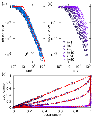
Figure 2: Simulations match the analytical prediction for the distribution of total abundance in a set of realizations (empirical Zipf’s law) and for the abundance-occurrence relation. (a) Rank-plot of component abundances. (b) Rank-plot of component occurrences. (c) Scatterplot of the abundance (y axis) versus the occurrence (x-axis) of each component. Colored symbols are results of simulations ($1000$ realizations) with varying number of precursors $k$, the dashed lines are the analytical prediction. (Parameters: $U=1000$, $D=1.5$.)

III.2 Analytical form of Heaps’ law

We now ask about the change of the typical number of distinct components with realization size. The calculation of the number $F(N)$ of unique components in a realization of size $N$ can be performed in a mean-field approximation, where the correlations between nodes are neglected. We consider a process where a realization is generated by extracting $N$ nodes independently. The full model adds entire dependency cones at once. However, one expects that the size $N$ of a realization scales linearly with the number of cones $k$, and we have verified with simulations that this is indeed the case. The assumption of independent extractions makes our mean-field approach to evaluate Heaps’ law analogous to the so-called “Zipfian ensemble” of quantitative linguistics, in which realizations are generated through random extractions of components with probabilities proportional to their frequencies Mazzolini et al. (2017); van Leijenhorst and Van der Weide (2005); Font-Clos and Corral (2015), or through a Poisson process in which component frequencies establish their arrival rates Eliazar (2011). In this framework, Heaps’ law is the natural result of the heterogeneity in component frequencies described by Zipf’s law.

The probability

$$p(t)=\frac{1}{\Omega}\left|\vee(t)\right|$$ (10)

of drawing the node $t$ is proportional to the size $\left|\vee(t)\right|$ of the node’s backward cone. In a continuous approximation, the normalization $\Omega$ can be fixed by the condition $\int_{0}^{\infty}p(t)\;\mathrm{d}t=1$, which yields

$$\Omega=U\frac{DU^{1-1/D}-1}{D-1}.$$ (11)

Note that $\Omega>U$ whenever $U>1$ and $D>1$.

Let $p_{1}(t,n)$ be the probability that the $t$-th node in the network is drawn for the first time when the system being constructed has size $n$:

$$p_{1}(t,n)=p(t)\left[1-p(t)\right]^{n-1}.$$ (12)

A mean-field estimate of $F$ can then be obtained as

$$F(N)=\sum_{n=1}^{N}\sum_{t=1}^{U}p_{1}(t,n)\approx\int_{0}^{U}\!\!\mathrm{d}t\sum_{n=1}^{N}p_{1}(t,n)$$ (13)

The geometric sum in $n$ gives simply the probability $1-[1-p(t)]^{N}$ that the $t$-th node has been drawn at least once after $N$ steps. The mean-field expression for Heaps’ law is then given by the following integral:

$$\begin{split}F(N)&=\int_{0}^{U}\!\!\mathrm{d}t\left\{1-\left[1-p(t)\right]^{N}\right\}\\ &=U-U^{1-1/D}\left(1-\frac{U}{\Omega}\right)^{N}-\mathcal{I}(N),\end{split}$$ (14)

where the first term ($U$) comes from the integral of $1$, and the second and third terms are the contributions of the two regions in (7). The remaining integral

$$\mathcal{I}(N)=\int_{U^{1-1/D}}^{U}\!\!\mathrm{d}t\left[1-\frac{1}{\Omega}\left(\frac{U}{t}\right)^{D}\right]^{N}$$ (15)

can be evaluated with the change of variables $z=(U/t)^{D}/\Omega$, which gives

$$\mathcal{I}(N)=\frac{U}{D}\Omega^{-1/D}\int_{1/\Omega}^{U/\Omega}(1-z)^{N}z^{-1-1/D}\mathrm{d}z.$$ (16)

By remembering that the primitive of $(1-z)^{\alpha}z^{\beta}$ is $z^{\beta+1}\;_{2}F_{1}(-\alpha,\beta+1,\beta+2,z)/(\beta+1)$, where ${}_{2}F_{1}$ is the Gauss hypergeometric function, one finally obtains

$$\begin{split}F(N)&=U-U^{1-1/D}\left(1-\frac{U}{\Omega}\right)^{N}\\ &\phantom{=}-\;_{2}F_{1}\left(-N,-\frac{1}{D},1-\frac{1}{D},\frac{1}{\Omega}\right)U\\ &\phantom{=}+\;_{2}F_{1}\left(-N,-\frac{1}{D},1-\frac{1}{D},\frac{U}{\Omega}\right)U^{1-1/D}.\end{split}$$ (17)

The hypergeometric function ${}_{2}F_{1}(-N,\cdot,\cdot,\cdot)$ is real when $N$ is an integer. Fig. 3 shows that the analytical mean-field expression (17) nicely matches the results of numerical simulations of the model.

III.3 Linear, sublinear, and saturation regimes of Heaps’ law

If a realization is constructed by incremental addition of randomly chosen components, one expects $F(N)$ to be approximately linear for small $N$, as it is unlikely to draw the same component twice. Intuitively, the probability to do so increases with $N$, up to a point where approximately all components in the universe will have been included, and $F(N)$ will saturate to $U$. For instance, this is the behavior observed empirically for the species-area relationship in ecology Rosindell and Cornell (2007); Grilli et al. (2012b); O’Dwyer and Cornell (2017). This behavior becomes apparent by plotting $F(N)$ in log-log scale [see Fig. 3(a)]. There emerge three distinct regimes: a linear increase for small $N$, a saturation to $U$ for large $N$, and an intermediate regime where the sub-linear increase of $F(N)$ appears to be well described by a power law. Two transition points can be identified, $N_{\mathrm{c}}$ and $N_{\mathrm{s}}$, respectively at the crossover between the linear and the sub-linear regimes, and at the onset of saturation. We collect here a few analytical estimates and observations.

It is clear from expression (14) that, since $p(t)>0$ for a finite universe,

$$\lim_{N\to\infty}F(N)=U.$$ (18)

This is a consequence of the definition of the model, whereby $F(N)$ is monotonic by construction and $F(N)\leq U$. However, this limit is not apparent from the final formula (17). What happens is that the (essential) singularities of the two hypergeometric functions cancel out in the large-$N$ limit. This makes it difficult to compute values of $F(N)$ numerically in this regime (see below).

An estimate of the point $N_{\mathrm{s}}$ where the saturation regime sets in can be obtained from (14). The term with $(1-U/\Omega)^{N}$ is significantly different from zero when $U/\Omega\lesssim 1/N$, i.e., when $N\lesssim\Omega/U$. The integral $\mathcal{I}(N)$, instead, can be evaluated for large $N$ in a saddle point approximation. The integrand [Eq. (15)] attains its minimum at $t=U$, where it is equal to $(1-1/\Omega)^{N}$; hence, it is significantly different from zero when $N\lesssim\Omega$. Therefore, both $N$-dependent terms in (14) are negligible when $N\gtrsim N_{\mathrm{s}}=\Omega$, where $\Omega$ is given by (11).

The small-$N$ behavior at finite $U$ can be obtained in principle from Eq. (14) as well, by expanding in $N$ before performing the integral in $\mathcal{I}(N)$. However, it is easier to analyze the onset of sub-linearity in the large-$U$ regime, by expanding Eq. (17) in powers of $1/U^{1-1/D}$. This can be done by using the definition of the hypergeometric function:

$$_{2}F_{1}(a,b,c,z)=\sum_{k=0}^{\infty}\frac{(a)_{k}(b)_{k}}{(c)_{k}k!}z^{k},$$ (19)

where $(\alpha)_{k}=\alpha(\alpha+1)(\alpha+2)\cdots(\alpha+k-1)$ is the Pochhammer symbol. The two terms of the form ${}_{2}F_{1}(...)$ in (17) can be expanded in powers of $z$; Eq. (19) shows that the term of order $z^{j}$ in such an expansion is a polynomial of order $j$ in $N$. The same property holds for the small-$z$ expansion of the first $N$-dependent term in (17), of the form $(1-z)^{N}$. It is then easy to see, by keeping track of the analytical and non-analytical powers of $U$, that in the limit $U\to\infty$ the only non-vanishing term is $N$, and Heaps’ law reduces to the identity

$$\lim_{U\to\infty}F(N)=N.$$ (20)

A linear onset is expected for small $N$ even when $U$ is finite. Performing explicitly the expansion to first order in $U^{-1+1/D}$ yields

$$F(N)\approx N-\frac{1}{2}N(N-1)\frac{2(D-1)^{2}}{D(2D-1)}U^{-1+1/D}.$$ (21)

The crossover point $N_{\mathrm{c}}$ separating the linear and sub-linear regimes can be estimated by the point where (21) reaches its maximum:

$$N_{\mathrm{c}}=\frac{D(2D-1)}{2(D-1)^{2}}U^{1-1/D}.$$ (22)

This expression is expected to become inaccurate when $D\approx 1$ (where in fact it diverges), because all terms of order $U^{-j+j/D}$ with $j>1$, which are neglected in (21), approach constants for $D\to 1$.

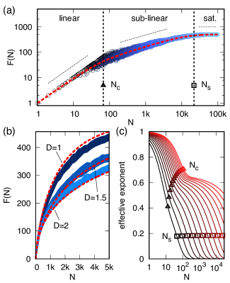
Figure 3: The model reproduces the characteristic three-regimes structure of Heaps’ law. (a) The number of distinct components $F(N)$ of a realization as a function of realization size $N$ (in log-log scale). The colored circles are simulations, lighter shades of blue correspond to larger numbers $k$ of precursors ($k$ ranges from $1$ to $3000$). The red dashed lines are the analytical prediction (17). The area of the solid curves represents the $90\%$ variability interval. (b) The same plot of $F(N)$, in linear scale, for three values of the mean out-degree $D$: $1$ (dark blue), $1.5$ (blue) and $2$ (light blue). (Parameters: $U=500$, $D=2$, $13000$ realizations.) (c) Effective exponent versus realization size for for increasing values of $U$ (black- to red-colored lines, ranging logarithmically from $U=10$ to $U\approx 6000$). Triangles correspond to the analytical estimate of $N_{\mathrm{c}}$, which captures well the transition to a plateau region. The analytical estimate of $N_{\mathrm{s}}$ (squares) corresponds to an approximately constant effective exponent.

In order to identify more visually the transition points from the data, one can plot the effective exponent

$$\gamma_{\mathrm{eff}}(N)=\frac{\mathrm{d}\log F(N)}{\mathrm{d}\log N}$$ (23)

which is easily computed from numerical data as a discrete derivative. $\gamma_{\mathrm{eff}}(N)$ measures the apparent exponent that is obtained by approximating the function $F(N)$ locally by a power-law $N^{\gamma_{\mathrm{eff}}}$. Figure 3(c) shows the effective exponent for a range of values of $U$. For small $U$, the regimes are somewhat intertwined, and no sharp transitions appear. For larger $U$, $\gamma_{\mathrm{eff}}$ shows three plateaux, corresponding to $\gamma_{\mathrm{eff}}=1$, $\gamma_{\mathrm{eff}}=0$, and an intermediate value $\gamma_{\mathrm{eff}}=\gamma$. An approximate value for $\gamma$ can be obtained by making the approximation $(1-\epsilon)^{N}\approx\exp(-N\epsilon)$ in Eq. (15), where $\epsilon=(U/t)^{D}/\Omega$. The integral then becomes

$$\mathcal{I}(N)\approx\left(\frac{N}{\Omega}\right)^{1/D}\left.\Gamma\left(1-\frac{1}{D},x\right)\right|^{x=N/\Omega}_{x=NU/\Omega}.$$ (24)

In the intermediate regime $N_{\mathrm{c}}\ll N\ll N_{\mathcal{s}}$ the upper incomplete gamma function $\Gamma$ only contributes a constant in $N$. Therefore from the prefactor one readily obtains $\gamma=1/D$. This same exponent can be derived in the framework of the Zipfian ensemble computations by a simple scaling argument by assuming a pure power-law behavior of $F(N)$ van Leijenhorst and Van der Weide (2005); Eliazar (2011); Lü et al. (2010).

Figure 3(c) also shows that the transition points computed above, i.e., $N_{\mathrm{c}}$ given by (22), and

$$N_{\mathrm{s}}=U\frac{DU^{1-1/D}-1}{D-1},$$ (25)

are reasonable estimates of the sizes where the two regime shifts occur. Surprisingly, the estimate of $N_{\mathrm{s}}$ turns out to correspond to an approximately $U$-independent value of the effective exponent.

III.4 Stretched exponential saturation as a phenomenological expression of Heaps’ law

As pointed out above, the asymptotically flat behavior of Heaps’ law $F(N)$ in this model results from the cancellation of two infinite contributions in the analytical formula. This subtlety makes it numerically challenging to evaluate $F(N)$, especially for large $U$ and $N$. Such a difficulty prevents the use of Eq. (17) to estimate the parameters by fitting against empirical data. However, the analytical expression (16) suggests a simple phenomenological expression, which can be useful in fits. Since the integration variable $z$ is small for large $U$, one can attempt to approximate the integrand in $\mathcal{I}(N)$ by $z^{-1-1/D}\exp(-zN)\mathrm{d}z$. In this form, the integral is similar to a representation of the stretched exponential function $\psi_{\gamma,a}(x)=\exp(-ax^{\gamma})$ in terms of exponential decays as a Laplace transform

$$\psi_{\gamma,a}(x)=\int_{0}^{\infty}P_{\gamma,a}(z)e^{-zx}\mathrm{d}z\ .$$ (26)

The asymptotic behavior of $P_{\gamma,a}(z)$ is known to be

$$P_{\gamma,a}(z)\sim z^{\gamma+1}$$ (27)

for large $z$, and an exponential decrease for small $z$ Johnston (2006). This suggests the following phenomenological expression:

$$F_{\mathrm{ph}}(N)=U\left[1-\exp\left(-aN^{\gamma}\right)\right]\ .$$ (28)

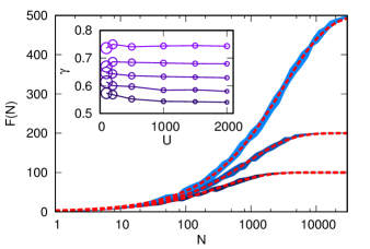
Figure 4: The stretched exponential is a good approximation of the Heaps plot generated by the model. Number of unique components ($y$ axis, in linear scale) as a function of realization size ($x$ axis, in logarithmic scale), for three different values of $U$, the size of the universe. Simulations are the solid curves (dark blue $U=100$, blue $U=200$ and light blue $U=500$; line width is the $90\%$ variability interval). The dashed red lines are the analytical prediction. (Parameters: $D=1.5$, $k$ ranging from 1 to 5000.) (Inset) The fitted stretched-exponential exponent $\gamma$ as a function of $U$. Different shades correspond to $D=1,1.25,1.5,1.75,2$, from top to bottom; point size represents errors.

Figure 4 shows that the stretched-exponential saturation, Eq. (28), is a remarkably good approximation of the simulated data. The log-linear scale reveals that the agreement is tight on the whole range of $N$. However, the phenomenological expression fails to capture the transient linear increase at small sizes (see Sec. III.3). Indeed, the small-$N$ behavior of $F_{\mathrm{ph}}$ is $F_{\mathrm{ph}}(N)\sim UaN^{\gamma}$. Interestingly, if one extracts $\gamma$ by matching the large-$z$ power-law scaling in Eq. (27) with the factor $z^{-1-1/D}$ in Eq. (16), one obtains $\gamma=1/D$, which is the same exponent that was derived from Eq. (24). Note however that the integration range in (16) is very different from the one in the integral representation (26) of $\psi_{\gamma,a}$, that is $(0,\infty)$. As a consequence, the fitted exponents $\gamma$ can deviate from the simple scaling relation $\gamma=1/D$. Altogether, these considerations suggest that it is quite surprising that the stretched exponential can be such a good approximation.

IV Discussion

It is interesting to compare the results of this positive model, where the component statistics are purely determined by component dependencies, with more null views of Heaps’ and Zipf’s laws. Our analytical computations for the rank-abundance, rank-occurrence, and Heaps’ relations were all performed in an ensemble where correlations between different components are neglected. The agreement between the results obtained in such a mean-field approximation and the numerical simulations of the full model reflects the fact that the main statistics considered are not sensitive to the correlations. In particular, the approximate stretched-exponential form of Heaps’ law is expected to hold not only for this particular positive model, but for any model yielding a Zipf law similar to Eq. (8). This observation is in agreement with the results of Ref. Mazzolini et al. (2017), where it is shown that building realizations of a component system by randomly sampling from the global frequency distribution of its components reproduces some empirical statistics of real systems to a surprising detail.

In this perspective, the positive framework established here around the concept of dependency structures introduces positive features without violating many of the null predictions of the random sampling. Understanding how the positive trends emerge from the random features is clearly crucial to determine the role played by dependencies in a given empirical system. We briefly discuss two such positive features here, leaving a more detailed investigation for future work. First, the Zipf law in Eq. (8), which is the main input of a sampling procedure Mazzolini et al. (2017), is instead a positive output of the model studied here: fixing the network of dependencies between components constrains all the main statistics regarding their abundance and occurrence, including their frequency distribution. Second, the existence of dependency relations generates nontrivial correlations between the components. These correlations can be observed, e.g., by measuring the empirical distribution of the mutual information between the occurrences of pairs of components. Let $p_{i}(x)$ be the fraction of realizations in which the component $i$ has state $x$, where $x=1$ means it is present and $x=0$ means it is absent, and let $p_{ij}(x,y)$ be the fraction of realizations in which the component $i$ has state $x$ and the component $j$ has state $y$. The mutual information between the two components, measuring how much the presence of one informs on the presence of the other, is defined as

$$I(i,j)=\sum_{x,y}p_{ij}(x,y)\log{\frac{p_{ij}(x,y)}{p_{i}(x)p_{j}(y)}}.$$ (29)

If the probabilities are factorized, i.e., $p_{ij}(x,y)=p_{i}(x)p_{j}(y)$, as it is the case in the random sampling model, then $I(i,j)=0$. If the empirical probabilities are computed from $R$ samples, one expects $I(i,j)$ to converge to $0$ in the large-$R$ limit; yet it will have a non-trivial distribution for finite $R$. Figure 5 shows the distribution of the mutual information $I(i,j)$, averaged over all pairs $i$ and $j$, for a set of realizations generated from random sampling, compared to the positive model based on dependency structures studied here. It is clear that, beyond a common bulk due to finite-size fluctuations, the two models have very different profiles in terms of pairwise correlations. The effect of the underlying dependency structure generates a high mutual information tail, populated by highly correlated pairs of components, and emerging from a background of pairwise relationships compatible with the null random-sampling model. We also expect that dependency structures will create correlations that go beyond the pairwise relations between components.

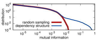
Figure 5: Non-null signatures of component dependency. The distribution of mutual information ($x$ axis), Eq. (29), for the random sampling protocol of Ref. Mazzolini et al. (2017) (thick red line) and for the model studied here (thin blue line). The frequency distribution of components was obtained by the positive model (with parameters $U=1000$, $D=1.5$, $k=50$), and $I(i,j)$ was computed for $R=1000$ realizations of both models. The distribution ($y$ axis) is the normalized empirical distribution for all realizations and all pairs $(i,j)$.

The model presented here provides the simplest generative mechanism producing collections of components consistent with a given dependency structure. Our construction extends the one proposed in Ref. Pang and Maslov (2013) to the case of components with non-binary abundance. While the distribution of component abundances has a power-law tail with an initial core, like in the case of Ref. Pang and Maslov (2013), the situation is more complex here, as the distribution of component abundances does not coincide with that of occurrences, due to the non-binary nature of the multiplicities. More general families of models can be defined by specifying the rules for selecting the abundance of nodes belonging to the dependency cones of more than one precursor. The additive choice taken here, where each cone determines the addition of one copy of each component belonging to it, provides a minimal model that is memoryless, and therefore still accessible analytically.

Since a wide variety of systems can be represented as collections of components belonging to a common pool, our model has general applicability. A special case is that of genomes, which deserves some observations. A dependency structure between genes represents the recipes binding the functional roles of different protein families, thereby determining their usefulness in the same genome. For example, a gene could depend on another if it is found downstream in the same metabolic pathway Pang and Maslov (2013). The topology of such dependency has not been fully characterized. Likely, it comprises both feedforward and feedback structures, as well as non-directed exclusion principles (whereby a gene might not be necessary or useful if another one is present). Concerning the additive choice discussed above, it is possible (and likely) that the choice of a memoryless process is too restrictive in the context of genomics. For instance, not all gene families required by the presence of multiple precursors need to be present in multiple copies. Future investigations could aim at defining more stringently from data the minimal features of a model of dependency that could realistically describe genomes. This could be inferred by the correlation structure of domain abundances from sets of entirely sequenced genomes.