Entanglement entropy in the Long-Range Kitaev chain

Abstract

In this paper we complete the study on the asymptotic behaviour of the entanglement entropy for Kitaev chains with long range pairing. We discover that when the couplings decay with the distance with a critical exponent new properties for the asymptotic growth of the entropy appear. The coefficient of the leading term is not universal any more and the connection with conformal field theories is lost. We perform a numerical and analytical approach to the problem showing a perfect agreement. In order to carry out the analytical study, a new technique for computing the asymptotic behaviour of block Toeplitz determinants with discontinuous symbols has been developed.

I Introduction

Entanglement plays a fundamental role in quantum phase transitions. In one dimensional critical theories with local interactions, the algebraic decay of the ground state correlation functions leads to the well-known logarithmic asymptotic growth of the entanglement entropy with a coefficient proportional to the central charge of the underlying conformal field theory Holzhey ; Latorre ; CarCal . On the other hand, outside criticality, the correlations decay exponentially and the entanglement entropy satisfies an area law Hastings ; Brandao .

The presence of long range interactions radically modifies the previous picture Cirac ; Koffel . As it is discussed in Vodola ; Vodola2 correlations can display exponential and algebraic decay even with non zero mass gap. This implies that the entanglement entropy may violate the area law while the system is non critical. This happens in the so-called Long-Range Kitaev chain Vodola ; Vodola2 , which has been the object of an intense study in the last years Regemortel ; Lepori ; Patrick ; Lepori2 ; Cirac2 . Apart from the theoretical interest, as a model to analyse the role of conformal symmetry in critical points, there has been recently a spectacular development of experimental devices where these long range interactions can be simulated Micheli ; Islam ; Britton ; Richerme ; Labuhn .

In Ares3 we studied the behaviour of the entanglement entropy of the vacuum with the size of the subsystem for a Long-Range Kitaev chain. In order to compute the asymptotic behaviour of the entropy we had to establish new results on block Toeplitz determinants with discontinuous symbol. In that paper we obtained two different regimes depending on the exponent $\zeta$ that governs the decay of the couplings. The two regimes were already analysed numerically in Vodola and correspond respectively to $\zeta>1$ and $\zeta<1$. In this paper we study the intermediate critical case $\zeta=1$ for which new physical properties for the entropy show themselves. From the point of view of Toeplitz determinants, the critical exponent posses new challenges that must be solved before being able to determine the asymptotic behaviour of the entanglement entropy. This task is carried out in the rest of the paper.

II The model

The Long-Range Kitaev chain is a unidimensional homogeneous fermionic chain with nearest-neighbour hopping and power-like decaying pairings,

$$H=\sum_{n=1}^{N}\Big{(}a_{n}^{\dagger}a_{n+1}+a_{n+1}^{\dagger}a_{n}+h\,a_{n}^{\dagger}a_{n}+\sum_{|l|<N/2}\frac{l}{|l|^{\zeta+1}}(a_{n}^{\dagger}a_{n+l}^{\dagger}-a_{n}a_{n+l})\Big{)}-\frac{Nh}{2},$$ (1)

where $a_{n}^{\dagger}$, $a_{n}$ are fermionic creation and annihilation operators acting on the site $n$, satisfying the canonical anticommutation relations $\{a_{n},a_{m}^{\dagger}\}=\delta_{nm}$, $\{a_{n}^{\dagger},a_{m}^{\dagger}\}=\{a_{n},a_{m}\}=0$ and periodic boundary conditions, that is $a_{n+N}=a_{n}$.

The exponent $\zeta>0$ characterises the dumping of the coupling with the distance. Its value plays a decisive role in the growth rate of the Rényi entanglement entropy Vodola ; Ares3 ; Vodola2 . In a previous work Ares3 we analytically studied the leading asymptotic behaviour with the size of an interval of the chain $|X|$ when $\zeta\neq 1$. There we found that the entanglement entropy $S_{\alpha,X}$ behaves as

$$S_{\alpha,X}=\frac{\alpha+1}{6\alpha}c\log|X|+\dots$$ (2)

up to finite contributions in the large $|X|$ limit, with an effective central charge $c$ given by

$$c=\begin{cases}0&\zeta>1\ {\rm and}\ h\not=\pm 2,\cr 1/2&\zeta>1\ {\rm and}\ h=\pm 2\ \ {\rm or}\ \ \zeta<1\ {\rm and}\ h\not=2,\cr 1&\zeta<1\ {\rm and}\ h=2.\end{cases}$$ (3)

This is in agreement with the numerical studies previously performed in Vodola .

We see that the case $\zeta=1$ is the only one not covered in the previous expression. To our knowledge this case has not been considered in the literature in spite of its physical interest as it may be experimentally implemented with chains of magnetic impurities on an s-wave superconductor Pientka . Our reason to exclude this value in Ares3 is that in order to address this case we required a technical result that was not available at the moment we wrote the previous paper. In this paper we fill this gap and obtain the scaling behaviour in the most general situation. We find that along the line $\zeta=1$ the entanglement entropy grows logarithmically but with a proportionality constant that can not be expressed in terms of an effective central charge. In the following we will develop the technical tools required for the previous computation.

We must first solve the model in (1). Since it is a translational invariant and quadratic Hamiltonian, one can diagonalise it performing a Fourier plus a Bogoliubov transformation (see e.g. Ref. Ares3 ). After the latter, the Hamiltonian reads

$$H=\sum_{k=0}^{N-1}\Lambda_{k}d_{k}^{\dagger}d_{k},$$

where $d_{k}$ and $d_{k}^{\dagger}$ are also fermionic operators and $\Lambda_{k}$ is the dispersion relation

$$\Lambda_{k}=\sqrt{(h+2\cos\theta_{k})^{2}+4\left(\sum_{l=1}^{N/2}\sin(l\theta_{k})l^{-\zeta}\right)^{2}},\quad\theta_{k}=\frac{2\pi k}{N}.$$

If we take now the thermodynamic limit $N\to\infty$, $\theta_{k}$ is replaced by a continuous variable $\theta\in[-\pi,\pi)$ and the dispersion relation can be expressed as

$$\Lambda(\theta)=\sqrt{(h+2\cos\theta)^{2}+|G_{\zeta}(\theta)|^{2}},$$ (4)

where $G_{\zeta}(\theta)\equiv\Xi_{\zeta}({\rm e}^{{{\rm i}}\theta})$ and

$$\Xi_{\zeta}(z)=\sum_{l=1}^{\infty}({z^{l}-z^{-l}})~{}l^{-\zeta}={\rm Li}_{\zeta}(z)-{\rm Li}_{\zeta}(z^{-1}).$$

The function ${\rm Li}_{\zeta}$ stands for the polylogarithm of order $\zeta$. This is a multivalued function, analytic outside the real interval $[1,\infty)$ and has a finite limit at $z=1$ for $\zeta>1$ while it diverges at that point for $\zeta<1$. For $\zeta=1$ the polylogarithm function reduces to the logarithm ${\rm Li}_{1}(z)=-\log(1-z)$. We shall take as its branch cut the real interval $[1,\infty)$, thus $\Xi_{1}(z)$ has a branch cut along $[0,\infty)$. These properties will be crucial in the study of the entanglement entropy of the ground state of (1).

Since $\Lambda_{k}\geq 0$, the state of minimum energy $\mathinner{|{{\rm GS}}\rangle}$ is the Fock space vacuum for the Bogoliubov modes, i. e. $d_{k}\mathinner{|{\mathrm{GS}}\rangle}=0$ for all $k$. If we split the system in two subchains $X$, $Y$ of contiguous sites, the Hilbert space factorises $\mathcal{H}=\mathcal{H}_{X}\otimes\mathcal{H}_{Y}$. Then the Rényi entanglement entropy of $\mathinner{|{{\rm GS}}\rangle}$ is defined as

$$S_{\alpha,X}=\frac{1}{1-\alpha}\log\mathop{\mbox{Tr}}\nolimits(\rho_{X}^{\alpha}),$$

with $\rho_{X}=\mathop{\mbox{Tr}}\nolimits_{\mathcal{H}_{Y}}\mathinner{|{{\rm GS}}\rangle}\mathinner{\langle{{\rm GS}}|}$ the reduced density matrix of $X$. As it is well known, for Gaussian theories where the Wick theorem is satisfied, as it is our case, the entanglement entropy of this state can be computed from the correlation matrix Sorkin ; Latorre ; Peschel . In fact Jin ; Its ; Its2 ,

$$S_{\alpha,X}=\lim_{\delta\to 1^{+}}\frac{1}{4\pi{{\rm i}}}\oint_{C}f_{\alpha}(\lambda/\delta)\frac{{\rm d}}{{\rm d}\lambda}\log D_{X}(\lambda){\rm d}\lambda,$$ (5)

where

$$f_{\alpha}(x)=\frac{1}{1-\alpha}\log\left[\left(\frac{1+x}{2}\right)^{\alpha}+\left(\frac{1-x}{2}\right)^{\alpha}\right],$$ (6)

and $D_{X}(\lambda)=\det(\lambda I-V_{X})$ with $V_{X}$ the restriction of the ground state correlation matrix to the sites that belong to the subsystem $X$,

$$(V_{X})_{nm}=\left\langle\left(\begin{array}[]{c}a_{n}\\ a_{n}^{\dagger}\end{array}\right)\left(a_{m},a_{m}^{\dagger}\right)\right\rangle-\delta_{nm}I,\quad n,m\in X.$$

The integration contour and the branch choice for $f_{\alpha}(\lambda/\delta)$ are represented in the Fig. 1.

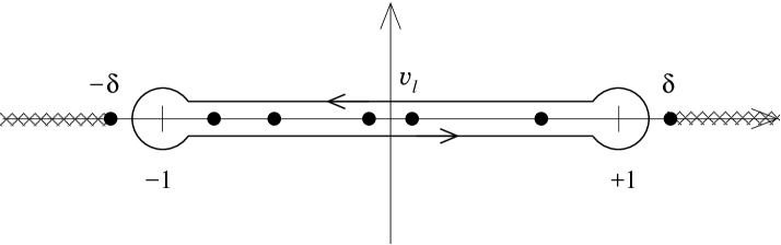
Figure 1: Contour of integration, cuts and poles for the computation of $S_{\alpha,X}$. The contour surrounds the eigenvalues $v_{l}$ of $V_{X}$, all of them lying on the real interval $[-1,1]$. The cuts for the function $f_{\alpha}$ extend to $\pm\infty$.

Due to the translational invariance of the Hamiltonian and given the choice of the subsystem $X$, which is composed of contiguous sites, the correlation matrix is a block Toeplitz matrix,

$$(V_{X})_{nm}=\frac{1}{2\pi}\int_{-\pi}^{\pi}\mathcal{{G}}(\theta){\rm e}^{{{\rm i}}\theta(n-m)}{\rm d}\theta,$$ (7)

generated by a 2-dimensional symbol $\mathcal{{G}}(\theta)$ which, for the ground state of the Hamiltonian (1), has the form

$$\mathcal{{G}}(\theta)=\frac{1}{\Lambda(\theta)}\left(\begin{array}[]{cc}h+2\cos\theta&G_{\zeta}(\theta)\\ -G_{\zeta}(\theta)&-h-2\cos\theta\end{array}\right).$$ (8)

By virtue of (5), the asymptotic behaviour of $S_{\alpha,X}$ can be obtained from that of the determinant $D_{X}(\lambda)$. The discontinuities of the symbol (8) will give the leading dominant term. In Ares3 , we already computed them for $\zeta\neq 1$, where the lateral limits of each discontinuity commute. For $\zeta=1$ the symbol has a non-commuting discontinuity and we lacked a way to determine its contribution. In the following we shall solve this problem.

III Determinant of block Toeplitz matrices with discontinuous symbol

In this section we shall study the scaling properties of the determinant of a block Toeplitz matrix with piecewise continuous matrix valued symbol.

Given a $d\times d$ dimensional matrix valued function $\mathcal{M}(\theta)$ we shall denote by $T_{X}[\mathcal{M}]$ its associated $|X|\!\cdot\!d$ dimensional block Toeplitz matrix, i.e. for every $k,l=1,\dots,|X|$ there is a $d\times d$ block given by

$$\big{(}T_{X}[\mathcal{M}]\big{)}_{k,l}=\frac{1}{2\pi}\int_{-\pi}^{\pi}\mathcal{M}(\theta){\rm e}^{{\rm i}\theta(k-l)}{\rm d}\theta.$$

We shall denote by $D_{X}[\mathcal{M}]=\det T_{X}[\mathcal{M}]$.

From Szego-Widom theorem Widom ; Widom2 ; Widom3 we know that the leading linear term of $\log D_{X}[\mathcal{M}]$ is given by

$$\log D_{X}[\mathcal{M}]=\frac{|X|}{2\pi}\int_{-\pi}^{\pi}\log\det\mathcal{M}(\theta){\rm d}\theta+\cdots,$$

where we assume $\det\mathcal{M}(\theta)\not=0$ and the dots denote subdominant contributions in the limit $|X|\to\infty$.

As it is discussed in Ares3 , the next subdominant contribution for a piecewise continuous symbol with jump discontinuities at $\theta_{r}$, for $r=1,\dots,R$, is logarithmic in $|X|$ and has the form

$$\log D_{X}[\mathcal{M}]=\frac{|X|}{2\pi}\int_{-\pi}^{\pi}\log\det\mathcal{M}(\theta){\rm d}\theta+\log|X|\sum_{r=1}^{R}b_{r}+\cdots,$$ (9)

where the coefficient $b_{r}$ depends uniquely on the lateral limits at the discontinuity $\theta_{r}$.

In the particular case in which the two lateral limits commute an explicit expression for $b_{r}$ is proposed in Ares3 . We review here this result.

If for a discontinuity $\theta_{r}$ the two lateral limits

$$\mathcal{M}_{r}^{-}=\lim_{\theta\to\theta_{r}^{-}}\mathcal{M}(\theta)\qquad{\rm and}\qquad\mathcal{M}_{r}^{+}=\lim_{\theta\to\theta_{r}^{+}}\mathcal{M}(\theta)$$

commute and are diagonalisable, then we can diagonalise both in the same basis. Let us denote by $\mu_{r,j}^{\pm},\ j=1,\dots,d$ the corresponding eigenvalues for each lateral limit of the discontinuity at $\theta_{r}$. Then inspired by the similar case for a scalar symbol Fisher ; BasorMorrison , we conjectured in Ares3 that the logarithmic coefficients are given by

$$b_{r}=\frac{1}{4\pi^{2}}\sum_{j=1}^{d}\left(\log\frac{\mu_{r,j}^{-}}{\mu_{r,j}^{+}}\right)^{2}.$$ (10)

This conjecture was verified numerically to all attainable precision. Note that the previous expression can be written in the more compact (and meaningful) form

$$b_{r}=\frac{1}{4\pi^{2}}\mathop{\mbox{Tr}}\nolimits\left[\log\mathcal{M}_{r}^{-}(\mathcal{M}_{r}^{+})^{-1}\right]^{2}.$$ (11)

In the following we shall argue that if this result is true, it is also valid when the two lateral limits do not commute.

In order to show it, we have to invoke an old result by Widom Widom2 that, in the particular case that concerns our derivation, can be stated in the very simple form:

For any $d\times d$ constant matrix $\mathcal{C}$ and any symbol $\mathcal{M}(\theta)$ as before we have

$$T_{X}[\mathcal{M}\mathcal{C}]=T_{X}[\mathcal{M}]T_{X}[\mathcal{C}].$$

Actually $T_{X}[\mathcal{C}]=I_{|X|}\otimes\;\mathcal{C}$ and the relation above immediately follows. For the determinants we have

$$\log D_{X}[\mathcal{M}\mathcal{C}]=\log D_{X}[\mathcal{M}]+|X|\log\det\mathcal{C}.$$

Now, in the general case of a piecewise continuous symbol with non commuting lateral limits, $\mathcal{M}_{r}^{\pm}$, at the discontinuity point $\theta_{r}$, we can apply the previous result choosing the constant symbol $\mathcal{C}=(\mathcal{M}_{r}^{+})^{-1}$. Hence we have

$$\log D_{X}[\mathcal{M}]=\log D_{X}[\mathcal{M}(\mathcal{M}_{r}^{+})^{-1}]+|X|\log\det\mathcal{M}_{r}^{+}.$$ (12)

Now, applying the expansion in (9) to the new symbol $\mathcal{M}(\mathcal{M}_{r}^{+})^{-1}$ we have

$$\log D_{X}[\mathcal{M}(\mathcal{M}_{r}^{+})^{-1}]=\frac{|X|}{2\pi}\int_{-\pi}^{\pi}\log\det\mathcal{M}(\theta){\rm d}\theta-|X|\log\det\mathcal{M}_{r}^{+}+\log|X|\sum_{r=1}^{R}b^{\prime}_{r}+\cdots.$$ (13)

But the two lateral limits at $\theta_{r}$ are $\mathcal{M}_{r}^{-}(\mathcal{M}_{r}^{+})^{-1}$ and $I$ which, of course, commute. Therefore, we can apply the previous result on commuting lateral symbols and we obtain

$$b^{\prime}_{r}=\frac{1}{4\pi^{2}}\mathop{\mbox{Tr}}\nolimits\left[\log\mathcal{M}_{r}^{-}(\mathcal{M}_{r}^{+})^{-1}\right]^{2}.$$

If we combine (9), (12) and (13) we get $b_{r}=b^{\prime}_{r}$ and therefore (11) is valid even if the lateral limits do not commute, as stated.

IV Entanglement entropy

After the technical parenthesis of the previous section we continue with the main goal of the paper. Our task is to obtain the scaling behaviour of the entanglement entropy $S_{\alpha,X}$ as derived from formula (5).

For that purpose we must use the results of the previous section to compute the block Toeplitz determinant $D_{X}(\lambda)$ or, equivalently, $D_{X}[\mathcal{G}_{\lambda}]$ in the notation of the last section. Here we have introduced the 2-dimensional symbol $\mathcal{G}_{\lambda}(\theta)=\lambda I-\mathcal{G}(\theta)$ with $\mathcal{G}(\theta)$ taken from (8).

The linear term of $\log D_{X}(\lambda)$ is derived from the Szego estimate and, given that $\det\mathcal{G}_{\lambda}(\theta)=\lambda^{2}-1$, the asymptotic behaviour is

$$\log D_{X}(\lambda)=|X|\log(\lambda^{2}-1)+\log|X|\sum_{r}b_{r}(\lambda)+\dots,$$

where as before the dots represent finite terms in the large $|X|$ limit and the coefficients of the logarithmic piece are associated to the discontinuities of $\mathcal{G}_{\lambda}$ by the expression derived in the previous section. Namely, the coefficient $b_{r}(\lambda)$ associated to the discontinuity at $\theta_{r}$ is given by

$$b_{r}(\lambda)=\frac{1}{4\pi^{2}}\mathop{\mbox{Tr}}\nolimits\left[\log\mathcal{G}_{\lambda,r}^{-}(\mathcal{G}_{\lambda,r}^{+})^{-1}\right]^{2}.$$

Therefore, to proceed we must identify the location of the jumps of $\mathcal{G}_{\lambda}$ and compute the lateral limits.

It is clear that the possible sources of discontinuities for $\mathcal{G}_{\lambda}$ are the discontinuities or the zeros of $\Lambda(\theta)$. In our case of interest, $\zeta=1$, these are $\theta=0$, for which

$$G_{\zeta=1}(\theta)={\rm i}(\pi-\theta),\ \ \theta\in[0,2\pi)$$

has a jump; and, for $h=2$, $\theta=\pi$ where $\Lambda(\theta)$ vanishes. We will discuss separately both discontinuity points.

Let us call $b_{0}$ the coefficient in the expansion of $\log D_{X}(\lambda)$ associated to $\theta=0$. The two lateral limits are conveniently expressed in terms of the Pauli sigma matrices

$$\mathcal{G}_{\lambda,0}^{\pm}=\lambda I-\cos\xi\ \sigma_{z}\pm\sin\xi\ \sigma_{y},$$

where

$$\cos\xi=\frac{h+2}{\sqrt{(h+2)^{2}+\pi^{2}}},\quad\sin\xi=\frac{\pi}{\sqrt{(h+2)^{2}+\pi^{2}}}.$$

Clearly for $\xi\not=\pi/2$ the two limits do not commute and we are bound to use the results of the previous section.

With a little algebra we get

$$\mathcal{G}_{\lambda,0}^{-}(\mathcal{G}_{\lambda,0}^{+})^{-1}=\frac{1}{\lambda^{2}-1}\left((\lambda^{2}-\cos 2\xi)I-2\lambda\sin\xi\ \sigma_{y}-{\rm i}\sin\xi\ \sigma_{x}\right).$$

In order to compute $b_{0}(\lambda)$ we need the eigenvalues $\mu_{\pm}(\lambda)$ of the previous matrix. They can be written

$$\mu_{\pm}(\lambda)=\left(\frac{\sqrt{\lambda^{2}-\cos^{2}\xi}\pm\sin\xi}{\sqrt{\lambda^{2}-1}}\right)^{2}.$$

Notice also that we have

$$\mu_{+}(\lambda)=\mu_{-}(\lambda)^{-1}.$$

Putting everything together we finally obtain

$$b_{0}(\lambda) = \frac{1}{4\pi^{2}}\left[\left(\log\mu_{+}(\lambda)\,\right)^{2}+\left(\log\mu_{-}(\lambda)\,\right)^{2}\right]$$ (14)

$$= \frac{2}{\pi^{2}}\left(\log\frac{\sqrt{\lambda^{2}-\cos^{2}\xi}+\sin\xi}{\sqrt{\lambda^{2}-1}}\right)^{2}.$$ (15)

As we discussed before, for $h\not=2$ this is the only discontinuity of the symbol and therefore the only contribution to the logarithmic term for $\log D_{X}(\lambda)$. Namely

$$\log D_{X}(\lambda)=|X|\log(\lambda^{2}-1)+\log|X|b_{0}(\lambda)+\dots.$$

This must be inserted into (5) to derive the scaling behaviour of the entanglement entropy.

The linear term is obtained from the integral

$$\lim_{\delta\to 1^{+}}\frac{1}{2\pi{{\rm i}}}\oint_{C}f_{\alpha}(\lambda/\delta)\frac{{\lambda}}{\lambda^{2}-1}{\rm d}\lambda=\frac{1}{2}(f_{\alpha}(1)+f_{\alpha}(-1))=0,$$

where the Cauchy’s residue theorem has been used and from the expression in (6) we immediately see that $f_{\alpha}(\pm 1)=0$.

The previous result: vanishing of the term that scales linearly with the size of the subsystem, is in agreement with the area law, that states that in the ground state of a local theory the entanglement entropy is not an extensive quantity. As we will see now the area law has corrections and the entanglement entropy scales with the logarithm of the size of the subsystem rather than going to a constant.

The coefficient of the logarithmic term for the entropy, that we denote by $B_{\alpha}$, gets just one contribution, named $B_{\alpha,0}$, from the discontinuity at $\theta=0$; we are considering $h\not=2$. It can be computed from (5)

$$B_{\alpha,0} = \lim_{\delta\to 1^{+}}\frac{1}{4\pi{{\rm i}}}\oint_{C}f_{\alpha}(\lambda/\delta)\frac{{\rm d}b_{0}(\lambda)}{{\rm d}\lambda}{\rm d}\lambda$$ (16)

$$= -\lim_{\delta\to 1^{+}}\frac{1}{2\pi^{3}{{\rm i}}}\oint_{C}\frac{{\rm d}f_{\alpha}(\lambda/\delta)}{{\rm d}\lambda}\left(\log\frac{\sqrt{\lambda^{2}-\cos^{2}\xi}+\sin\xi}{\sqrt{\lambda^{2}-1}}\right)^{2}{\rm d}\lambda,$$ (17)

where, for convenience, we have performed an integration by parts. The branch cuts of the different multivalued functions involved in the integral are depicted in the Fig. 2.

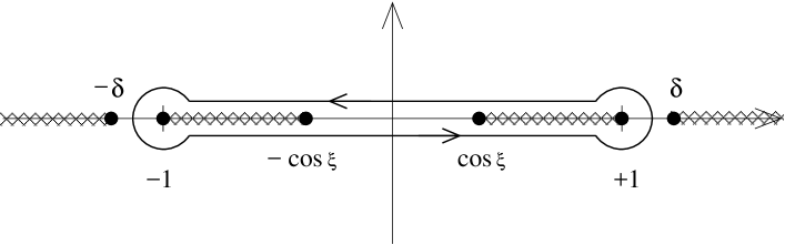
Figure 2: Contour of integration and cuts of the integrand in (16) for the computation of $B_{\alpha,0}$. The cuts from $\pm\delta$ to the infinity correspond to ${\rm d}f_{\alpha}(\lambda/\delta)/{\rm d}\lambda$ while the cuts inside the contour, $[-1,-\cos\xi]$ and $[\cos\xi,1]$, are due to the other factor of the integrand.

Now it is possible to take the limit in (16) and, given that $f_{\alpha}$ is an even function, the complex integral can be reduced to the following real one

$$B_{\alpha,0}=\frac{2}{\pi^{2}}\int_{\cos\xi}^{1}\frac{{\rm d}f_{\alpha}(\lambda)}{{\rm d}\lambda}\log\frac{\sqrt{1-\lambda^{2}}}{\sqrt{\lambda^{2}-\cos^{2}\xi}+\sin\xi}{\rm d}\lambda,$$ (18)

where we take positive square roots.

Note that for integer $\alpha>1$

$$\frac{{\rm d}f_{\alpha}(\lambda)}{{\rm d}\lambda}=\frac{\alpha}{1-\alpha}\frac{(1+\lambda)^{\alpha-1}-(1-\lambda)^{\alpha-1}}{(1+\lambda)^{\alpha}+(1-\lambda)^{\alpha}},$$ (19)

is a meromorphic function with poles along the imaginary axis located at

$$\lambda_{k}={{\rm i}}\tan\frac{\pi(2k-1)}{2\alpha},\quad k=1,2,\dots,\alpha,\ {\rm with}\ k\not=\frac{\alpha+1}{2}.$$

Hence, by sending the integration contour in (16) to infinity we can reduce the integral to the computation of the corresponding residues. In this way we get a completely explicit expression for $B_{\alpha,0}$ (valid only for integer $\alpha>1$)

$$B_{\alpha,0}=\frac{1}{\pi^{2}(\alpha-1)}\sum_{k=1}^{\alpha}\arctan^{2}\frac{\sin\xi}{\sqrt{\cos^{2}\xi+|\lambda_{k}|^{2}}}.$$

In particular, for $\alpha=2,3$ the sum in the previous expression reduces to

$$B_{2,0} = \frac{2}{\pi^{2}}\arctan^{2}\frac{\sin\xi}{\sqrt{\cos^{2}\xi+1}},$$

$$B_{3,0} = \frac{1}{\pi^{2}}\arctan^{2}\frac{\sin\xi}{\sqrt{\cos^{2}\xi+1/3}}.$$

In the Fig. 3 we numerically check the scaling of the entanglement entropy given by the expression (18) that we have just obtained for the logarithmic coefficient $B_{\alpha}$. Although we have only plotted the von Neumann entropy, we have seen that the agreement with the numerical computations is just as good for other values of $\alpha$.

Figure 3: Numerical check of the asymptotic scaling of the von Neumann entanglement entropy ($\alpha=1$) with the length of the interval $|X|$ for $\zeta=1$ and different values of $h$. The dots represent the numerical computation while the solid lines correspond to the curve $B_{1}\log|X|+{\rm constant}$ where $B_{1}=B_{1,0}$ for $h\neq 2$ and $B_{1}=B_{1,0}+1/6$ if $h=2$. $B_{1,0}$ is given by (18). The constant is obtained by fitting the numerical and the analytical results at $|X|=1000$.

For local theories it is possible to relate the entanglement entropy to universal properties of conformal field theories. In this case the coefficient of the logarithmic term in the expansion should read

$$B_{\alpha}=\frac{\alpha+1}{6\alpha}c,$$ (20)

where $c$, the central charge, is a constant that depends on the universality class of the underlying conformal field theory. In particular this relation implies

$$B_{2}=\frac{9}{8}B_{3},$$

something that, for general $h$, does not hold in our case. The reason for that could be that couplings in our theory have infinite range and therefore it cannot be related to any local field theory. However, as it was shown in Ares3 , when the coupling constants decay faster ($\zeta>1$) or slower ($\zeta<1$) than our critical case, relation (20) also holds, even if the theory is not local. Another instance in which $(\ref{central_charge})$ holds is when $h=-2$, then $\xi=\pi/2$ and we have

$$B_{2,0}=\frac{1}{8},\qquad B_{3,0}=\frac{1}{9},$$

which fulfil (20) with $c=1/2$.

This is the whole story about the logarithmic coefficient, and $B_{\alpha}=B_{\alpha,0}$ for $h\not=2$, as we discussed before. However for $h=2$ the dispersion relation $\Lambda(\theta)$ vanishes at $\theta=\pi$ and it induces a discontinuity in the symbol. The two lateral limits are

$$\mathcal{G}_{\lambda,\pi}^{\pm}=\lambda I\pm\sigma_{y}$$

and its contribution to the logarithmic term in the expansion of $\log D_{X}(\lambda)$ is given by

$$b_{\pi}(\lambda) = \frac{1}{4\pi^{2}}\mathop{\mbox{Tr}}\nolimits\left[\log\mathcal{G}_{\lambda,\pi}^{-}(\mathcal{G}_{\lambda,\pi}^{+})^{-1}\right]^{2}$$ (21)

$$= \frac{1}{2\pi^{2}}\left(\log\frac{\lambda+1}{\lambda-1}\right)^{2}.$$ (22)

Associated to that there is a new logarithmic term for the entropy whose coefficient is given by

$$B_{\alpha,\pi}=\lim_{\delta\to 1^{+}}\frac{1}{4\pi{{\rm i}}}\oint_{C}f_{\alpha}(\lambda/\delta)\frac{{\rm d}}{{\rm d}\lambda}b_{{\pi}}(\lambda){\rm d}\lambda=\frac{\alpha+1}{12\alpha}.$$ (23)

In the light of the previous discussion this contribution to the logarithmic term can be interpreted as coming from a conformal field theory with central charge $c=1/2$.

We would like to stress again that the last interpretation is valid only for part of the contribution to the logarithmic term of the entropy. One should consider the whole coefficient $B_{\alpha}=B_{\alpha,0}+B_{\alpha,\pi}$, that includes the discontinuity at $\theta=0$, and this, for $h=2$, does not behave as predicted by the conformal field theory under variations of $\alpha$. Observe that in the Fig. 3 we have considered this particular point. Also in this case the analytical formulae we have obtained are in agreement with the numerical results.

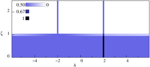
Figure 4: Plot of the different regions in the $(h,\zeta)$ plane according to the coefficient $B_{2}$ of the logarithmic scaling for the entanglement entropy. The colouring stands for the value of $2B_{2}$: from white for $B_{2}=0$ to black when $B_{2}=1/2$.

As a summary, in the Fig. 4 we have recollected the previous known results (2), (3) outside the line $\zeta=1$ together with those obtained in this section for $\zeta=1$. We have coloured the parameter space $(h,\zeta)$ according to the value of the logarithmic term $B_{\alpha}$. The model is critical, the mass gap is zero, only in the lines $h=\pm 2$. Note, however, that the entanglement entropy scales logarithmically for $\zeta\leq 1$ even outside criticality.

As a further check of the results obtained in the previous section we shall consider a variant of the Long-Range Kitaev Chain. Namely we shall discuss the case in which we have two singularities in the symbol (instead of one) located at $\theta=\pm\phi$. One reason for this is connected to the study of the Möbius symmetry introduced in Ares2 ; Ares4 . While $\theta=0$ is a fixed point of the above mentioned transformations $\theta=\pm\phi$ is not, which enriches the symmetry. We do not pursue the analysis of Möbius transformations in this paper.

The new singularities in the symbol can be obtained by adding to (1) an oscillatory factor in the pairing,

$$H^{\prime}=\sum_{n=1}^{N}\Big{(}a_{n}^{\dagger}a_{n+1}+a_{n+1}^{\dagger}a_{n}+h\,a_{n}^{\dagger}a_{n}+\sum_{|l|<N/2}\frac{l\cos(l\phi)}{|l|^{\zeta+1}}(a_{n}^{\dagger}a_{n+l}^{\dagger}-a_{n}a_{n+l})\Big{)}-\frac{Nh}{2},$$ (24)

with $\phi\in[0,\pi)$.

In the thermodynamic limit $N\to\infty$, the dispersion relation is

$$\Lambda^{\prime}(\theta)=\sqrt{(h+2\cos\theta)^{2}+|G_{\zeta,\phi}(\theta)|^{2}},$$

where $G_{\zeta,\phi}(\theta)=\Xi_{\zeta,\phi}({\rm e}^{{{\rm i}}\theta})$, and

$$G_{\zeta,\phi}(\theta) = \sum_{l=1}^{\infty}\frac{\cos(l\phi)}{l^{\zeta}}({\rm e}^{{{\rm i}}\,\theta l}-{\rm e}^{-{{\rm i}}\,\theta l})$$

$$= \frac{1}{2}\left[{\rm Li}_{\zeta}({\rm e}^{{{\rm i}}(\phi+\theta)})-{\rm Li}_{\zeta}({\rm e}^{{{\rm i}}(\phi-\theta)})+{\rm Li}_{\zeta}({\rm e}^{-{{\rm i}}(\phi-\theta)})-{\rm Li}_{\zeta}({\rm e}^{-{{\rm i}}(\phi+\theta)})\right].$$

This function vanishes at $\theta=0$ and $\pi$, it is smooth for $\zeta>1$, diverges at $\theta=\pm\phi$ for $\zeta<1$ and for our particular case of interest in this paper, $\zeta=1$, it reads

$$G_{1,\phi}(\theta)=\left\{\begin{array}[]{cc}-{{\rm i}}(\pi+\theta),&-\pi\leq\theta\leq-\phi,\\ -{{\rm i}}\theta,&-\phi<\theta<\phi,\\ {{\rm i}}(\pi-\theta),&\phi\leq\theta<\pi.\end{array}\right.$$

It has a jump at $\theta=\phi$ with lateral limits ${\rm i}\phi$ and ${\rm i}(\pi-\phi)$ and another one at $\theta=-\phi$ with limits ${\rm i}(\phi-\pi)$ and $-{\rm i}\phi$.

The symbol of the correlation matrix can be written

$$\mathcal{{G}}^{\prime}(\theta)=\frac{1}{\Lambda^{\prime}(\theta)}\left(\begin{array}[]{cc}h+2\cos\theta&G_{\zeta,\phi}(\theta)\\ -G_{\zeta,\phi}(\theta)&-h-2\cos\theta\end{array}\right).$$

For $h\not=\pm 2$ and $\zeta=1$ the only jumps of $\mathcal{G}_{\lambda}^{\prime}(\theta)=\lambda I-\mathcal{{G}}^{\prime}(\theta)$ take place at $\theta=\pm\phi$. We shall compute separately the contribution of each discontinuity to the coefficient of the logarithmic term in the expansion of the entanglement entropy.

In first place we consider the point $\theta=\phi$. The lateral limits of $\mathcal{G}_{\lambda}^{\prime}(\theta)$ are

$$\mathcal{G}_{\lambda,\phi}^{\prime\pm}=\lambda I-\cos\xi^{\pm}\;\sigma_{z}-\sin\xi^{\pm}\,\sigma_{y},$$

where

$$\cos\xi^{+}=\frac{h+2\cos\phi}{\sqrt{(h+2\cos\phi)^{2}+(\phi-\pi)^{2}}},\quad\sin\xi^{+}=\frac{\phi-\pi}{\sqrt{(h+2\cos\phi)^{2}+(\phi-\pi)^{2}}}$$

and

$$\cos\xi^{-}=\frac{h+2\cos\phi}{\sqrt{(h+2\cos\phi)^{2}+\phi^{2}}},\quad\quad\quad\ \sin\xi^{-}=\frac{\phi}{\sqrt{(h+2\cos\phi)^{2}+\phi^{2}}}.\quad\quad\$$

The eigenvalues of $\mathcal{G}_{\lambda,\phi}^{\prime-}(\mathcal{G}_{\lambda,\phi}^{\prime+})^{-1}$ are:

$$\mu^{\prime}_{\pm}(\lambda)=\left(\frac{\sqrt{\lambda^{2}-\cos^{2}(\Delta\xi/2)}\pm\sin(\Delta\xi/2)}{\sqrt{\lambda^{2}-1}}\right)^{2},$$

where $\Delta\xi=\xi^{+}-\xi^{-}$.

Observe that the expression for the eigenvalues is exactly that of the model in the previous section, with the only change of $\xi$ by $\Delta\xi/2$.

Therefore the contribution of this discontinuity to the logarithmic coefficient of the entanglement entropy, $B^{\prime}_{\alpha,\phi}$, can be written

$$B^{\prime}_{\alpha,\phi}=\frac{2}{\pi^{2}}\int_{\cos\frac{\Delta\xi}{2}}^{1}\frac{{\rm d}f_{\alpha}(\lambda)}{{\rm d}\lambda}\log\frac{\sqrt{1-\lambda^{2}}}{\sqrt{\lambda^{2}-\cos^{2}(\Delta\xi/2)}+\sin(\Delta\xi/2)}{\rm d}\lambda,$$ (25)

and the corresponding integrated expression for integer $\alpha>1$

$$B^{\prime}_{\alpha,\phi}=\frac{1}{\pi^{2}(\alpha-1)}\sum_{k=1}^{\alpha}\arctan^{2}\frac{\sin(\Delta\xi/2)}{\sqrt{\cos^{2}(\Delta\xi/2)+|\lambda_{k}|^{2}}}.$$ (26)

The other discontinuity point, $\theta=-\phi$, can be computed along the same lines. Actually the only difference with respect to the previous case is that we have to replace $\xi^{+}$ and $\xi^{-}$ with $-\xi^{-}$ and $-\xi^{+}$ respectively. Hence, $\Delta\xi$ is unchanged, $B^{\prime}_{\alpha,-\phi}=B^{\prime}_{\alpha,\phi}$ and for $h\not=\pm 2$ the asymptotic behaviour of the entanglement entropy for this modified Long-Range Kitaev chain is

$$S^{\prime}_{\alpha,X}=2B^{\prime}_{\alpha,\phi}\log|X|+\dots,$$

with $B^{\prime}_{\alpha,\phi}$ given above. In the Fig. 5 we compare the numerical value of the entanglement entropy for different values of $h$ along the line $\zeta=1$ when $\alpha=2$ and $\phi=\pi/4$. The agreement between them makes us conclude that the expression that we have obtained for the leading contribution of the discontinuities of a block Toeplitz matrix is correct.

Figure 5: Rényi entanglement entropy with $\alpha=2$ as a function of the length $|X|$ of the interval for $\phi=\pi/4$, $\zeta=1$ and different values of $h$. The dots correspond to the numerical entropy while the solid lines are our analytical prediction $B^{\prime}_{2}\log|X|+{\rm constant}$ with $B^{\prime}_{2}$ that obtained in the text: $B^{\prime}_{2}=2B^{\prime}_{2,\pi/4}+1/4$ for $h=\pm 2$ and $B^{\prime}_{2}=2B^{\prime}_{2,\pi/4}$ with $B_{2,\pi/4}$ given by (26). The constant is obtained by fitting the numerical and the analytical results at $|X|=1000$.

For completeness we also consider the case $h=\pm 2$ that was excluded in the previous considerations. The Hamiltonian in this case is gap-less and the coefficient in the expansion of the entanglement entropy gets an extra coefficient due to this fact. In both cases $h=2$ or $-2$ the extra term is the same and coincides with the one we obtained in the previous section. Namely, for $h=\pm 2$ we have

$$B_{\alpha}^{\prime}=2B^{\prime}_{\alpha,\phi}+\frac{\alpha+1}{12\alpha}.$$

In the Fig. 5 we also checked the case $h=2$ when $\alpha=2$. Observe that the numerical values agree with the form of $B^{\prime}_{\alpha}$ deduced for this case.

V Conclusions

In this work, we have completed the study of the scaling behaviour of the ground state entanglement entropy in the Long-Range Kitaev chain that we started in Ares3 . Our analysis is based on the relation between the entanglement entropy and the determinant of the correlation matrix. Since the chain is translational invariant, the correlation matrix for a single interval is block Toeplitz.

If the symbol of the block Toeplitz matrix is continuous, the entropy scales with the area of the subsystem and hence has a finite asymptotic limit. On the contrary, the presence of discontinuities gives rise to corrections to the area law, leading to a logarithmic growth of the entropy with the size of the interval. In Ares3 we considered the case $\zeta\neq 1$. There, we were able to compute the asymptotic behaviour of the entanglement entropy thanks to the fact that the lateral limits of the jump discontinuities commute in that case. However, for the intermediate value $\zeta=1$ we have jump discontinuities whose lateral limits do not commute and the results of Ares3 cannot be applied. Motivated by this physical problem, we have investigated more deeply into the theory of block Toeplitz determinants with discontinuous symbols and finally we have produced a general expression for the leading contribution to the determinant of the discontinuities (both commutative and non-commutative) in the matrix symbol. To our knowledge, this is a new result. We have checked it numerically and we find a complete agreement with the theoretical predictions.

A striking feature of the entanglement entropy in the intermediate case is that it cannot be derived from a conformal field theory. Actually in the non critical case, $\zeta\not=1$, the coefficient of the leading logarithmic term of the Rényi entanglement entropy can be derived from a conformal field theory thanks to the replica trick. This fixes the dependence of the coefficient on the Rényi exponent and the only free parameter corresponds to the effective central charge of the underlying conformal theory. On the contrary, in the intermediate case, $\zeta=1$, the logarithmic terms originated in non-commutative discontinuities show a different dependence on the Rényi exponent and therefore can not be related to a conformal field theory.

It would be nice to understand better this property. A starting point could be the analysis performed in Vodola ; Vodola2 on the asymptotic form of the correlations for fermionic chains with long range pairing.

Acknowledgements: Research partially supported by grants 2016-E24/2, DGIID-DGA and FPA2015-65745-P, MINECO (Spain). FA is supported by FPI Fellowship No. C070/2014, DGIID-DGA/European Social Fund.

References

- (1) C. Holzhey, F. Larsen, F. Wilczek, Geometric and renormalized entropy in conformal field theory, Nucl. Phys. B 424, 443-467 (1994); hep-th/9403108v1
- (2) G. Vidal, J.I. Latorre, E. Rico, A. Kitaev, Entanglement in quantum critical phenomena, Phys. Rev. Lett. 90, 22: 227902-227906 (2003), arXiv:quant-ph/0211074v1
- (3) P. Calabrese, J. Cardy, Entanglement Entropy and Quantum Field Theory J. Stat. Mech.0406:P06002,2004, arXiv:hep-th/0405152
- (4) M. B. Hastings, An area law for one-dimensional quantum systems, J. Stat. Mech. 2007 (08), P08024, arXiv:0705.2024 [quant-ph]
- (5) F.G.S.L. Brandao, M. Horodecki, An area law for entanglement from exponential decay of correlations, Nature Physics 9, 721 (2013), arXiv:1309.3789 [quant-ph]
- (6) X.-L. Deng, D. Porras, J. I. Cirac, Effective spin quantum phases in systems of trapped ions, Phys. Rev. A 72, 063407 (2005), arXiv:quant-ph/0509197
- (7) T. Koffel, M. Lewenstein, L. Tagliacozzo, Entanglement Entropy for the Long-Range Ising Chain in a Transverse Field, Phys. Rev. Lett. 109, 267203 (2012), arXiv:1207.3957 [cond-mat.str-el]
- (8) D. Vodola, L. Lepori, E. Ercolessi, A. V. Gorshkov, G. Pupillo, Kitaev chains with long-range pairing, Phys. Rev. Lett. 113, 156402 (2014), arXiv:1405.5440
- (9) D. Vodola, L. Lepori, E. Ercolessi, and G. Pupillo, Long-range Ising and Kitaev models: phases, correlations and edge modes. New Journal of Physics 18, 015001 (2016), arXiv:1508.00820
- (10) L. Lepori, D. Vodola, G. Pupilo, G. Gori, A. Trombettoni, Effective Theory and Breakdown of Conformal Symmetry in a Long-Range Quantum Chain, Annals of Physics 374, 35-66 (2016), arXiv:1511.05544 [cond-mat.str-el]
- (11) M. van Regemortel, D. Sels, M. Wouters, Information propagation and equilibration in long-range Kitaev chains, Phys. Rev. A, 93, 032311 (2016), arXiv:1511.05459 [cond-mat.stat-mech]
- (12) K. Patrick, T. Neupert, J. K. Pachos, Topological Quantum Liquids with Long-Range Couplings, Phys. Rev. Lett. 118, 267002 (2017), arXiv:1611.00796 [cond-mat.str-el]
- (13) L. Lepori, L. Dell’Anna, Long-range topological insulators and weakened bulk-boundary correspondence, New. J. Phys. 19, 103030 (2017), arXiv:1612.08155 [cond-mat.str-el]
- (14) S. Hernández-Santana, C. Gogolin, J. I. Cirac, A. Acín, Correlation decay in fermionic lattice systems with power-law interactions at non-zero temperature, Phys. Rev. Lett. 119, 110601 (2017), arXiv:1702.00371 [quant-ph]
- (15) A. Micheli, G.K. Brennen, P. Zoller, A toolbox for lattice spin models with polar molecules, Nature Physics, 2, 341-347 (2006), arXiv:quant-ph/0512222
- (16) R. Islam, E. E. Edwards, K. Kim, S. Korenblit, C. Noh, H. Carmichael, G.-D.Lin, L.-M. Duan, C.-C. Joseph Wang, J. K. Freericks, C. Monroe, Onset of a Quantum Phase Transition with a Trapped Ion Quantum Simulator, Nature Commun. 2, 377 (2011), arXiv:1103.2400 [quant-ph]
- (17) J. W. Britton, B. C. Sawyer, A. C. Keith, C.-C. J. Wang, J. K. Freericks, H. Uys, M. J. Biercuk, J. J. Bollinger, Engineered two-dimensional Ising interactions in a trapped-ion quantum simulator with hundreds of spins, Nature 484 , 489 (2012), arXiv:1204.5789 [quant-ph]
- (18) P. Richerme, Z.-X. Gong, A. Lee, C. Senko, J. Smith, M. Foss- Feig, S. Michalakis, A. V. Gorshkov, C. Monroe, Non-local propagation of correlations in long-range interacting quantum systems, Nature 511, 198 (2014), arXiv:1401.5088
- (19) H. Labuhn, D. Barredo, S. Ravets, S. de Léséleuc, T. Macrì, T. Lahaye, A. Browaeys, Realizing quantum Ising models in tunable two-dimensional arrays of single Rydberg atoms, Nature 534, 667 (2016), arXiv:1509.04543 [cond-mat.quant-gas]
- (20) F. Ares, J. G. Esteve, F. Falceto, A. R. de Queiroz, Entanglement in fermionic chains with finite range coupling and broken symmetries, Phys. Rev. A 92, 042334 (2015), arXiv:1506.06665 [quant-ph]
- (21) F. Pientka, L. I. Glazman, F. von Oppen, Topological superconducting phase in helical Shiba chains, Phys. Rev. B 88, 155420 (2013), arXiv:1308.3969 [cond-mat.mes-hall]
- (22) R. D. Sorkin, On the entropy of the Vacuum outside a Horizon, X Conference on General Relativity and Gravitation, Contributed Papers, vol. II, pp. 734-736 arXiv:1402.3589 [gr-qc]
- (23) I. Peschel, Calculation of reduced density matrices from correlation functions, J. Phys. A: Math. Gen. 36, L205 (2003); arXiv:cond-mat/0212631v1 (2002)
- (24) B.-Q. Jin, V.E. Korepin Quantum Spin Chain, Toeplitz Determinants and Fisher-Hartwig Conjecture J. Stat. Phys. 116 (2004) 157-190, arXiv: quant-ph/0304108
- (25) A. R. Its, B. Q. Jin, V. E. Korepin, Entropy of XY spin chain and block Toeplitz determinants, Fields Institute Communications, Universality and Renormalization, vol 50, page 151, 2007, arXiv: quant-ph/06066178v3
- (26) A. R. Its, F. Mezzadri, M. Y. Mo, Entanglement entropy in quantum spin chains with finite range interaction, Comm. Math. Phys. Vo. 284 117-185 (2008), arXiv:0708.0161 [math-ph]
- (27) H. Widom, Asymptotic behavior of block Toeplitz matrices and determinants, Adv. in Math. 13:3 (1974), 284–322.
- (28) H. Widom, Asymptotic behavior of block Toeplitz matrices and determinants II, Adv. in Math. 21:1 (1976), 1–29
- (29) H. Widom, On the Limit of Block Toeplitz Determinants Proceedings of the American Mathematical Society, Volume 50, 1, 167-173 (1975)
- (30) M. E. Fisher, R. E. Hartwig, Toeplitz determinants, some applications, theorems and conjectures, Adv. Chem. Phys. 15, 333-353 (1968)
- (31) E. L. Basor, K. E. Morrison, The Fisher-Hartwig conjecture and Toeplitz eigenvalues, Linear Algebra and its Applications, 202, 129-142 (1994)
- (32) F. Ares, J. G. Esteve, F. Falceto, E. Sánchez-Burillo Excited state entanglement in homogeneous fermionic chains, J. Phys. A: Math. Theor. 47 (2014) 245301, arXiv:1401.5922 [quant-ph]
- (33) F. Ares, J. G. Esteve, F. Falceto, A.R. de Queiroz On the Möbius transformation in the entanglement entropy of fermionic chains. J. Stat. Mech. (2016) 043106, arXiv:1511.02382 [math-ph]
- (34) F. Ares, J. G. Esteve, F. Falceto, A. R. de Queiroz, Entanglement entropy and Möbius transformations for critical fermionic chains. J. Stat. Mech. (2017) 063104, arXiv:1612.07319 [quant-ph]